Improved detection of global NO₂ signals from shipping in Sentinel-5P TROPOMI data

Shipping is an important source of nitrogen oxide (NO_x) emissions worldwide, contributing to air pollution and negatively affecting marine environments, ecosystems, and biodiversity. TROPOMI (TROPOspheric Monitoring Instrument) on board the Sentinel-5 Precursor (S5P) has significantly enhanced the ability to detect ship emissions from space due to its low measurement noise levels and high spatial resolution of 5.5×3.5 km² at nadir. This study uses the TROPOMI tropospheric NO₂ slant column density (tSCD) to identify global shipping routes qualitatively. Preprocessing techniques, including iterative high-pass and Fourier filtering, markedly improve the detection of shipping lanes, revealing previously undetectable routes. Our analysis examines the impact of high-pass-filter box sizes, demonstrating that smaller sizes enhance the visibility of narrow shipping features, whereas larger box sizes increase overall NO₂ signals. Additionally, we investigate various flagging criteria that affect NO₂ signal distribution, highlighting the critical importance of careful selection for accurate emission monitoring. Filtered TROPOMI NO₂ tSCDs over oceans show a strong correlation with shipping activities, as confirmed by comparison with the CAMS-GLOB-SHIP (Copernicus Atmospheric Monitoring Service for Global Shipping) inventory, and also reveal unknown shipping routes in regions such as the Bering Sea. Furthermore, TROPOMI effectively captures NO₂ emissions from offshore oil and gas platforms, with NO₂ hotspots in the TROPOMI data aligning well with locations of offshore installations listed in the OSPAR (Oslo and Paris Commission) and BOEM (Bureau of Ocean Energy Management) inventories. Lastly, the filtered TROPOMI NO₂ tropospheric vertical column densities (tVCDs) are compared with the high-pass-filtered NO₂ tVCDs from the CAMS (Copernicus Atmospheric Monitoring Service) model, which has a coarse spatial resolution of 0.4°. While both datasets effectively identify global shipping lanes, the high-pass-filtered CAMS NO₂ tVCDs are significantly higher than the filtered TROPOMI NO₂ tVCDs in the North Atlantic and strongly depend on the masking threshold in the high-pass filtering method in the South Atlantic Ocean.

1 Introduction

Nitrogen oxide (NO) and nitrogen dioxide (NO₂) are chemically coupled in the troposphere, and their sum is referred to as NO_x, where NO_x = NO+NO₂. They play a key role in the formation of tropospheric ozone, lead to acid rain, contribute to aerosol formation, and can increase nutrient input into water bodies. NO_x is primarily released from all combustion processes, bacterial soil emissions, and lightning. The combustion of fossil fuels in the transportation sector, in particular, is a major tropospheric source of NO_x emissions. Global shipping is the cornerstone of international trade, accounting for approximately 90 % of worldwide goods transportation, as reported by the International Maritime Organization (IMO). Between 2012 and 2018, the greenhouse gas emissions of total shipping increased by 9.6 % (Faber et al., 2020). The rise in ship emissions is particularly concerning in port cities and coastal areas, where NO_x significantly impacts air quality and human health. In 2019, the International Council on Clean Transportation (ICCT) reported that air pollution from the about 70 000 international ships operating globally contributes approximately 15 % to early mortality (Anenberg et al., 2019). Given the substantial impact of shipping to NO_x emissions, it is critical to understand and regulate these emissions to mitigate their harmful effects. To address this, the IMO has defined three limits for NO_x emissions from ships (Tier 1–3) in the International Convention for the Prevention of Pollution from Ships (MARPOL) ANNEX VI, based on the engine power and the ship's construction date. Additionally, stringent international emission regulations have been established in designated Emission Control Areas (ECAs) to reduce NO_x emissions from shipping, such as in North American waters since 2016 (U.S. EPA, 2010) and in the North and Baltic seas since 2021 (IMO, 2023).

Satellite retrievals of tropospheric NO₂ slant and vertical columns began with the inversion of the nadir sounding observations of the upwelling solar visible radiation at the top of the atmosphere by the GOME instrument on ESA ERS-2 (Burrows et al., 1999). Satellite instruments have previously been used to track NO_x emissions from ships along some of the busiest shipping lanes from space. The measurements used for this application have been made by the following instruments: GOME, SCIAMACHY, OMI, and GOME-2. These studies have provided crucial insights into the spatial and temporal distribution of ship emissions and their effects on air quality and climate. For instance, the shipping lane from India to Indonesia was first visualized using GOME data by Beirle et al. (2004). SCIAMACHY measurements have been used to detect the shipping routes in the Red Sea, the Persian Gulf, and towards China and Japan (Richter et al., 2004; Franke et al., 2009). OMI data have identified the shipping lanes in the Mediterranean Sea, around the Iberian Peninsula, and in the Baltic Sea towards the English Channel (Marmer et al., 2009; Ialongo et al., 2014; Vinken et al., 2014). Similarly, GOME-2 data have detected the shipping lanes around the African continent (Richter et al., 2011).

Compared to earlier satellite instruments, TROPOMI (TROPOspheric Monitoring Instrument) on board the Sentinel-5 Precursor (S5P) offers improved capabilities for estimating ship emissions due to the high signal-to-noise ratio in the NO₂ measurements (Veefkind et al., 2012). Additionally, its high spatial resolution of 5.5 ×3.5 km² at nadir enables relatively small-scale but significant emissions, such as plumes from individual ships, to be retrieved in sun glint geometry, as demonstrated by Georgoulias et al. (2020) in the Mediterranean Sea. Riess et al. (2022) investigated the ship emissions reduction in European seas due to decreased economic activities during the COVID-19 pandemic. Furthermore, artificial intelligence methods have been used to identify single shipping plumes in the Mediterranean Sea (Kurchaba et al., 2022). These findings underscore the potential of TROPOMI data to improve our understanding of ship emissions and their environmental impacts.

The method presented in this research aims to improve the qualitative detection of global shipping-related NO_x emissions, also referred to as shipping signals, in filtered mean S5P TROPOMI NO₂ data. Beirle et al. (2004) has already presented a high-pass filter method to estimate NO₂ vertical columns in GOME measurements. Latsch et al. (2023) applied a high-pass filtering method to TROPOMI NO₂ measurements for the first time to facilitate the identification of ship emissions. Using a similar approach, Pseftogkas et al. (2024) has demonstrated that changes in maritime trade routes, such as those caused by the Red Sea shipping crises, can be tracked. Here, this method is further improved in order to reduce the detection limit and identify as many shipping signals in the TROPOMI data as possible.

In Sect. 2 of this paper, the data selection and methodology are presented in detail. Section 3 presents the results of detecting global ship emissions in the TROPOMI NO₂ data with our filtering method. Section 3.1 focuses on the influence of different flagging criteria on the data and a separated shipping lane. In Sect. 3.2, our method is applied to identify offshore oil and gas platforms. In Sect. 4, the TROPOMI measurements are compared with CAMS model data. Finally, Sect. 5 summarizes the findings of this study.

2 S5P TROPOMI data processing

In this study, the S5P TROPOMI NO₂ RPRO and OFFL Level 2 data of processor versions 2.4.0 to 2.6.0 are used (van Geffen et al., 2022; Eskes et al., 2023). Specifically, this work focuses on the tropospheric NO₂ slant column density (tSCD). However, this raises the question of why we focus on the tSCD as a critical parameter for detecting shipping signals. In the differential optical absorption spectroscopy (DOAS) method, the air mass factor (AMF) is typically used to convert the slant column density (SCD) into the vertical column density (VCD) using the relation $\mathrm{VCD}=\frac{\mathrm{SCD}}{\mathrm{AMF}}$. The AMF is usually computed with a radiative transfer model, such as SCIATRAN (Rozanov et al., 2005), and accounts for the processes and effects that influence the radiative transfer and the resulting path of electromagnetic radiation through the atmosphere between the sun and the satellite instrument. These factors include the following: the viewing and solar geometry, the fitting window, the surface albedo and pressure, the NO₂ vertical profile, and the presence of clouds and aerosols. Consequently, the tropospheric VCD (tVCD) is the geophysically meaningful quantity to be used in the quantitative analysis of TROPOMI observations. The primary reason for using the tSCD instead of the tVCD lies in how the AMF accounts for the vertical distribution of NO₂ in the atmosphere. The AMF uses vertical profiles from atmospheric models, which incorporate information on global shipping routes and predict NO₂ to be concentrated lower in the troposphere, where ships emit their exhaust plumes. Typically, NO₂ in the troposphere over the open sea is relatively uniformly distributed with height, resulting in a comparatively large AMF. However, along shipping routes, most of the NO₂ in the troposphere is located near the sea water surface, leading to smaller AMF values. This fact explains why shipping routes are visible in spatial AMF maps. When these AMFs are applied to maps with constant tSCDs, the tVCDs over shipping lanes known to the model appear higher, even if the measured tSCDs do not directly capture shipping signals. Regarding this, Riess et al. (2023) investigated AMF values based on aircraft NO₂ profiles, showing high NO₂ values near the water surface over the North Sea. In addition, the AMF in the operational TROPOMI product is derived using NO₂ profiles from the global atmospheric chemistry transport model TM5 (Tracer Model, version 5), which has a relatively coarse spatial resolution. Consequently, the AMF values are limited in accurately representing the fine-scale variations in NO₂ concentrations along the shipping lanes. In contrast, the tSCD is independent of model information about the location and intensity of shipping routes and offers a finer spatial resolution than the TM5. Therefore, we deduce that the NO_x emissions from ships are most accurately determined from an analysis of the tSCD. In addition, our study applies the TROPOMI surface classification mask to examine only pixels over water to focus specifically on ship emissions.

The tSCD is provided in the operational product, but this quantity turned out to be affected by a simplification in the operational processor, as distinct box-like patterns were noticed in the TROPOMI NO₂ data during data processing. These artifacts result from the stratospheric correction applied to the operational TROPOMI data, which integrates the stratospheric model columns over all altitude levels above the tropopause height. The problem arises because the tropopause height is obtained from a dataset with a spatial resolution of 1° that is not interpolated. As a result, block-like patterns appear in both the stratospheric and tropospheric columns along the borders of the tropopause pixels. Although the NO₂ changes between these boxes are relatively small, they significantly influence the subsequent data analysis. Spatial averaging is applied to the stratospheric VCD (sVCD) to address this issue, resulting in the smoothed sVCD. This preprocessing step effectively reduces the presence of the box-like artifacts and improves the accuracy of the further analysis. After smoothing the sVCD, the tSCD is recalculated using Eq. (1), where totalSCD is the total SCD from the DOAS fit, destrSCD is the across-track NO₂ slant column stripe offset provided in the TROPOMI NO₂ product, labeled as “nitrogendioxide_slant_column_density_stripe_amplitude”, sVCD^* is the smoothed sVCD, and sAMF is the stratospheric AMF, which is also taken from the TROPOMI product.

$$\begin{array}{}\text{(1)}& \text{tSCD}=\text{totalSCD}-\text{destrSCD}-{\text{sVCD}}^{*}\cdot \mathrm{sAMF}\end{array}$$

The resulting tSCDs are gridded to a resolution of 0.03° × 0.03° and averaged from 1 May 2018 to 30 April 2024, 6 years in total. On this average, a high-pass filter with a standard box size of approximately 1° in both longitude and latitude is applied to extract the shipping lanes (see Appendix A1 for more details on the high-pass filtering method). This approach assumes that shipping signals are present as localized enhancements of NO₂ over ocean regions. However, due to taking the rolling mean on the data, the high-pass-filtered tSCDs show a saturation of the color scale by very high NO₂ values at some coastlines and negative values around the highlighted shipping lanes. To reduce these artifacts, the NO₂ tSCDs are iteratively high-pass filtered, as shown in Fig. 1 for an example shipping lane, including the following procedural steps:

• Step 1: the high-pass filtering is applied to the gridded NO₂ tSCD values (NO${}_{\mathrm{2}}^{\mathrm{gridded}}$), as described above and in Appendix A1 in detail, resulting in the high-pass-filtered NO₂ tSCDs (NO${}_{\mathrm{2}}^{\mathrm{filtered}}$).

• Step 2: a threshold value of ±3 × 10¹³ molec. cm⁻² is defined on the NO${}_{\mathrm{2}}^{\mathrm{filtered}}$ tSCDs to eliminate values larger or smaller than this threshold, resulting in the masked, high-pass-filtered NO₂ tSCDs (NO${}_{\mathrm{2}}^{\mathrm{masked},\mathrm{filtered}}$).

• Step 3: the mask defined by the last step is applied to the NO${}_{\mathrm{2}}^{\mathrm{gridded}}$ tSCDs, resulting in the masked, gridded NO₂ tSCDs (NO${}_{\mathrm{2}}^{\mathrm{masked},\mathrm{gridded}}$).

• Step 4: the NO${}_{\mathrm{2}}^{\mathrm{masked},\mathrm{gridded}}$ tSCDs are calculated by linear interpolation, resulting in the interpolated NO₂ tSCDs (NO${}_{\mathrm{2}}^{\mathrm{interpolated}}$).

• Step 5: the NO${}_{\mathrm{2}}^{\mathrm{interpolated}}$ tSCDs are used to high-pass filter the NO${}_{\mathrm{2}}^{\mathrm{gridded}}$ tSCDs by subtracting the rolling mean with the same standard box size, resulting in the iteratively filtered NO₂ tSCDs (NO${}_{\mathrm{2}}^{\mathrm{iteratively}\mathrm{filtered}}$).

This procedure is repeated 10 times such that after the first iteration, the NO${}_{\mathrm{2}}^{\mathrm{iteratively}\mathrm{filtered}}$ tSCDs are used to generate the mask in Step 2. The threshold value of ±3 × 10¹³ molec. cm⁻² was chosen in order to be able to detect the smallest possible signals but, at the same time, not to fall below the detection limit of the averaged NO₂ data. In addition, the threshold value was selected for both positive and negative values to avoid a high bias in the filtered NO₂ data. The magnitude of the ship emission contribution to the tSCD may be more accurate using this iterative approach, among other things, by reducing the NO₂ saturation near most of the land masses and raising the non-physical negative NO₂ values around the shipping lanes. After applying the high-pass filter, stripe-like patterns oriented in the direction of the TROPOMI orbits emerge due to the limited number of varying overpass patterns in the S5P orbit. Because these patterns limit the detection of shipping signals, a Fourier filtering method is applied to mitigate the impact of the orbital structure in the background (see Appendix A2 for more details on the Fourier filtering method). These filtering approaches enhance the identification of shipping routes in the TROPOMI NO₂ data.

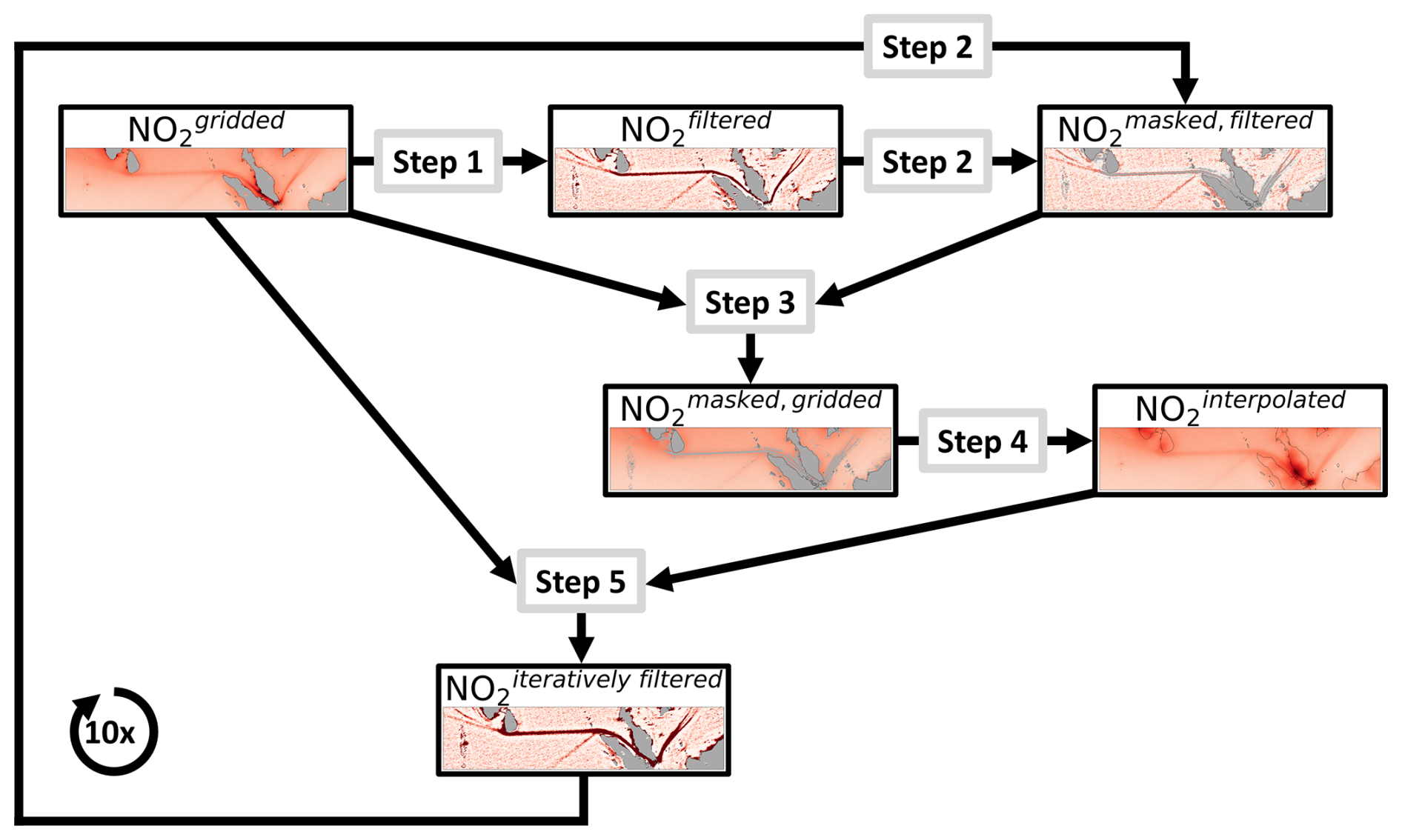
Figure 1 Schematic overview of the iterative high-pass filtering method applied to the gridded TROPOMI NO₂ tSCD. The outputs of the different procedure steps are depicted for a shipping lane in the Indian Ocean. After a thorough examination, an iteration number of 10 times proves to be the most efficient.

Several data selection criteria can be utilized to flag the filtered TROPOMI NO₂ data for specific meteorological and measurement geometry conditions to evaluate the impact of observational conditions on the analysis. This approach enables the analysis of which flagging variables impact the detection of the shipping signals and how they do so. The quality (qa) flagging includes only pixels with a quality value larger than 0.75, excluding measurements containing a cloud radiance fraction exceeding 50 %, having a large RMS, or exhibiting a very small AMF. The cloud fraction (CF) flagging considers only pixels with a cloud cover less than 0.5 to eliminate measurements affected by an extensive cloud cover. The cloud height (CH) flagging uses only pixels without clouds (clear-sky scenes) and with clouds at altitudes below 2 km (with no CF threshold) to avoid higher clouds that may shield the shipping NO₂ from the satellite view. The wind speed (wind) flagging retains only pixels with wind speeds between 0 and 5 m s⁻¹ to exclude conditions where the NO₂ is rapidly dispersed due to strong advection and related mixing. Lastly, the sun glint (sg) flagging identifies pixels defined as “sun glint is possible” (indicated by the TROPOMI variable “geolocation_flag = 2”), enabling the investigation of situations where the sensitivity for NO₂ near the sea surface is potentially increased due to the direct reflection of sunlight off ocean surface waves towards the satellite. The effects of these different data flagging criteria depend on the specific context in which they are applied. Thus, sun glint conditions can increase TROPOMI's sensitivity to detect NO₂ emissions from shipping, as previously demonstrated by Georgoulias et al. (2020) for individual ship plumes and by Riess et al. (2022). However, one issue in applying these flagging criteria is that the background noise increases due to the reduced number of available measurement values. Section 3.1 discusses the individual impacts of the various flagging criteria in detail, while no flagging criterion is applied to the tSCDs as a standard in this study.

Another essential aspect to consider is that the choice of the maps' color scale significantly affects the visualization of the shipping lanes. When a symmetric color range with equally distributed negative and positive limits is used, the negative values in some coastal regions become more prominent on the map (see Fig. B1). In contrast, shifting the values to a positive color range highlights the shipping lanes more effectively (see Fig. 2). This study focuses on the qualitative detection of shipping signals. Therefore, a positive color scale is used for the maps.

3 Global shipping signals in filtered TROPOMI NO₂ tSCDs

This section presents several regions where shipping signals in the filtered TROPOMI NO₂ data are detected using the introduced method. First, Fig. 2 shows a global map providing an overview of the detected NO₂ signals over the 6 years of analysis (from May 2018 to April 2024). As the standard criterion, no data flagging is applied to the filtered TROPOMI NO₂ tSCDs, as discussed later. A large number of shipping routes are directly visible on the global map, both the known shipping lanes, e.g., in the Mediterranean Sea, the Red Sea, and the Indian Ocean, and the previously undetected shipping lanes, e.g., in the Caribbean Sea to the Panama Canal, between Indonesia and Australia, and between Asia and North America. All regions where NO₂ signals from shipping are identified will be presented later in more detail. It is worth noting that all these shipping routes come directly from the TROPOMI NO₂ data without any tropospheric model a priori.

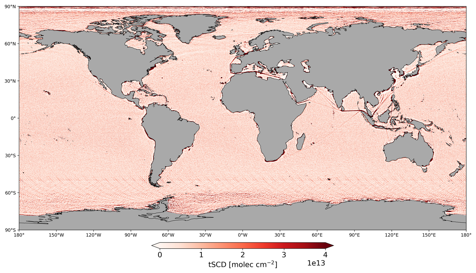
Figure 2 Overview of the NO₂ signals from 6 years of filtered TROPOMI data. Many shipping routes are identified, such as known ones, e.g., in the Mediterranean Sea, the Red Sea, and the Indian Ocean, and ones that have not been detected before in satellite data, e.g., towards the Panama Canal, between Indonesia and Australia, and between Asia and North America. A high-resolution, zoomed-in version of this global map is available at: https://www.iup.uni-bremen.de/doas/tropomi_ships.htm (last access: 28 August 2025). Figure B1 shows the corresponding global map of the filtered TROPOMI NO₂ tSCDs using a symmetric color scale to visualize also the negative values resulting from the high-pass filtering method, which occur mainly at coastlines around Europe and Asia.

Even though many shipping routes can be detected in the filtered TROPOMI NO₂ data, the global map overlaps with background noise. The noise results from using the high-pass filter, highlighting the very small NO₂ signals from ships but simultaneously amplifying the background noise. The stripe-like patterns oriented in the TROPOMI orbit direction are probably artifacts caused by the periodic overlapping of the S5P orbits. The Fourier filtering could not altogether remove them. In addition, the systematic artifacts around some land masses warrant careful consideration. These elevated NO₂ columns, particularly along coastlines and near islands, result from DOAS retrieval fit problems in inhomogeneous scenes where large intensity differences between adjacent measurements prevail, for example, along the sea ice edge or around permanently cloudy regions (Richter et al., 2020). This scene inhomogeneity effect is further amplified by the high-pass filtering, affecting the accuracy of the TROPOMI NO₂ measurements. This phenomenon and AMF effects are visible in the polar regions, where a distinct contrast appears between the typical background and a patterned distribution of NO₂ signals. Off the coast of Antarctica and the Arctic, these pronounced structures represent the average sea ice extent. The variation in NO₂ signals along the borders of ice and land surfaces is primarily caused by differences in the surface albedo, specifically, the fraction of sunlight reflected by a surface. Sea ice has a high albedo, reflecting a significant portion of sunlight, while the open ocean, with its lower albedo, absorbs most of the incoming light. This sharp contrast in reflectivity between the bright sea ice and the darker ocean surface results in a stronger NO₂ signal over sea ice, even when the actual NO₂ concentrations remain unchanged due to AMF effects. This AMF effect can also be observed over bright clouds, where the increased reflectivity also enhances the NO₂ signal in the measurements (Latsch et al., 2022). Applying the iterative filtering approach to the TROPOMI NO₂ data reduces the presence of these phenomena.

However, not all elevated NO₂ signals in polar regions are artifacts. For example, higher NO₂ signals are detected in the Bering Sea, which will be discussed later in Fig. 5, and in the Ross Sea near the Antarctic continent (Appendix Fig. B2a). As the CAMS-GLOB-SHIP data indicate (ECCAD, 2018; Granier et al., 2019), the elevated NO₂ signal in the Ross Sea can be assigned to shipping activities (Appendix Fig. B2b). The data reveal shipping routes to and from various research stations near the coast, including the Jang Bogo station, the Gondwana station, the Mario Zucchelli station, and the McMurdo station on Ross Island. The filtered NO₂ TROPOMI data were examined for the two polar seasons to ensure that the elevated signal may be attributed to shipping and not only to the research stations (not shown). In the Ross Sea, the higher NO₂ signal is detected only when the sea ice extent is minimal in summer (December to April), while during the winter season (June to November), the characteristic sea ice pattern dominates the TROPOMI NO₂ data in the polar region.

Figure 3 shows the seas surrounding the European continent, using different box sizes for both the longitude and latitude in the rolling mean applied to the high-pass filter. The choice of the box size defines the spatial size of NO₂ enhancements that are detected and, therefore, influences the characteristics and number of visible shipping routes. The primary route in the Mediterranean Sea, extending from the exit of the Suez Canal to the Strait of Gibraltar and continuing across the North Atlantic Ocean towards the English Channel, is consistently detected regardless of the box size. In contrast, more minor shipping routes, such as the direct shipping lane in the Black Sea leading into the Aegean Sea, encircling the Greek islands before reaching the Ionian Sea, and those in the Adriatic and Tyrrhenian seas around Italy, particularly between Sardinia and Corsica, are only faintly visible when using a smaller box size of approximately 0.25° (Fig. 3a). These routes grow increasingly pronounced with a larger box size of about 1° (Fig. 3b). Additionally, weaker signals in the North Sea and Baltic Sea are more visible with a 1° box size. However, the visualization of separated shipping lanes, such as the two one-directional shipping routes in the North Atlantic Ocean, which here are for the first time demonstrated in NO₂ satellite data, is possible only with a smaller box size (see also Sect. 3.1 for a detailed analysis of this lane separation). The NO₂ saturation near the coasts in the North Sea, around Italy, and the coasts of France, Spain, and North Africa, especially visible in Fig. 3b, is a result of the iterative high-pass filtering, which partially enhances the higher NO₂ signals near land with the same efficiency as the shipping lanes. Overall, a box size of 1° appears to be the most effective in highlighting the global shipping signals. Consequently, this study adopts a 1° box size as the standard, balancing detail with clarity to visualize shipping routes, especially on a global scale.

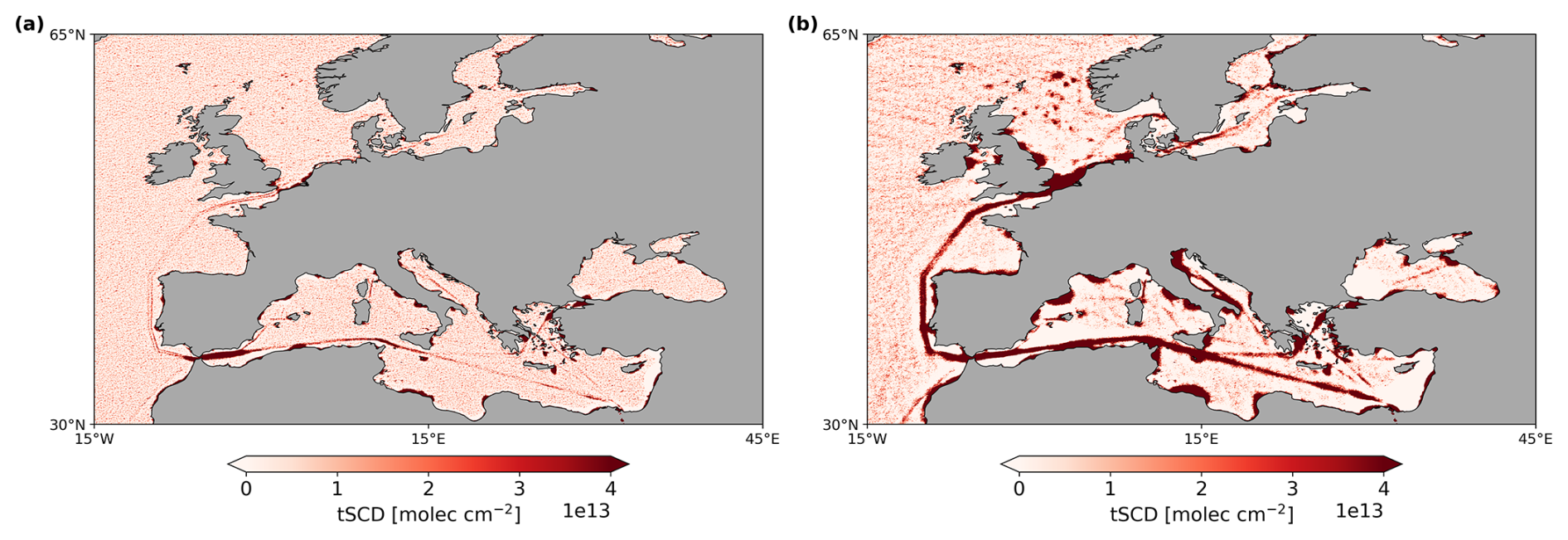
Figure 3 Filtered TROPOMI NO₂ signals from shipping activity in the European seas, analyzed with high-pass filters at different box sizes: approximately (a) 0.25° and (b) 1° in both longitude and latitude. The 0.25° box size reveals details of more minor shipping routes, such as the two shipping lanes in the North Atlantic Ocean, while weaker signals, such as in the Baltic Sea, and NO_x emissions from oil and gas platforms in the North Sea (see also Fig. 9) are more visible with the 1° box size. The NO₂ saturation near land, especially visible in the North Sea, around Italy, and at the coast of France, Spain, and North Africa in (b), is a result of the iterative high-pass filtering, which partially enhances the higher NO₂ signals at coastlines.

Nevertheless, another approach was tested, using two different box sizes depending on the distance from the coastline. This method of individual box sizes allows the implementation of the smaller box size of 0.25° for pixels close to the coastline, while the standard box size of 1° is used for all other pixels that are further away from the coastal pixels and in the open oceans. The advantages and disadvantages of this method are discussed below for a selected region, i.e., the seas around Europe, Africa, and Asia (see Fig. B3). Figure B3b shows the NO₂ signals of the different box sizes with a coastal area of 50 pixels (≈ 1.5°) from the shoreline, within which the smaller box size is used. In this case, the shipping lanes in narrow ocean regions such as the Persian Gulf are well resolved, the separated shipping routes in the Atlantic Ocean and the English Channel are visible, and the large NO₂ values near the coast caused by the scene inhomogeneity and high-pass filter effects are removed. However, the shipping lanes near land pixels that have the largest NO₂ values at a box size of 1°, such as the busy shipping route in the Indian Ocean from Sri Lanka to Indonesia and the shipping lanes in the Mediterranean Sea, are reduced or even canceled due to the smaller box size resolution, as in the Black Sea. Therefore, the effect of a smaller coastal region of only 17 pixels (≈ 0.5°) on the NO₂ signals is also investigated (Fig. B3c). Under this specification, the well-defined shipping lanes near the coast are displayed clearly and without interruptions. However, this coastal region is not wide enough to visualize the small-scale NO₂ signals in narrow regions such as the Persian Gulf. The main advantage of this approach is that the artifacts of high NO₂ values near the coast caused by the high-pass filtering are compensated for in most regions, regardless of the width of the coastal region. However, the effect of this method on the visualization of shipping lanes largely depends on the region and its proximity to the coast. In some areas, such as southeast of South Korea and Japan, inserting the values of the smaller box size close to the coast separates the artifacts from the land and thus could be perceived as shipping signals. The bottom line is that this method can significantly improve the detection of shipping signals and reduce background levels for specific regions, but its results are not consistent on a global scale. Therefore, the following analysis uses the standard box size of 1° to provide an overview of our method, which can be applied globally.

Previous studies have demonstrated that the prominent shipping lane in the Red Sea is detectable by various satellite instruments, including TROPOMI. Figure 4a shows high NO₂ values in this region, effectively highlighting the shipping lane as it enters the Arabian Sea. There, the route diverges in multiple directions, southward towards the Laccadive Sea and northward along the coast of Oman into the Gulf of Oman. No clear NO₂ signal is visible in the Persian Gulf because the limited spatial extent of the gulf and its proximity to the landmasses lower the ability to detect NO₂ emissions using the iterative high-pass filtering method with a 1° box size. Only the non-iteratively filtered NO₂ TROPOMI data with a smaller box size of 0.25° prove to be highly effective in visualizing the shipping route near the coast of Iran in this spatially limited region (see Appendix Fig. B4). Additionally, the NO_x emissions from offshore platforms are distinctly visible as isolated points in the middle of the Persian Gulf with the 0.25° box size. Furthermore, two separated shipping lanes in the Gulf of Aden, leading to and from the Red Sea, are also identified. However, it is important to note that the non-iteratively filtered NO₂ data with the 0.25° box size does not capture signals in the Arabian Sea as visibly as does the iteratively filtered NO₂ data with the 1° box size.

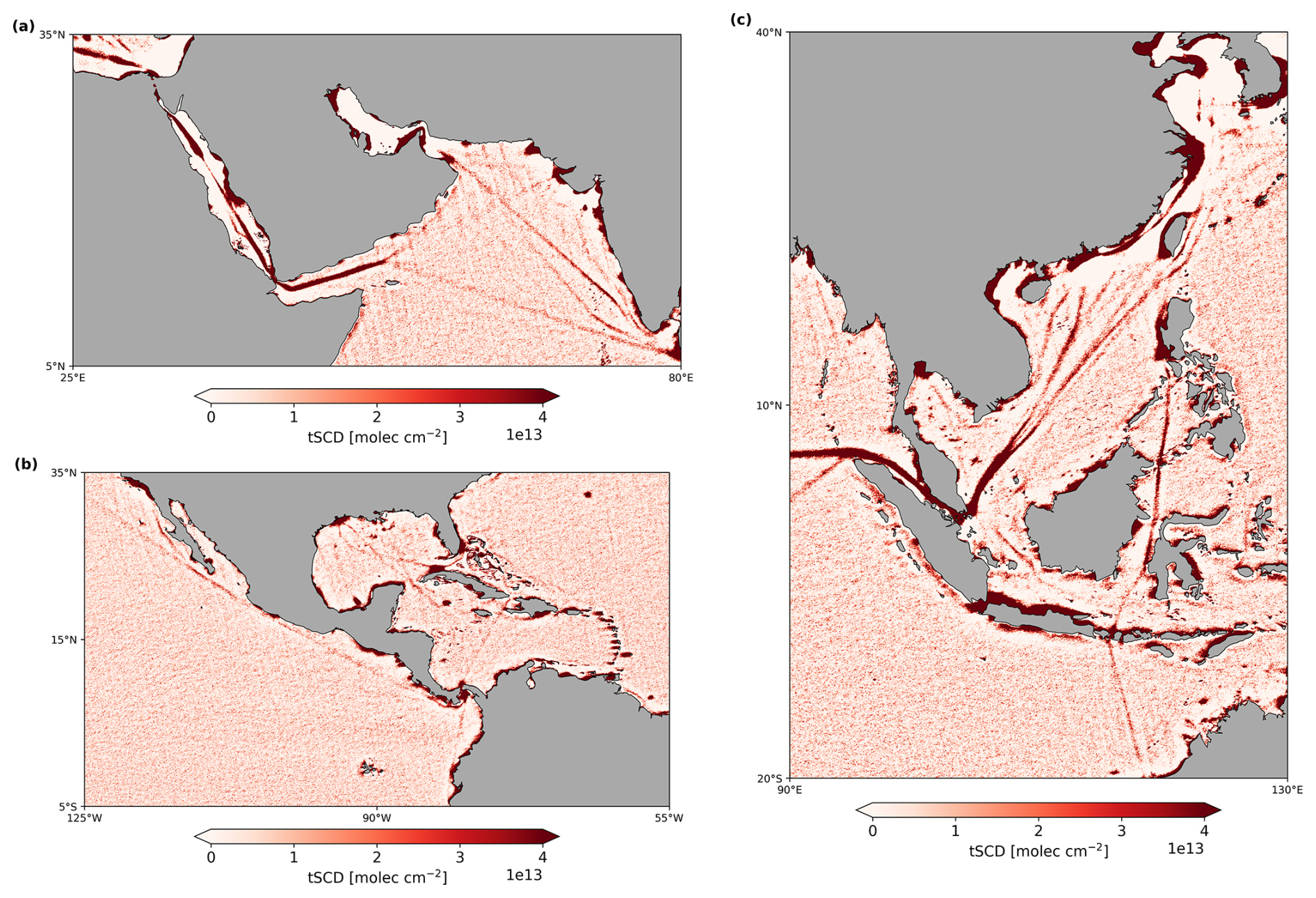
Figure 4 Filtered TROPOMI NO₂ signals from shipping activity in (a) the Red and Arabian seas, (b) the seas around Middle America, and (c) the South China Sea. NO_x emissions from offshore platforms are visible as elevated dot-shaped NO₂ values, e.g., in (a) the Persian Gulf, (b) the Gulf of Mexico, and (c) the Gulf of Thailand (see also Sect. 3.2).

Figure 4b presents a region where shipping signals have not been previously detected. In the Gulf of Mexico, two prominent shipping lanes originate near the port of Houston, intersecting again in the middle of the gulf. One of these routes extends as far as the North Atlantic Ocean near the Bahamas, while the other one continues into the Caribbean Sea. In this region, a distinct NO₂ signal traces a direct path from the strait between Cuba and Haiti to the Panama Canal, where the NO₂ concentrations are markedly elevated. Some outflow of NO₂ from the Caribbean Islands is also visible but probably not linked to shipping activities and enhanced at some coastlines due to the iterative high-pass filtering. However, NO_x emissions from offshore oil and gas platforms are identified in the Gulf of Mexico (see Sect. 3.2 for more details). In the Pacific Ocean, a single shipping signal is detected, stretching from the Panama Canal along the Mexican coast up to North America. Notably, higher NO₂ values are visible along the coast of the Baja California peninsula. Further south, a shipping route extends from the Panama Canal towards Ecuador and into the southern Pacific.

In Fig. 4c, a prominent shipping lane is visible in the Andaman Sea, where it is joined by a subtler route originating from South Africa (see Fig. 2), continuing through the Strait of Malacca towards Singapore. Farther northwest, this shipping lane divides into several distinct lines in the South China Sea, the first time these shipping routes have been identified in TROPOMI NO₂ data. Additionally, a clear NO₂ signal is detected along the coast of China, stretching from the South China Sea across the East China Sea and into the Yellow Sea. Two separated lanes are also visible in the Philippine Sea, just off the coast of Taiwan. Another clear shipping route extends directly from the Philippines, passing through the Makassar Strait and towards Australia. In the Gulf of Thailand, only a faint shipping signal is detected, which can be attributed to the 1° box size used in the high-pass filtering, as it is too coarse to capture fine details in this spatially limited region. However, elevated NO₂ values are visible as pronounced dots corresponding to NO_x emissions from offshore platforms. Along the southern coast of many islands, a region of enhanced NO₂ is found – on the one hand, another example of the artifact created by inhomogeneous scenes at some coastlines, and on the other hand, a result of the iterative filtering method.

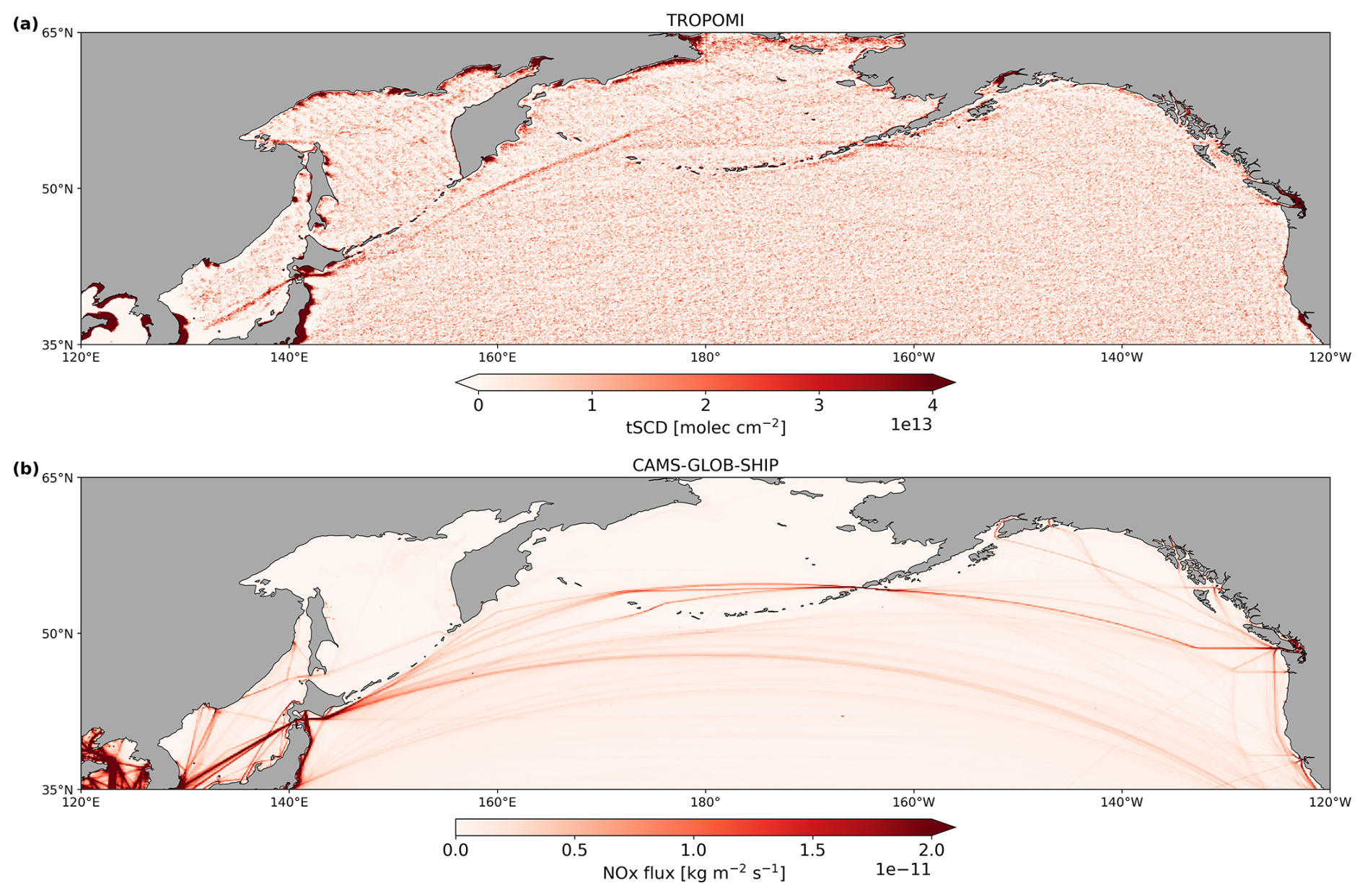
Figure 5 (a) Filtered TROPOMI and (b) CAMS-GLOB-SHIP NO₂ signals from shipping activity in the North Pacific correlate well for the two shipping routes between Asia and North America. The NO₂ signal in the Bering Sea is identified only in the filtered TROPOMI data and not tracked through the AIS-based CAMS-GLOB-SHIP data, possibly due to disabled trackers on board military or unauthorized fishing vessels. The CAMS-GLOB-SHIP data cover the years from 2018 to 2021 (ECCAD, 2018).

A distinct shipping route from the Korea Strait to the Tsugaru Strait in the Sea of Japan is detected in the filtered TROPOMI NO₂ data, as shown in Fig. 5a. Extending from the Tsugaru Strait, two shipping lanes are identified for the first time in satellite data in the North Pacific. The more southerly NO₂ signal, which connects to the shipping lane originating from the Panama Canal, is noticeably weaker than the northern lane, which diverges into two branches in the Bering Sea. One branch extends across the southern Bering Sea, reaching the Aleutian Islands (Alaska, USA) and continuing along the Salish Sea south of Vancouver Island (Canada). The other branch appears to go to the Alaskan mainland just north of Nunivak Island. This northern signal, previously undetected in satellite data and not typically associated with known shipping routes, indicates a need for comparison with the CAMS-GLOB-SHIP (Copernicus Atmospheric Monitoring Service for Global Shipping) data. CAMS-GLOB-SHIP is a global emission inventory based on AIS (Automatic Identification System) information and the Ship Traffic Emission Assessment Model (STEAM) to describe ship traffic activity. The CAMS-GLOB-SHIP inventory, version 3.2, provides global ship emissions on a 0.1° × 0.1° grid for the years 2018 to 2021, available from the ECCAD (Emissions of Atmospheric Compounds and Compilation of Ancillary Data) database (ECCAD, 2018; Granier et al., 2019). Notably, the CAMS-GLOB-SHIP data show no significant ship traffic activity in the northern Bering Sea, where this elevated NO₂ signal is detected in the TROPOMI data (Fig. 5b). This discrepancy suggests that ship activities in this region may not be fully captured in the CAMS-GLOB-SHIP inventory due to disabled AIS trackers, possibly linked to illegal or military operations. It is not uncommon for some ships, particularly military or unauthorized vessels, to turn off their AIS trackers, preventing the detection of their presence in certain areas, including in the CAMS-GLOB-SHIP data. Supporting this, the study by Welch et al. (2022) notes that the fraction of estimated total fishing vessel activity obscured by suspected AIS disabling events is highest in the northwest Pacific. This finding corresponds to the elevated NO₂ signal detected in the TROPOMI data for this region in the absence of AIS signals despite sufficient satellite reception quality. Therefore, this research supports the hypothesis that the signal is real but cannot be tracked through AIS data due to disabled trackers.

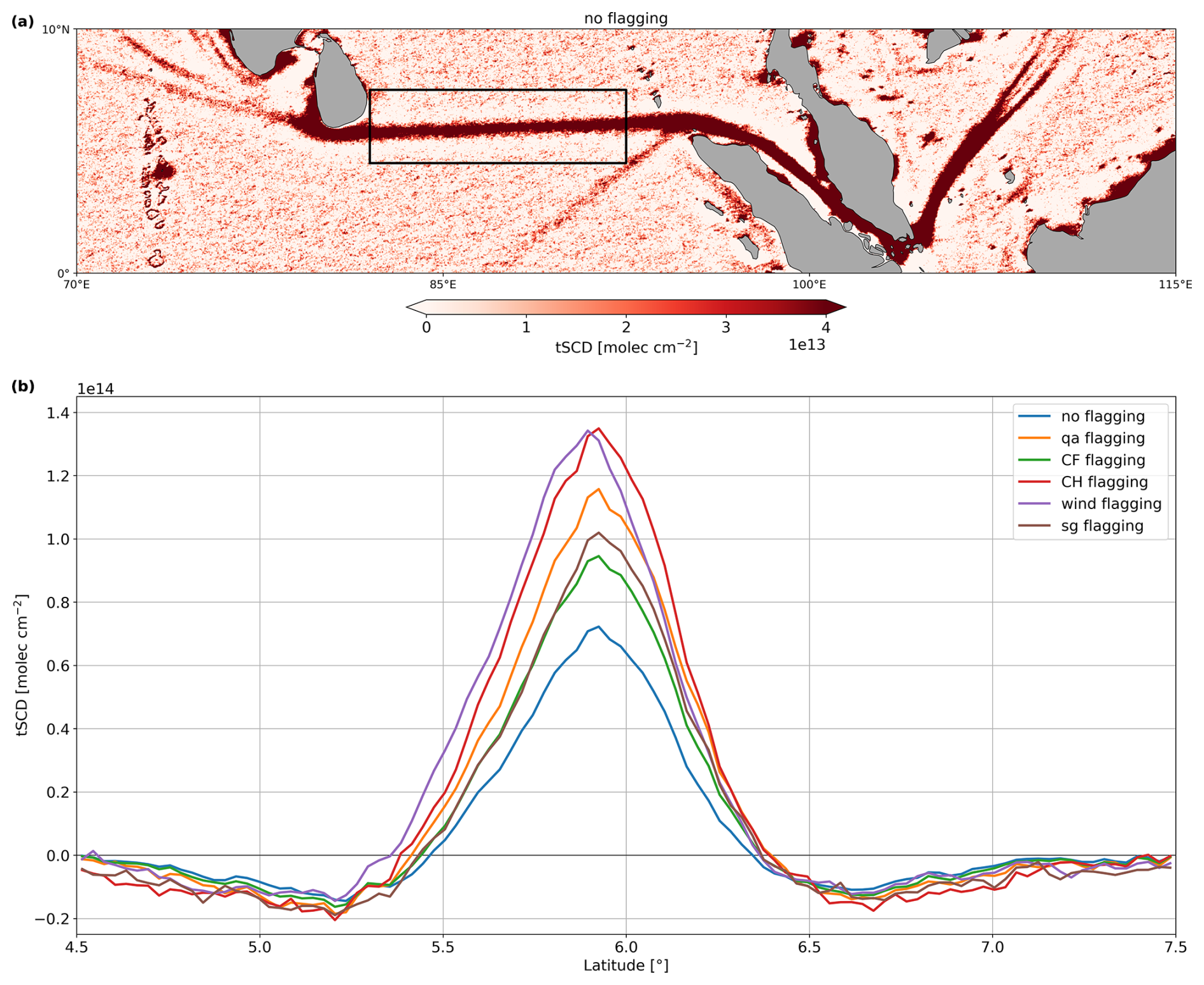
Figure 6 (a) Filtered TROPOMI NO₂ signals from shipping activity in the Indian Ocean, between Sri Lanka, Indonesia, Malaysia, and Singapore, without data flagging. The black rectangle highlights the area shown in (b), which displays the cross-sections of the shipping lane for the different flagging criteria: all pixels included (blue) and only pixels including qa >0.75 (orange), CF <0.5 (green), CH <2 km (red), 0 m s⁻¹ < wind speed $<\mathrm{5}\mathrm{m}{\mathrm{s}}^{-\mathrm{1}}$ (purple), and sg possible situations (brown). The curves represent the longitudinal average from 82 to 92.5° E as a function of latitude.

3.1 Shipping lane cross-sections

The distinct shipping route from Sri Lanka to the Strait of Malacca, located between Malaysia and Indonesia, has already been discussed in other publications and is also clearly visible in the filtered TROPOMI NO₂ data (Fig. 6a). Here, we focus on the cross-section of this shipping lane, marked by the black rectangle in Fig. 6a, to investigate the individual impacts of various flagging criteria (see Sect. 2) on the NO₂ signal distribution along the shipping lane. Figure 6b displays the longitudinal average of the NO₂ tSCD from 82 to 92.5° E, plotted as a function of latitude from 4.5 to 7.5° N for the different flagging criteria. All curves show a prominent peak at approximately 5.9° N and two minima at around 5.2 and 6.7° N. It should be mentioned that the NO₂ distribution heights and widths depend on the number of iterations of the high-pass filtering procedure: the more iterations, the higher and broader the peaks, as less diluted NO₂ from ships is included in the smoothed background map. As expected, the NO₂ column peak is lowest, and the background values are highest when no flagging is applied, resulting in the lowest variability among the curves. Applying flagging criteria leads to higher NO₂ peaks with differences of at least 2 × 10¹³ molec. cm⁻² for the curve flagged for cloud fraction (CF) and up to 6 × 10¹³ molec. cm⁻² for the curves flagged for cloud height (CH) and wind. By comparison, the differences at the minima or more general for the background values are lower, not exceeding 1 × 10¹³ molec. cm⁻². The negative values are attributed to the high-pass filter, which emphasizes the larger shipping signal values while causing the background values directly adjacent to the shipping lanes to appear negative due to the rolling mean applied in this method (see also Fig. B1). The six curves show less variation as the distance from the peak of the shipping route increases, where the rolling mean has less influence than around the highest values. Using the iterative filtering method, the values around the shipping lanes are not as negative as when applying the high-pass filter only once.

Regarding the NO₂ signal peak, flagging for small CFs and sun glint (sg) has the lowest effect on the NO₂ signal distribution, aside from no flagging. When quality (qa) flagging is applied, the NO₂ peak increases slightly, although not as much as with the CH and wind flagging criteria. The latter is notably shifted for low wind speeds. This shift may be attributed to a correlation between wind speed and direction. Beirle et al. (2004) identified a strong seasonal asymmetry in the NO₂ signal peak due to the impact of the Intertropical Convergence Zone (ITCZ) on the ship track in this region. In calm wind conditions, the NO₂ emissions from ships may accumulate and form a more concentrated plume at a specific location. Conversely, in higher wind conditions, captured by the other flagging criteria, the NO₂ from ships disperses more quickly, leading to a more spread-out signal. Therefore, the peak for low wind speeds may be shifted towards the location of the shipping lane where the NO₂ accumulates. Flagging for the lowest CHs is among the most effective criteria due to the increased NO₂ peak. In addition to the fact that this flagging criterion includes the clear-sky scenes, one potential reason for this higher peak is that low clouds can reflect more sunlight towards the satellite, enhancing the sensitivity of the TROPOMI instrument for NO₂ above the clouds. This increased sensitivity may lead to higher slant columns of NO₂ in the shipping lanes when only the lowest CHs and clear-sky scenes are considered. It should be noted that the flagging criteria have different effects on the detected NO₂. For example, wind flagging selects situations where there is actually more NO₂ in the atmosphere, while the other flagging criteria select situations that improve the visibility of NO₂. The latter can, at least in principle, be compensated for by a suitable AMF, while the higher NO₂ values at low wind speeds are real and should also appear in the tVCDs, as shown by Riess et al. (2022).

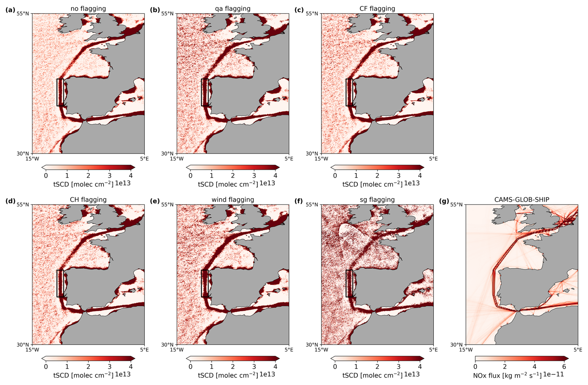
Figure 7 (a–f) Filtered TROPOMI and (g) CAMS-GLOB-SHIP NO₂ signals from shipping activity in the Atlantic Ocean near the coast of Portugal; filtered TROPOMI data with (a) no flagging, (b) qa flagging, (c) CF flagging, (d) CH flagging, (e) wind flagging, and (f) sg flagging. The rectangles highlight the area of the cross-sections shown in Fig. 8. The two separated shipping lanes visible in the filtered TROPOMI NO₂ data correlate well with the CAMS-GLOB-SHIP data, covering the years from 2018 to 2021 (ECCAD, 2018).

Overall, the choice of flagging criteria significantly impacts the observed NO₂ signal along the shipping lanes. Based on the results discussed above, one would therefore apply qa flagging and possibly also flagging for low clouds to improve the detection of weak shipping signals. However, applying these criteria has challenges, primarily due to the reduced number of available measurements. This reduction leads to a deterioration in the signal-to-noise ratio, as shown in Fig. 7a–f, which presents the shipping lane in the eastern North Atlantic region under different flagging conditions. The background noise is low when no flagging is applied (Fig. 7a). In contrast, the background noise significantly increases with the application of the flagging criteria (Fig. 7b–f), particularly sg flagging (Fig. 7f), due to the strongly reduced number of measurements. Furthermore, a pronounced artifact emerges south of Great Britain, mirroring the shape of the sg flagging area in the TROPOMI data but bearing no relation to any actual shipping signals.

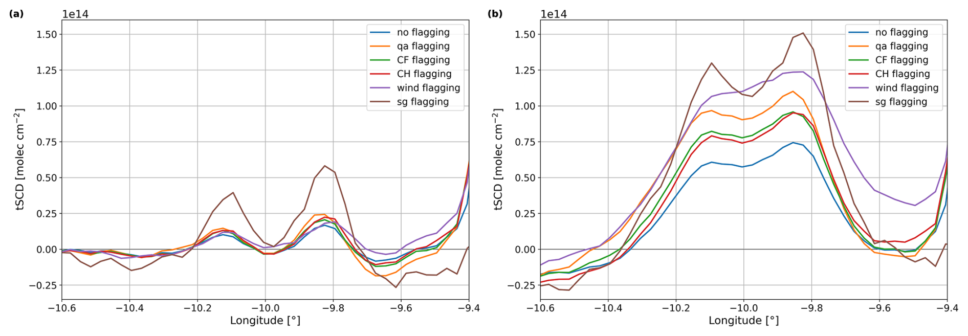
Figure 8 Cross-sections of the filtered TROPOMI NO₂ shipping lanes in the Atlantic Ocean near the coast of Portugal (rectangles in Fig. 7) for the different flagging criteria using different box sizes of approximately (a) 0.25° and (b) 1° in both longitude and latitude for the high-pass filter (corresponds to Fig. 3). The curves represent the latitudinal average from 38.5 to 43.3° N as a function of longitude. The elevated NO₂ values at larger longitude (−9.4°) reflect that the NO₂ signal increases near land masses – here Portugal – resulting from the iterative high-pass filtering.

Examining the shipping lane in the Atlantic Ocean near the coast of Portugal, marked by the black rectangle in Figs. 7a–f, Fig. 8 displays the latitudinal average of the NO₂ tSCD from 38.5 to 43.3° N, plotted as a function of longitude from 10.6 to 9.4° W for the different flagging criteria using high-pass-filter box sizes of 0.25 and 1°. Using a smaller box size of 0.25° in the high-pass filter (Fig. 8a) reveals a double-peaked pattern in the NO₂ signal for all flagging criteria, with the effect under the sg flagging particularly pronounced and its peaks being larger than about 2.5 × 10¹³ molec. cm⁻² compared to the peaks of the other curves. With a 1° box size (Fig. 8b), the NO₂ values of the two peaks are generally around 5 × 10¹³ molec. cm⁻² for the no flagging case and even 9 × 10¹³ molec. cm⁻² for the sg flagging, higher than those observed with a 0.25° box size. However, the two peaks are less pronounced, except for the ones with sg flagging, which again show a distinct double-peak pattern and elevated NO₂ column levels, differing from the other peaks by approximately 2.5 × 10¹³ molec. cm⁻² compared to the peaks with no flagging and up to 7.5 × 10¹³ molec. cm⁻² compared to the wind-flagged peaks. This finding corresponds to the observations in Fig. 3, where the northeast Atlantic shipping lane is clearly separated with the smaller box size (Fig. 3a), whereas the NO₂ signal itself is much stronger with the 1° box size (Fig. 3b). The two peaks observed are attributed to ships moving in opposite directions along the primary shipping route off the coast of Portugal, where the respective travel directions are clustered. This observation is supported by the CAMS-GLOB-SHIP emission inventory (ECCAD, 2018; Granier et al., 2019), which indicates two distinct lines within the main route (Fig. 7g).

Both the 0.25° and the 1° box sizes show elevated NO₂ values at −9.4° longitude (Fig. 8a and b), reaching similar values of around 0 to 5 × 10¹³ molec. cm⁻². These elevated NO₂ values result from the closeness to the Portuguese coast, where the NO₂ signal increases probably due to land-based sources and is enhanced due to the high-pass filtering effect in areas near the shipping lane, like the negative NO₂ values, e.g., at −10.6° longitude. Notably, again, the curve with wind flagging shows, apart from the sg flagging curve, the largest NO₂ values and is slightly shifted. This result supports the expectation that low wind conditions would lead to NO₂ accumulation and amplify the signal. However, a less pronounced double-peak structure is found, especially for the 1° box size (Fig. 8b). A small gap in the southern part of the shipping signal in the cross-sectional area (Fig. 7e) suggests that the reduced number of measurements due to the flagging may contribute to this effect. This signal narrowing can smear the two-peak pattern, especially when using the 1° box size, where the influence of the high-pass filter is more substantial. Comparing the results of this region to the Indian Ocean cross-sections, the curve with CH flagging shows smaller NO₂ values than with the other criteria. It is more similar to that flagged for CF. As low cloud conditions are prevalent in the North Atlantic, the clear-sky scenes do not dominate the curve with CH flagging. Hence, this lower peak can be explained by the fact that the NO₂ in this region is predominantly below the clouds, unlike in the Indian Ocean, where some of the NO₂ is presumably present above the clouds. As a result, the clouds shield the NO₂ in the Atlantic Ocean, resulting in smaller NO₂ slant columns. The pronounced effect of sg flagging on the NO₂ signal can be attributed to the increased sensitivity of TROPOMI to NO₂ absorption near the sea surface due to the enhanced reflectivity of sunlight on the water. This also explains the more distinct double-peak pattern, as the ship plumes are better separated near the surface, where sun glint has the most substantial effect. At higher altitudes, the plumes tend to mix, reducing their distinctiveness. While this effect amplifies the NO₂ signal, this enhancement does not significantly improve the shipping lane detection due to increased background noise. Therefore, non-flagged data are preferred for detecting NO₂ emissions from global shipping lanes in this study.

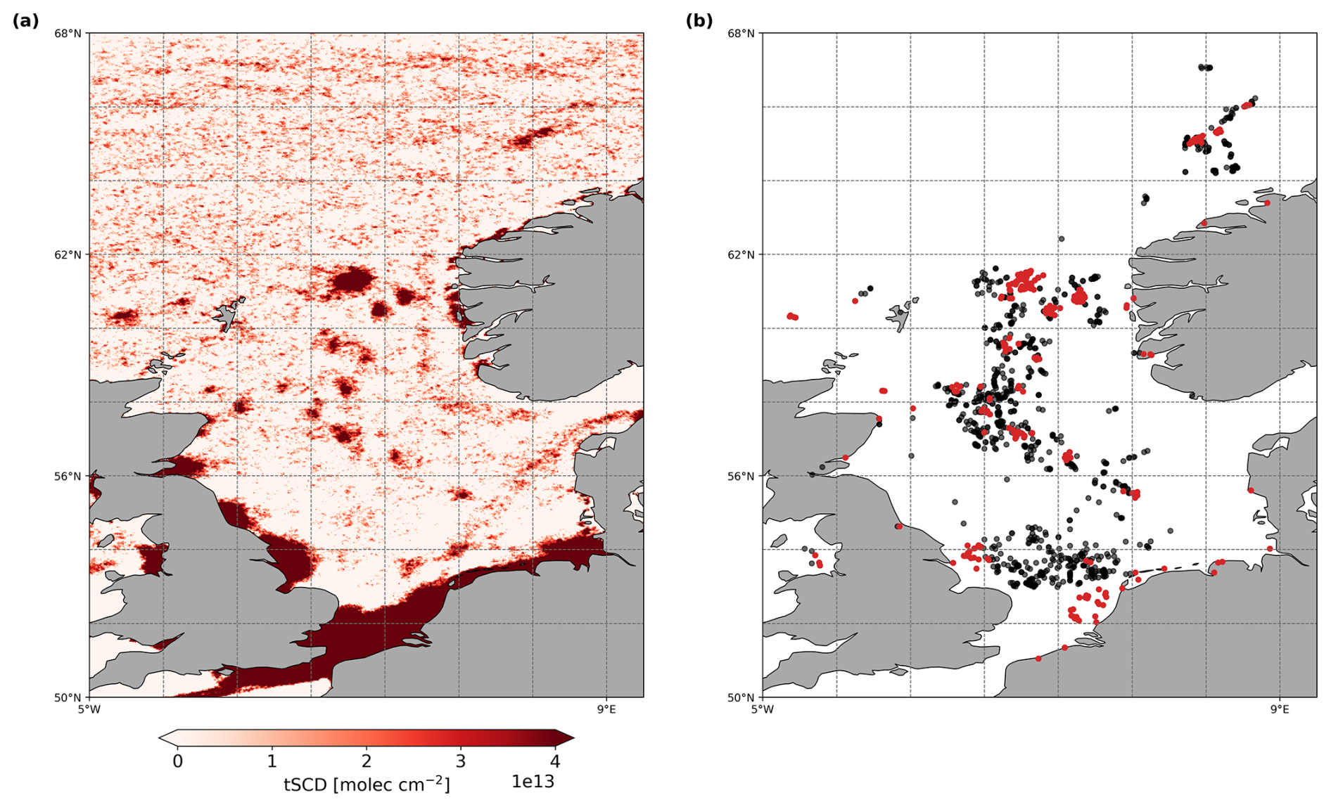
Figure 9 (a) Filtered TROPOMI NO₂ signals in the North Sea, and (b) locations of oil and gas platforms (dots). The hotspot regions where the NO₂ signals exceed 3.5 × 10¹³ molec. cm⁻² (a) correlate well with the locations of offshore installations, and those are indicated by the red dots (b). In other regions where oil and gas platforms are located, the NO₂ values show no significant enhancement, possibly due to variations in the emission rates and the high-pass filtering effect. The offshore installations are classified as “operational” in the OSPAR emission inventories for 2019 and 2021 (ODIMS, 2021).

3.2 Offshore platform detection

The method presented in this study enables the detection of NO₂ emissions not only from shipping activities but also from offshore oil and gas platforms, which release NO_x during drilling and gas flaring. Figure 9a highlights NO₂ hotspots in the North Sea, particularly in the northern region. These areas of elevated NO₂ concentrations correspond to clusters of offshore oil and gas installations documented in the OSPAR (Oslo and Paris Commission) inventory (ODIMS, 2021). The dots in Fig. 9b indicate the positions of offshore oil and gas platforms listed as operational in the OSPAR inventory for 2019 and 2021. Many of these platform locations match closely with NO₂ hotspots in the filtered TROPOMI NO₂ data; those exceeding 3.5 × 10¹³ molec. cm⁻² in Fig. 9a are indicated with red dots in Fig. 9b. Some larger NO₂ hotspot areas, such as the western section of the North Sea and north of Great Britain, overlap with only a few single offshore installations in the OSPAR data. One reason for being visible in the filtered TROPOMI NO₂ data might be that these platforms emit high levels of NO_x due to their size or operational intensity, particularly those involved in extensive flaring or high production. Additionally, local meteorological conditions, including wind direction and temperature inversions, can trap NO₂ or slow its dispersion, resulting in concentrated signals from just a few sources. Furthermore, the OSPAR inventory provides a snapshot of various platform statuses, including operational, decommissioned, closed down, unknown, derogation, dismantled, and under construction. Consequently, there may be gaps or delays in the OSPAR inventory regarding smaller or less permanent installations, leading to discrepancies between the detected hotspots and the documented platform locations.

Notably, the shipping lane from the Skagerrak Strait northward along the Norwegian coast is identified, with NO₂ signals further intensified where this lane intersects oil and gas platform sites due to an accumulation from both the ship and platform emissions. However, in the southern North Sea, the clusters of oil and gas installations show little to no correlation with increased NO₂ concentrations. This discrepancy may result from significant variations in the emission rates from individual platforms; older or less active platforms may emit lower levels of NO₂, leading to less pronounced signals despite their presence. Additionally, atmospheric conditions should be considered, such as prevailing winds and temperature patterns, or geographical features, including ocean currents, island formations, and proximity to land masses. These factors can significantly affect how NO₂ emissions are dispersed or concentrated. In some areas, wind patterns may carry NO₂ molecules away from their sources, reducing the concentration near the sources and causing a mismatch between high NO₂ concentrations and the platform locations. Furthermore, interference from other NO₂ sources, such as coastal cities on the eastern coast of Great Britain, possibly from wind-blown urban traffic and rural sources, may contribute to the background NO₂. The shipping lane from the English Channel towards the Skagerrak Strait is overshadowed by a NO₂ saturation, effectively diluting the apparent impact of emissions from nearby platforms and ship lanes. These elevated NO₂ values result from the high-pass filtering effect near land. Finally, detection limitations may also play a significant role. Platforms with lower emissions or those spread over a larger area might fall below the detection threshold of TROPOMI, making their NO₂ contributions less visible.

Figure 10 Same as Fig. 9 but in the Gulf of Mexico. The oil and gas platforms are listed as NO_x sources in the BOEM 2021 emission inventory (BOEM, 2021).

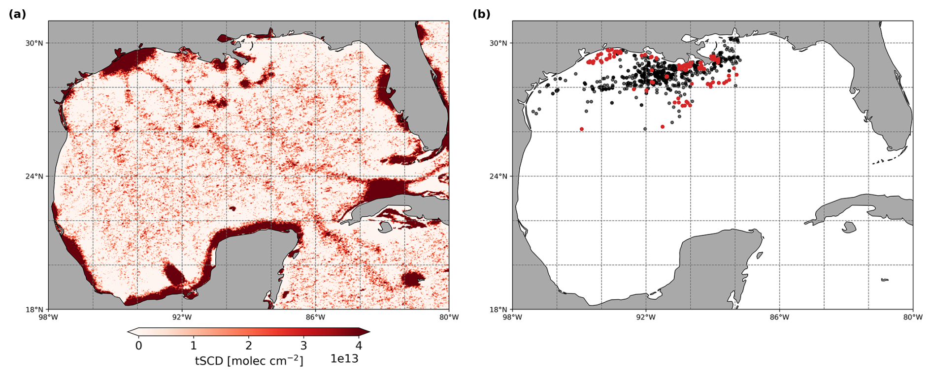
The same phenomenon is observed in the Gulf of Mexico (Fig. 10), where numerous oil and gas platforms are situated near the US coast. Location data for these offshore installations (Fig. 10b) were obtained from the Outer Continental Shelf (OCS) Emissions Inventory, provided by the Bureau of Ocean Energy Management (BOEM) for the year 2021 (Thé et al., 2022). Not all clusters of these installations are visible in the filtered TROPOMI NO₂ data (Fig. 10a), potentially due to factors discussed previously, such as platform size, distance from the shore, and emission levels. At some coasts, especially where the shipping lanes from Houston enter the gulf, the high-pass filtering amplifies the NO₂ values, leading to circumstantial agreement of high NO₂ and platform locations. However, some installations, particularly those farther offshore, unaffected by the high-pass filtering artifacts, align prominently with NO₂ hotspots detected in the filtered TROPOMI NO₂ data. This observation supports findings from Fedkin et al. (2024), who investigated NO₂ trends from offshore oil and gas operations in the Gulf of Mexico. Their study includes a comparable regional map that displays NO_x emission hotspots from the BOEM data, which correlate well with the areas of elevated NO₂ values shown in Fig. 10a.

It should be noted that the elevated NO₂ signals detected in the southern Gulf of Mexico, particularly around the Bay of Campeche near the Mexican coast, as well as in the Caribbean Sea, are likely due to sandbanks or small, unregistered islands rather than oil and gas platform emissions. These signals result from the inhomogeneity effect in the TROPOMI measurements, where variability in surface reflectance amplifies the NO₂ signal even in the absence of emission sources. However, these results suggest that the TROPOMI data can effectively identify offshore oil and gas installations with significant NO₂ emissions, underscoring their value as a tool for monitoring environmental impacts from offshore operations.

4 Comparison between the filtered TROPOMI NO₂ tVCDs and the CAMS model

This study focuses on a qualitative detection of shipping NO₂ in TROPOMI tSCDs. However, it is of value to compare the retrieved tropospheric NO₂ vertical columns (tVCDs) with those from atmospheric models. For this, the NO₂ tVCDs from the Copernicus Atmosphere Monitoring Service (CAMS, Peuch et al., 2022) are used. CAMS data for which a TROPOMI measurement was present are used, matching both overpass time and cloud filtering. The resulting dataset has a spatial resolution of 0.4° × 0.4° and covers 5 years (2019–2023). To ensure a consistent analysis, the CAMS model data are high-pass filtered with the same settings as the TROPOMI data, including a 10-fold iteration. Consequently, 3 pixels of the CAMS model data are used for the rolling mean applied to the high-pass filter to maintain the 1° box size. The filtered TROPOMI NO₂ tSCDs are converted into tVCDs to compare the modeled CAMS data and the TROPOMI measurement. This conversion is performed by dividing the tSCDs by a constant AMF of 0.8. This method is not as precise as using pixel-specific AMF values because the AMF is affected by many factors, as discussed in Sect. 2. However, this approach provides a sufficient approximation for a simplified comparison to assess whether the shape and magnitude of the NO₂ distributions along selected shipping lanes differ between the modeled and observed datasets.

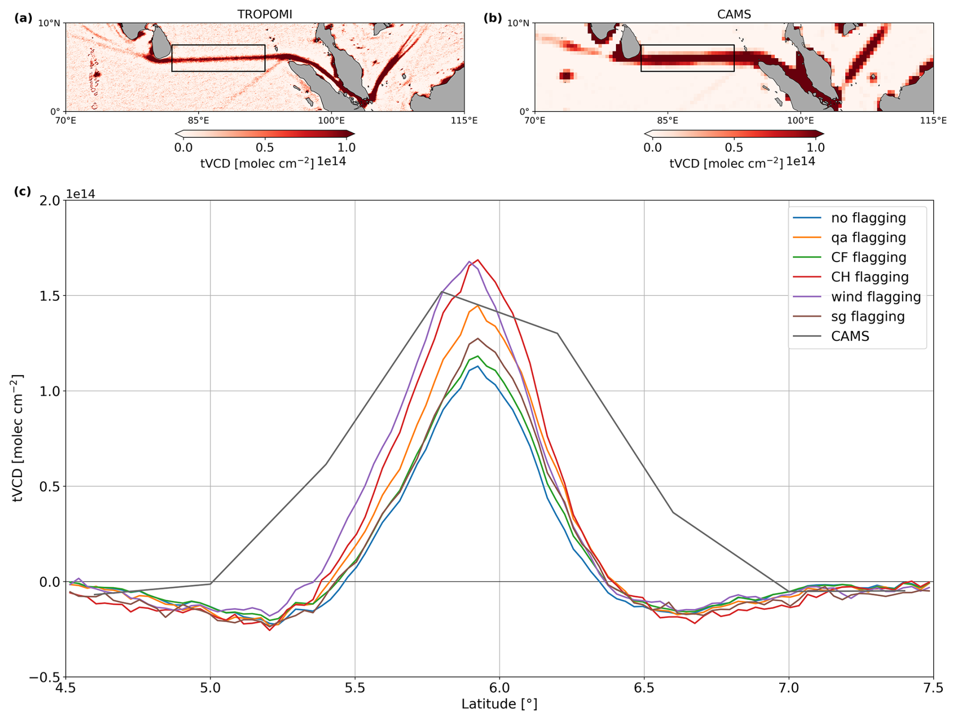
Figure 11 Same as Fig. 6 but with (a) the filtered TROPOMI NO₂ tVCDs with no flagging, (b) the high-pass-filtered CAMS NO₂ tVCDs, and (c) the cross-sections of the shipping lane for the different TROPOMI flagging criteria and the CAMS model data. The curves of the two datasets show a similar distribution peak, but the area under the high-pass-filtered CAMS tVCD curve is more extensive than under those of the filtered TROPOMI tVCDs. This broader FWHM in latitude of the CAMS curve is due to the coarser resolution of the CAMS model data, which are retrieved on a 0.4° × 0.4° grid for the years from 2019 to 2023 with cloud flagging.

Figure C1b highlights prominent global shipping lanes in the high-pass-filtered CAMS data. However, the NO₂ saturation near land masses of the CAMS model data complicates the identification of shipping emissions in some regions (not shown). For example, in areas such as the Mediterranean Sea, shipping-related NO₂ emissions are not as distinct in the high-pass-filtered CAMS data compared to the filtered TROPOMI NO₂ data (Fig. C1a) due to the dominance of land emissions. This disparity is partially attributed to the coarser spatial resolution of the CAMS model (0.4° × 0.4°) compared to the finer grid of the filtered TROPOMI NO₂ data (0.03° × 0.03°). The resolution difference becomes more noticeable when examining small-scale shipping lanes such as those in the Indian Ocean. Individual pixels are conspicuous in the high-pass-filtered CAMS NO₂ tVCDs (Fig. 11b), whereas the filtered TROPOMI NO₂ tVCDs (Fig. 11a) provide more detailed spatial patterns. Despite this, both datasets detect the position of the shipping lane, as demonstrated in the cross-sections, where the peak orientations of the distributions are comparable (Fig. 11c). In the CAMS NO₂ tVCD retrieval, the cloud flagging considers only cloud cover. This flagging criterion is most likely comparable to the qa flagging used in the filtered TROPOMI NO₂ data. The similar peak heights of the CAMS curve and the qa-flagged TROPOMI curve with approximately 1.5 × 10¹⁴ molec. cm⁻² confirm this assumption. However, the CAMS peak has a broader full width at half maximum (FWHM) in latitude than the sharper peaks in the TROPOMI data. Additionally, the background values of the high-pass-filtered CAMS NO₂ tVCDs are generally constant, in contrast to the highly varying TROPOMI tVCDs. Both differences of the two datasets are attributed to the coarser spatial resolution of the CAMS model data.

Additional analysis of the shipping lanes near Portugal in the North Atlantic Ocean and off the coast of West Africa in the South Atlantic Ocean is provided in Appendix C (Figs. C2 and C3, respectively). While the spatial positions of the NO₂ signals from shipping correlate well between the modeled and measured data for the shipping lanes near Portugal (Fig. C2c), the magnitude of the high-pass-filtered CAMS NO₂ tVCDs is significantly higher, exceeding the filtered TROPOMI NO₂ tVCDs by at least a factor of 2 to 3, depending on the different TROPOMI flagging criteria. Possible reasons for the large differences between the TROPOMI and CAMS NO₂ tVCDs are that in the CAMS model, the NO_x emissions from shipping are overestimated, or the chemistry in and the dilution of the ship plumes are inadequate. The latter means that, on the one hand, the photochemistry and the homogeneous and heterogeneous chemistry of NO_x in the CAMS model at the latitude and longitude grid of 0.4° × 0.4° do not remove enough NO_x. On the other hand, the high NO₂ concentrations from shipping are diluted over the size of the coarse-scale model grid cell in the CAMS model. However, in reality, the NO₂ is confined to narrow plumes. This instant dilution approach in CAMS could lead to overestimated NO_x concentrations from shipping over the oceans, as shown by Vinken et al. (2011).

For the shipping route in the South Atlantic (Fig. C3c), the peak of the CAMS curve is twice as large as those of the TROPOMI curves, which do not exceed 0.5 × 10¹³ molec. cm⁻². It appears to be slightly shifted due to the lower number of values resulting from the coarser spatial resolution. The difference between the two datasets is small with these standard settings. However, Fig. C4 shows that the high-pass-filtered CAMS NO₂ data for this shipping lane strongly depends on the masking threshold used in Step 2 of the high-pass filtering method (see Sect. 2). When the masking threshold value is lowered to ±1 × 10¹³ molec. cm⁻², the high-pass-filtered CAMS NO₂ tVCDs increase extraordinarily and are at least 4 times higher than with the standard threshold of ±3 × 10¹³ molec. cm⁻² (Fig. C3). The higher peak is accompanied by a much broader FWHM, so the shipping lane expands over the entire polygon area. This large dependence on the choice of masking threshold is found only for the shipping lane in the South Atlantic and only for the CAMS NO₂ data when considering the three selected regions. In contrast, the TROPOMI data show slightly higher peaks, where the difference is consistent and comparable to the other shipping lanes. Therefore, it should be kept in mind that applying the high-pass filter to the CAMS model data may result in large changes in the values in some regions, depending on the threshold value chosen.

5 Summary and conclusions

This study demonstrates the potential for qualitatively detecting NO₂ signals from global shipping routes using filtered S5P TROPOMI NO₂ data. By focusing on NO₂ tSCD rather than tVCD, a more objective identification of NO_x emissions from shipping is obtained, benefiting from the enhanced spatial resolution and avoiding artificial ship tracks introduced by the a priori profiles, associated with limitations of the AMFs derived from the coarse TM5 model, which only inadequately captures localized emissions. The preprocessing methods, such as smoothing of the stratospheric field and iterative high-pass and Fourier filtering, significantly improve the detection of global shipping lanes in the TROPOMI NO₂ data and enable shipping lanes previously undetectable in satellite observations or obscured in AIS-tracked data to be identified.

The influence of the box size in the high-pass filter on interpreting the TROPOMI NO₂ data is examined. Smaller box sizes enhance the visibility of narrow features like the separated shipping lanes in the North Atlantic or several more minor shipping routes in the Mediterranean Sea. In contrast, larger box sizes produce overall stronger NO₂ signals. This study identifies a 1° box size as appropriate for balancing NO₂ signal detection with minimized background distortion, but other choices may be more appropriate for local studies. The high-pass filtering also emphasizes inhomogeneity effects on NO₂ signals, especially in regions with varied surface reflectance near coastlines, sea ice, and islands. These surface inhomogeneities result in artificially elevated NO₂ values, as contrasting surface types affect reflectivity. Coastal and polar regions, in particular, exhibit these artifacts, complicating accurate emission source identification.

Several prominent TROPOMI NO₂ signals attributable to major shipping lanes, such as in the Red and Arabian seas, the Gulf of Mexico, and the seas of Asia, are successfully detected in the filtered TROPOMI data. Many additional identified shipping routes have never been shown in satellite NO₂ data before. The high-resolution images can be browsed at https://www.iup.uni-bremen.de/doas/tropomi_ships.htm (last access: 28 August 2025). The NO₂ signals reveal a strong correlation with shipping activities, as confirmed by the CAMS-GLOB-SHIP inventory (ECCAD, 2018; Granier et al., 2019). For the first time, the two separated shipping lanes near the coast of Portugal and towards the British Channel could be identified in satellite NO₂ data. This study also detected unknown shipping routes, for example, in the Bering Sea, where AIS data may be incomplete due to disabled trackers, highlighting the limitations of traditional AIS monitoring in capturing all shipping activities, particularly for military and unauthorized vessels operating in sensitive regions.

Moreover, this study analyzes the impact of flagging criteria, such as quality value, cloud fraction, cloud height, wind speed, and sun glint, on the NO₂ signal distribution along shipping lanes in the Indian Ocean and off the coast of Portugal. The cross-sections of the shipping route from Sri Lanka to the Malacca Strait reveal a pronounced NO₂ peak, with signal intensity varying depending on the applied flagging criteria. Non-flagged data produce the lowest NO₂ peak, while flagging generally increases the peak intensity at the lane's center. The strongest signals occur under low cloud heights, attributed to increased reflectivity and TROPOMI's enhanced sensitivity to NO₂ near the surface. Low wind speeds also influence the signal, causing an increase and slight shift in the peak location, likely due to NO₂ accumulation in calm conditions. These findings underscore the importance of selecting appropriate flagging criteria when using satellite data to monitor NO_x emissions, as each criterion can significantly influence the signal strength and the number of available measurements. In the shipping route off the coast of Portugal, a consistent double-peak NO₂ pattern is observed across all flagging criteria, particularly when using a smaller box size of 0.25° in the high-pass filter. This pattern corresponds to the structure of ships traveling in two directions along the main route, as confirmed by the CAMS-GLOB-SHIP inventory. Although a larger box size of 1° reduces the visibility of the double-peak pattern, it amplifies the overall NO₂ signal for all flagging criteria. The application of sun glint flagging further enhances the NO₂ signal due to increased surface reflectivity. However, this also diminishes overall lane detection effectiveness by increasing background noise from reduced measurement availability. Consequently, non-flagged data are preferred for presenting global NO₂ emissions from shipping, as they provide the best balance between signal clarity and noise minimization.

Furthermore, this methodology enables the qualitative detection of NO₂ signals from offshore oil and gas platforms, as shown by comparing TROPOMI data with emissions inventories, such as OSPAR in the North Sea and BOEM in the Gulf of Mexico. This positive correlation demonstrates that TROPOMI can effectively capture emissions from offshore operations across different regions. Additionally, TROPOMI data highlight areas in the North Sea where shipping lanes and oil platforms intersect, resulting in intensified NO₂ concentrations due to the cumulative effect of emissions from both sources. Factors such as the high-pass filtering can influence the visualization of the TROPOMI NO₂ signals, sometimes obscuring emissions or amplifying contrasts in areas with high background NO₂ concentrations. While acknowledging these limitations, this study confirms the potential of TROPOMI data as a valuable tool for tracking NO₂ emissions from offshore sources.

Finally, an initial comparison between the high-pass-filtered CAMS model NO₂ tVCDs and the filtered TROPOMI NO₂ tVCDs shows that both datasets effectively identify the positions of global shipping lanes. However, the coarser resolution of CAMS (0.4°×0.4°) limits its ability to resolve small-scale spatial features of shipping lanes, which are better captured by the finer resolution of the filtered TROPOMI data (0.03° × 0.03°). Consequently, the high-pass-filtered CAMS curves have broader FWHM than the filtered TROPOMI curves. Furthermore, the high NO₂ saturation near land masses in the CAMS data, probably due to the mixing of land-based and shipping emissions, reduces the precision in regions such as the Mediterranean Sea. In addition, the investigation of the shipping lane in the South Atlantic Ocean reveals a dependence on the masking threshold in the high-pass filtering method, which leads to extraordinarily higher values when the threshold value is decreased. For the shipping lanes near Portugal, the high-pass-filtered CAMS data exhibit significantly higher NO₂ tVCD values, exceeding the filtered TROPOMI measurements by a factor of at least 2 to 3, depending on the TROPOMI flagging criteria. The reasons for the differences between the retrieved NO₂ tVCDs from TROPOMI and those simulated by the CAMS model are not yet explained. Possible reasons are (i) overestimates of the NO_x emissions from ships or (ii) an inadequate description of the loss of NO_x in the plume of the ship emission in CAMS. The latter probably results from the fact that CAMS simulations dilute emissions over the entire grid cell, whereas shipping plumes are much narrower, requiring a plume chemistry approach rather than a chemistry transport model approach. Further research is needed to explain this effect on global shipping-related NO₂ emissions in detail.

In conclusion, this study presents methodological advancements for qualitatively analyzing NO₂ signals from shipping using TROPOMI data. Through refining data preprocessing, understanding the effects of the high-pass filtering and inhomogeneous surfaces, and carefully selecting flagging criteria, we have improved the detection capability for NO₂ emissions from shipping and offshore activities. This approach also establishes a foundation for future research on the global environmental impacts of maritime traffic, supporting international regulatory efforts to monitor and reduce NO_x emissions from shipping. The next step for quantitative estimation of NO_x emissions for the detected shipping tracks is, for example, to calculate the vertical columns using pixel-specific AMFs, including the dependence on observation geometry, surface reflectance, clouds, and the a priori NO₂ vertical profile.

Appendix A: Details on the filtering methods

The data analysis and visualization in this study were performed using Python, including version 1.10.1 of the “SciPy” library for the high-pass and Fourier filtering techniques. “SciPy” offers a scientific collection of mathematical algorithms.

A1 High-pass filtering

The Python function “generic_filter” from the multidimensional image processing package “scipy.ndimage” is used to compute the rolling mean, utilizing an averaging function with the mode parameter set to “constant”. This configuration extends the input array by filling values beyond the boundaries with the constant “NaN” (Not a Number). This study defines the standard box size as 33 pixels in both longitude and latitude, equivalent to approximately 1°, based on a pixel size of 0.03° in the gridded NO₂ tSCD data. As noted earlier, the box size can be adjusted for specific regions, e.g., with the 0.25° box size including 9 pixels in the rolling mean calculation.

After calculating the rolling mean values, rolling_mean, they are subtracted from the original gridded NO₂ tSCD pixels, no2_tscd, located at the center of each rolling mean box. This calculation yields the high-pass-filtered NO₂ tSCD pixels as follows: filtered_no2_tscd = no2_tscd − rolling_mean.

A2 Fourier filtering

The Python package “scipy.fftpack” for the fast Fourier transform (FFT) is used for the Fourier filtering method. Each latitudinal pixel row is considered individually for the FFT analysis in this processing to mitigate the stripe-like pattern oriented in the direction of the TROPOMI orbits. In the first step, all pixels containing NO₂ tSCDs that are larger than 1 × 10¹⁴ molec. cm⁻² or smaller than −1 × 10¹⁴ molec. cm⁻² are set to “NaN”. These include, in particular, the highest and lowest values on coastlines due to the inhomogeneity and high-pass filter effects. Otherwise, these pixels would influence the FFT signal too strongly. Next, the latitudinal row is truncated at all “NaN” values into shorter segments to consider only valid values. This step is necessary because “NaN” values cannot be considered in an FFT analysis. After these preparations, the Python function “scipy.fftpack.fft” is applied to the individual data segments to calculate the discrete Fourier transform (DFT) using the efficient FFT algorithm (Cooley and Tukey, 1965):

$$\begin{array}{}\text{(A1)}& y\left[k\right]=\sum _{n=\mathrm{0}}^{N-\mathrm{1}}\exp \left(-\mathrm{2}\mathit{\pi }j{\displaystyle \frac{kn}{N}}\right)x\left[n\right],\end{array}$$

where y[k] is the FFT of length N of the sequence x[n]. The FFT sampling frequency points are calculated using the Python function “scipy.fftpack.fftfreq”. Several tests showed that the following approach is the most suitable for mitigating the orbit structures in the high-pass-filtered TROPOMI NO₂ tSCDs: the FFT frequencies between 20.67 and 24 cycles per ° and between 41.67 and 45 cycles per ° are averaged, and the mean values are used as the values in these frequency ranges. As a result, the periodical stripe-like pattern significantly disappears. After the frequency filtering of the FFT, the inverse of the DFT is computed using the Python function “scipy.fftpack.ifft”, which is defined as follows:

$$\begin{array}{}\text{(A2)}& x\left[n\right]={\displaystyle \frac{\mathrm{1}}{N}}\sum _{k=\mathrm{0}}^{N-\mathrm{1}}\exp \left(\mathrm{2}\mathit{\pi }j{\displaystyle \frac{kn}{N}}\right)y\left[k\right].\end{array}$$

In the last step, each latitudinal row is again concatenated, corresponding to the longitudes, with all “NaN” values, the excluded highest/lowest values, and these Fourier-filtered signal components to reconstruct the original data structure, ensuring that the filtered TROPOMI NO₂ data can be used for the analysis and visualization.

Appendix B: Additional maps of ship emissions in the filtered NO₂ TROPOMI data

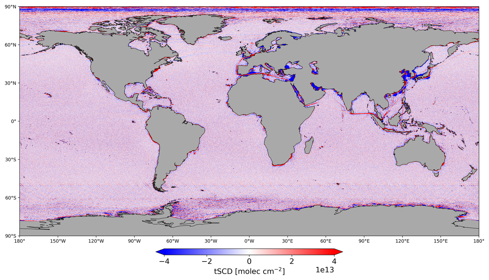
Figure B1 Same as Fig. 2 but with a symmetric color scale. This global map of filtered TROPOMI NO₂ tSCDs highlights the negative values (blue), which result from the high-pass filtering method and mainly occur at coastlines around Europe and Asia, including narrow regions like the Red Sea, the Persian Gulf, and the Yellow Sea.

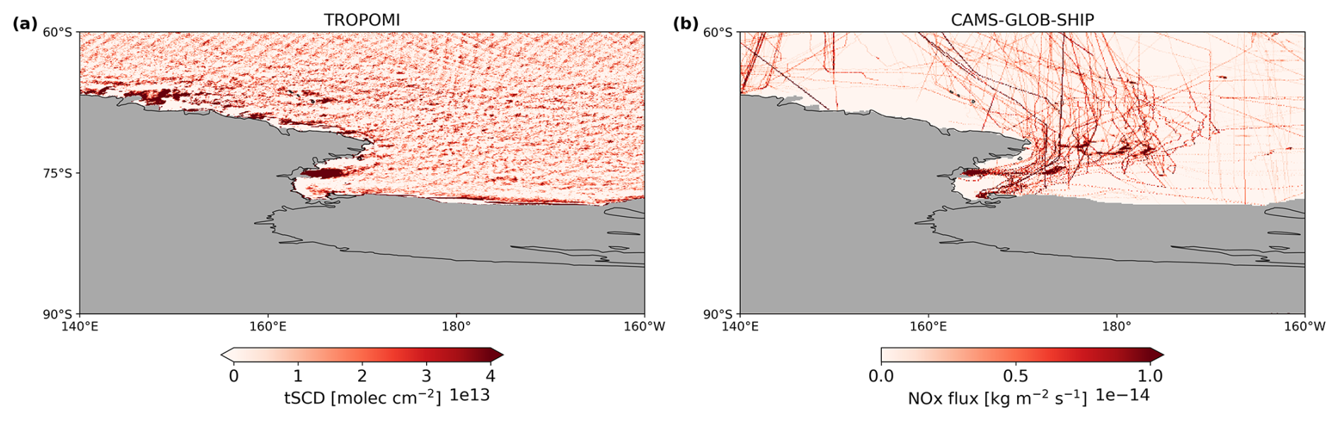
Figure B2 The higher NO₂ signal in the (a) filtered TROPOMI data in the Southern Ocean near the Antarctic continent can be assigned to (b) CAMS-GLOB-SHIP NO₂ shipping activities in the Ross Sea. The CAMS-GLOB-SHIP data cover the years from 2018 to 2021 (ECCAD, 2018). The enhanced NO₂ signal is detected only in the summer season with minimal sea ice extent, while during winter, the NO₂ signal in the Antarctic region is dominated by sea ice cover, indicating that these NO₂ emissions may originate from ship emissions.

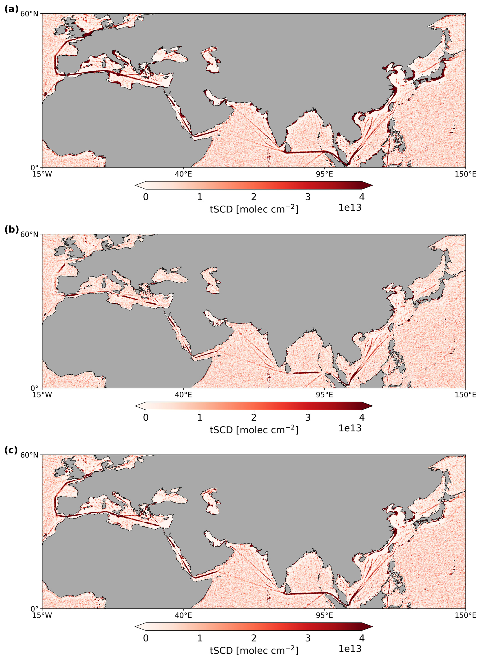
Figure B3 The region around the seas of Europe, Africa, and Asia with (a) the standard box size of 1° compared to (b) and (c) the individual box size approach, using two different box sizes depending on the distance from the coastline. The smaller box size of 0.25° is used for coastal pixels within (b) 50 pixels (≈ 1.5°) or (c) 17 pixels (≈ 0.5°), while the box size of 1° is used for all other pixels that are outside these coastal thresholds. One main advantage of this method is the reduction in high-pass filter effects near the coast. However, depending on the coastal threshold used, on a global scale, (b) visible shipping lanes, such as in the Mediterranean Sea, are also reduced, or (c) signals in narrow regions, such as the Persian Gulf, remain undetected.

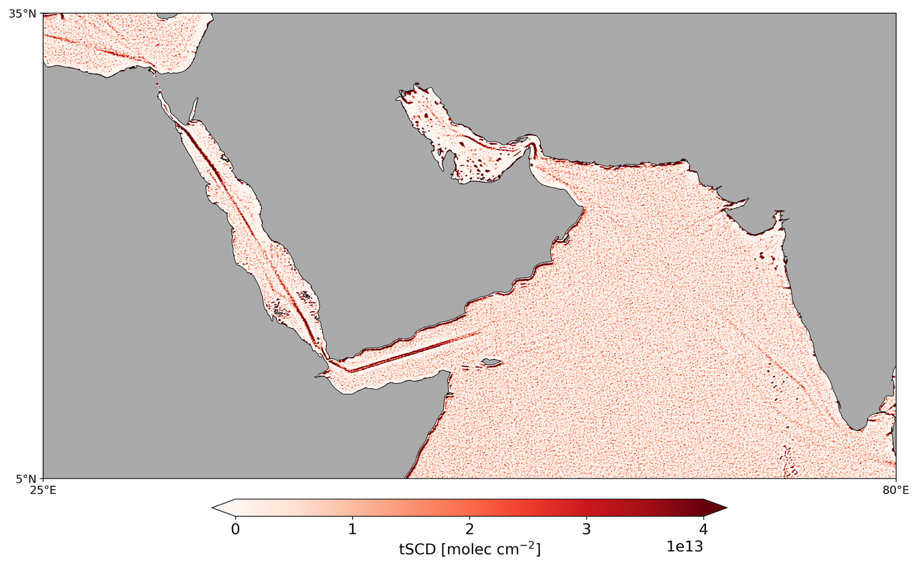
Figure B4 Filtered TROPOMI NO₂ signals from shipping activity in the Red and Arabian seas with the non-iterative high-pass filtering at a box size of approximately 0.25° in both longitude and latitude. Two separated shipping lanes are visible in the Gulf of Aden. In the Persian Gulf, a distinct shipping route is visible near the coast of Iran, and the dot-shaped elevated NO₂ values indicate NO_x emissions from offshore platforms. However, the shipping NO₂ signals in the Arabian Sea are not as pronounced as in the filtered TROPOMI data using the iterative approach with a box size of 1° (see Fig. 4a).

Appendix C: Additional comparisons between the filtered TROPOMI NO₂ data and the CAMS model

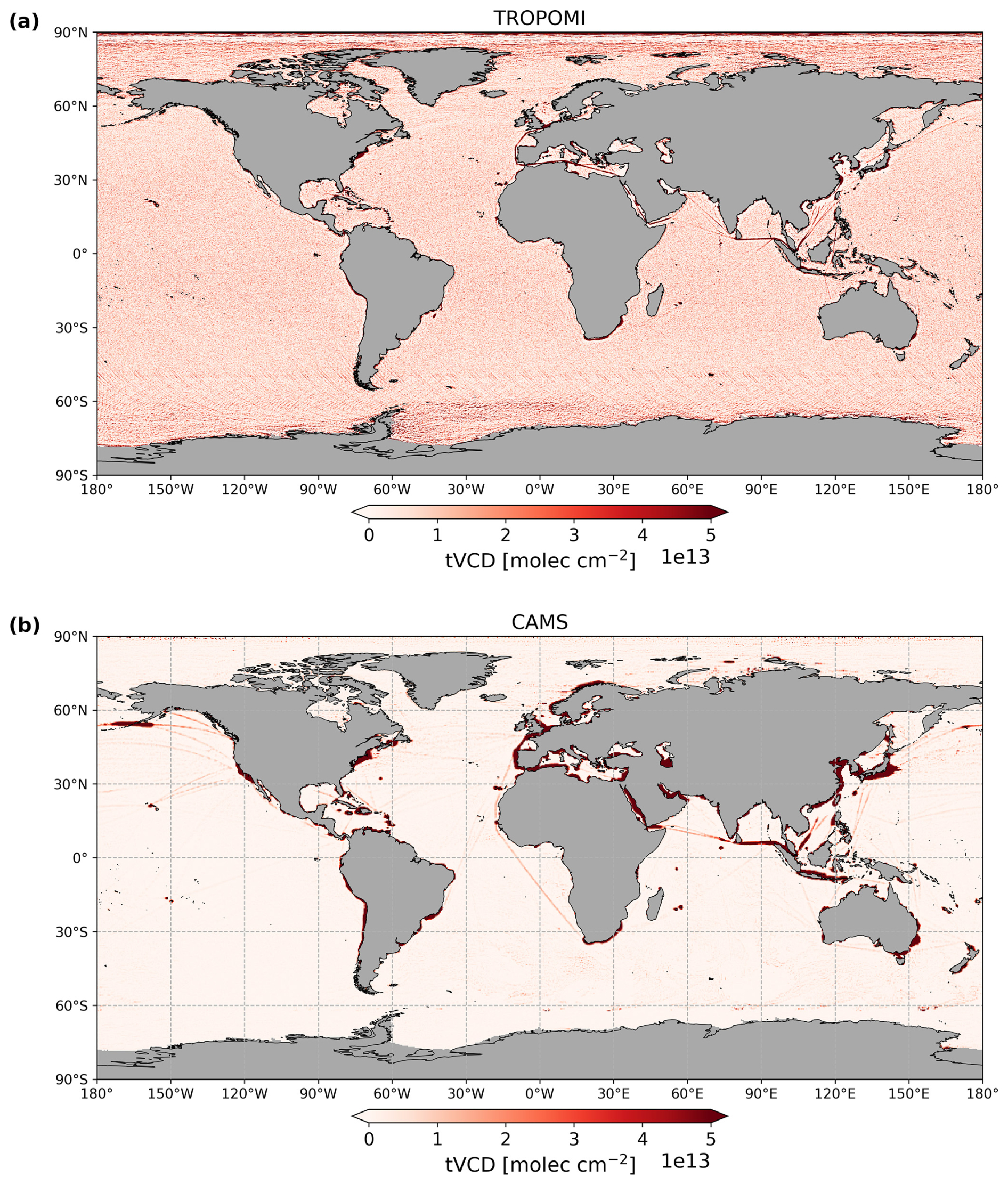
Figure C1 On a global scale, the positions of a large number of shipping routes, identified in (a) the filtered TROPOMI NO₂ tVCDs, are visible in (b) the high-pass-filtered CAMS NO₂ tVCDs. However, differences are found in the spatial extent of the shipping lanes, resulting from the coarser resolution of the CAMS model data, which are retrieved on a 0.4° × 0.4° grid from 2019 to 2023 with cloud flagging. The high-pass-filtered CAMS model data show a higher NO₂ signal in the Ross Sea near the Antarctic continent at a similar position to the filtered TROPOMI data (see also Fig. B2a), which confirms the assumption that this is an actual NO₂ emission signal.

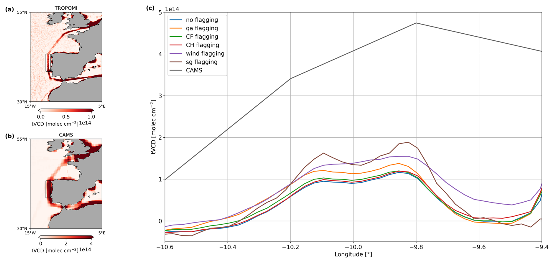
Figure C2 (a) Filtered TROPOMI NO₂ tVCDs with no flagging, (b) high-pass-filtered CAMS NO₂ tVCDs, and (c) the cross-sections of the shipping lane in the North Atlantic Ocean near the coast of Portugal (black rectangles) for the different TROPOMI flagging criteria and the CAMS model data. In addition to the at least 2 to 3 times larger CAMS NO₂ values compared to the TROPOMI data with different flagging criteria, the two peak patterns of this small-scale shipping lane are not as clearly identified in the CAMS curve as in the TROPOMI tVCDs due to the coarser resolution of the CAMS model data. In addition, this poor resolution leads to a mixing of shipping signals and emissions from land, here visible in the considerable NO₂ value at −9.4° longitude, which is not clearly set aside from the signal peak at −9.8° longitude.

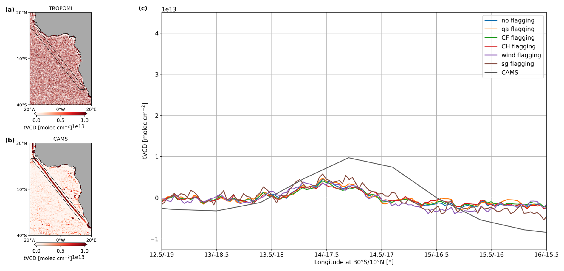
Figure C3 Same as Fig. C2 but (c) showing the cross-sections of the black polygons of the shipping lane in the South Atlantic Ocean west of the African continent. The high-pass-filtered CAMS NO₂ tVCDs capture the shipping lane with values twice as large as the filtered TROPOMI NO₂ tVCDs, which do not exceed 0.5 × 10¹³ molec. cm⁻² at the maximum peak. The filtered TROPOMI NO₂ curves vary greatly in this region due to the S5p orbit-oriented structures enhanced by the high-pass filtering, whereas the CAMS peak is straight-lined due to the coarser resolution. Constant background values in the CAMS model data and the resulting more pronounced shipping lane compared to the filtered TROPOMI data lead to smaller values on the sides of the CAMS curve, which shows a shifted peak compared to the TROPOMI peak, probably due to the coarser resolution of 0.4°.

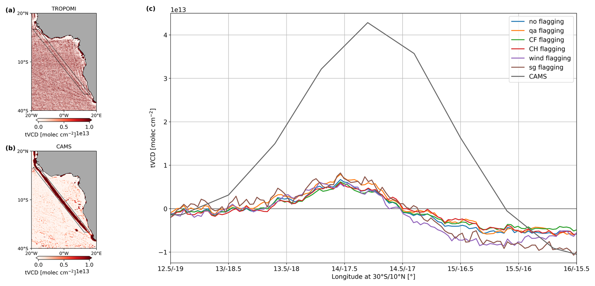
Figure C4 Same as Fig. C3, but the threshold for the masking in Step 2 of the high-pass filtering method is ±1 × 10¹³ molec. cm⁻² for both datasets. The filtered TROPOMI NO₂ tVCDs do not exceed 0.8 × 10¹³ molec. cm⁻² at the maximum peak and therefore show, as expected, only slightly higher peaks compared to those in Fig. C3c. In contrast, the high-pass-filtered CAMS NO₂ tVCDs strongly depend on the defined masking threshold and capture the shipping lane with more than 4 times larger values and a much broader FWHM compared to the CAMS curve with a threshold of ±3 × 10¹³ molec. cm⁻² (see Fig. C3c).