Validation and assessment of satellite-based columnar CO₂ and CH₄ mixing ratios from GOSAT and OCO-2 satellites over India

Satellite observations of column-averaged carbon dioxide (XCO₂) and methane (XCH₄) mixing ratios provide essential data for monitoring greenhouse gas (GHG) emissions. However, the accuracy of emission estimates depends on the precision and bias of satellite retrievals, which require validation against ground-based reference measurements. This study presents a systematic validation of XCO₂ and XCH₄ data from GOSAT (Greenhouse gases Observing SATellite) and OCO-2 (Oribiting Carbon Observatory-2) satellites over South India using ground-based Fourier transform spectrometer (FTS) observations at Gadanki (13.5° N, 79.2° E) collected from October 2015 to July 2016. Satellite products from National Institute for Environmental Studies, Japan (NIES), NASA's Atmospheric CO₂ Observations from Space (ACOS) project, USA (ACOS), and the University of Leicester, UK (UoL) were evaluated using a three-step spatial-temporal pairing method. Results show that the UoL's proxy XCH₄ product meets the European Space Agency's Climate Change Initiative (ESA CCI) bias requirement (<10 ppb) across all spatial windows, while the NIES XCH₄ product meets the requirement only for intermediate spatial scales. For XCO₂, NASA ACOS and OCO-2 products meet the CCI bias requirement (<0.5 ppm), while NIES XCO₂ exceeds this threshold. All products satisfy the precision requirement (<8 ppm for XCO₂ and <34 ppb for XCH₄) with substantial margins. In addition, FLEXPART model simulations using regional emission inventories revealed that agricultural activities dominate seasonal methane enhancements, contributing approximately 55 %, followed by waste and wetland emissions. The model captured seasonal trends but underestimated the amplitude of observed variations, highlighting the influence of changing background methane levels. These findings demonstrate the suitability of recent satellite products for regional GHG monitoring and emphasise the need for expanding ground-based FTS networks across South Asia to support improved emission assessments.

1 Introduction

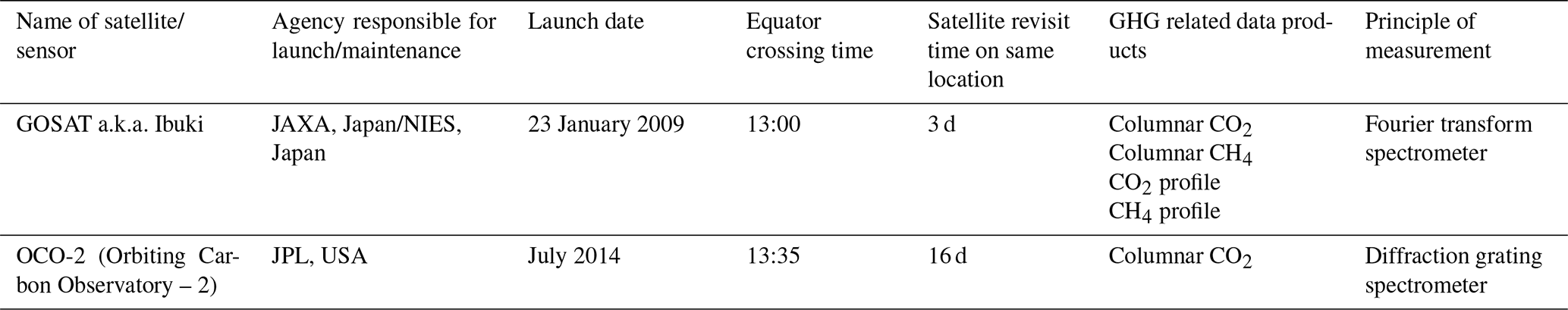
Carbon dioxide (CO₂) and methane (CH₄) are the two top most important greenhouse gases (GHGs) responsible for anthropogenic global warming. While the role of CH₄ in global warming is of primary interest, CH₄ also plays an important role in atmospheric chemistry by affecting OH amount, ozone production in remote areas and water (production) in the stratosphere (Fiore et al., 2002; Fleming et al., 2015; Laughner et al., 2021; Noël et al., 2018). Both CO₂ and CH₄ abundances in the atmosphere are on continuous rise post-industrial era (Dunn et al., 2022; Turner et al., 2019) and hence a continuous global monitoring of carbon dioxide and methane is highly desirable for identifying sources, sinks, trends and effective implementation of global treaties on reduction of GHGs by individual countries. Satellites, due to their continuously improving data products, have come to be recognised as important tools in the recent decade for monitoring and studying GHGs. Satellites such as GOSAT (Greenhouse gases Observing SATellite) and OCO-2 (Orbiting Carbon Observatory-2) capture scattered solar radiation in the near infrared spectral region and provide columnar mixing ratios. GOSAT and OCO-2 provide global coverage every 3 and 16 d, respectively (Table 1).

Table 1 Launch date, Equator crossing time, revisit time for global coverage and sensor technology of satellites, the data of which are used in the study.

Satellite based estimates of greenhouse and trace gases have proved effective for deriving the emission fluxes (Bergamaschi et al., 2007, 2009; Bousquet et al., 2011; Chevallier et al., 2005). However, the improvement that can be achieved in emission fluxes depends highly on the accuracy of satellite retrievals. The Climate Change Initiative (CCI) programme of the European Space Agency (ESA) has listed the threshold precision and systematic error requirements for satellite derived columnar CO₂ and CH₄ mixing ratios (henceforth, columnar mixing ratios of CO₂ and CH₄ are represented by symbols XCO₂ and XCH₄, respectively), which are <8 ppm precision and <0.5 ppm systematic error for XCO₂ individual measurements, and <34 ppb precision and <10 ppb systematic error for XCH₄ individual measurements for deriving the regional emission fluxes of these species (GHG-CCI, 2020). The World Meteorological Organization (WMO) Global Climate Observing System (GCOS) implementation plan has listed 1σ accuracy requirement of <0.5 ppm for XCO₂ and <5 ppb for XCH₄, respectively (GCOS-200, 2016).

To validate satellite-based estimates, standards against which the satellite observations can be compared are needed. The Total Carbon Column Observing Network (TCCON) operates high-resolution ground-based Fourier transform infrared spectrometers (FTSs) for providing column-averaged GHG abundances with high accuracy and precision. TCCON observations serve as the reference data source for satellite validation. Recently, TCCON was supplemented by portable FTS operated in the framework of the Collaborative Carbon Column Observing Network (COCCON). TCCON currently operates more than 20 stations worldwide for high-precision measurements of column average dry air mole fractions of CO₂, CH₄, N₂O, HF, CO, H₂O and HDO (https://tccon-wiki.caltech.edu, last access: September 2024). All the sites follow a common set of standards for instrumentation, data acquisition, calibration and analysis as prescribed by the TCCON steering committee. TCCON sites use IFS 125HR FTS manufactured by Bruker Optics which covers a spectral range from 3900 to 15 500 cm⁻¹ with a spectral resolution of 0.02 cm⁻¹. The calibration of TCCON is achieved using aircraft profiling over the sites. Errors in XCO₂ and XCH₄ are less than 0.16 % and 0.4 %, respectively, for solar zenith angle less than 82° (Laughner et al., 2024). While the XCO₂ and XCH₄ measured at TCCON sites are highly accurate and very important for validation of satellite, model and other instruments, the spectrometer is expensive, large and requires continuous maintenance. The IFS 125HR FTS dimensions are of the order of 1 m × 1 m × 3 m and weighs several 100 kg, restricting its widespread use or its deployment for short field campaigns or at remote sites with limited personnel. To supplement TCCON observations and to provide wider coverage of GHG observations, the Karlsruhe Institute of Technology (KIT) in collaboration with Bruker Optics, started developing a new type of portable FTS in 2011 which provides accurate measurement of GHGs while being lightweight and cost-effective. The prototype performance is described in Gisi et al. (2012). The spectrometer has become commercially available since 2014 under model designation EM27/SUN. Sha et al. (2020) compared the four different types of low-resolution spectrometers against IFS 125HR as well as in situ observations using AirCore from one of the TCCON sites over a period of 8 months and found EM27/SUN had the best performance matrix against high-resolution spectrometer. COCCON is an emerging network of the portable FTS which uses tested and calibrated EM27/SUN spectrometers as well as common algorithms for data processing (Alberti et al., 2022a; Frey et al., 2019; Sha et al., 2020). Support for calibration and data processing is provided by KIT and the COCCON spectrometers are calibrated against TCCON by performing side-by-side observations. Today, more than 83 EM27/SUN spectrometers are operated worldwide under the COCCON network (Alberti et al., 2022a). The portability of the EM27/SUN spectrometer and high accuracy in retrieving XCO₂ and XCH₄ have led to the instrument and COCCON network being used in a variety of applications. Mostafavi Pak et al. (2023) and Herkommer et al. (2024) have used the EM27/SUN spectrometer as travelling standard to evaluate consistency of TCCON measurements. Frausto-Vicencio et al. (2023) used the EM27/SUN spectrometer to estimate combustion efficiency of wild fires at regional scale. Stremme et al. (2023) used the spectrometer to study CO₂ plumes from a volcano. Dietrich et al. (2021) and Alberti et al. (2022b) used them for detecting city scale gradients in the gas mixing ratios and identifying the sources of emissions.

An assessment conducted by Buchwitz et al. (2017) using TCCON sites found that GOSAT and OCO-2 meet the requirements set by ESA's CCI Programme and WMO's GCOS implementation plan across various parts of the world. Due to a lack of data, this systematic assessment has so far not been conducted over South Asia; however, there have been studies that compared satellite data with ground-based FTS observations from Shadnagar (17°05^′ N, 78°13^′ E), near Hyderabad, Telangana – a city in the south-central part of India. Sagar et al. (2022) compared XCH₄ values from Sentinel-5P/TROPOMI (from December 2020 to March 2021) with ground-based FTS observations and found a mean bias of 3.61 ppb. Pathakoti et al. (2024) compared XCO₂ data from the OCO-2 satellite with ground-based FTS and reported a mean bias of 3.81 ppm and a root-mean-square error of 6.6 ppm. Pathakoti et al. (2024) used version 8 bias-corrected OCO-2 data. Aside from these few studies, no systematic ground validation of satellite data for GHGs has been conducted over the South Asian region. In addition, there has been no validation of GOSAT over South Asia. Since the release of version 8 of OCO-2 data, several improvements have been made to the OCO-2 algorithm, and the latest version (v11.1) is now available to public (Jacobs et al., 2024).

The National Atmospheric Research Laboratory (NARL), Gadanki and Institute for Meteorology and Climate Research (IMK-ASF) of KIT, Karlsruhe collaborated to make XCO₂ and XCH₄ measurements over South India using a portable FTS similar to the one used in the COCCON network. In this manuscript, we present a systematic validation of XCO₂ and XCH₄ estimated from GOSAT and OCO-2 over a site in South Asia using ground-based measurements and using the latest retrieval algorithms.

2 Instrumentation and data

In this study, a commercial low-resolution (0.5 cm⁻¹) FTS (Model: EM27/SUN FTS Make Bruker) with modified sun-tracker and InGaAs detector is used. The spectrometer has high thermal and mechanical stability and 0.5 cm⁻¹ spectral resolution in the spectral range 5000 to 9000 cm⁻¹. Sun-tracker system developed at KIT uses live sun image to guide sun-tracker for accurate position of sun-beam on the field stop. This allows far more precise sun-tracking even when intensity over the sun disc varies due to cloud or other factors. The tracking accuracy achieved is of the order of 11 arcsec (Gisi et al., 2011). A detailed description of the instrument can be found in Gisi et al. (2012). The instrument used has been calibrated by performing side-by-side measurements next to the TCCON spectrometer in Karlsruhe. The instrument is calibrated for specific deviations from nominal instrumental line shape (ILS) and the absence of any other systematic errors is verified at KIT. Details about the ILS measurement and data analysis as well as the comparison of calibration factors between the COCCON spectrometers have been discussed in Frey et al. (2019), Sha et al. (2020) and Alberti et al. (2022a). Sha et al. (2020) found a mean bias of −0.18 ± 0.45 and 0.003 ± 0.005 ppm between EM27/SUN and TCCON instrument for XCO₂ and XCH₄, respectively. The XCO₂ and XCH₄ scaling factors derived from side-by-side measurements between the spectrometer used in this study (Instrument Serial No. 52) and the COCCON reference spectrometer (Instrument Serial. No. 37) were determined to be 0.999482 and 1.000825, respectively, prior to the start of observations at Gadanki (Alberti et al., 2022a). In addition to solar spectra, measurements of atmospheric parameters such as temperature and pressure were also obtained near the spectrometer.

2.1 Ground-based FTS

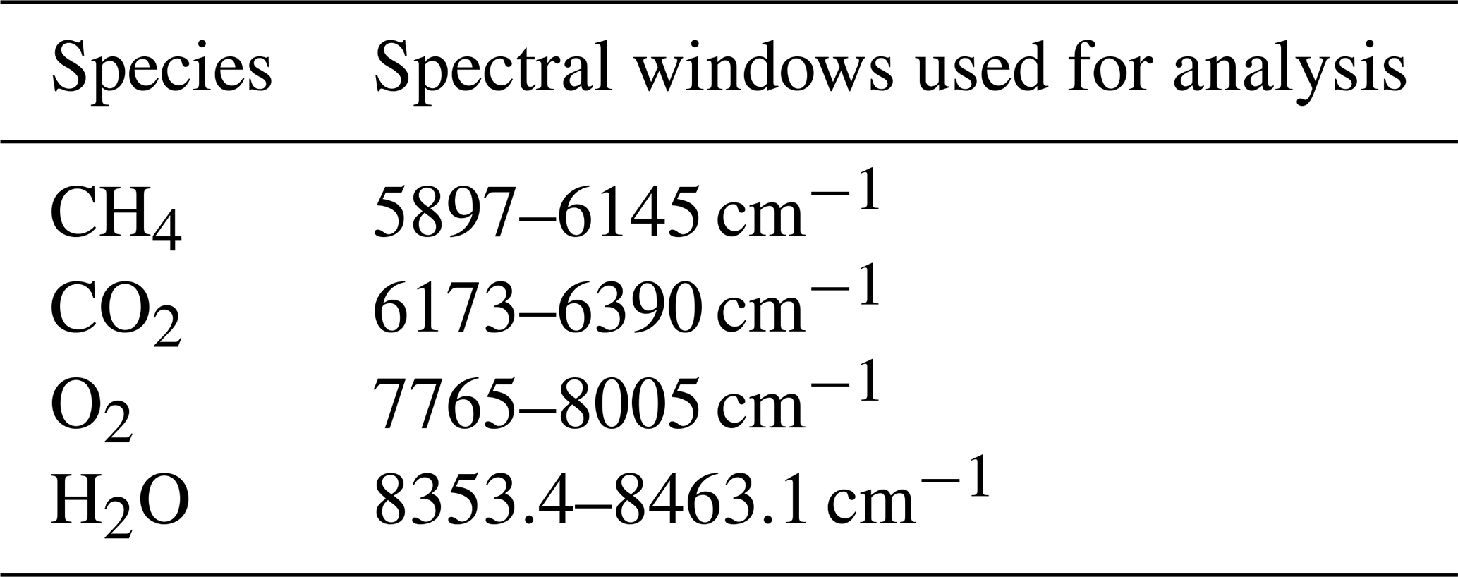
The recorded spectra are analysed using retrieval code PROFFAST v2.4 developed at KIT (KIT IMK-ASF, 2024a). PROFFAST software retrieves the gas amount by fitting solar absorption spectra and scaling a priori atmospheric profiles of the gases. It was run using a Python interface PROFFASTpylot v1.3 which also takes care of preprocessing of raw instrument data (Feld et al., 2024; KIT IMK-ASF, 2024b). The PROFFAST algorithm, which is a dedicated extension of PROFFIT Version 9.6 for processing of low-resolution spectra from spectrometers that are part of COCCON, is validated in several studies and used across all the COCCON sites to provide uniform and consistent data processing (Frey et al., 2019; Gisi et al., 2012; Hase et al., 2004; Sepúlveda et al., 2012; Sha et al., 2020). The spectral windows used for different species are listed in Table 2. The algorithm requires vertical profiles of temperature and pressure and a priori estimates of profiles of species to be estimated. Vertical profiles of temperature and pressure are obtained from National Center for Environmental Prediction (NCEP) reanalysis data corresponding to the dates of observations. The a priori estimates of species profiles are obtained from WACCM (Whole Atmosphere Community Climate Model) (Marsh et al., 2013) which is the average of 40-year monthly mean values for the site. The preprocessing step involves quality check of interferogram, DC correction, fast Fourier transform, phase correction and resampling of the spectra. Each record of raw data is a set of 10 spectra of which five are captured when the mirror is moving forward and five are captured when the mirror is moving backward. The interferogram is checked for signal level and source brightness fluctuations also known as DC variability and is removed from further analysis if threshold levels are not met. Other measurement and instrument specific corrections included in the processing are DC correction (correction for the sun brightness fluctuations) (Keppel-Aleks et al., 2007) and the application of ILS parameters (Abrams et al., 1994; Alberti et al., 2022a; Hase et al., 1999; Messerschmidt et al., 2010). As a first step, the columnar concentrations of CO₂, CH₄, O₂ and H₂O in terms of number of molecules per m² are retrieved. Then, the CO₂ and CH₄ concentrations are converted to column average mixing ratios by assuming O₂ mixing ratio as 20.95 % and normalising CO₂ and CH₄ concentrations with respect to O₂. This allows for compensating various systematic errors. XCO₂ measurement precision is 0.13 ppmv and XCH₄ measurement precision is 0.6 ppbv (Frey et al., 2019).

Table 2 List of spectral windows used for retrieving columnar concentrations of various gases using ground-based FTS.

Observations were carried out from October 2015 to July 2016 in the Gadanki campus of NARL. Gadanki (Latitude: 13.45° N, Longitude: 79.18° E, 360 m above mean sea level) is a rural site in South India with a tropical wet climate. It experiences two monsoon seasons known as southwest and northeast monsoon seasons. Change in wind circulation from one season to the other season is known to have significant effect on trace gases and aerosol concentrations at the site (Renuka et al., 2014, 2020; Sai Suman et al., 2014). The site is surrounded by hilly terrain and the nearest city is approximately 35 km away. A major part of the terrain surrounding Gadanki is forest and farm lands. Though there is no farming of rice (paddy field) in the immediate vicinity, the region as a whole has a good number of paddy fields. More details about the site and various atmospheric observation facilities can be found in Pandit et al. (2015) and Jayaraman et al. (2010). The FTS observations were carried out from morning to evening at intervals of 1 min except during days with inclement weather and weekends. More than 39 000 spectra covering a period of 10 months were analysed to retrieve XCO₂ and XCH₄.

2.2 GOSAT

The GHG observing satellite (GOSAT) also known as IBUKI is a joint project of the Ministry of the Environment (MoE), Japan, the National Institute for Environmental Studies (NIES), Japan and the Japan Aerospace Exploration Agency (JAXA), Japan (Yokota et al., 2009). The main instrument onboard GOSAT is a Thermal and Near infrared Sensor for carbon Observations (TANSO) (Table 1). It is a FTS with two detectors, one for shortwave infrared (SWIR) wavelength range and the other for thermal infrared (TIR) wavelength range (Olsen et al., 2017). While the TIR sensor is used to retrieve CO₂ and CH₄ profiles, the SWIR sensor is used to retrieve column average dry mole fraction of CO₂ (XCO₂) and CH₄ (XCH₄). In the current study, only XCO₂ and XCH₄ values from SWIR sensor are used.

The column-averaged dry-air mole fractions of methane (XCH₄) and carbon dioxide (XCO₂) retrieved from GOSAT are available from three different sources: (1) National Institute for Environmental Studies (NIES), Japan, (2) UK National Centre for Earth Observation at University of Leicester (UoL), UK and (3) the Goddard Earth Science Data Information and Services Center (GES DISC) of National Aeronautics and Space Administration (NASA, USA).

• NIES Data Products: NIES provides operational XCH₄ and XCO₂ products using a full physics algorithm, which minimises the difference between observed and simulated spectra generated by a radiative transfer model (Someya et al., 2023). In the current study, we use bias-corrected FTS SWIR Level 2 v3.05 data products from NIES, hereafter referred to as NIES XCH₄ or NIES XCO₂.

• UoL Data Products: UoL provides XCH₄ data derived using a proxy retrieval approach (Parker et al., 2020). This method first retrieves the ${\mathrm{XCH}}_{\mathrm{4}}/{\mathrm{XCO}}_{\mathrm{2}}$ ratio from the common absorption band near 1.6 µm, and then estimates XCH₄ by multiplying this ratio with a model-derived XCO₂ value. The advantage of this approach is its reduced sensitivity to aerosols, thin cirrus clouds and certain instrumental effects. However, reliance on model-based XCO₂ can introduce biases in the retrieved XCH₄. To mitigate this, UoL uses the median of XCO₂ estimates from three different atmospheric models constrained by surface in situ observations. In the current study, we use UoL Version 9 XCH₄ data, hereafter referred to as UoL XCH₄.

• NASA ACOS Data Products: NASA's GES DISC provides XCO₂ products retrieved under the Atmospheric CO₂ Observations from Space (ACOS) project (O'Dell et al., 2020), using a full physics algorithm originally developed for the OCO satellite and later adapted for GOSAT. In the current study, we use ACOS Level 2 bias-corrected XCO₂ Version 9.2 data, hereafter referred to as ACOS XCO₂.

2.3 OCO-2

The Orbiting Carbon Observatory-2 (OCO-2) is NASA's Earth remote sensing satellite to study atmospheric carbon dioxide from space (Crisp et al., 2004). In the current work, we have used processed and bias-corrected data version 11.1r downloaded from the website of GES DISC (http://disc.gsfc.nasa.gov/, last access: 26 August 2025). Version 11.1r is the latest version of data which were released in May 2023. The version 11.1r data contain retrospectively retrieved XCO₂ values using a full physics algorithm with several improvements with respect to its predecessor algorithms (Jacobs et al., 2024; Payne et al., 2025). The OCO-2 was launched on 2 July 2014 in sun-synchronous orbit with equatorial crossing time at 13:30 on an ascending node with a 16 d repeat cycle (Table 1). The OCO-2 instrument consists of three boresight high-resolution imaging grating spectrometers which provide high-resolution spectra of reflected sun light in oxygen A band (0.765 µm) and in two CO₂ bands at 1.61 and 2.06 µm. The instruments can be operated in three modes viz., target, glint and nadir. The ground resolution varies depending on the mode of operation. In the current study, data from the nadir mode are used which has a spatial resolution of 1.29 km × 2.25 km (Crisp et al., 2017). The spectra are corrected for various artefacts such as bad pixels, cosmic ray artefacts and converted to radiometric values. Using a full physics radiative transfer model, synthetic spectra are produced and compared with observed spectra. An inverse model iteratively modifies the assumed atmospheric state to improve the fit. The number densities of CO₂ and O₂ thus retrieved are used to get XCO₂ by taking their ratio and multiplying it by 0.2095. The retrieval is further enhanced with applied bias correction obtained from collocated TCCON data, models and small area analysis (O'Dell et al., 2018). More details of the retrieval process are available in Crisp et al. (2021). The OCO-2 data are distributed in two formats known as standard files and Lite files. The standard files contain CO₂ mixing ratios without bias correction, whereas mixing ratios in the Lite files are bias corrected (Payne et al., 2025). The data files contain a quality flag for each retrieval. The quality flag value “0” corresponds to good data, whereas the quality flag value “1” suggests the presence of any of the 24 algorithmically identified quality issues in the retrieved value. In the present work, we used bias corrected data with quality flag “0” only.

3 FLEXPART (A Lagrangian particle dispersion model)

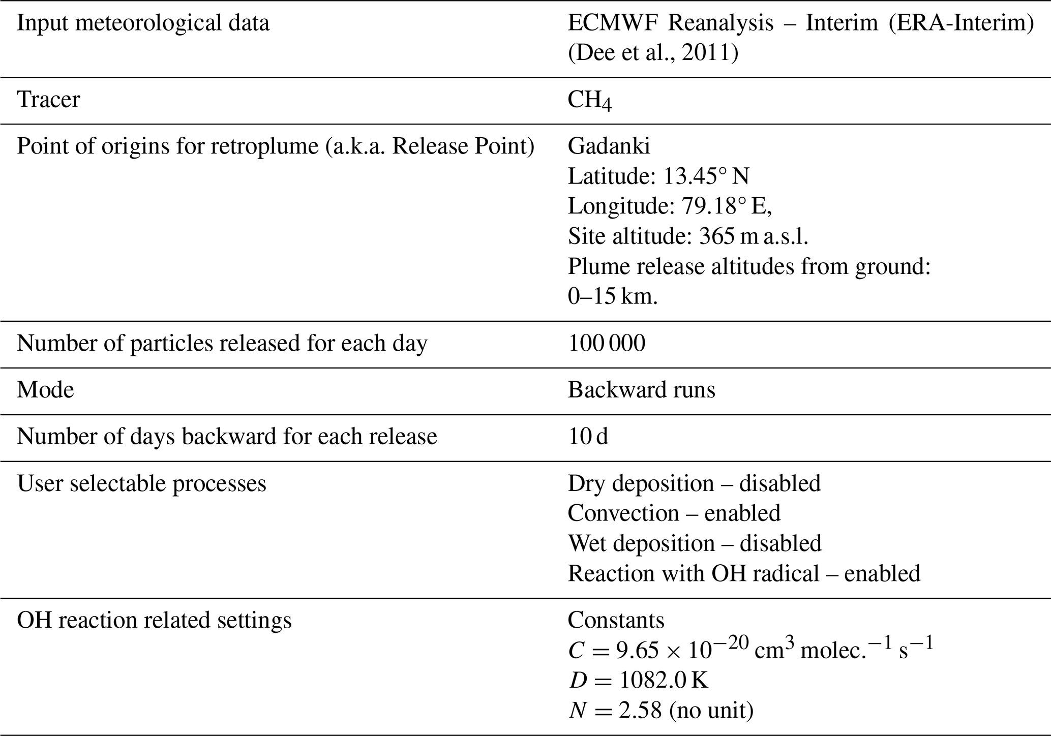
In comparing satellite data with ground-based observations, we also examined the seasonal variation of methane mixing ratios using a Lagrangian particle dispersion model to understand the influence of local sources vis-a-vis long-range transport. The FLEXPART (Pisso et al., 2019), an open-source model developed at the Norwegian Institute for Air Research (NILU), Kjeller, Norway is widely used by the research community around the world to identify the source regions of long range transport. The model takes meteorological fields as input and tracks the movement of virtual particles forward or backward in time. The particles can be configured to represent a gas or aerosols of one's choice and accordingly be subjected to various physical processes such as advection, turbulence, dry deposition, wet deposition, radioactive decay, etc. Except for reaction with OH radical no other chemical transformation is modelled in FLEXPART.

We configured FLEXPART for backward-in-time runs from the observation site (Gadanki) with virtual particles representing methane molecules. The backward-in-time runs provide a source-receptor relationship which can be used to calculate mixing ratios or concentrations at the observation site using emission fluxes. The model run is configured such that mixing ratios thus calculated represent results of emissions within the past 10 d for an average of 0 to 15 km atmospheric column at the observation site. This configuration effectively captures most regional emissions and tropospheric methane mixing ratios. Using few sensitivity tests, we found that emissions within 10 to 15 d have insignificant contribution to concentrations beyond 15 km. More details of the model settings used for the current study are listed in Table 3.

Table 3 The FLEXPART model setup and the input data details.

3.1 ECLIPSEv6 inventory

To calculate the concentrations resulting from recent regional emissions (emissions within past 10 d of a given observation), we used ECLIPSEv6b (Evaluating the CLimate and air quality ImPacts of Short-livEd pollutants version 6b) emission inventory (Amann et al., 2011, 2012; Klimont et al., 2017; Höglund-Isaksson, 2012; Stohl et al., 2015). The inventory is prepared following the IPCC (2006) recommended method and using the Greenhouse Gas – Air Pollution Interactions and Synergies (GAINS) model (Amann et al., 2011). It provides sector-specific anthropogenic emission estimates for 11 species, including CH₄, across eight economic sectors. The data are provided as 0.5° × 0.5° gridded values for the years from 1990 to 2050 at an interval of 5 years for two scenarios – the current legislation for air pollution – which is also the reference scenario and maximum technically feasible reductions scenario. The latest version (Version 6b) was released in August 2019 and incorporates updates for historical data, new waste sectors, soil NO_X emissions, international shipping emissions and energy-macroeconomic data. The inventory includes only anthropogenic emission fluxes from sectors; viz. energy, industry, solvent use, transport, domestic combustion, agriculture, open biomass and agricultural waste burning and waste treatment. Natural emissions from wetlands, forest fires, biogenic emissions, etc. are not included in the inventory. The total Global, South Asia (members of SAARC – South Asian Association for Regional Cooperation), and India's emissions of methane for the year 2015 were 336.2, 44.2 and 31.5 Tg, respectively.

3.2 Wetland inventory

The emissions from wetlands can contribute significant atmospheric load of methane at the observation site and hence in addition to anthropogenic emissions from ECLIPSEv6 inventory, we used Wetland CH₄ emissions and uncertainty dataset for atmospheric chemical transport models (WetCHARTs) version 1.0 inventory (Bloom et al., 2017a, b) for calculating methane concentrations at Gadanki from recent emissions. The inventory contains global monthly emission fluxes of methane at 0.5° by 0.5° resolution for ensemble of multiple terrestrial biosphere models, wetland extent scenarios and temperature dependencies. The emission fluxes from 2001–2015 are provided for three choices of global scaling, two choices of wetland spatial extent, two choices for temporal variability of wetland extent, nine choices of heterotrophic respiration schemes and three choices of parameterisation scheme for temperature dependency. In the current work, we used data corresponding to the scaling factor with global emissions 166 TgCH₄ yr⁻¹, CARDAMOM (CARbon DAta MOdel fraMework) terrestrial C cycle analysis for heterotrophic respiration (Bloom et al., 2016), mid-range temperature sensitivity and, spatial and temporal extent of wetlands constrained with SWAMPS (Surface WAter Microwave Product Series) multi-satellite surface water product (Schroeder et al., 2015). These choices were made based on following consideration. Choice of scaling factor represents the mid-point global emissions among the three choices available, viz. 124.5, 166 and 207.5 Tg CH₄ yr⁻¹. While there are nine choices for heterotrophic respiration, there is only one choice available for emission fluxes after 2010 which is CARDAMOM and used here. Between the two choices of spatial extent and two choices of temporal variability, the SWAMPS multi-satellite surface water product is used because it represents observationally constrained inundated areas including lakes and other water bodies.

4 Results and discussion

Box plots of monthly statistics are shown in Fig. 1 for (a) XCH₄ and (b) XCO₂ measured by EM27/SUN at the Gadanki site. Figure 2 shows the time series of hourly mean values of XCH₄ and XCO₂ from EM27/SUN, NIES, UoL, ACOS and OCO-2 within box size ±30° longitude and ±10° latitude of the site (Table 4). A large variability in XCH₄ values is observed in October, but in other months, the variability is relatively low. The median values of XCH₄ are found to systematically decrease from 1.892 ppm in October to 1.826 ppm in June of the following year, with similar values observed in July. The monthly median values of XCO₂ increased from 396.4 ppm in October to 405.8 ppm in May, then began to decrease after May. Unlike XCH₄, the XCO₂ values did not show high variability in October. A similar seasonal variation was observed by Jain et al. (2021) in surface mixing ratios of CO₂ and CH₄ at Gadanki. Kavitha and Nair (2016) using SCIAMACHY satellite data over India for the period 2003–2009, also reported similar seasonal variations, attributing them to regional rice cultivation patterns. Further discussion on the seasonal variation is provided in the subsequent section.

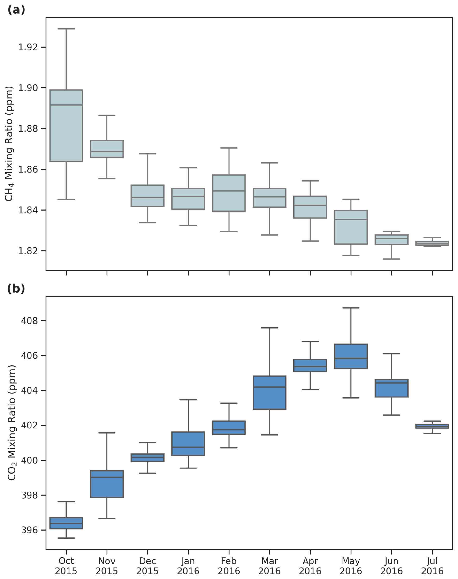
Figure 1 Box plot of monthly statistics of (a) CH₄ and (b) CO₂ columnar mixing ratios observed at Gadanki, India using ground-based FTIR.

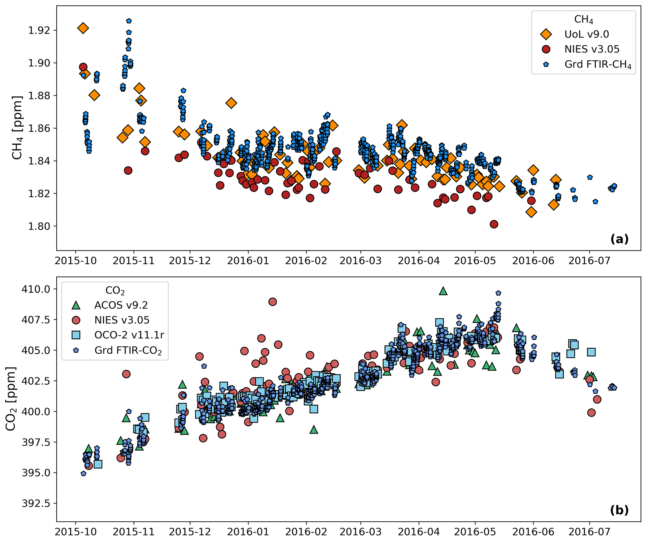
Figure 2 Hourly mean values of columnar CH₄ (a) and CO₂ (b) mixing ratios observed using ground based FTIR along with paired satellite observations. See the text for description of pairing method (Box size ±30° longitude and ±10° latitude).

4.1 Comparison of satellite-based and ground-based mixing ratios

The GOSAT satellite revisits the same point on Earth every 3 d, with retrievals performed only under cloud-free sky conditions. This limits the number of concurrent satellite and ground-based FTIR measurements. To address this limitation and ensure sufficient data pairs for comparison, we followed an approach similar to Buchwitz et al. (2017). This approach relies on the fact that CO₂ and CH₄ have long atmospheric residence times, allowing the history of air parcels to be used to pair data for comparison.

In this approach, the first step is to identify all satellite data within a certain distance of the ground station. Buchwitz et al. (2017) used satellite data within ±30° longitude and ±10° latitude of TCCON sites to evaluate GOSAT and OCO-2 data products. Wunch et al. (2017) used box of ±5° longitude and ±2.5° latitude around the TCCON sites in the Northern Hemisphere and ±60° longitude and ±10° latitude around the TCCON sites in the Southern Hemisphere to evaluate XCO₂ estimates from the OCO-2 satellite. In the second step, ground-based observations taken within 3 d of the satellite overpass and during same time of the day (within 2 h) are paired with the satellite data. In the third step, the data pairs obtained in step 2 are further filtered using the criterion that the CAMS model output of XCH₄ and XCO₂ values, interpolated to the satellite location and ground station, cannot differ by more than 0.25 ppm for XCO₂ and 5 ppb for XCH₄, respectively. This third step is based on the premise that the CAMS model is capable of simulating transport accurately, meaning that while the absolute values may not always be correct, the spatial variability in the model is reliable. The criteria in step 3 ensures that satellite and ground values are only compared when they share the same air mass history. Note that the absolute value of the model simulation and its differences with observations are not relevant in this step. More detailed discussions on the need and the rationale behind this complex approach for data pairing can be found in Nguyen et al. (2014) and Wunch et al. (2011). A sensitivity test, described in Table S1 of the Supplement, shows omitting the model-based air mass filtering (step 3) increases the number of matched pairs by factors of 2–3 across species and datasets. While the effect on bias is mixed, the scatter generally increases slightly when step 3 is not applied. For consistency with previous studies, we report results based on the full three-step pairing procedure.

We note that no averaging kernel (AK) correction were applied in this analysis. While applying AK corrections is ideal to account for vertical sensitivity differences between satellite and ground-based retrievals, the effect of their omission is expected to be small for our study location. Sha et al. (2021) demonstrated that at low-latitude sites, the effect of smoothing and a priori profile differences on XCH₄ biases is minor, typically below −0.25 %, with an average effect of −0.14 %. Given that Gadanki (13.5° N) is a low-latitude station, the lack of AK correction is unlikely to significantly affect our conclusions.

We performed calculations for three different box sizes around the observation site at Gadanki (13.45° N, 79.18° E): (±5° longitude, ±2.5° latitude), (±10° longitude, ±5° latitude), and (±30° longitude, ±10° latitude). By the end of the third step, we obtained 55 pairs of XCH₄ from GOSAT NIES v3.05, 81 pairs of XCH₄ from GOSAT UoL v9, 117 pairs of XCO₂ from GOSAT v3.05, 117 pairs of XCO₂ from ACOS v9.2 and 120 pairs of XCO₂ from OCO-2 v11.1 for the biggest box size in step 1 (see Table 4, Fig. 2). The number of data pairs for XCO₂ is more than double that of XCH₄ for all box sizes. This difference reflects the fact that carbon dioxide has a much longer atmospheric lifetime (>100 years) compared to methane (∼ 12 years).

Table 4 Mean bias and scatter between satellite and ground-based measurements. Values that meet CCI criteria are shown in bold letters.

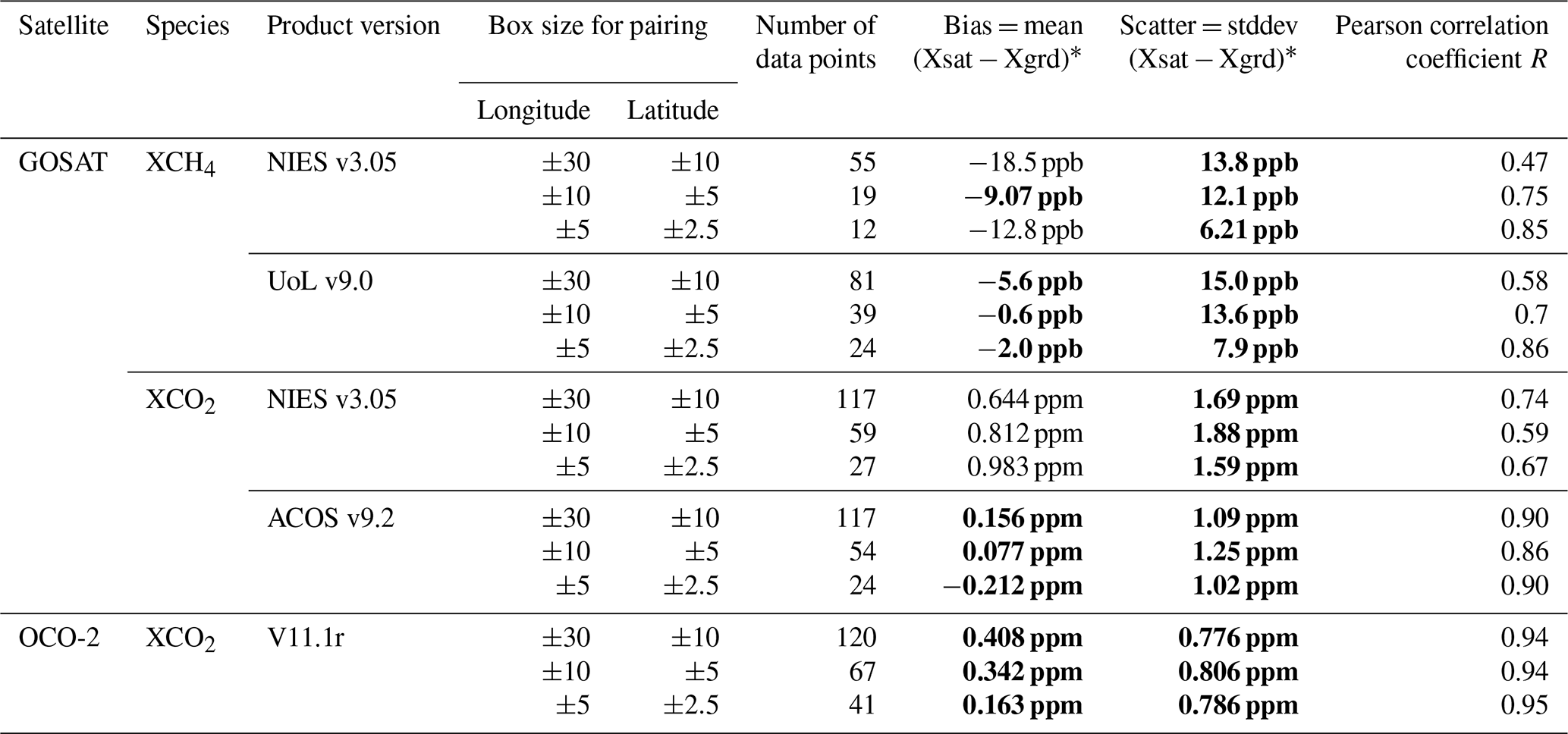
^* Xsat are satellite based mixing ratio estimates and Xgrd are ground based FTIR mixing ratio estimates. For all the satellites, their bias corrected values are used.

With the paired dataset in place, we evaluated the bias, scatter and correlation between satellite and ground-based measurements, as listed in Table 4. Here, bias is defined as the mean of difference between satellite- and the ground-based dry-air mole fractions; scatter as the standard deviation of these differences; correlation as the Pearson correlation coefficient (R) between the paired values. The European Space Agency's Climate Change Initiative (ESA CCI) specifies performance targets of <34 ppb for scatter (precision) and <10 ppb for bias (systematic error) for XCH₄, and <8 ppm for scatter and <0.5 ppm for bias for XCO₂ (GHG-CCI, 2020).

4.1.1 XCH₄ validation results

For GOSAT NIES XCH₄, biases ranged from −9 to −18.5 ppb depending on the spatial window size. For GOSAT UoL XCH₄, biases were notably lower, ranging from −0.6 to −5.6 ppb. While larger spatial windows provided more matched pairs, they did not consistently yield lower bias or scatter. In fact, the intermediate box size (±10° × ±5°) showed the lowest bias and scatter for both products. Importantly, biases across all box sizes remained within one standard deviation of the smallest box size, indicating that larger spatial windows may not offer significant additional value, particularly when longer time series of ground-based data are available.

The UoL XCH₄ product met the ESA CCI bias requirement (<10 ppb) across all box sizes. In contrast, the NIES XCH₄ products met this requirement only for the intermediate box, with marginal exceedances for the smallest box. Scatter values ranged from 6 to 15 ppb across products and box sizes, well within the CCI precision requirement of 34 ppb.

Although derived from the same satellite, the UoL XCH₄ product, which uses a proxy retrieval approach, showed substantially improved bias performance compared to the NIES product. However, its scatter was slightly higher (approx. 2 ppb) than the NIES product for equivalent spatial windows ranging from 8 to 15 ppb.

4.1.2 XCO₂ validation results

All XCO₂ products showed high correlation with ground-based measurements across all spatial windows. Biases for GOSAT NIES XCO₂ ranged from 0.644 to 0.983 ppm, exceeding the CCI bias threshold of 0.5 ppm for all box sizes. However, scatter values (1.59–1.88 ppm) were well below the 8 ppm precision requirement.

In contrast, ACOS v9.2 XCO₂, also based on GOSAT observations but using a different retrieval algorithm, demonstrated superior performance. Biases ranged from −0.212 to 0.163 ppm, meeting the CCI bias requirement across all box sizes. Scatter ranged from 1.02 to 1.25 ppm, also comfortably within the precision target. Correlation coefficients (R=0.86–0.90) for ACOS XCO₂ were higher than those for NIES XCO₂ (R=0.59–0.74).

The OCO-2 XCO₂ v11.1r product showed the highest correlation among all datasets (R=0.94–0.95), with biases ranging from 0.163 to 0.408 ppm, fully meeting the CCI bias target. Scatter values (0.776–0.806 ppm) were the lowest among all products evaluated.

Our results for OCO-2 XCO₂ differ notably from the higher bias of 3.81 ppm reported by Pathakoti et al. (2024) for Shadnagar, India, located approximately 500 km north of our study site. While Pathakoti et al. have not discussed the reason for such a high bias in their study, it is unlikely to be solely due to the use of an earlier version of the OCO-2 dataset by them. Pairing methodology differences between our study and that of Pathakoti et al. may have contributed to the difference in results. Their study used a smaller spatial window (4° × 4°) and daily mean ground-based values, whereas we applied a larger spatial window (10° × 5°), used hourly collocation within ±2 h, and applied model-based air mass filtering to improve representativeness. Additionally, Pathakoti et al. did not specify the retrieval algorithm version for their ground-based FTS data. Mostafavi Pak et al. (2023) have shown that using retrieval algorithm GGG2020 instead of GGG2014 reduces XCO₂ bias from 1.3 to 0.5 ppm, which may further explain the discrepancy.

Figure 3 shows the time series of XCH₄ and XCO₂ biases for the ±30° × ±10° box. No systematic changes in biases are observed for most products, except for GOSAT NIES XCO₂, values which exhibited positive biases during December to February and negative biases during April to May. Overall, the biases at the Gadanki are consistent with those reported by O'Dell et al. (2018) for OCO-2 version 8 over TCCON sites (∼ 1 ppm).

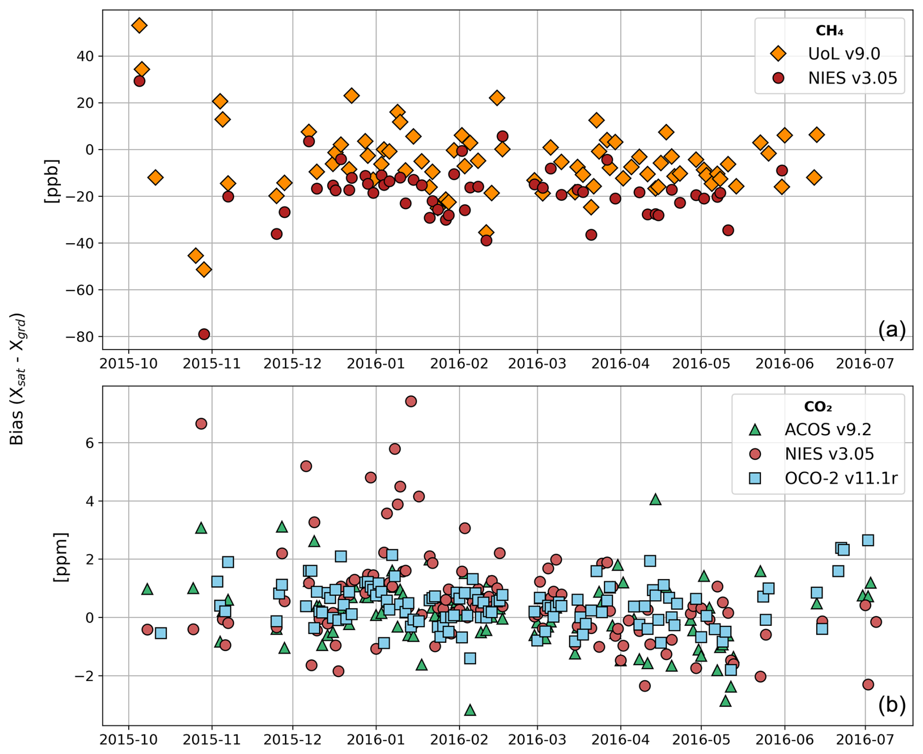
Figure 3 Time series of biases in GOSAT and OCO-2 retrieved XCH₄ (a) and XCO₂ (b) over Gadanki, India. Results are shown for satellite data selected within a ±30° longitude × ±10° latitude region centred on the station.

4.2 Case studies and seasonal variations of methane

Figure 4 shows methane mixing ratio enhancements calculated using the FLEXPART model and the ECLIPSEv6 + Wetland inventory. As previously mentioned, the model is configured such that the values represent daytime mean mixing ratios in the altitude range of 0 to 15 km over Gadanki, contributed by emissions from the preceding 10 d. The altitude range of 0 to 15 km is selected because the tropopause altitude in the tropics is typically between 15 and 18 km (Pandit et al., 2014), and emissions from the past 10 d are generally confined within this range.

The 10 d back trajectory is chosen based on earlier work by Gadhavi et al. (2015), which demonstrated that, for the Gadanki location, a 10 d back trajectory captures emissions from almost the entire South Asia. The averaging period is selected as daytime (9 am to 6 pm local time) to ensure a one-to-one correspondence with observed mixing ratios, which are measured using solar radiation through FTS and are therefore only available during daylight hours.

Hereafter, these values will be referred to as model values, However, it is important to note that the model values do not account for the columnar CH₄ mixing ratio resulting from emissions prior to the 10 d period and, therefore, do not represent the total columnar mixing ratio as seen in FTS or satellite data.

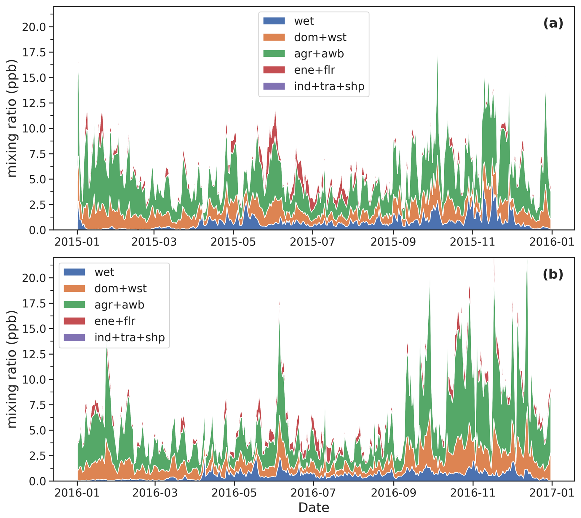
Figure 4 Model calculated columnar (0 to 15 km) average methane mixing ratio enhancements due to emissions of past 10 d for year (a) 2015 and (b) 2016. Colours show contribution of different sectors viz. wetland (wet), domestic + waste (dom + wst), agriculture  +  agricultural waste burning (agr + awb), energy  +  flaring (ene + flr), and industry  +  transport  +  shipping (ind + tra + shp).

Overall, the model estimates methane mixing ratio enhancements ranging from 2 to 26 ppb during 2015 and 2016. While there is significant day-to-day variability, a seasonal pattern is still discernible in the model-calculated values. Typically, the mixing ratio enhancements are high in November, decrease slightly in December, and rise again during January and February. They decrease in March and April, briefly rise in the second half of May, and then decrease again, remaining low from June to September. The mixing ratios rise again in October, peaking in November. Sector-wise, wetlands do not show large seasonal variations. Wetland contributions are low from December to March. In other seasons, wetland contributions occasionally reach as high as 40 % of total mixing ratios, but for most part of the year, they remain around 10 %. The highest contribution comes from the agriculture sector, accounting for nearly 55 % of the total mixing ratio enhancements, followed by the waste sector, which contributes approximately 17 % to the model values at Gadanki. The domestic and energy sectors contribute approximately 5 % each. The domestic sector's contribution is lower in July and August, mainly due to the air masses originating from the west of Gadanki in peninsular India, where the population is smaller and contributes less to methane emissions. Flaring contributes negligibly for most part of the year, but during June to July, its contribution can reach up to 40 %, primarily due to low emissions from other sectors during this period and the winds from the Arabian Sea bringing emissions from oil rigs off the west coast of India, the eastern Arabian Peninsula, and northeastern Africa. Industry, transport, shipping and agricultural waste burning activities contribute less than 1 % of atmospheric load of methane at Gadanki.

Figure 5 shows model-calculated methane mixing ratio (ΔXCH₄; solid blue line; left y axis) and the methane mixing ratios (XCH₄) observed using FTS (red filled circles; right y axis) in a single plot. The left-hand side y axis represents the model mixing ratio, which only accounts for emissions from the preceding 10 d. For lack of a better term, we refer to it as ΔXCH₄. The right-hand side y axis shows the observed values in ppm. As mentioned earlier, the model was configured to reflect incremental variability caused by regional emissions. If the background CH₄ mixing ratios were constant, the day-to-day variability relative to background values should be the same in both the model and the observations. However, we observe differences in both the absolute values of variability and their seasonal patterns. Several sudden increases in the model values, which appear as spikes in Fig. 5 (e.g. 5 October and 27 December 2015), correspond to variations in the observations. While the observations are not as continuous as model values and cannot capture all the variability seen in the model, some degree of day-to-day variability is correlated between the model and observations (R²=0.35). However, the magnitude of variability between the model and observed values is quite different. For instance, the observed mixing ratios from 5 to 8 October 2015 decreased by 49 ppb, whereas the model values during the same period decreased only by 16 ppb. Over the entire observation period, total column methane mixing ratios varied by 100 ppb, while the model values which excludes background mixing ratios varied only by 20 ppb. This discrepancy may be due to two main factors: either the emission fluxes in the emission inventory are underestimated, or the background mixing ratios are not constant. The latter factor could explain the mismatch on a monthly scale. Starting in October 2015, both model and observed values are high and decrease toward June–July 2016. While the model values are already low by March 2016, the observed values decrease gradually from November 2015 to January 2016, remain nearly constant from January 2016 to April 2016, and then decrease rapidly in May, reaching a minimum during the last week of June and the first week of July.

Chandra et al. (2017) analysed methane variations over different parts of India using the Japan Agency for Marine-earth Science and TEChnology (JAMSTEC) Atmospheric Chemical Transport Model. They found that, over South India, although 60 % of the columnar concentration is attributed to CH₄ in the lower troposphere, there is very little correlation between regional emissions and columnar methane variations. This was attributed to changes in atmospheric chemistry and transport. According to Chandra et al. (2017), the methane loss rate increases from 6 ppb d⁻¹ in January to 12 ppb d⁻¹ from April to September. In addition, anticyclonic winds in the upper troposphere confine uplifted methane molecules over broader South Asia during the monsoon season, contributing significantly to methane over Western India, but not significantly over South India. Since FLEXPART does not include chemistry other than the reaction with OH radical, a lower decrease in model values from March to July could be due to absence of chemistry as well as transport of background methane.

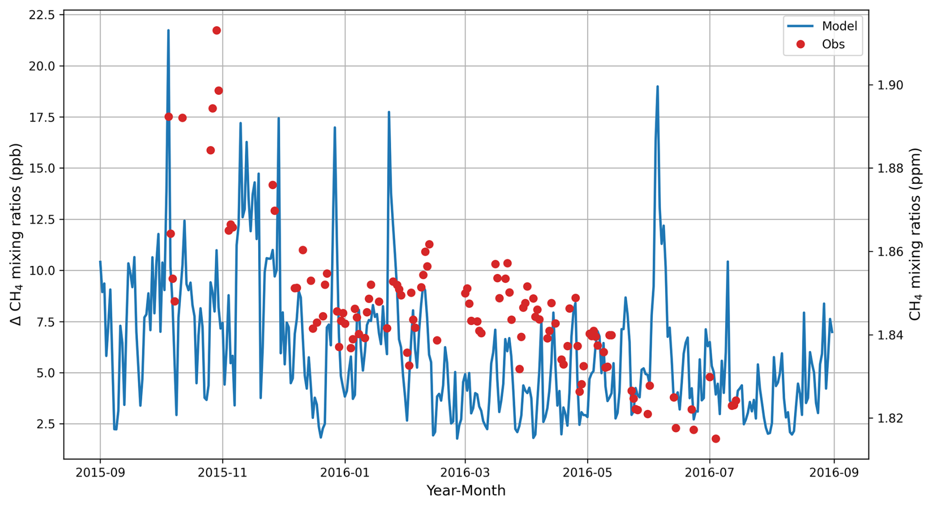
Figure 5 Observed and modelled mixing ratios at Gadanki. (The left-hand y axis shows value for modelled mixing ratio and right-hand axis shows value for observed mixing ratios.)

5 Conclusions and outlook

The GOSAT and OCO-2 satellites provide global coverage of columnar mixing ratios of CO₂ and CH₄ every 3 and 16 d, respectively. These data are crucial for deriving regional greenhouse gas emission fluxes. However, the accuracy of the derived emission fluxes strongly depends on the precision and accuracy of the satellite products. In our study, we compared GOSAT and OCO-2 satellite-measured columnar mixing ratios of CO₂ and CH₄ with ground-based FTS measurements from a location in South India.

The biases in methane mixing ratios estimated using the GOSAT satellite ranged from −0.6 to −18.5 ppb, depending on the product and matching criteria used for the collocation of ground and satellite footprints. Even though NIES and UoL XCH₄ dry-air mole fractions were derived from the same satellite (GOSAT), UoL XCH₄ data have much smaller biases for corresponding spatial box sizes. The biases in UoL XCH₄ meet ESA's CCI requirement for systematic errors (<10 ppb) for all the matching criteria, NIES XCH₄ meet the requirement only for intermediate longitude–latitude box size. Both the products meet precision requirement (<34 ppb) with NIES XCH₄ having slightly better performance irrespective of longitude–latitude box size.

Again, NIES XCO₂ and ACOS XCO₂ products are derived from the same satellite (GOSAT); the NIES XCO₂ product does not meet the CCI's systematic error requirement of <0.5 ppm, whereas ACOS XCO₂ data product not only met the CCI's systematic error requirement, it had the lowest biases among the three XCO₂ datasets evaluated. Both the ACOS and OCO-2 data meet ESA's CCI requirement for CO₂ biases (<0.5 ppm), while the NIES XCO₂ v3.05 values showed higher biases, ranging from 0.644 to 0.983 ppm. The precision requirement of <8 ppm for XCO₂ set by ESA CCI was met by all three datasets with a significant margin, with scatter values ranging from 0.776 to 1.88 ppm.

We used model to understand seasonal changes resulting from local and regional emissions in methane mixing ratios and sectoral composition of the sources. The model captures the overall seasonal variation in methane enhancements – showing peaks during certain months (e.g., November) and lows during others (e.g., June–July). The agriculture sector contributes approximately 55 % on average, followed by sectors such as waste and wetlands.

When comparing the model estimated season variability (ΔXCH₄, which represent only the contribution from emissions in the preceding 10 d) with the observed seasonal changes in the total columnar mixing ratios, the model tends to exhibit a much narrower range of variability. For example, over a given period, the observations show a change of approximately 100 ppb, while the model shows only an approximate change of 20 ppb. This discrepancy suggests that there are significant changes in background methane mixing ratios with season which might limit use of inverse modelling techniques to estimate emission fluxes.

Overall, our study demonstrates that satellite-based GHG estimates over South Asia show promising accuracy and precision for emission flux retrievals. In recent years, several new satellites from both public and private organisations have been launched to provide GHG estimates. This highlights the need for sustained efforts to establish a wider and denser network of FTS across South Asia, which can be used for satellite and model validations with the implication for better assessment of GHGs emissions and improved climate modelling.