Turbulent enhancement ratios used for characterizing local emission sources in a complex urban environment

In this study, we introduce the turbulent enhancement ratio (TER) as an experimental approach for characterizing local emission sources in complex urban environments, with a focus on the city of Innsbruck, Austria. The idea behind the approach is to take advantage of highly time-resolved trace gas observations that allow for identifying turbulent air motions, from which a turbulent enhancement ratio can be constructed. Spectral analysis helps in determining the most relevant temporal scales that need to be resolved for the TER at a location. We use a comprehensive measurement setup at the Innsbruck Atmospheric Observatory, utilizing advanced instruments to test the approach. Our dataset, spanning mid-2018 to early 2022, includes periods affected by the COVID-19 pandemic, allowing us to assess the impact of reduced traffic and changes in domestic fuel use on NO_x $/$ CO₂ emission ratios. We test the method by comparing it with direct eddy covariance flux measurements of these tracers. The results show a statistically significant linear relationship between TER and the flux ratio of NO_x over CO₂, with regression slopes ranging between 0.96 and 1.1. Weekday TER values are generally higher due to increased traffic, while weekend values are lower, reflecting reduced commuter activity. Seasonal analysis shows that winter TER is influenced significantly by domestic heating, while in summer, traffic is the predominant source of NO_x and CO₂ emissions within the measurement footprint. The diurnal cycle of TER also highlights the role of valley wind systems in modulating local emissions through changes in the footprint, with up-valley winds bringing higher traffic-related emissions to the site during the day. Our findings demonstrate that by resolving the most relevant turbulent timescales for a location, TER is a robust predictor for emission ratios in urban settings, offering insights into the dynamics of local emissions. The method's ability to capture turbulent fluctuations provides a more nuanced understanding of source contributions, particularly in environments with complex and mixed emission sources.

1 Introduction

Excess mixing ratios (EMRs, defined as the background-corrected concentration of a tracer within a plume) and normalized enhancement ratios (NERs, defined as the ratio of two EMRs) (Yokelson et al., 2009; Parrish et al., 2002; Warneke et al., 2007; Ehrnsperger and Klemm, 2021; Andreae and Merlet, 2001; Lefer et al., 1994; Derwent et al., 2000; Hobbs et al., 2003) are often used to evaluate emission inventories or to infer emission ratios from previously unmeasured sources (e.g. biomass burning in Yokelson et al., 2009). For chemically reactive compounds such as non-methane volatile organic compounds (NMVOCs), the chemical reactivity in the atmosphere (e.g. photochemical age) has to be taken into account when determining EMRs distant from the emission source (de Gouw et al., 2005). For example, the ratio of co-emitted compounds with well-established primary emission ratios but exhibiting different lifetimes (e.g. benzene and toluene) can be used to obtain their photochemical age and consequently to infer their origin. By knowing the reaction rate constants of compounds to be measured, the excess mixing ratio can then be extrapolated back to an emission source ratio. This technique has been used extensively for urban outflow studies (e.g. de Gouw et al., 2005) and other Lagrangian-type experiments (e.g. McKenna et al., 1995). Another approach for determining NERs of different pollutants close to the source has been employed in tunnel studies (e.g. Ehlers et al., 2016; Liu et al., 2014; Nogueira et al., 2015) and in vehicle chasing experiments (Jiang et al., 2005). In these types of investigations, atmospheric oxidation often plays a minor role when inferring primary emission ratios (Ehlers et al., 2016). Parrish et al. (2002) demonstrated that urban vehicular NERs can also be obtained by determining EMRs from static hourly measurements during the rush hour peak. The analysis thereby relies on the assumption that covarying pollutants are rapidly emitted into a shallow boundary layer, resulting in steep concentration increases. This approach works well under the assumption that the free tropospheric background concentrations of the compounds to be investigated are not significantly mixed into the surface layer during the rush hour. For example, long-lived compounds such as CO₂ and CO exhibit significant background concentrations where entrainment could bias the correlation analysis. The issue of air parcels exhibiting different background mixing ratios of CO₂ and CO has been addressed by Yokelson et al. (2013), who found that inconsistent treatment of background concentrations can result in significant errors for NER calculations from biomass burning plumes. An alternative method for directly determining urban emissions of air pollutants can be based on eddy covariance observations (e.g. Lee et al., 2015; Straaten et al., 2023; Lamprecht et al., 2021; Nemitz et al., 2008). These rely on micrometeorological assumptions (e.g. Foken, 2008) and are mostly conducted above the roughness layer, which is about twice the average building height in urban environments (Christen and Vogt, 2004; Ward et al., 2022).

In this study, we introduce a new concept for obtaining urban NERs based on fast (5 to 10 Hz) concentration measurements, allowing us to capture turbulent fluctuations in the atmosphere. The approach significantly enhances the ability to determine the ensemble average aggregated NERs in complex urban environments compared to previous studies (e.g. Parrish et al., 2002; Ehrnsperger and Klemm, 2021) by increasing the sampling frequency at a given location such that it can resolve the most significant part of the inertial subrange. By doing so, we show that it can be used, for example, in combination with factorization and unmixing models (Karl et al., 2017) to extract characteristic source-averaged emission ratios in a highly variable environment such as an urban location.

2 Methods

2.1 Field site

The flux measurement tower of the Innsbruck Atmospheric Observatory (IAO) is situated on the rooftop of the University of Innsbruck's Bruno Sander Haus at 617 m a.s.l. (specific coordinates: 47°15^′50.5^′′ N, 11°23^′08.5^′′ E), with the inlet at 42.8 m above the street canyon level. The surrounding area is heavily influenced by anthropogenic activities, with traffic and domestic fuel combustion serving as the dominant sources of emissions. Vegetation contributes only a minor fraction to the local environment (Kaser et al., 2022; Peron et al., 2024). The average building height around the tower is approximately 17.3 m, positioning the instrument inlets well within the constant flux layer, as confirmed by previous studies, including Karl et al. (2017, 2020).

This site is notably affected by the diurnal valley wind system, which dictates the local wind patterns with a predominant flow from northeast to southwest during the daytime and a reversal from southwest to northeast during the nighttime (Supplement Fig. S1). These wind directions play a crucial role in the dispersion and transport of pollutants, aligning with the characteristic daily cycle of emissions from traffic and domestic heating. However, deviations from these predominant wind patterns can occur during specific meteorological events, such as Foehn winds, which bring a shift to southerly winds or during other mesoscale weather phenomena like frontal passages that can introduce significant variability in wind direction and speed.

The flux tower's strategic location and its exposure to the complex wind systems of the alpine environment make it an ideal site for studying the interactions between local emissions and atmospheric dynamics. The data collected here provide critical insights into the impact of urban activities on air quality, particularly in regions with challenging topographies like that of Innsbruck, where local meteorology can significantly modulate pollutant concentrations and distribution.

2.2 Instrumentation

For data acquisition, we employed a comprehensive measurement setup at the IAO flux tower. A Campbell Scientific CPEC200 eddy covariance system, consisting of an EC155 closed-path gas analyser and a CSAT3A sonic anemometer operating at 10 Hz, was directly mounted on the flux tower to measure momentum flux, CO₂ concentrations, and fluxes. Adjacent to the EC155 inlet, air was drawn through a 14 m, $\mathrm{3}/\mathrm{8}$ in., heated and light-shielded PFA tube ($\mathrm{1}/\mathrm{4}$ in. ID), which was routed to the trace gas analysers in the nearby laboratory. The setup was dimensioned such that the pressure was held constant at 714 mbar, while keeping the sample delay time short (∼ 2–3 s).

NO and NO_x measurements were conducted using a two-channel Eco Physics CLD899Y instrument operating in 5 Hz mode. This instrument, used for the flux and turbulent enhancement ratio (TER) calculations, was equipped with a molybdenum converter, with a conversion efficiency ranging from 80 % to 97 %, to reduce NO₂ to NO. The converter's efficiency, determined using a manufacturer-specific test procedure, was regularly verified to ensure accurate concentration calculations. To further validate the NO₂ concentrations deduced from the CLD899Y measurements, a Los Gatos cavity ring-down spectroscopy (CRDS) instrument was utilized to provide direct measurements of NO₂ volume mixing ratios. This dual approach enhanced the reliability of NO_x measurements by cross-verifying the data from two different methodologies (e.g. Karl et al., 2017).

Calibration checks were a critical component of the measurement protocol. The CLD899Y was calibrated daily with a NO reference gas, typically around midnight, to maintain the accuracy of NO_x measurements. In contrast, the CRDS instrument was calibrated more frequently, with checks performed every half hour, ensuring continuous accuracy and reliability of the NO₂ data. These calibration results were subsequently incorporated into the post-processing phase, where they were used to correct and refine the entire measured dataset. Table 1 provides an overview of all the instruments used in this study, along with additional information about their specifications and operational details.

Table 1 Overview of the measurement equipment used during the campaign at the IAO field site.

¹ Wind direction (dd) and wind speed (ff). ² Calculated from NO_x and NO. ³ Operated by the national meteorological organization Geosphere. ⁴ Used for calibration. ⁵ Used for zeroing.

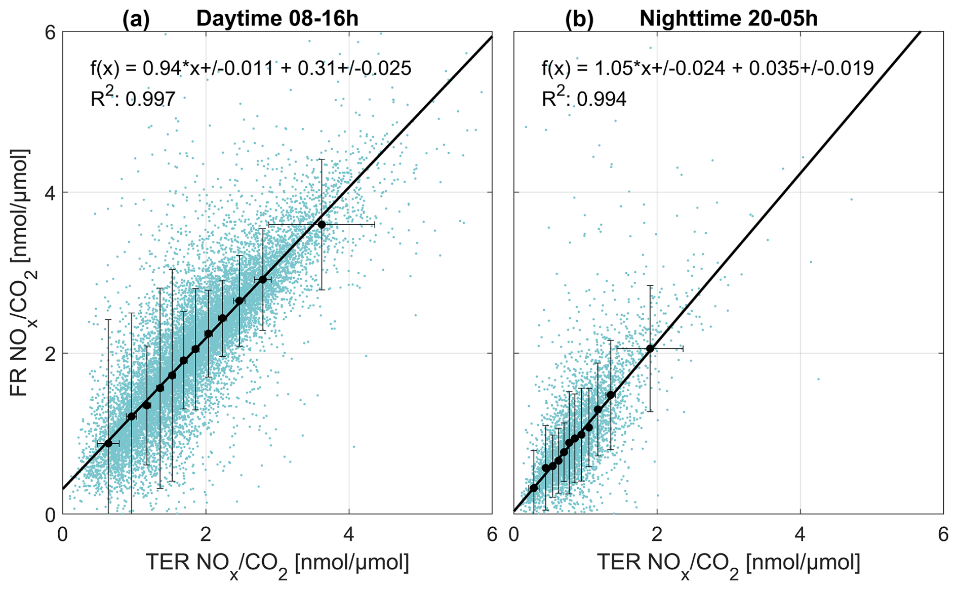
Figure 1 Comparison of TER and FRs for daytime (a) and nighttime (b). The turquoise points are QA/QC-filtered half-hourly ratios for the entire campaign. Black points (with error bars representing the standard deviation) are the medians binned into intervals with an equal number of data points per bin. The solid line is the regression line for the black points.

2.3 Dataset

The dataset spans mid-2018 to early 2022, achieving an overall data coverage of 88.9 %. Data gaps are primarily due to laboratory and instrumentation maintenance, which were minimized as much as possible. The fluxes used for calculating the flux ratios were determined following the methodology outlined by Striednig et al. (2020) and included sonic tilt correction, lag time correction, detrending, and despiking. To account for lags between instruments, resulting from residence times within the sampling tubes and potential filter contamination, corrections were applied using a widely accepted cross-covariance analysis performed at half-hourly intervals. The dataset also captures the period of the global COVID-19 pandemic, which affected Austria from March 2020 to the end of 2022, including four lockdowns by the end of 2021. The dataset was filtered according to the accepted micrometeorological criteria (Foken, 2008). We used the following quality assurance/quality control (QA/QC) criteria: a signal-to-noise ratio >3, a steady-state criterion ≤0.5, a noise RMSE ≤20 for NO_x and CO₂ fluxes, and a correlation coefficient R²≥0.5 for TER, while TER and flux ratio (FR) were calculated for 30 min averages.

3 Theory

The excess mixing ratio (Yokelson et al., 2013; Andreae and Merlet, 2001) is derived by subtracting the background of the species of interest X from its mixing ratio within a plume:

$$\begin{array}{}\text{(1)}& {\mathrm{EMR}}_X=X-X_{\mathrm{bg}},\end{array}$$

where X is the measured mixing ratio within the plume, and X_bg the background reference value measured outside the plume. The normalized enhancement ratio is then calculated by dividing the EMR of X by the EMR of a reference species Y (preferably of long atmospheric lifetime):

$$\begin{array}{}\text{(2)}& {\mathrm{NER}}_{X/Y}={\displaystyle \frac{X-X_{\mathrm{bg}}}{Y-Y_{\mathrm{bg}}}}.\end{array}$$

If the background values of X and Y are not determinable, Yokelson et al. (2013) describe the NER${}_{X/Y}$ as the slope of the regression line between species X and Y:

$$\begin{array}{}\text{(3)}& {\mathrm{NER}}_{X/Y}={\displaystyle \frac{\stackrel{\mathrm{‾}}{XY}}{{\stackrel{\mathrm{‾}}{\left(Y\right)}}^{\mathrm{2}}}},\end{array}$$

where $\stackrel{\mathrm{‾}}{XY}$ is the covariance between X and Y, and ${\stackrel{\mathrm{‾}}{\left(Y\right)}}^{\mathrm{2}}$ is the variance of Y. For single-plume studies, this approach is often sufficient to characterize the source, but in areas with superimposed and different emitters, such as those common in complex urban settings, we propose an extension to Eq. (3) by relating enhancement ratios to turbulent motions (e.g. Van der Hoven, 1957). Therefore, Eq. (3) will be adapted by applying Reynolds decomposition, which allows us to resolve the turbulent part of the spectrum (TER):

$$\begin{array}{}\text{(4)}& {\mathrm{TER}}_{X/Y}={\displaystyle \frac{\stackrel{\mathrm{‾}}{(\stackrel{\mathrm{‾}}{X}+X{}^{\prime })(\stackrel{\mathrm{‾}}{Y}+Y{}^{\prime })}}{{\stackrel{\mathrm{‾}}{(\stackrel{\mathrm{‾}}{Y}+Y{}^{\prime })}}^{\mathrm{2}}}}\stackrel{\text{Reynolds' assumptions}}{⟶}{\displaystyle \frac{\stackrel{\mathrm{‾}}{X{}^{\prime }Y{}^{\prime }}}{\stackrel{\mathrm{‾}}{(Y{}^{\prime }{)}^{\mathrm{2}}}}},\end{array}$$

where X^′ (Y^′) can be interpreted as the fluctuating parts around the mean $\stackrel{\mathrm{‾}}{X}\left(\stackrel{\mathrm{‾}}{Y}\right)$.

Fast measurements (e.g. 1–10 Hz) allow for resolving the fluctuating parts. Scales centred around the peak in the co-spectrum and into the inertial subrange can then be interpreted as a turbulent enhancement ratio (TER) and, in analogy to eddy covariance flux measurements (F(X), F(Y)), reflect an aggregated primary source emission ratio between compounds X and Y:

$$\begin{array}{}\text{(5)}& {\mathrm{FR}}_{X/Y}={\displaystyle \frac{\stackrel{\mathrm{‾}}{w{}^{\prime }X{}^{\prime }}}{w{}^{\prime }Y{}^{\prime }}},\end{array}$$

where w^′ represents fluctuations in vertical wind speed. We tested the TER calculation on typical timescales customary for eddy covariance flux observations, capturing timescales from 0.1 s to 1800 s, where the averaging filter can be adjusted based on the measurement location. We interpret the TER as the unbiased spectrally resolving enhancement ratio and the NER as a biased quantity depending on the filter scale, which subsequently defines what can be resolved. Unlike conventional NERs, which are often derived from ensemble averages (e.g. Parrish et al., 2002; Ehrnsperger and Klemm, 2021), the TER method retains high-frequency turbulent information, making it better suited for complex source separation in dynamically evolving urban environments.

4 Results

4.1 Validation of the turbulent enhancement ratio

A key issue for measuring EMRs in complex urban environments is that the difference between the background and plume enhancement is often not well defined due to the superposition of many individual plumes. This can introduce biases far away from sources. Figure 1 presents the comparison between the TER and the flux ratio (FR) of NO_x over CO₂, segregated into daytime (left panel) and nighttime (right panel) periods averaged over 30 min. We consider the flux ratio as the reference method, as it is directly related to surface emission variations. The daytime period from 08:00 to 16:00 UTC typically features a well-mixed planetary boundary layer (PBL) with pronounced turbulence so that the accuracy of eddy covariance (EC) methods is generally well accepted. Conversely, nighttime conditions often do not meet EC criteria due to reduced turbulence and a higher relative influence of horizontal advection fluxes. Therefore, the time series data have been filtered using standard QA/QC criteria as outlined in Foken (2008). Due to the urban heat island effect, we typically do not see a pronounced stratified stable urban nocturnal boundary layer in Innsbruck. In fact, most of the time, we observe unstable conditions during nighttime, which has been observed at many other urban sites (e.g. Christen and Vogt, 2004; Oke et al., 2017; Ward et al., 2022).

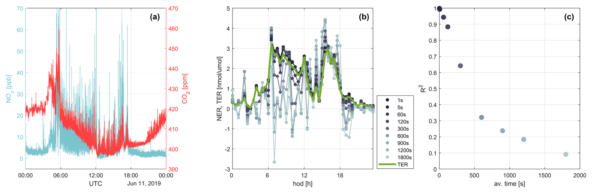
Figure 2 (a) Volume mixing ratios for NO_x (turquoise line) and CO₂ (red line) on 11 June 2019, with a sampling rate of 5 Hz. (b) The TER (green line) and the NER (grey to black lines) for different averaging intervals (1 s to 1800 s) for each half hour beginning from midnight. (c) Comparison of the coefficient of determination (R²) between TER and NER as a function of averaging time.

Both daytime and nighttime periods exhibit high linearity between the TER and FR, with R² values of 0.99, indicating a strong correlation. The regression slopes range from 0.94 during the day to 1.05 at night, reflecting a consistent relationship within the uncertainty bounds. Daytime ratios typically exhibit a broader range, with most values extending up to ∼ 4 nmol µmol⁻¹, compared to nighttime ratios, which are generally lower. This variation is caused by differences in source contributions between day and night, such as reduced traffic emissions during nighttime.

The limits of the observed ratios align well with typical NO_x $/$ CO₂ ratios reported in the literature for urban activities, supporting the validity of the measurements (e.g. the NO_x $/$ CO₂ ratio for domestic fuel derived from EMIKAT (https://www.emikat.at, last access: 28 August 2024) is 0.83 nmol µmol⁻¹, the NO_x $/$ CO₂ ratio for traffic is on the order of ${\mathrm{3.3}}_{\mathrm{2.0}}^{\mathrm{5.3}}$ nmol µmol⁻¹ $\left(X_{\min }^{\max }\right)$ (Peitzmeier et al., 2017)). Generally speaking, combustion processes from domestic fuel burning are cleaner in terms of NO_x emissions, due to lower combustion temperatures (Zeldovich mechanism) and better-controlled burning conditions; per emitted CO₂, about 3–4 times more NO_x is emitted from internal combustion engines of motor vehicles (Oland, 2002; Karl et al., 2017).

The analysis demonstrates a robust linear relationship between TER and FR across both day and night periods; it underscores the reliability of using TER as an alternative to FR in complex urban settings.

Figure 2a illustrates the volume mixing ratios of NO_x and CO₂ over the course of a single, sunny summer day (11 June 2019). The NO_x concentrations exhibit a characteristic diurnal pattern, with low levels and minimal variation during the night, followed by a marked increase in the early morning, coinciding with the rise in traffic activity. Throughout the day, strong atmospheric turbulence ensures efficient vertical transport of NO_x from the street canyon to above the urban roughness layer, resulting in the detection of numerous plumes. These plumes have durations ranging from a few seconds to fractions of a minute. The CO₂ signal displays the expected diurnal cycle, characterized by elevated levels during the night and a daytime minimum attributable to photosynthetic activity, accompanied by increased variability. Spikes in the CO₂ signal frequently correlate with those in the NO_x data, suggesting a common source. The signals of NO_x and CO₂ reflect the influence of multiple superimposed sources within a complex environment, where traditional methods for quantifying emissions are only partially effective.

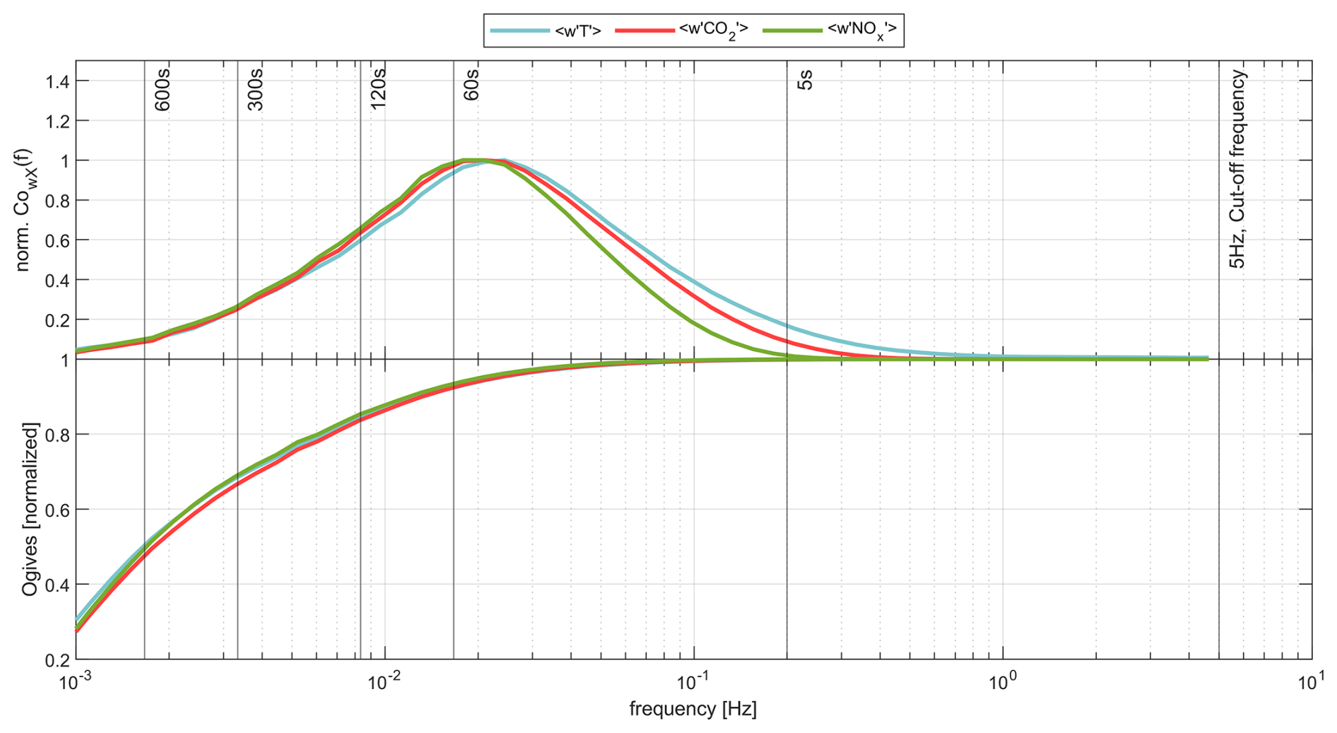
Figure 3 The upper panel shows the normalized co-spectra for sensible heat flux (blue), CO₂ flux (red), and NO_x flux (green) as a function of frequency (log scale). The lower panel shows the corresponding normalized ogives.

Figure 2b provides a more detailed comparison of TER and NER calculated for different filter timescales ranging from 1 s to 1800 s throughout the diurnal cycle. The observed pattern aligns well with the expected behaviour, displaying background levels during the nighttime and elevated values during the day, predominantly influenced by traffic emissions. During the nighttime, the agreement between different averaging periods improves as high-frequency fluctuations are suppressed, allowing larger-scale eddies to dominate, which are less impacted by low-pass filtering. Additionally, since the turbulence measurements are taken at approximately 42 m above the ground, they are more influenced by larger eddies, further improving correlation for longer averaging periods. However, when turbulence is strongly pronounced and boundary layer dynamics increase, particularly during the morning and evening, substantial variability is evident, and in some cases, the enhancement ratios may not be accurately represented. This effect becomes especially relevant during critical time periods such as rush hour, where short-term emission peaks play a crucial role in accurately characterizing emission sources. Since NER's ability to capture these variations depends on the averaging interval, excessively long sampling times could lead to an information gap, potentially underestimating peak emissions and their temporal variability. To further investigate the extent to which different averaging intervals influence the agreement between these two metrics, Fig. 2c quantifies this relationship by depicting the coefficient of determination (R²) as a function of averaging time. The results indicate a strong correlation (R²>0.9) for short averaging intervals up to 60 s, confirming that both metrics capture the turbulent dynamics effectively at these timescales. However, as the averaging period increases, the agreement deteriorates rapidly. For standard air quality monitoring stations (in Austria) that typically employ 600 s (10 min) sampling intervals, most of the turbulence spectrum is already lost, leading to a significant drop in correlation (R²<0.4). This suggests that longer averaging intervals may be insufficient to capture the influence of turbulence-driven fluctuations in urban environments, particularly during high-emission periods. The inability to resolve these rapid variations may introduce uncertainties into emission assessments and hinder the accurate representation of short-term pollution dynamics.

Figure 3 presents an analysis of the frequency-dependent behaviour of the flux co-spectra and their corresponding cumulative contributions (i.e. ogives) at the field site. The upper panel displays the normalized co-spectra of the sensible heat flux, CO₂ flux, and NO_x flux, with the sensible heat flux serving as a reference, as it is expected to be minimally affected by damping. The peak of the co-spectra typically occurs at around 60 s for the NO_x flux. The high surface roughness in the urban inertial sublayer and measurement height shift the peak of the turbulent spectrum towards longer timescales, as larger-scale eddies dominate the transport. At higher frequencies, a systematic damping effect is observed for the CO₂ and NO_x fluxes, indicative of low-pass filtering effects likely caused by instrumental response and averaging methodology. This phenomenon relaxes the stringent requirements for high-frequency sampling at this location (42 m above the ground), as turbulent transport occurs on relatively larger scales.

The lower panel of Figure 3 summarizes the corresponding ogives, which quantify the cumulative flux contributions across different frequencies. Scale-dependent analysis is a common approach in micrometeorology to separate important contributions to the co-spectrum. In this context, we interpret the TER as a spectral similarity ratio, similar to approaches used to filter data in turbulent flows (Antonia et al., 1987; Nappo, 2012). This provides further insight into the degree of flux loss associated with various averaging periods. The results demonstrate that for averaging intervals down to 60 s, the damping effect is minimal, with only a 7 % loss of the total flux. However, typical air quality observations are often conducted on timescales between 10 min and 1 h. A NER analysis in these cases would miss >50 % of the fluctuation, confirming that longer averaging intervals lead to a significant underestimation of fluxes and corresponding TER. Due to the high roughness at the current locations, observations on the order of 5 s would retain 99.9 % of the total spectrum. These findings highlight the critical role of sampling frequency relative to sampling location for accurately resolving turbulent fluxes in urban environments and emphasize the importance of maintaining sufficiently high sampling rates.

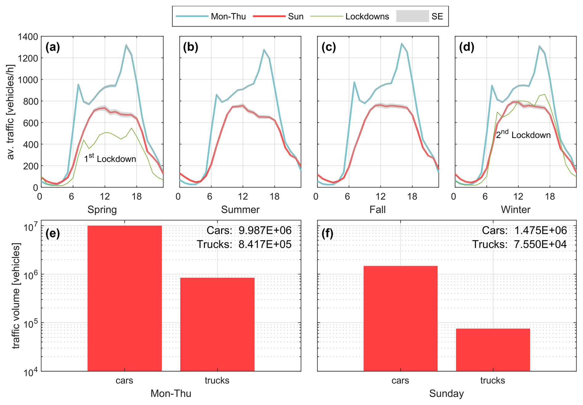
Figure 4 Seasonal traffic patterns and vehicle type distribution at the field site. Panels (a)–(d) show the average daily traffic volume, with the turquoise line representing weekdays (Mon–Thu) and the red line representing weekends (Sun). The green lines in panels (a) and (d) indicate the daily traffic patterns during the first and second lockdown, respectively. The grey shaded area represents the standard error. Panels (e) and (f) display the overall traffic volume for weekdays (e) and weekends (f), with separate bars for cars and trucks.

4.2 Traffic analysis

Traffic plays a crucial role for CO₂ and NO_x emissions in Innsbruck and, besides domestic fuel use, is the second most prominent emission source within the measurement footprint. Variations in traffic volume can significantly shift the NO_x $/$ CO₂ ratio, resulting in a greater influence of other sources. Figure 4 illustrates the traffic data collected at a monitoring station operated by the government of Tyrol, located very close to the field site and representative of the traffic activity within the flux footprint. The predominant vehicle type is passenger cars, with nearly 10 million vehicle counts during the campaign. Trucks, including heavy-duty vehicles (HDVs), light-duty vehicles (LDVs), and buses, account for 8.4 % of total traffic on weekdays and even less (5.1 %) on weekends, making passenger cars a major player at the field site.

The diurnal traffic pattern remains consistent across all seasons, characterized by a rapid increase in the morning hours. After reaching a local maximum around 07:00 UTC, traffic volumes remain relatively stable throughout the day, with a slight upward trend, peaking in the late afternoon. Nighttime traffic volumes typically hover around ${\mathrm{99}}_{\mathrm{20}}^{\mathrm{687}}$ vehicles per hour (vph), increasing to approximately ${\mathrm{936}}_{\mathrm{770}}^{\mathrm{1330}}$ vph (on average) during the day. Seasonal variations in traffic volume are minimal and do not indicate a significant change between summer and winter.

The weekday/weekend effect typically results in a reduction of around 28.5 % during weekends, which is primarily driven by changes in commuter traffic. While weekend nighttime traffic is slightly elevated due to leisure activities, daytime values are significantly lower in line with reduced weekend activities. Notably, the rush hour peaks are absent on weekends; after reaching a plateau, there is little variability until traffic levels approach the weekly average again towards the end of the day, when traffic activity drops off sharply.

The COVID-19 pandemic and the associated lockdowns in Austria had a direct impact on traffic volumes due to mobility restrictions, though the effects varied across different lockdowns. The first, more stringent lockdown in March/April 2020, which included a total curfew, led to a nearly −55 % reduction in traffic activity. In contrast, subsequent lockdowns, which were more relaxed, resulted in a more modest traffic reduction and were comparable to the weekend traffic load and patterns. Interestingly, even during the lockdown periods, a small rush hour peak was still visible in the data, indicating some level of consistent traffic activity.

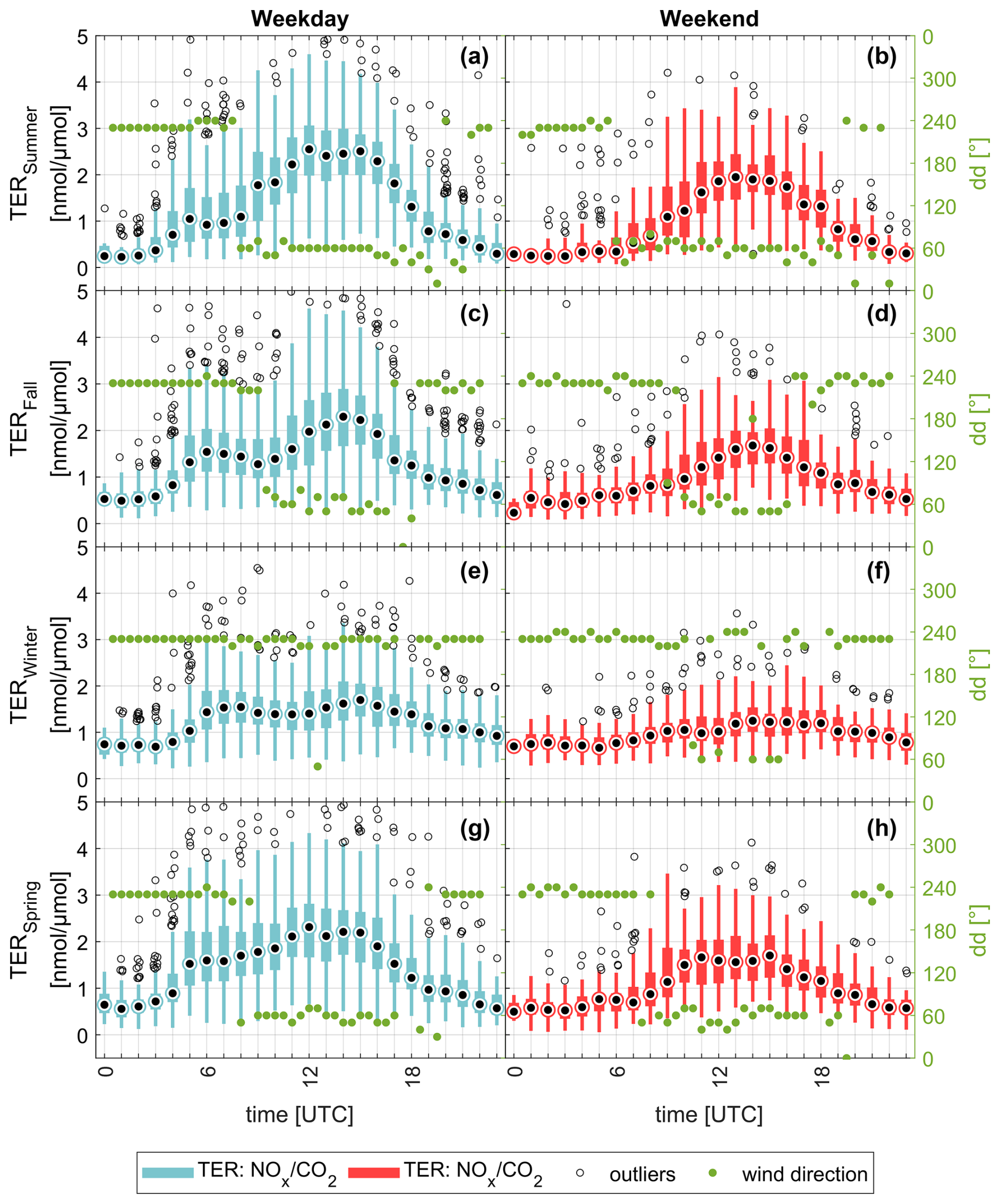
Figure 5 Box plots of the hourly TER during weekdays (Monday to Thursday, left) and weekends (Sunday, right) throughout the seasons. Black dots represent median values, circles indicate outliers, and the bars the interquartile range and the overall distribution. The green points denote the predominant wind sectors for each time interval.

4.3 Case studies

4.3.1 Weekly and seasonal trends

Based on these findings, we apply the TER analysis to a long-term dataset of the same period as used in the previous traffic data comparison. Figure 5 provides a detailed analysis of the TER of NO_x over CO₂ across various seasons and times of the day, highlighting the significant influence of both diurnal and seasonal variations. The figure showing the TER analysis between weekdays (Monday to Thursday) and weekends (Sunday). Across all seasons, the lowest TER values are observed during the nighttime, reflecting ratios typically associated with domestic fuel use. In contrast, the highest TER values occur in the early afternoon, corresponding to ratios indicative of traffic-related emissions.

The sharp increase in TER during the morning hours is closely aligned with increasing traffic, a major contributor to NO_x and CO₂ emissions, and high TER values (2–5 nmol µmol⁻¹). Weekend TERs are generally lower compared to weekdays, which can be attributed to the absence or delay of morning rush hour traffic and an overall reduction in traffic load.

The variability in TER across different seasons reflects changes in both anthropogenic and meteorological factors. The primary driver is the shift in domestic fuel use, particularly the increased use of heating systems during the winter, which significantly impacts emissions. In contrast, during the intermediate seasons of spring and autumn, atmospheric conditions, such as warmer weather periods, play a crucial role in modulating domestic fuel consumption. The impact of vegetation on CO₂ fluxes at the field site is negligible (Lamprecht et al., 2021). Another contributing factor is the seasonal variability of the measurement footprint, where even minor shifts can result in a greater or lesser influence of traffic-related emissions. The diurnal cycle of TER consistently shows a significant increase when wind patterns shift from down-valley winds (typically at night) to up-valley winds during the day, due to the differing land use characteristics within the diurnal footprint (see Fig. S2). During synoptic weather conditions in the winter, west winds prevail almost throughout the entire day on average, resulting in signals originating from a region associated with low NO_x $/$ CO₂ ratios (E, F). Figure S4 further supports this finding through a wind-sector-dependent analysis of TER, showing that on average, TER is 38 % lower in the west sector compared to the east sector.

Figure 6 provides a detailed analysis of the average NO_x and CO₂ fluxes as a function of the daily mean temperature. Panel (a) shows that CO₂ fluxes exhibit a distinct negative correlation (dCO₂/d_T $=-\mathrm{0.49}$ µmol K⁻¹) at temperatures below 12 °C, consistent with Ward et al. (2022). Above this threshold, the CO₂ flux stabilizes (dCO₂/dT $=+\mathrm{0.02}$ µmol K⁻¹), indicating that emissions remain relatively constant at higher temperatures. This shift aligns well with the Austrian norm ÖNORM H 7500-3, locally known as the Heizgrenze (heating threshold), which regulates heating system activation when outdoor temperatures drop below 12 °C.

The strong temperature dependence of CO₂ fluxes can be directly attributed to methane consumption from gas heating systems, which dominate the heating sector in the flux footprint. As outlined in Stichaner et al. (2024), methane consumption follows a pronounced temperature dependency below the heating threshold, a pattern that is mirrored by the CO₂ fluxes analysed here. Furthermore, photosynthetic activity plays only a minor role in this footprint (see Fig. S2b) and does not significantly affect the site as a CO₂ source. This further supports the conclusion that heating-related emissions, rather than biogenic processes, drive the observed temperature dependence of CO₂ fluxes.

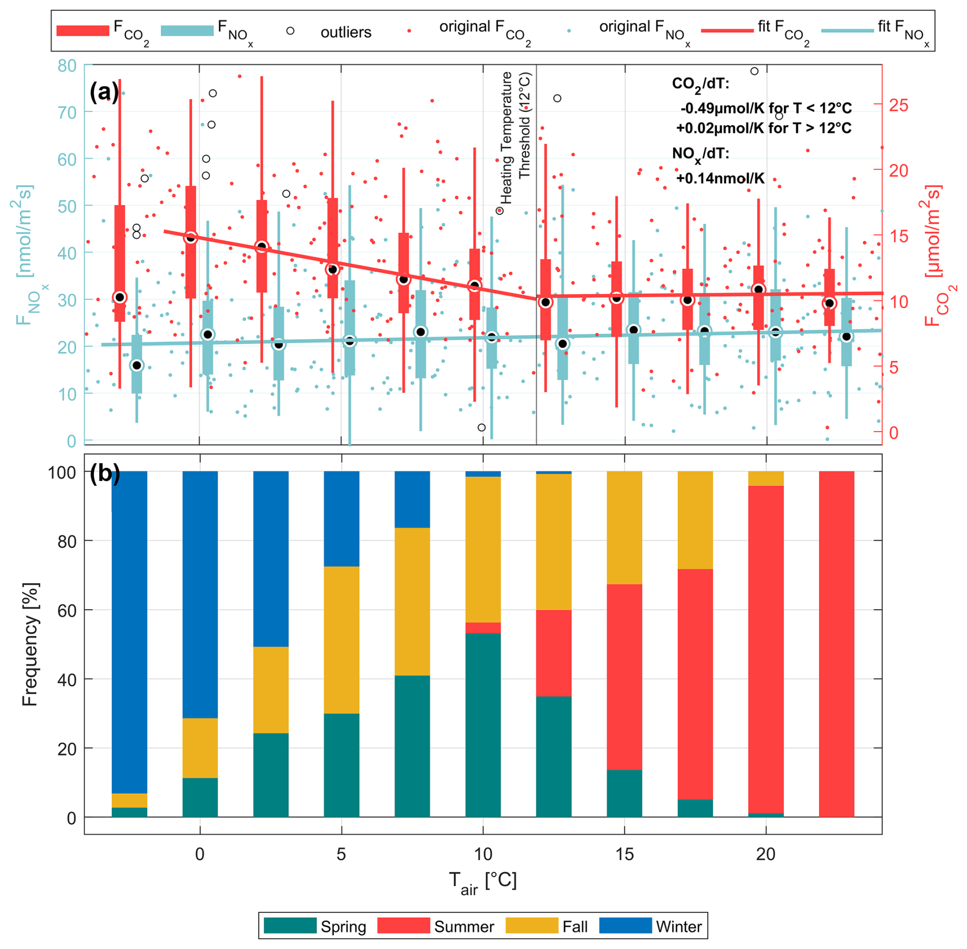
Figure 6 (a) Temperature dependency for CO₂ (red dots) and NO_x (turquoise dots) fluxes across daily mean temperatures ranging from −5.0 to 25.0 °C. The box plot is split into 2.5 K intervals, where the black dots indicate the median and the other box plot elements illustrate the interquartile range and whiskers. Black circles represent outliers. The linear fit for NO_x fluxes is calculated across the entire temperature range, while for CO₂ fluxes, it is separated into two regions (T₁<12 °C, T₂>12 °C) excluding the values for $<-\mathrm{2.5}$ °C. The black vertical line at 12 °C marks the heating temperature threshold for Austria. (b) The frequency of occurrence of the binned daily mean temperatures, grouped by season.

In contrast, the NO_x flux demonstrates a different pattern. It shows a very moderate positive temperature dependence (dNO_x/dT $=+\mathrm{0.14}$ nmol K⁻¹) that is relatively constant across the entire range of temperatures examined. This suggests that NO_x emissions, which are largely influenced by traffic, do not vary significantly with temperature changes. The interplay of these two trends is reflected in the turbulent enhancement ratio, which decreases at lower temperatures. This decrease can be attributed to the increase in CO₂ sources, which become more prominent as temperatures drop, thereby altering the ratio between NO_x and CO₂.

Panel (b) highlights the frequency of occurrence of daily mean temperatures, binned in 2.5 K sectors, across different seasons. This comparison reveals a clear trend towards higher CO₂ fluxes during colder seasons. The analysis suggests that the colder months are characterized by increased domestic heating, which significantly contributes to CO₂ emissions.

4.3.2 Lockdown vs. non-lockdown

In March 2020, the COVID-19 pandemic reached Austria, with Tyrol becoming a hotspot during the first wave. A strict lockdown, including a state-wide quarantine, was implemented from 16 March to 13 April, with a full easing of measures by mid-May. According to an analysis of emission changes by Lamprecht et al. (2021) during this period, NO_x and CO₂ emissions decreased to different levels, which should also be evident in relative changes of the TER. Such significant shifts from road to non-road sources have also been observed in London during pandemic restrictions (Cliff et al., 2023). For the analysis shown in Fig. 7, the first lockdown period was compared with the corresponding non-lockdown period in 2019. Panels (a) and (b) present the associated TERs for weekdays (a) and weekends (b). Comparing the relative changes between the TER during the first lockdown (in March 2020) and the reference period (March 2019) shows significant reductions of $-{\mathrm{32.2}}_{-\mathrm{14.9}}^{-\mathrm{49.2}}$ % on weekdays and $-{\mathrm{55.1}}_{-\mathrm{22.9}}^{-\mathrm{76.1}}$ % on weekends, with the most pronounced decrease occurring during rush hours, although the overall diurnal cycle remains unchanged. The large variability in reduction rates between weekdays and weekends can be attributed to the small number of Sundays (4) during this intense operational period (IOP), coinciding with a transitional phase in Austria from cold to warmer weather. Synoptic variability during this time had a significant influence on the local footprint and emission changes, which introduces some limitations into the interpretation.

Compared to the approximately 55 % reduction in weekday traffic during the lockdown, the decrease in TER is less pronounced. This is due to the complex interplay of various emission ratios that determine the TER. In addition to the reduction in traffic, there was also a decrease in emissions from domestic heating. This is evident from the diurnal temperature profile shown in panel (c). In 2020, daytime maximum temperatures (08:00–16:00 UTC) were on average 2.4 ± 0.3 °C higher (with a maximum of 4.3 °C) than in 2019, leading to a 16.7 % reduction in heating days and consequently reduced energy consumption for heating systems. According to the Google Environmental Insights Explorer (https://insights.sustainability.google/, last access: 26 August 2024), energy production for heating and hot water in the region is derived from electric power (37.5 %), gas (31.3 %), and oil (31.3 %), with the latter two being significant sources of NO_x and CO₂ emissions in the footprint. As emissions from sources with smaller ratios decrease, the relative impact of other emission ratios becomes more pronounced, resulting in a TER that remains higher than the traffic reduction alone would suggest. Overall, the observed TER changes with and without a lockdown are generally consistent with the modelled emission changes based on direct flux observations (Lamprecht et al., 2021) with changes between −59 % for NO_x and −38 % for CO₂ fluxes.

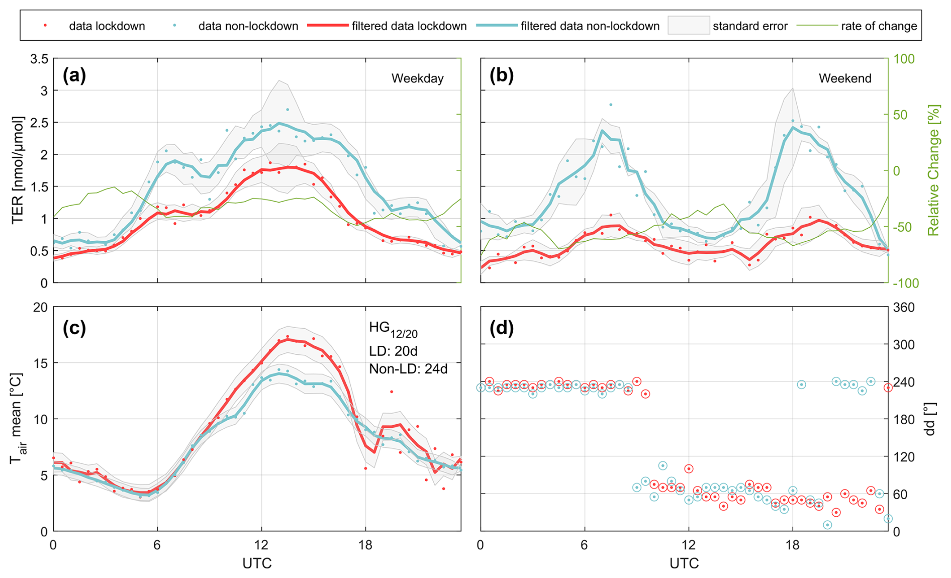
Figure 7 Comparison of the TER (a, b), temperature (c), and wind direction (d) during the first COVID-19 lockdown in 2020 with a non-lockdown period in 2019. The points in (a) and (b) represent the original TER values for the lockdown (red) and non-lockdown (turquoise) periods for weekdays and weekends, respectively. The corresponding solid lines represent a 3-point moving average, with the grey shaded area indicating the standard error. The relative change between the TER during lockdown and non-lockdown is shown by a solid green line. Panel (c) presents the diurnal temperature profiles, along with the numbers of heating days for the lockdown (LD) and non-lockdown (Non-LD) periods. Panel (d) illustrates the predominant wind directions in 10° intervals for both IOPs.

Figure 7d illustrates the dominant half-hourly wind directions during the IOPs, providing insights into potential differences in the turbulent footprint of the measurements. Both IOPs exhibit relatively similar wind regimes with minimal variability, except the time between 18:00 UTC and midnight. During this period, the wind direction during the lockdown phase shifts back to 240° (down-valley wind), whereas in 2019, the wind remains predominantly within the 0–60° sector. Nevertheless, the overall comparability between the two periods is strong, as the prevailing wind regimes ensure that the same source areas were consistently captured during the key daytime hours (08:00–16:00 UTC). To further assess potential differences in meteorological conditions between the two periods, we also analysed stability conditions (represented by the Monin–Obukhov length) and cross-wind patterns (Fig. S3). The results indicate that no significant differences were found between the lockdown and non-lockdown periods. This further reinforces the robustness of the observed pollutant variations, confirming that changes in air quality were primarily driven by emission reductions rather than shifts in meteorological conditions.

5 Discussion and summary

Here, we demonstrate that time-resolved observations of air pollutants, which capture most of the variance in the turbulent flow, can be used to determine local enhancement ratios of different air pollutants. Turbulent enhancement ratios (TERs) are in excellent agreement with flux ratios derived from eddy covariance observations of NO_x and CO₂ in the city of Innsbruck. The advantage of the turbulent enhancement method is that, in principle, no additional instrumentation beyond the tracer observations is required. This makes the approach highly flexible and applicable to a variety of urban and industrial settings. The analysis presented here can be used in combination with a growing number of advanced measurement technologies, such as spectroscopic and mass spectrometric techniques, which are increasingly capable of capturing multiple species at high time resolution. The interpretation of turbulent enhancements will vary by location but can be experimentally determined by the analysis of spectra and co-spectra. Unlike traditional flux measurements, these types of observations do not necessarily require extensive data pre-treatment or assumptions that are often used for eddy covariance observations. The relevance of experimentally resolving TER becomes particularly strong when the measurement site is close to an emission source, as turbulent mixing plays a dominant role in determining enhancement ratios. Morning and evening hours, when the planetary boundary layer (PBL) undergoes strong transitions, are particularly critical in this context, as shifting vertical mixing conditions directly impact the observed ratios. Here we observed biases of >50 % using NER on scale averages >10 min. At these times, turbulence-driven variations in enhancement ratios are more pronounced, and high-frequency sampling is necessary to resolve these fluctuations accurately. In contrast, when turbulence largely decreases and the flux footprint increases, such as during stable nighttime conditions or under weak turbulence, scale average NER values up to 1800 s approach TER values as the source contributions are more non-local. Under such conditions, high-frequency sampling becomes less critical, and NERs derived from slower sampling rates agree more closely with TER, as seen for nighttime data. For many air quality monitoring stations across Europe, where time resolutions of 10 min (600 s) are standard, the ability to determine enhancement ratios is largely restricted to periods of strong agreement between NER and TER, such as during nighttime or under stable meteorological conditions. However, during the most relevant time periods for urban emissions, such as rush hour or periods of strong boundary layer evolution, these longer averaging intervals introduce significant biases by smoothing out short-term variations in the data. Our analysis highlights that a simple increase in sampling frequency would greatly improve the ability to study emission sources in urban environments. Specifically, we show that for sampling intervals below 60 s, only 7 % of the total flux spectrum is lost, whereas at 600 s, 50 % of the turbulence spectrum is missing, leading to substantial underestimation of emissions and their temporal variability.

In Innsbruck, long-term analysis of the TER shows that the NO_x $/$ CO₂ enhancement ratio can be explained by the superposition of two main sources: traffic and energy usage for heating and warm-water generation. We are able to describe the variation of the turbulent enhancement ratio of NO_x $/$ CO₂ based on the superposition of traffic activity and temperature-driven activity in the urban energy sector (including residential, commercial, and public emissions). In summer, the daytime TER lies close to the expected ratio from traffic emissions (e.g. 2–5.3 nmol µmol⁻¹; Peitzmeier et al., 2017). In winter, a higher fraction from heating in the urban energy sectors is evident and reduces the ratio. NO_x emissions in Innsbruck are predominantly associated with traffic (e.g. >90 %; e.g. Lamprecht et al., 2021). In contrast, CO₂ emissions have a sizeable contribution from traffic and the urban energy sector. The reduction of the NO_x $/$ CO₂ ratio is therefore primarily driven by changes in CO₂ emissions throughout the season (i.e. higher emissions in winter). This explains the variation of the TER during weekends, weekday days, and different seasons and hard mobility restrictions during the COVID-19 pandemic.