A large-eddy simulation exploration of the assumptions used in retrieving entrainment from a mixing diagram approach with ground-based remote sensors

Entrainment is a crucial component of the atmospheric boundary layer (BL) moisture and heat budget. While usually thought of as only entrainment flux, entrainment within the mixed layer budget equation is really composed of two terms: the flux of a property across the boundary separating the BL from the free troposphere and the change in the concentration of a property as the depth of the BL changes. In a recent study, Wakefield et al. (2023) used ground-based remote-sensing observations to estimate entrainment flux as the residual of a mixing diagram framework that was applied to the daytime convective boundary layer. This present work uses large-eddy simulation (LES) to examine how well this residual assumption for entrainment fluxes alone compares to the actual sum of those two entrainment terms derived from spatial averages of the LES output. We highlight the importance of the second entrainment term in closing the mixed layer budget and show that the residual assumption does not represent entrainment flux only but rather a total entrainment term when the boundary layer depth is changing.

1 Introduction

The atmospheric boundary layer (BL) is the section of the atmosphere that interacts directly with the surface and is responsible for the majority of our weather. Temperature and moisture changes within the BL can impact cloud formation (Ek and Mahrt, 1994; Findell and Eltahir, 2003; Ek and Holtslag, 2004), heat waves and droughts (Miralles et al., 2014, 2019; Schumacher et al., 2019; Benson and Dirmeyer, 2021), and reintensification of tropical cyclones over land (Emanuel et al., 2008; Arndt et al., 2010; Andersen et al., 2013; Andersen and Shepherd, 2013; Wakefield et al., 2021). Therefore, more accurate representations of the evolution of the heat and moisture budgets in the BL is crucial for improving climate models, improving weather models, and ultimately forecasting extreme weather earlier.

At the top of a BL, free tropospheric air is incorporated down into the turbulent mixed layer through entrainment (Stull and Eloranta, 1984). van Heerwaarden et al. (2009) found that the entrainment of heat at the top of the BL directly increases the depth of the BL, and dry-air entrainment enhances surface evaporation, which impacts cloud formation, exposing a need for entrainment to be accurately handled in models. While an important feature, entrainment is difficult to capture through observations due to its small scales of motion compared to the convective mixing within the BL (Cooper and Eichinger, 1994; Nelson et al., 1989; Crum et al., 1987; Angevine et al., 1998), its position at the top of the BL – making it more difficult to measure with ground-based observations (Vilà-Guerau de Arellano, 2004), and the difficulty in computing horizontal averages due to instrument spacing or differing terrain (Driedonks, 1982). Determining a more robust way to estimate entrainment fluxes from ground-based observations would lead to better understanding of the changes in temperature and moisture in the mixed layer.

One method for estimating entrainment was shown in Wakefield et al. (2023) (hereafter W23), using a mixing diagram framework inspired by Betts (1992). Betts developed the mixing diagram method for analyzing aircraft data in order to study the evolution of the daytime mixed layer, using vector representations of heat and moisture budgets. This method was later applied to evaluate land–atmosphere couplings by Santanello et al. (2009). In a mixing diagram, the evolution of the heat and moisture budgets is plotted on the same figure as the vector components that make up that evolution, offering a visual representation of the contributions of various forcings to the changes within the mixed layer. Betts (1992) defined the mixed layer budget for an atmospheric property ϕ as

$$\begin{array}{}\text{(1)}& \begin{array}{rl}{\displaystyle \frac{\partial \stackrel{\mathrm{‾}}{\mathit{\varphi }}}{\partial t}}& ={\left.{\displaystyle \frac{\partial {\stackrel{\mathrm{‾}}{\mathit{\varphi }}}_{\mathrm{ml}}}{\partial t}}\right|}_{\mathrm{LS}}+{\left.{\displaystyle \frac{\stackrel{\mathrm{‾}}{w^{\prime }{\mathit{\varphi }}^{\prime }}}{z_i}}\right|}_{\mathrm{Sfc}}-{\left.{\displaystyle \frac{\stackrel{\mathrm{‾}}{w^{\prime }{\mathit{\varphi }}^{\prime }}}{z_i}}\right|}_{\mathrm{top}}\\ & +\left({\displaystyle \frac{\partial z_i}{\partial t}}-\stackrel{\mathrm{‾}}{w_i}\right){\displaystyle \frac{\left({\stackrel{\mathrm{‾}}{\mathit{\varphi }}}_{\mathrm{top}}-\langle \stackrel{\mathrm{‾}}{\mathit{\varphi }}\rangle \right)}{z_i}},\end{array}\end{array}$$

where overbars indicate horizontal averaging and angle brackets indicate averaging over the depth of the BL. The terms in this equation are the following:

•  

  $\frac{\partial \stackrel{\mathrm{‾}}{\mathit{\varphi }}}{\partial t}$ is the total change of the atmospheric property in the mixed layer over time;

•  

  ${\left.\frac{\partial {\stackrel{\mathrm{‾}}{\mathit{\varphi }}}_{\mathrm{ml}}}{\partial t}\right|}_{\mathrm{LS}}$ is the average large-scale forcing across the BL (usually the advection term but also radiative heating);

•  

  ${\left.\frac{\stackrel{\mathrm{‾}}{w^{\prime }{\mathit{\varphi }}^{\prime }}}{z_i}\right|}_{\mathrm{Sfc}}$ is the atmospheric property flux at the surface over time;

•  

  $-{\left.\frac{\stackrel{\mathrm{‾}}{w^{\prime }{\mathit{\varphi }}^{\prime }}}{z_i}\right|}_{\mathrm{top}}+\left(\frac{\partial z_i}{\partial t}-\stackrel{\mathrm{‾}}{w_i}\right)\frac{\left({\stackrel{\mathrm{‾}}{\mathit{\varphi }}}_{\mathrm{top}}-\stackrel{\mathrm{‾}}{\mathit{\varphi }}\right)}{z_i}$ is the total entrainment.

Within the total entrainment term, there is the entrainment flux (ENT1) term ${\left.\frac{\stackrel{\mathrm{‾}}{w^{\prime }{\mathit{\varphi }}^{\prime }}}{z_i}\right|}_{\mathrm{top}}$ and a second term that considers the difference between the magnitude of a property within the mixed layer and at the top of the BL $\left(\frac{\partial z_i}{\partial t}-\stackrel{\mathrm{‾}}{w_i}\right)\frac{\left({\stackrel{\mathrm{‾}}{\mathit{\varphi }}}_{\mathrm{top}}-{\stackrel{\mathrm{‾}}{\mathit{\varphi }}}_{\mathrm{ml}}\right)}{z_i}$, which we refer to as entrainment 2 (ENT2). ENT2 depends on the change in boundary layer depth over time ($\frac{\partial z_i}{\partial t}$), the subsidence ($\stackrel{\mathrm{‾}}{w_i}$), and the difference between the mean value of a property at the top of the BL and the mean value within the mixed layer (${\stackrel{\mathrm{‾}}{\mathit{\varphi }}}_{\mathrm{top}}-\stackrel{\mathrm{‾}}{\mathit{\varphi }}$). ENT1 is the flux of a property entering the boundary layer from the free troposphere above, while ENT2 accounts for the change in concentration of a property with a change in BL depth over time.

W23 showed that if the total evolution, surface fluxes, and average large-scale forcing are known, entrainment fluxes can be estimated as the residual or closure term. In that study, the thermodynamic profiles were retrieved using the TROPoe retrieval algorithm (Turner and Löhnert, 2014; Turner and Blumberg, 2019) from radiance observations made by the Atmospheric Emitted Radiance Interferometer (AERI; Knuteson et al., 2004) at the central facility of the Atmospheric Radiation Measurement (ARM) Southern Great Plains (SGP) site (Sisterson et al., 2016). To avoid the surface layer and entrainment zone, W23 computed the mean of the mixed layer properties only from 0.1z_i−0.5z_i, where z_i is the depth of the BL determined from the TROPoe retrievals using a parcel method. Surface fluxes came from a combination of surface flux measurements from the Eddy Correlation Flux Measurement (ECOR) system and the Energy Balance Bowen Ratio (EBBR) system (Cook and Sullivan, 2025). Advection was quantified with observations from an array of Doppler lidar and AERI instruments at the ARM SGP site using the method outlined in Wagner et al. (2022). Radiative heating was computed from TROPoe thermodynamic profiles using the rapid radiative transfer model (RRTM; Mlawer et al., 1997). W23 demonstrated that this approach to estimate entrainment agreed both with an observationally derived water vapor entrainment flux derived from multiple ground-based lidars and with large-eddy simulation (LES) output. However, entrainment (as described above) is really composed of two terms: the flux of a property across the boundary separating the BL from the free troposphere (ENT1) and the change in the concentration of a property as the depth of the BL changes (ENT2).

In a steady-state BL, the depth is not changing, the ENT2 term is zero, and the residual can be used to estimate the entrainment fluxes (ENT1). However, during the morning hours, the depth of the BL is usually changing relatively rapidly, and thus ENT2 can no longer be assumed to be negligible. The current study aims to show that the residual assumption agrees well with the sum of the two entrainment terms (ENT1 + ENT2) and highlight the importance of interpreting the residual of a mixing diagram (MD) as this total entrainment rather than entrainment fluxes (ENT1) alone.

Section 2 describes the methods used in this study. Section 3 presents the results of whether the residual assumption for deriving entrainment is valid, a comparison of different definitions of the mixed layer for calculating ENT2, and variability across different dates and boundary layer depth definitions. Section 4 offers a discussion of the results. Section 5 highlights conclusions and presents opportunities for future work on this topic.

2 Methods

In this study, we apply a mixing diagram framework to the morning and afternoon BL and assess its closure and stochasticity. To do this, we apply this method to large-eddy simulation output from single columns and from the entire horizontally averaged (slab) output, which serves as the truth in this study. We also investigate how computing the mean temperature and humidity only over the lower part of the mixed layer compares to when the entire mixed layer is used when computing the mean. Most of the analysis in this study focuses on 8 August 2017 case used by W23, which was synoptically quiescent and a part of the Land Atmosphere Feedback Experiment (LAFE; Wulfmeyer et al., 2018) that focused on land–atmosphere interactions. At the end of this study, results are considered for four additional dates during LAFE; i.e., 7, 14, 17, and 29 August 2017. The full analysis period is the time from just after the morning transition to just before the evening transition (08:00–17:00 CDT). This time period is split into morning hours (08:00–12:00 CDT) and afternoon hours (12:00–17:00 CDT), where the boundary layer depth is changing with time more rapidly during the morning hours than the afternoon hours.

2.1 Mixing diagrams

In a mixing diagram (MD), the total evolution of the latent and sensible heats over a specified time period is plotted, and the components (large-scale advection and radiative tendencies, surface fluxes, and entrainment) are plotted as vectors on the same figure, allowing us to visualize the contributions of all of the forcings to that diurnal evolution of sensible and latent heat. MDs are typically only used when the BL is quasi-stationary; however, this is very limiting as the BL is often changing over time. For applying a MD framework, the BL is considered well mixed during time periods where the BL is steadily growing or decaying rather than rapidly growing and decaying as it does during morning and evening transition periods. When the sum of the components (i.e., on the right-hand side of Eq. 1) equals the overall evolution in mean temperature and moisture within the well-mixed BL (i.e., the left-hand side of Eq. 1), there is closure. We define “closure” as the length of the vector distance between the total evolution and the sum of the components, as can be seen by the red arrow in Fig. 1. We can evaluate closure as the distance to close the sensible and latent heats individually or as a total vector value.

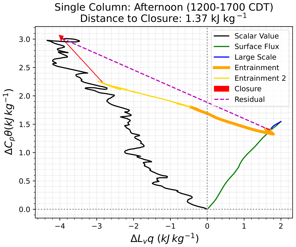
Figure 1 Mixing diagram showing the total evolution of the sensible and latent heats (black) along with the contributions to that evolution (surface fluxes in green, large-scale forcing in blue, entrainment 1 in orange, and entrainment 2 in gold), as derived from LES output where ENT1 and ENT2 are directly computed. The closure is the distance between the total evolution and the sum of the components (red arrow) and could be considered an error term in the total entrainment if it was computed as a residual (magenta).

The mixed layer budget (Eq. 1) requires that the depth of the mixed layer (i.e., the depth of the BL, also denoted z_i) be well defined and continuous. For this work, we compare three different definitions for the BL depth, which are shown in Fig. 2: the level of neutral buoyancy of a surface-based parcel of air (green), the level where the maximum humidity variance occurs (orange), and the level where the minimum potential temperature flux exists (blue).

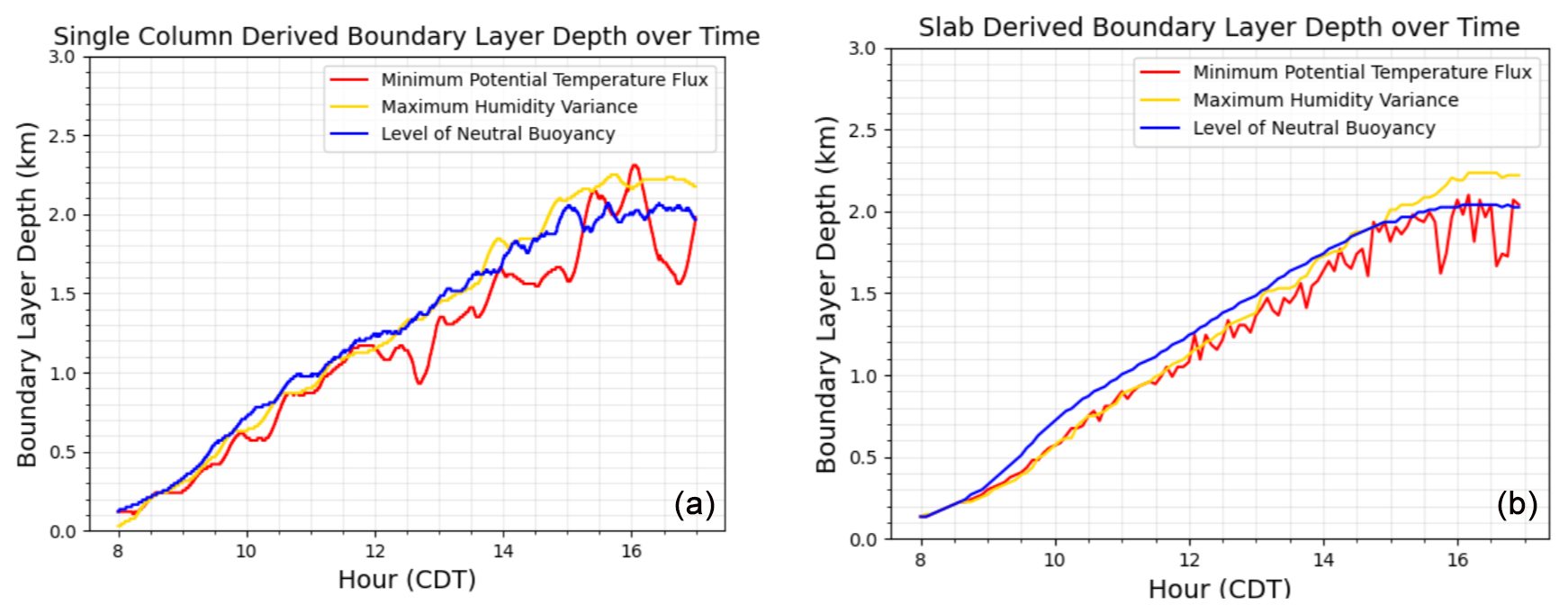
Figure 2 Comparison of three different BL depth definitions over the entire analysis period (08:00–17:00 CDT): the level of neutral buoyancy of a surface-based parcel of air (green), the maximum humidity variance (orange), and the minimum potential temperature flux (blue). Definitions are derived from the 30 min temporal average of the instantaneous values of the single column (a) and from the 5 min slab averages of values (b).

2.2 Large-eddy simulations

This work uses single-column output from large-eddy simulations to act as a proxy for ground-based observations. Informed by DALES (Heus et al., 2010), UCLA-LES (Stevens et al., 2005), and PALM (Maronga et al., 2015), MicroHH (van Heerwaarden et al., 2017) is a high-resolution computational fluid dynamics simulation that supports both direct numerical simulations and large-eddy simulations (LES). MicroHH uses the anelastic approximation to solve the governing equations of conservation of mass, momentum, and energy (Bannon et al., 2006). LES is useful in testing observational hypotheses since it gives relevant variables in all spatial and temporal dimensions. The data are internally consistent, and budgets that are calculated from these data must close by definition, down to the discretization error. In this study, we will use slab-averaged values (i.e., averaged values over the entire LES domain at each vertical level) as the “truth”. We want to investigate how real observations, which are making time series observations at a single point, are able to represent spatial statistics; thus, we are comparing statistics computed at a single location within the LES domain against the slab averages.

Model configuration

MicroHH uses a second-order central differencing spatial discretization scheme and a fourth-order Runge–Kutta time integration method on an Arakawa C grid. Potential temperature (Θ) and water vapor mixing ratio (q) are carried as thermodynamic variables and are conserved for adiabatic processes. The simulation uses ARM's constrained variational analysis (VARANAL) for initial and boundary conditions (Xie, 2004). VARANAL provides values for surface fluxes, large-scale advective and radiative tendencies that are applied in a spatially homogeneous way, averaged over the entire ARM SGP domain. We set a 15 m vertical grid spacing from the surface to 4200 m and 10 m horizontal grid spacing over a 6400 m domain size with periodic boundary conditions. To accurately simulate the diurnal evolution of the atmospheric boundary layer, we chose a 6400 m domain size that is several times the BL depth but still able to resolve turbulence producing scales of the BL (Fedorovich et al., 2004). The LES is run for 7, 8, 14, 17, and 29 August 2017 starting at 03:00 UTC and run for 20 h. Output from 64 individual columns that are equidistantly placed across the domain with 10 s temporal resolution acts as profile observations.

2.3 Entrainment fluxes

Since the LES columns do not yield both temperature and water vapor entrainment fluxes directly, we use the following for calculating ENT1 from the single-column output:

$$\begin{array}{}\text{(2)}& \begin{array}{rl}\stackrel{\mathrm{‾}}{w^{\prime }{\mathit{\varphi }}^{\prime }}\left(t\right)& =\sum _{t-t_{\mathrm{1}/\mathrm{2}}}^{t+t_{\mathrm{1}/\mathrm{2}}}{\displaystyle \frac{\mathrm{1}}{N}}\left({\mathit{\varphi }}_{z=zi\left(t\right)}-{\mathit{\varphi }}_{\mathrm{avg},z=zi\left(t\right)}\right)\\ & \times \left(w_{z=zi\left(t\right)}-w_{\mathrm{avg},z=zi\left(t\right)}\right),\end{array}\end{array}$$

where ϕ_z and ϕ_avg,z represent a general property and the mean of that general property, while w_z and w_avg,z are the vertical velocity and the mean of the vertical velocity all at the top of the boundary layer. In this calculation, we estimate ENT1 using a time series of data from a single column within the LES domain, choosing an analysis period averaged over a 1 h period centered on each 30 min to reduce the sampling uncertainty (Lenschow et al., 1994). Previous studies typically performed the time series analysis along a constant height grid where z_i was in the center of the temporal analysis window. Instead of taking the running average of a property at a constant height, we normalize the property by the BL depth first. This means that, while taking the running average of the property, the change in BL depth is already being considered. This method is outlined in more detail in Rosenberger et al. (2024).

3 Results

3.1 Residual assumption

Figures 4 and 5 compare mixing diagrams for 8 August 2017 derived from three different BL depth definitions: the level of neutral buoyancy of a surface-based parcel of air (left), the maximum humidity variance (middle), and the minimum potential temperature flux (right), for the slab output (top row) and the single-column output (bottom row). During the morning time (08:00–12:00 CDT) shown in Fig. 4, the magnitude of the total entrainment (ENT1 + ENT2) due to latent heat is approximately 8.5 kJ kg⁻¹, and for sensible heat it is 2.5 kJ kg⁻¹ regardless of the boundary layer depth definition used. There are, however, differences in the relative magnitudes of the ENT1 and ENT2 terms depending on the boundary layer depth definition. ENT1 is approximately 30 %, 50 %, and 60 % of the total entrainment (i.e., ENT1 + ENT2) when the level of neutral buoyancy, the minimum potential temperature flux, and the maximum humidity variance are used to define the top of the BL (i.e., z_i), respectively. To see the relationship with BL depth definition more clearly, Fig. 6 shows the ratio of the slab-derived ENT1 to ENT1 + ENT2 for five different dates considered and for the three boundary layer depth definitions for the morning (left) and afternoon (right). Here, we see the relative contributions to ENT1 versus the total entrainment varies greatly with boundary layer depth definition. The entrainment zone is a layer of intermittent turbulence between the mixed layer and free troposphere where the potential temperature gradient is strongest and where the buoyancy flux is negative (Fig. 3; see Stull, 1988). The variation in ENT1 and ENT2 magnitudes tells us that the higher in the entrainment zone z_i is defined, the stronger the influence of ENT2 is.

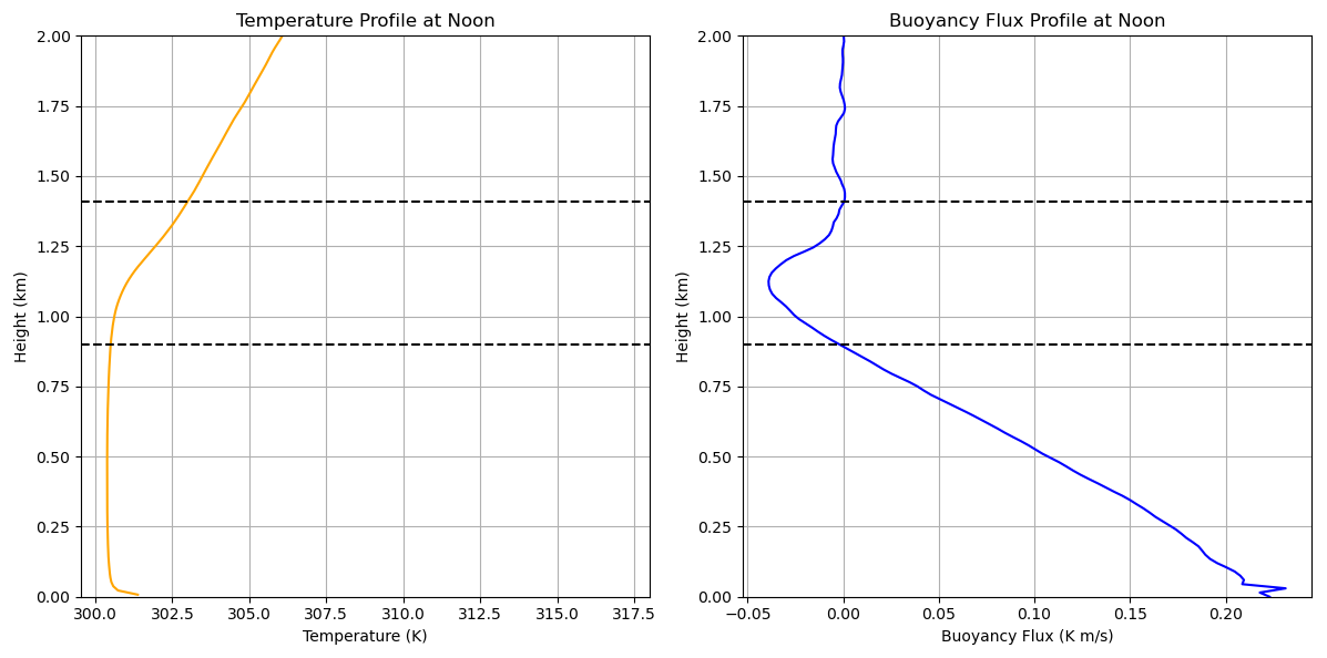
Figure 3 The potential temperature and buoyancy flux profiles at 12:00 CDT on 8 August 2017. The dashed lines show the top and bottom of the entrainment zone, where the potential temperature gradient is strongest and the buoyancy flux is negative.

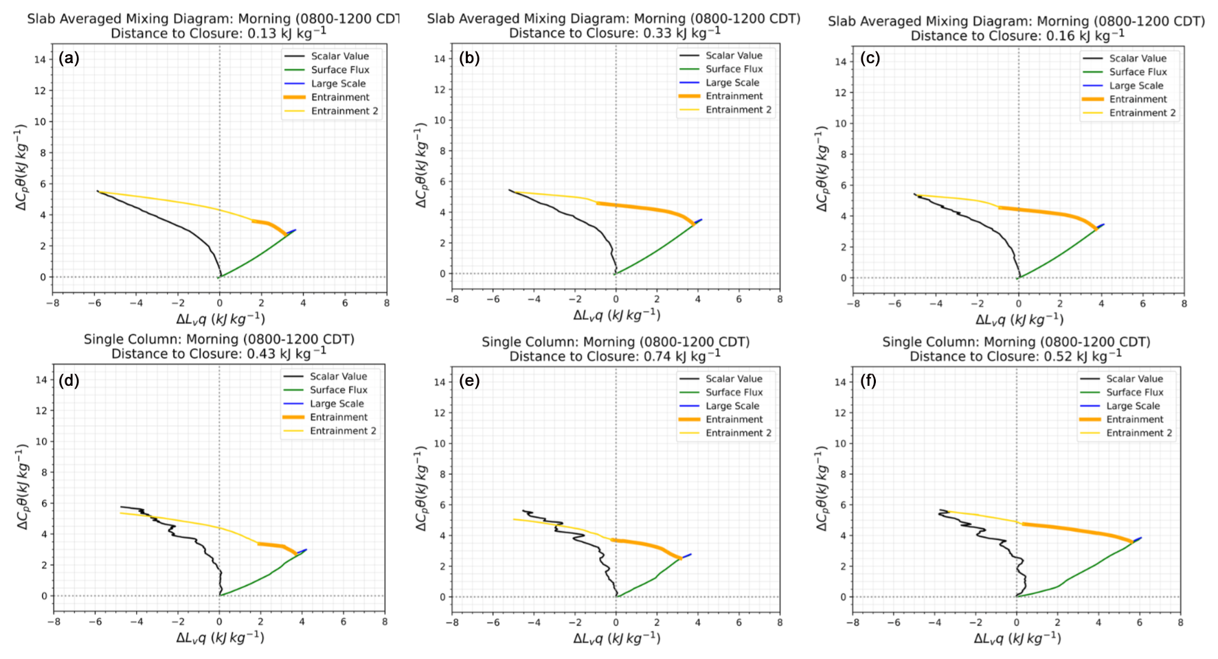
Figure 4 Mixing diagrams for the morning (08:00–12:00 CDT) of 8 August 2017 at SGP, comparing the impact of three different BL depth definitions: the level of neutral buoyancy of a surface-based parcel of air (a, d), the maximum humidity variance (b, e), and the minimum potential temperature flux (c, f), for the slab output (a, b, c) and the single-column output (d, e, f).

Figure 5 Same as Fig. 4 but for the afternoon time period (12:00–17:00 CDT).

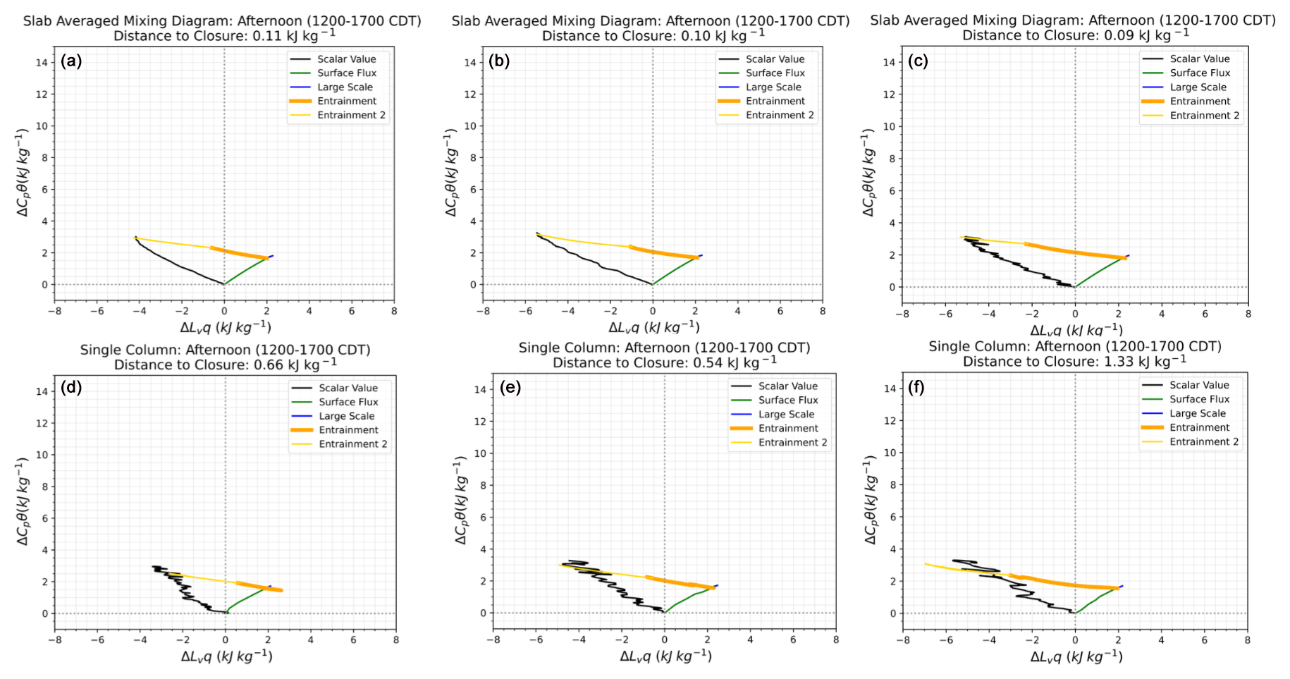
We see similar results during the afternoon time (12:00–17:00 CDT) (Fig. 5), where the overall magnitude of the total entrainment (ENT1 + ENT2) is the same regardless of boundary layer depth definition but the partitioning of the two terms changes with BL definition. During this time, the ENT2 term is largest using the maximum humidity variance definition. This is because, as we saw with the morning time, the ENT2 term is larger when z_i is located higher in the entrainment zone, and at 13:00 CDT the maximum humidity variance BL definition crosses the level of neutral buoyancy definition, making it higher in the atmosphere. The relative contribution of ENT1 to total entrainment remains the largest when the minimum potential temperature flux definition is used, and the ENT2 term is the smallest in that case. Interestingly, the ENT2 is never negligible during either analysis period for this day. This is because the BL depth is still growing the entire time, so the ENT2 term must be considered.

Figure 6 also shows differences in the morning and the afternoon. During the morning, there is not much of a pattern across the different dates of the different BL definitions, and the overall trend between the two ratios is mostly linear, but the ratios are not directly correlated. This is because the boundary layer is growing into the free troposphere. The evolution of the energy budget of θ and q_t is happening at different rates. In the afternoon, however, the trend across all of the dates and BL definitions is linear with very little deviation. This tells us that θ and q_t are evolving at the same rate in the afternoon.

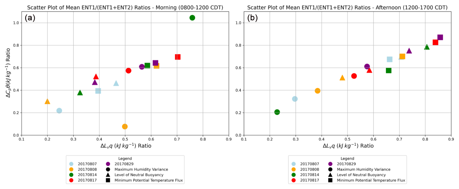
Figure 6 Ratio of ENT1 to (ENT1 + ENT2) for the morning (a) and afternoon (b) for Θ_t versus q_t. The different shapes are all five of the different dates considered, and the colors represent the three boundary layer depth definitions considered: the level of neutral buoyancy of a surface-based parcel of air (green), the maximum humidity variance (orange), and the minimum potential temperature flux (blue).

For both time periods, the single-column MDs are slightly different from the slab-averaged MD. It is difficult to capture the evolution of an entire horizontal domain from a single column, so differences between the two are to be expected. For both time periods, the partitioning between ENT1 and ENT2 is different for the maximum humidity flux and the minimum potential temperature flux cases in that the ENT1 term in the single-column MD is larger than the slab for both of those cases. This tells us that defining z_i as the level of neutral buoyancy, when calculated from that particular single column, is closer to the slab-derived level of neutral buoyancy BL definition than the respective maximum humidity variance and minimum potential temperature flux definitions. This could be due to the fact that the variance and fluxes are averaged from single-column output and then used to determine BL depth, while the level of neutral buoyancy definition uses direct single-column output. The following section dives deeper into the variability across different columns and dates, and the level of neutral buoyancy definition is used in the remainder of this study.

3.2 Mixed layer definition

ENT2 represents the change in BL properties due to the change in the BL depth over time. The value of a property at the top of the BL is not the same as that of the property within the mixed layer. This difference is more drastic the greater the change in the BL depth over time is. ENT2 is crucial for closure in the mixing diagram, as shown in the previous section, and is calculated by $\left(\frac{\partial z_i}{\partial t}-\stackrel{\mathrm{‾}}{w_i}\right)\frac{\left({\stackrel{\mathrm{‾}}{\mathit{\varphi }}}_{\mathrm{top}}-{\stackrel{\mathrm{‾}}{\mathit{\varphi }}}_{\mathrm{ml}}\right)}{z_i}$. The difficulty here is defining the “mixed layer”. The mixed layer could be considered to be the entire area below the top of the BL, or, as in W23, it could be defined as 0.1z_i−0.5z_i. These will be referred to as the full z_i and restricted definitions, respectively. Here we see which definition allows for a single column to better capture the slab ENT2. Figure 7 shows the second entrainment term for the morning (left) and afternoon (right) when the mixed layer is taken to mean the full z_i (gray) and when the mixed layer is restricted (0.1z_i−0.5z_i, orange +) for each column and compares them to the mean second entrainment term of the slab average (blue • and + for the full z_i and restricted cases, respectively). In the morning, both definitions of the mixed layer mean for individual columns cluster around the slab value in both sensible and latent heats, but the estimates of the ENT2 value is very different between the two methods. For the morning, the pairwise distance of the respective clusters is calculated – for the restricted method that distance is 1.28 (kJ kg⁻¹), and for the full method, that distance is 1.10 (kJ kg⁻¹). In the afternoon, there is much more overlap between the two different methods, though that overlap tends to underestimate both ENT2 contributions. The pairwise distance for the restricted method in the afternoon is 1.58 (kJ kg⁻¹), and for the full method, it is 1.45 (kJ kg⁻¹). It makes sense that the afternoon values would have more overlap between the two methods as the change in boundary layer depth over time is smaller in the afternoon, making the magnitude of ENT2 smaller at that time, so the restricted mixed layer would have similar values to the entire space below the BL during that time. In the remainder of this study, we use the full z_i method regardless of the time of day, as the cluster around the slab value in the morning is closer, according to the pairwise distance of farthest points in the cluster, for this method than for the restricted method, so single-column values do a slightly better job of capturing the slab ENT2 with that definition.

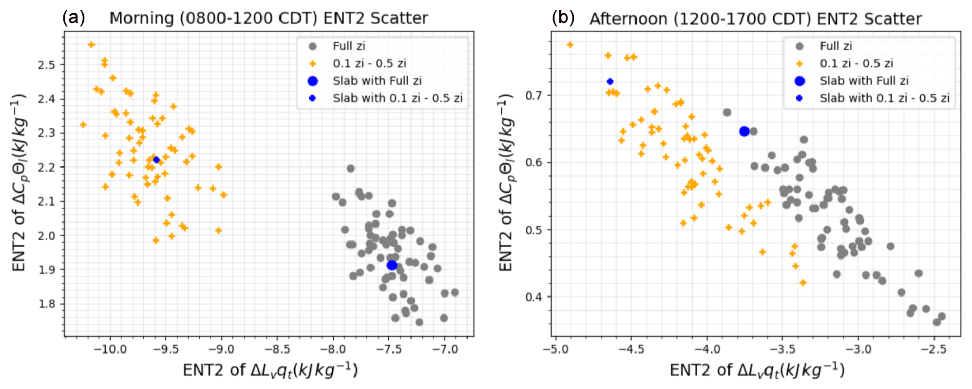
Figure 7 Comparison of the two different mixed layer definitions when calculating ENT2 for potential temperature and humidity for the (a) morning and (b) afternoon for 8 August 2017. The gray points are for when the mixed layer is taken as the entire area below z_i (full z_i), and the orange + symbol is from when the mixed layer is defined as 0.1z_i−0.5z_i (restricted) derived from each individual column in the domain. The respective slab ENT2 values are shown in blue.

3.3 Variability

No two columns will yield the exact same MD, due to sampling uncertainties. To get a sense of how well this MD framework behaves for many individual columns, we compare the closure of the sensible and latent heat terms for a set of columns and various cases. We look at the closure of the slab-averaged output, which is the LES slab-averaged statistical output and serves as the truth to which we compare all of the other closure values. Then, within the LES domain, we have 64 individual columns that serve as a proxy for observations. If we sum the data from those 64 columns and average over the horizontal domain, we get the closest to the slab data that we can get from the individual columns – we call this the average across single columns. Figure 8 shows the closure in the sensible and latent heats for the slab output (blue), from each individual column (gray), and the average across single columns (orange). The purple dot is the average of all of the closures of the individual columns (the average of all of the gray dots) and shows the general trend of all of the columns. The left plot is for the morning (08:00–12:00 CDT) and the right plot is for the afternoon (12:00–17:00 CDT) for 8 August. Ideally, our 64 individual columns would replicate the slab average (our “truth”) by temporally averaging single-column output. We see that during the morning (left), the average across the 64 columns and the average of all of the columns are very close. This means that the average single column will yield a similar closure value to the full array. In the afternoon, the average of all of the columns (purple) is closer to the slab value (blue) than the average across all 64 columns (orange), so for this case, the average single column replicates the slab values better than the result from averaging across the full array. A positive closure value means the residual underestimates the entrainment (i.e., the sum of the entrained heat and moisture is too small), while a negative closure value means the residual overestimates the entrainment (i.e., the sum of the entrained heat and moisture is too large). We see that in both the morning and the afternoon time periods, we have more variability (i.e., that the spread of the individual columns relative to the slab-averaged values is greater) in the latent heat than the sensible heat and that the average single column tends to underestimate the latent heat in relation to the slab-averaged value of the latent heat. These figures give us a sense of the sampling error. The spread of the individual columns serves as an indicator of maximum uncertainty in the sensible and latent heats. Figure 9 shows the mean closure value versus the number of columns used in calculating that closure across all five dates considered, over the entire day (08:00–17:00 CDT). For the most part, the more columns used, the smaller the closure value. This shows us that using multiple columns reduces the sampling error or that using multiple profilers, rather than one, would significantly reduce the sampling error.

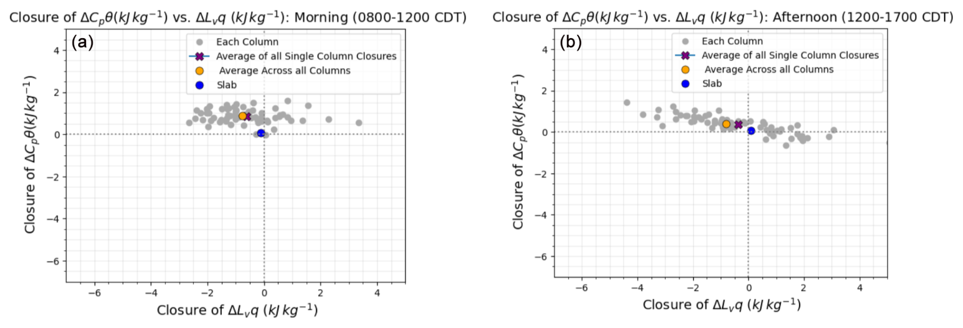
Figure 8 Scatter plots showing the closure in the sensible and latent heats for each single column (gray), the average of the closure values for all of the columns (purple), the average across all 64 columns (orange), and the slab average (blue) for 8 August during the (a) morning (08:00–12:00 CDT) and (b) afternoon (12:00–17:00 CDT). In the morning, the average of all of the columns (purple) and the average across all 64 columns (orange) points are on top of one another.

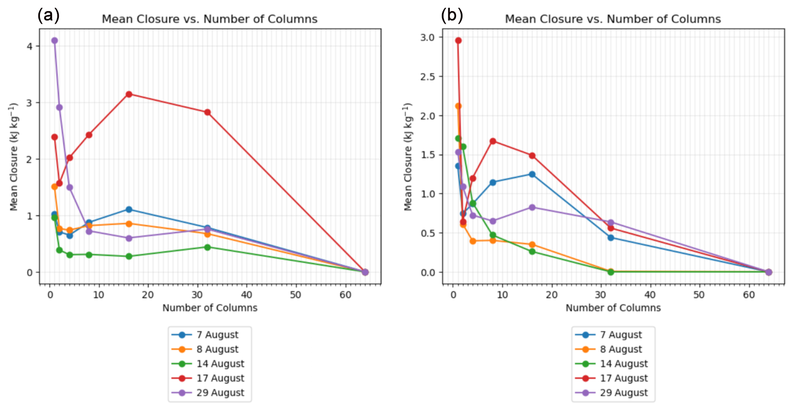
Figure 9 The mean closure value for a mixing diagram versus the number of columns used in calculating that closure for each of the five dates considered for (a) the morning and (b) the afternoon.

To see the closure trends and compare them across different dates, Fig. 10 compares the closure values for all five dates considered (7, 8, 14, 17, and 29 August 2017) for the morning (left) and the afternoon (right). The larger lines show the 1σ error bars on the single columns to better visualize the spread of the errors on each date. In the morning, the average across all of the columns is closer to the slab values with respect to the latent heat but underestimates the sensible heat. In the afternoon, we see that the average across all of the columns underestimates the sensible heat and tends to overestimate the latent heat across all of the dates. This is consistent with what we saw in Fig. 8, which confirms that our results are consistent across multiple dates.

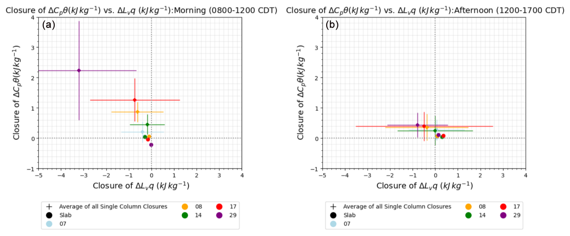
Figure 10 Comparison of the closure values averaged across all of the columns of each of the five dates considered (7, 8, 14, 17, and 29 August 2017) (purple +) with a 1σ uncertainty range and the slab-averaged closure values (blue •) for the (a) morning and (b) afternoon.

Some reasons for the discrepancies between the slab value and the column values could be that there is a bias imposed by temporally averaging the single-column data, the method for extrapolating single-column values to the surface varies, or the distance between the individual columns is large enough to not fully represent the domain.

4 Discussion

Deriving entrainment using the MD framework as a residual assumption is valid during time periods where the BL depth is changing; however, that residual term does not represent only the entrainment fluxes (ENT1) but the total entrainment (ENT1 + ENT2). ENT2 is crucial for closing a mixing diagram when the BL depth is changing. The magnitude of the total entrainment vector remains the same regardless of the BL depth definition being used, but the magnitudes of the individual terms change since different BL depth definitions sit in different positions within the entrainment zone. The magnitude of ENT2 is larger the higher in the entrainment zone the BL depth definition is. This means that the contribution to the total entrainment from ENT2 increases the closer to the free troposphere the BL depth definition is. Calculating ENT2 requires defining a mixed layer, and we found that using the full BL depth as the mixed layer definition yields results from a single column that are closer to that from the slab values than a previously identified range of 0.1z_i−0.5z_i, assuming there are no systematic errors in the mean profiles of θ and q over the depth of the convective boundary layer (which is why W23 used the restricted height definition for that analysis).

MDs can be used to describe the evolution of the heat and moisture budgets of the BL where the BL depth is quasi-stationary or changing with time, and this method can be applied to single-column output. The MDs derived from LES single-column output tend to underestimate the amount of sensible heat and overestimate the amount of latent heat when compared to the slab-averaged LES output. The disagreement is important because the slab output is the truth, and the difference from that truth serves as a method for determining sampling error. Ultimately, we see that there is less sampling error for sensible heat than latent heat and that there is more error in the latent heat in the afternoon than in the morning. The greater amount of sampling error in latent heat is expected because it is more sensitive to mixing with the free atmosphere at z_i than sensible heat. These results are consistent across multiple columns and multiple dates.

5 Conclusions

This work uses LES output as a test bed for determining entrainment from ground-based remote-sensing observations using a MD framework. By comparing results from proxy observations derived from LES single-column output to the LES slab-averaged output, we develop a method for applying a MD framework to morning hours and deriving total entrainment. We find that the residual from a MD framework represents the total entrainment and compares well with the actual sum of the entrainment terms ENT1 and ENT2. In the future, it is crucial to interpret the residual of a MD as the sum of both entrainment terms rather than the entrainment fluxes alone.

The magnitudes of the ENT1 and ENT2 terms are sensitive to BL depth definition, but the magnitude of total entrainment stays the same regardless of definition. Using a mixed layer definition of the entire BL allowed for better agreement in calculating ENT2 from the single-column and slab output. Finally, sampling error was estimated by determining the average closure value across multiple columns and across five individual dates, and we showed that the sampling error was larger for latent heat than for sensible heat.

Sampling error was reduced dramatically from a single column to multiple columns. This shows us that being able to average over more than one single column would be more representative of a selected region. The implications of this result for observations are that adding even a few more vertical profilers to a region could drastically reduce sampling error. This would lead to more accurate and representative observations in the future. Future modeling work should be done to determine an optimum number and spacing for profilers to best reduce sampling error.

These findings were all based on spatially homogeneous surface fluxes. Spatial heterogeneity would likely exacerbate our results of sampling error reduction with additional columns, as one column may be even less representative of an area in that case. Further work should be done in the future to determine the ways in which a heterogeneous surface would impact the overall evolution of sensible and latent heats throughout the day within the boundary layer.