Calibration of weather radars with a target simulator

We present findings from radar calibration experiments involving three radars operated by the Colorado State University (CSU) in the US and by the École Polytechnique Fédérale de Lausanne (EPFL) in Switzerland. The experiments were based on the comparison between measured radar variables and the known properties of artificial point targets electronically generated with a polarimetric radar target simulator (RTS) from Palindrome Remote Sensing. Radars under test included the two magnetron-based radars CHILL and SPLASH (its mobile version) from CSU and EPFL's new solid-state radar StXPol.

For the CHILL and SPLASH calibration measurements in Colorado, a mobile lifting platform was employed that elevated the target simulator instrument to approximately 15 m above ground. The creation of virtual targets with polarimetric signatures allowed for a direct calibration of polarimetric variables. While the SPLASH radar exhibited good Z_dr and sufficient Z_h accuracy, remarkable precision and stability were found in CHILL's reflectivity data time series, where the reflectivity bias compared to the virtual target was less than 0.2 dB over a 1 h time series.

Calibration issues that arise with solid-state radar systems were investigated with experiments conducted with the EPFL StXPol radar. This pulse compression system transmits a linear frequency-modulated long pulse as well as a non-modulated short pulse for observations at close ranges. The two pulses are separated in frequency by 50 MHz, and consequently calibration targets were generated independently for the two channels. Excellent stability and accuracy were found for Z_dr in both channels. While Z_h stability was also very high, a large reflectivity bias in both the long and the short pulse channel was detected.

For the first time, the article introduces and analyzes a weather radar calibration procedure that is based on electronically generated radar targets. Experimental data suggest that precise absolute and differential calibrations can be achieved if data are obtained in an environment free from multipaths and if the generated targets are precisely located in the center of the radar's range gate. Experimental shortcomings associated with limited sampling resolution of the radar scan over the targets are also investigated.

1 Introduction

Advancements in meteorological radar technology have broadened the applicability of weather radar data to a wealth of complex applications such as high-resolution nowcasting of precipitation, lightning or hazardous winds, combined rain gauge/weather radar quantitative precipitation estimation, hydrological runoff forecasts, radar data assimilation in numerical weather prediction models, and radar climatology. Therefore, the quality of weather radar data is critically important for weather services that provide advanced radar-derived meteorological and hydrological products to users. Not only advanced weather radar applications require highly accurate radar data: tasks like radar data exchange among national networks and the subsequent generation of radar mosaic products rely on radar data that are calibrated to the highest standards.

Focusing on the radar reflectivity, weather radar calibration involves all aspects of relating the received power that is backscattered by hydrometeors to the physical properties and the location of the hydrometeors. To be able to completely interpret the captured radar data, the full path must be characterized: from pulse generation to transmission, propagation, backscattering, reception, and digitalization (end-to-end calibration). In particular, the basis for the correct interpretation of the received radar signal is its amplitude relative to the transmitted signal. The ratio between the transmitted and received power can be determined by explicitly measuring powers, gains, and losses along the transmit and receive path. However, this is insufficient for advanced weather radar products that are based on dual-polarization measurements (Chandrasekar et al., 2015).

In this article, we present a dual-polarization radar target simulator (RTS) which is capable of generating electronic point targets with well-defined radar cross-section (RCS) and Doppler properties. These known artificial targets serve as a reference for the complete end-to-end calibration of a polarimetric weather radar.

Up to now, standard techniques for radar reflectivity calibration with point targets have employed external targets with known scattering properties, such as metal spheres and corner reflectors (Scarchilli et al., 1995; Joe and Smith Jr., 2001; Atlas, 2002). These metal spheres can be attached to balloons or drones (Bechini et al., 2010; Williams, 2013; van den Heuvel et al., 2018), facilitating this calibration technique. In Yin et al. (2019), Joshil and Chandrasekar (2022), and Ye et al. (2024) drone-based calibration processes are described in detail. The position of the sphere can be determined with a GPS sensor that is attached to the sphere. If a lifting platform is used, the rope lifting the calibration target must be sufficiently long so that the lifting platform does not contribute to the RCS.

Thanks to the relatively large beam width in the azimuth and elevation directions, trihedral corner reflectors have also been widely used for radar calibration purposes, mostly in synthetic aperture radar (SAR) and other space-based radar applications (Gray et al., 1990). A major source of error in ground-based configurations is the scattering contribution from the ground itself. For weather radar calibration, previous studies have attempted to limit ground reflections using corner reflectors mounted on high wooden poles (Martner et al., 2003) or on a tripod installed on a mountain ridge (Schneebeli et al., 2013).

The expected accuracy of these standard methodologies is of the order of 1 dB, mostly accounting for the uncertainties in the antenna pointing and the target location within the radar's pulse volume. In fact, the radar's matched filter transforms the incoming rectangular pulse shape that is reflected from the point target into a triangular power distribution that is spread over several range gates. If the point target is not exactly located in the center of the range gate, the theoretical radar reflectivity that is calculated from the target's RCS is higher than what is measured. The error caused by this uncertainty can be up to 6 dB in cases where the target has been placed exactly at the edge of a range gate.

End-to-end differential reflectivity (Z_dr) calibration can be obtained through different means, such as obtaining the differential antenna pattern with a box scan in the direction of the sun (Holleman et al., 2010; Frech and Hubbert, 2020) or the observation of light rain at vertical incidence, known as the bird-bath technique (Gorgucci et al., 1999). These techniques and their variants are implemented as regular scans in many operational weather radar networks (e.g., Louf and Protat, 2023). Although these techniques provide stable results, they do not allow investigating effects like Z_dr dependence on the differential phase or receiver nonlinearities that may cause Z_dr biases when the calibration target exhibits nonzero Z_dr properties.

The use of electronically generated targets offers several advantages, including greater control over target properties, improved precision, and the ability to eliminate positioning uncertainties. Their main advantage over static targets like metal spheres or corner reflectors is given by the fact that target properties can be changed such that calibrations can be made at different ranges, velocities, and radar cross-sections, which enables calibration measurements over the whole dynamic range of the radar receiver, as shown in Schneebeli et al. (2023a). Target simulators were employed for weather radar calibration purposes during site acceptance tests of the third-generation Swiss radar network (Gabella et al., 2013) (Germann et al., 2022) as well as during field campaigns (see, e.g., Gehring et al., 2021).

This study explores the advantages of using an RTS for the calibration of weather radars, ensuring accurate measurements of reflectivity, differential reflectivity, and Doppler velocity. Although differential phase measurements can also be performed with the instrument, as described in Schvartzman et al. (2024), this feature is not part of the current study. This article is organized to provide a systematic approach to radar calibration with RTS. Section 2 introduces the fundamental principles of weather radar calibration, discussing the importance of accurately interpreting backscattered signals from hydrometeors. Section 3 describes the operational aspects of the RTS, detailing how electronically generated targets provide a controlled and repeatable reference for calibration. The different radars under test are briefly presented in Sect. 4. The methodology employed in the calibration experiments is outlined in Sect. 5, highlighting the procedures for evaluating absolute reflectivity, differential reflectivity, and Doppler velocity accuracy. Finally, results from three distinct experiments, conducted on three different X-band weather radars, are presented in Sect. 6. As discussed in Sect. 7, the findings demonstrate the effectiveness of the RTS in identifying and correcting biases inherent to each radar system while also confirming the high temporal stability of measurements.

2 Electronically generated targets

An RTS is a system designed to create a simulated radar target at a specified range, incorporating a pre-defined Doppler shift and radar cross-section (RCS). In the case of a monostatic radar, the RTS captures the transmitted radar pulses, modifies them, and retransmits them with a time delay corresponding to the intended target distance on the radar display. This time delay Δt (s) is given by

$$\begin{array}{}\text{(1)}& {\displaystyle }{\displaystyle }\mathrm{\Delta }t={\displaystyle \frac{\mathrm{2}(r_t-r_s)}{c}},\end{array}$$

where r_t (m) represents the distance from the radar to the virtual target, and r_s (m) denotes the distance between the radar and the RTS.

To simulate a Doppler shift, the frequency shift f_D (Hz) applied to the reflected pulse is determined by

$$\begin{array}{}\text{(2)}& {\displaystyle }{\displaystyle }{f}_{\mathrm{D}}={\displaystyle \frac{\mathrm{2}v}{\mathit{\lambda }}},\end{array}$$

where v (m s⁻¹) represents the intended radial velocity of the simulated target, and λ (m) denotes the wavelength of the radar's carrier frequency.

Regarding the RCS, let $p_{\mathrm{r}}^{\text{RTS}}$ (W) denote the power of the radar pulse that is intercepted by the RTS. The power that is re-emitted by the RTS, $p_{\mathrm{t}}^{\text{RTS}}$ (W), is determined by the desired RCS, σ_b (m²). In particular, following Schneebeli et al. (2023a), the fraction

$$\begin{array}{}\text{(3)}& {\displaystyle }{\displaystyle }K={\displaystyle \frac{p_{\mathrm{t}}^{\text{RTS}}}{p_{\mathrm{r}}^{\text{RTS}}}}\end{array}$$

between the power transmitted and that received by the RTS is related to σ_b as

$$\begin{array}{}\text{(4)}& {\displaystyle }{\displaystyle }K={\displaystyle \frac{\mathrm{4}\mathit{\pi }{r_s}^{\mathrm{4}}{\mathit{\sigma }}_b}{{G_{\text{RTS}}}^{\mathrm{2}}{\mathit{\lambda }}^{\mathrm{2}}{r_t}^{\mathrm{4}}}},\end{array}$$

where G_RTS (–) represents the RTS antenna gain under the assumption that the gains of the RTS transmit and receive antenna are equal. The RTS setup that is used for the experiments presented in this article uses the same antenna for reception and transmission, and hence this assumption is valid. Inside the RTS, the incoming digital samples are scaled by an amplitude multiplication factor k at the voltage level, i.e., k²=K, and thus

$$\begin{array}{}\text{(5)}& {\displaystyle }{\displaystyle }k={\displaystyle \frac{\mathrm{2}\sqrt{\mathit{\pi }{\mathit{\sigma }}_b}{r_s}^{\mathrm{2}}}{G_{\text{RTS}}\mathit{\lambda }{r_t}^{\mathrm{2}}}}.\end{array}$$

If the power fraction K is accurately controlled, a target with an RCS σ_b can be generated, making it suitable as a calibration reference. However, in weather radar applications, the priority is to provide a reference target with a specific radar reflectivity. This requires generating a target with a defined RCS per unit volume, which in turn depends on the radar's pulse volume ΔV_p (m³). Assuming a Gaussian-shaped radar beam, ΔV_p can be expressed as (Probert-Jones, 1962)

$$\begin{array}{}\text{(6)}& {\displaystyle }{\displaystyle }\mathrm{\Delta }{V}_{\mathrm{p}}={\displaystyle \frac{\mathit{\pi }{\mathrm{\Theta }}^{\mathrm{2}}\mathrm{\Delta }r{r}_t^{\mathrm{2}}}{\mathrm{8}\ln \left(\mathrm{2}\right)}},\end{array}$$

with the half-power beam width of the radar antenna, Θ (rad), and the range extension of the pulse volume, Δr (m). Instead of applying the approximation for the pulse volume given in Eq. (6), which may lead to errors as high as 0.5 dB, it is more accurate to calculate the pulse volume from the normalized antenna pattern f(θ,ϕ) using

$$\begin{array}{}\text{(7)}& {\displaystyle }{\displaystyle }\mathrm{\Delta }{V}_{\mathrm{p}}=\int f^{\mathrm{2}}\left(\mathit{\theta },\mathit{\varphi }\right)\mathrm{d}\mathrm{\Omega }\mathrm{\Delta }r{r}^{\mathrm{2}},\end{array}$$

with elevation angle θ (rad), azimuth angle ϕ (rad), and solid angle differential dΩ≡sin θ dθ dϕ (sr).

Following standard weather radar textbooks (e.g., Rinehart, 1997), the relation between the effective radar reflectivity Z (mm⁶ m⁻³) and σ_b is written as

$$\begin{array}{}\text{(8)}& {\displaystyle }{\displaystyle }{\mathit{\sigma }}_b={\displaystyle \frac{Z{\mathit{\pi }}^{\mathrm{5}}{\left|\mathcal{K}\right|}^{\mathrm{2}}\mathrm{\Delta }{V}_{\mathrm{p}}}{{\mathit{\lambda }}^{\mathrm{4}}}},\end{array}$$

where |K|²=0.93 is a parameter associated with the complex refractive index of liquid water. Combining Eqs. (4), (6), and (8), the RTS power fraction K can be expressed as a function of the radar pulse width τ_pw (s), namely

$$\begin{array}{}\text{(9)}& {\displaystyle }{\displaystyle }{\mathit{\tau }}_{\text{pw}}=\mathrm{2}\mathrm{\Delta }r/c,\end{array}$$

along with the range variables r_s and r_t, the RTS antenna gain G_RTS, the beam width Θ, and wavelength λ of the radar under test.

3 Radar target simulator

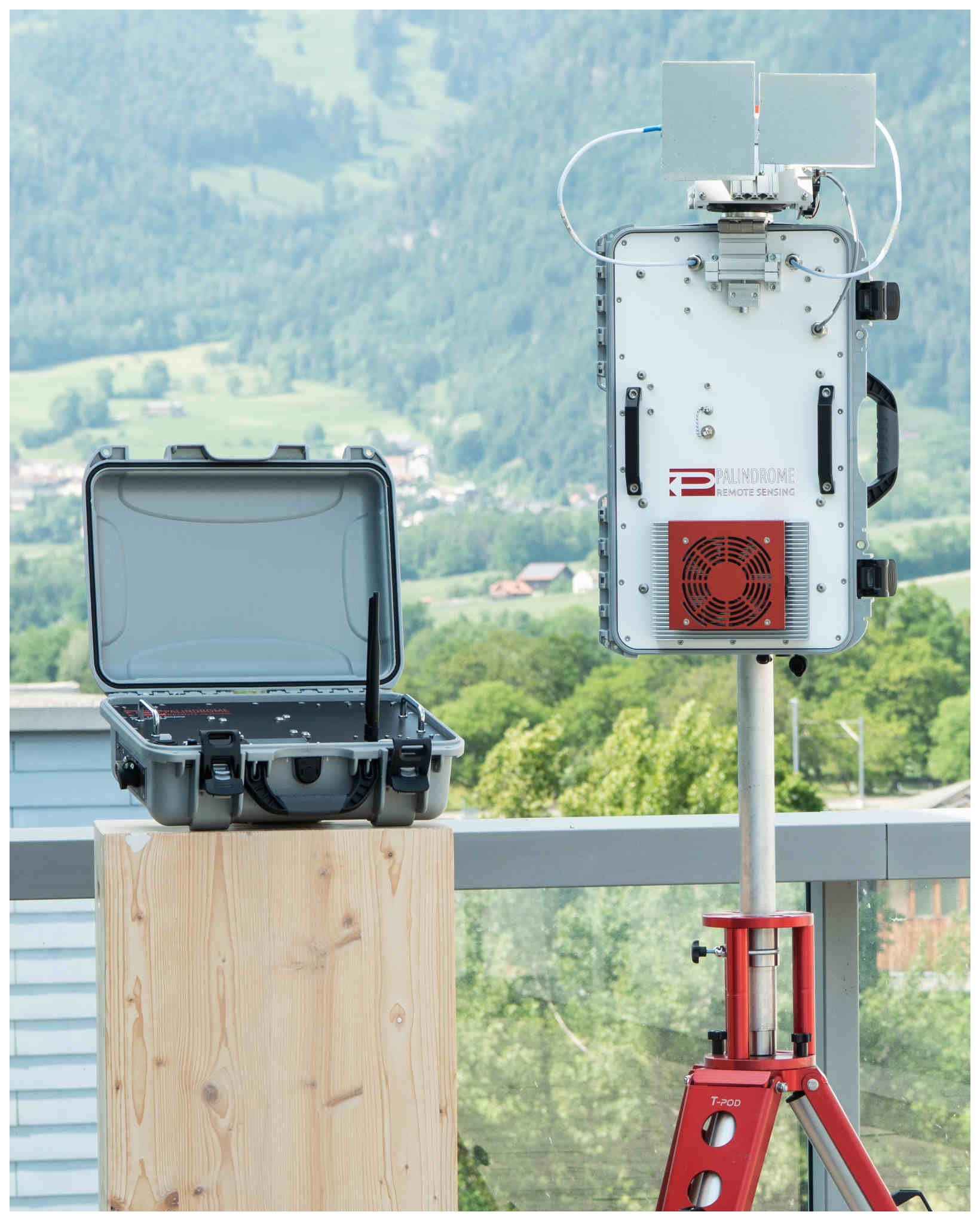
Palindrome p2q is a dual-polarization RTS developed for weather radar calibration. Its capabilities for calibrating and monitoring weather radars are described in Schneebeli et al. (2023a) and a photo of the instrument is provided in Fig. 1. The main purpose of the RTS is to retransmit the received signal in such a way that the power of the transmitted signal maintains a well-defined ratio to the power of the received signal. This ratio is referred to as the RTS factor K, as defined in Eq. (3). The RTS software automatically calculates K based on the pre-defined radar reflectivity (i.e., the desired cross-section of the simulated target) and the desired distance of the calibration target, the distance between the radar and the RTS, the radar's pulse width and its half-power beam width.

Figure 1 Close-up view of the RTS.

A basic description of the instrument together with an insight into its capability for measuring polarimetric phase differences is given in Schvartzman et al. (2024). The RTS receives radar pulses by either a polarimetric quad-ridged horn antenna with a gain of 13.8 dB (employed for the experiments in Colorado) or by two orthogonally aligned standard gain horns with a gain of 19.5 dB (employed for the experiments in Lausanne) and performs analog down-conversion over two frequency stages before IQ signal components are digitized and sampled at a rate of up to 100 MHz per channel. For the experiments described in this article, samples were acquired at a rate of 25 MHz. The digital radar pulses can be stored, modulated, and retransmitted with a given time delay while maintaining a pre-defined ratio between incoming and outgoing amplitudes. This enables polarimetric calibration targets with arbitrary reflectivity and Doppler characteristics to be generated.

In addition to weather radar calibration applications, the instrument has been employed for various radar testing tasks such as the calibration and commissioning of a multistatic C-band drone detection radar (Schneebeli et al., 2020, 2021, 2023b) as well as for the generation of radar signatures of wind turbines (Schneebeli and Leuenberger, 2021).

Figure 2 gives a schematic overview of the signal paths in the RTS. The labels and symbols used in this figure are described in Table 1. The RTS antenna is connected to the calibration units with RF cables. Since the signal path between the two is not calibrated during the operation of the RTS, it is important that high-performance cables are used, which maintain their pre-determined loss when the antenna is moved during the alignment procedure. The cable quality is even more important when the focus of the measurements is put on phase measurements, such as the experiment described in Schvartzman et al. (2024). To ensure phase and amplitude stability inside the RTS, all the critical analog parts like local oscillators, amplifiers, and the whole calibration unit are thermally stabilized at a temperature of 38 °C with an accuracy of 0.2 °C.

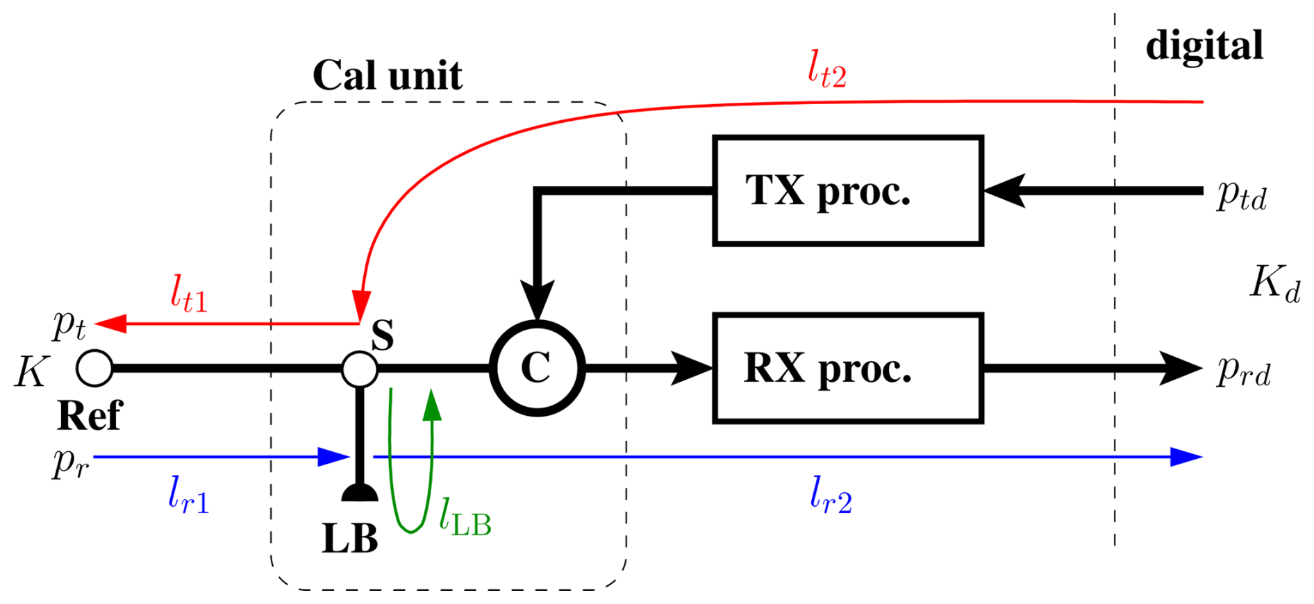
Figure 2 Schematic overview of the RTS signal paths. The description of the symbols is given in Table 1.

Table 1 Description and definition of the symbols shown in Fig. 2.

Precise alignment of the RTS antenna towards the radar under test is crucial for accurate calibration measurements since the gain of the RTS antenna is known only in the boresight direction. Correct pointing of the RTS antenna is ensured with an automated alignment algorithm: once the RTS is set up at its location, the radar under test points toward the RTS and starts to transmit in staring mode. The RTS antenna is mounted on a precision tracker which is capable of performing high-resolution box scans around the direction of the radar. Radar pulse power measurements that are acquired during the scanning procedure of the RTS antenna together with azimuth and elevation data of the RTS tracker lead to a Gaussian power distribution as a function of the tracker coordinates. With a 2D Gaussian fitting procedure the direction of the power maximum is determined in a straightforward manner. This direction then serves as the correct pointing direction from the RTS towards the radar.

The calibration of the RTS is divided into two processes: static and dynamic calibration. The static calibration, which is done once (or every few months) in the laboratory before the RTS is used in operation, compensates for the frequency-dependent losses between the calibration unit and the antenna, as well as the losses of the calibration loop-back. The dynamic calibration, on the other hand, is performed periodically during operation, usually every minute, and compensates for mainly temperature-induced variations of the gains and losses in the receive and transmit paths.

3.1 Operational mode

The digital loop-back factor K_d is the ratio of the digital transmit p_td to the digital receive power p_rd, namely

$$\begin{array}{}\text{(10)}& {\displaystyle }{\displaystyle }{K}_{\mathrm{d}}\equiv {\displaystyle \frac{p_{\text{td}}}{p_{\text{rd}}}}.\end{array}$$

This factor is controlled by the RTS software and adjusted after the calibration loop. In the receive path, the digital receive power p_rd is calculated as

$$\begin{array}{}\text{(11)}& {\displaystyle }{\displaystyle }{p}_{\text{rd}}=p_{\mathrm{r}}{G}_{\mathrm{r}\mathrm{1}}{G}_{\mathrm{r}\mathrm{2}},\end{array}$$

where G_r1 is the gain of the receive path between the reference point (Ref) and the switch (S), and G_r2 is the gain of the receive path between the switch (S) and the received digital signal. The transmit power p_t is computed as

$$\begin{array}{}\text{(12)}& {\displaystyle }{\displaystyle }{p}_{\mathrm{t}}=p_{\text{td}}{G}_{\mathrm{t}\mathrm{2}}{G}_{\mathrm{t}\mathrm{1}},\end{array}$$

where G_t1 and G_t2 are the gains of the transmit path between the switch (S) and the reference point (Ref) and between the transmitted digital signal and the switch (S), respectively. Combining Eqs. (3), (11), (10), and (12), the digital loop-back factor can be written as

$$\begin{array}{}\text{(13)}& {\displaystyle }{\displaystyle }{K}_{\mathrm{d}}={\displaystyle \frac{K}{G_{\mathrm{r}\mathrm{1}}{G}_{\mathrm{r}\mathrm{2}}{G}_{\mathrm{t}\mathrm{2}}{G}_{\mathrm{t}\mathrm{1}}}}.\end{array}$$

3.2 Dynamic calibration

During the calibration loop, a digital signal with power p_td,cal is generated in the field-programmable gate array (FPGA). It is reflected as an analog signal within the calibration unit, guided back into the receive path, and received again as a digital signal in the FPGA, denoted as p_rd,cal. The received power is calculated as

$$\begin{array}{}\text{(14)}& {\displaystyle }{\displaystyle }{p}_{\text{rd,cal}}=p_{\text{td,cal}}{G}_{\mathrm{t}\mathrm{2}}{G}_{\text{LB}}{G}_{\mathrm{r}\mathrm{2}},\end{array}$$

where G_LB is the gain of the loop-back path from the switch (S) to the loop-back (LB) and back to the switch (S). The ratio between the transmitted calibration power p_td,cal and the received calibration power p_rd,cal is the calibration constant K_cal.

$$\begin{array}{}\text{(15)}& {\displaystyle }{\displaystyle }{K}_{\text{cal}}\equiv {\displaystyle \frac{p_{\text{td,cal}}}{p_{\text{rd,cal}}}}={\displaystyle \frac{\mathrm{1}}{G_{\mathrm{t}\mathrm{2}}{G}_{\text{LB}}{G}_{\mathrm{r}\mathrm{2}}}}\end{array}$$

By using Eq. (13) to replace the term G_r2 G_t2, the digital RTS factor K_d becomes

$$\begin{array}{}\text{(16)}& {\displaystyle }{\displaystyle }{K}_{\mathrm{d}}=K{K}_{\text{cal}}{\displaystyle \frac{G_{\text{LB}}}{G_{\mathrm{r}\mathrm{1}}{G}_{\mathrm{t}\mathrm{1}}}}.\end{array}$$

3.3 Static calibration

The last term in Eq. (16) is assumed to be constant and must be measured before the instrument is used operationally:

$$\begin{array}{}\text{(17)}& {\displaystyle }{\displaystyle }{K}_{\text{static}}\equiv {\displaystyle \frac{G_{\text{LB}}}{G_{\mathrm{r}\mathrm{1}}{G}_{\mathrm{t}\mathrm{1}}}}.\end{array}$$

Considering both the static and dynamic configurations, the digital RTS factor is calculated as

$$\begin{array}{}\text{(18)}& {\displaystyle }{\displaystyle }{K}_{\mathrm{d}}=K{K}_{\text{cal}}{K}_{\text{static}}.\end{array}$$

3.4 Determination of the static calibration constant

The static calibration factor K_static can be determined by performing three measurements directly at the calibration unit. The first measurement is the gain of the receive path,

$$\begin{array}{}\text{(19)}& {\displaystyle }{\displaystyle }{A}_{\mathrm{r}}\equiv {\displaystyle \frac{p_{\text{rd}}}{p_{\mathrm{r}}}}=G_{\mathrm{r}\mathrm{1}}{G}_{\mathrm{r}\mathrm{2}},\end{array}$$

where the second equality follows from Eq. (11). The second measurement is the gain of the transmit path,

$$\begin{array}{}\text{(20)}& {\displaystyle }{\displaystyle }{A}_{\mathrm{t}}\equiv {\displaystyle \frac{p_{\mathrm{t}}}{p_{\text{td}}}}=G_{\mathrm{t}\mathrm{2}}{G}_{\mathrm{t}\mathrm{1}},\end{array}$$

where we used Eq. (12). The third measurement is the gain of the loop-back path,

$$\begin{array}{}\text{(21)}& {\displaystyle }{\displaystyle }{A}_{\text{LB}}\equiv {\displaystyle \frac{p_{\text{rd,cal}}}{p_{\text{td,cal}}}}=G_{\mathrm{t}\mathrm{2}}{G}_{\text{LB}}{G}_{\mathrm{r}\mathrm{2}}.\end{array}$$

See Eq. (14). The static calibration factor K_static can then be calculated as

$$\begin{array}{}\text{(22)}& {\displaystyle }{\displaystyle }{K}_{\text{static}}={\displaystyle \frac{G_{\text{LB}}}{G_{\mathrm{r}\mathrm{1}}{G}_{\mathrm{t}\mathrm{1}}}}={\displaystyle \frac{A_{\text{LB}}}{A_{\mathrm{r}}{A}_{\mathrm{t}}}}.\end{array}$$

The precise determination of K_static in the laboratory requires conducting the three distinct measurements outlined earlier, which necessitate the use of accurate RF measurement equipment. In our case, measurements were carried out using a signal generator capable of producing pulses with a wide range of amplitudes, along with a low-noise signal analyzer to detect weak pulses. If either the signal generator or the signal analyzer has calibration offsets, it is essential to compensate for these offsets dynamically throughout the measurement process. Furthermore, the measurement equipment must be synchronized to a common frequency reference. Cable losses and reflection coefficients (S₁₁ parameters) at the connection interfaces must also be considered to achieve measurement accuracies within 0.5 dB. As an alternative to using a signal generator and signal analyzer, K_static could also be determined with a vector network analyzer (VNA) capable of operating with pulsed signals.

3.5 Generating targets with a specific radar reflectivity

Inserting Eqs. (6), (8), and (9) into Eq. (4), the RTS power fraction K can be expressed written as

$$\begin{array}{}\text{(23)}& {\displaystyle }{\displaystyle }K={\displaystyle \frac{{\mathit{\pi }}^{\mathrm{7}}{\left|\mathcal{K}\right|}^{\mathrm{2}}{\mathrm{\Theta }}^{\mathrm{2}}Z{r_s}^{\mathrm{4}}c{\mathit{\tau }}_{\text{pw}}}{\mathrm{4}\ln \left(\mathrm{2}\right){G_{\text{RTS}}}^{\mathrm{2}}{\mathit{\lambda }}^{\mathrm{6}}{r_t}^{\mathrm{2}}}}\end{array}$$

as a function of the radar reflectivity Z. Some of involved quantities can be precisely configured in the RTS, such as r_s and r_t, whereas others, like G_RTS, must be known beforehand. Additionally, the parameters Θ and λ can be determined using the RTS itself. The radar wavelength is normally well-known before any measurements and does not need to be measured separately using the RTS. On the other hand, τ_pw and Θ are important to verify for the amplitude calibration of radar reflectivity using a target simulator. If the Gaussian beam approximation is not used, then the entire antenna pattern must be considered to compute the pulse volume as given in Eq. (7).

While measuring τ_pw is generally straightforward, as discussed in Sect. 5.2, determining the radar's Θ presents more challenges. The easiest approach is to use manufacturer-provided data. However, if these data are unavailable or unreliable, Θ must be determined separately through dedicated box scans around the generated target. Since simulated radar targets are point targets, their shape directly reflects the main beam pattern of the radar, making it possible to derive Θ, as demonstrated in Schneebeli et al. (2023a). It was found that the standard deviation of σ_Θ=0.02° inherent in successive measurements of Θ results in a reflectivity error of approximately 0.14 dB.

With reference to the computation of K according to Eq. (23), note that it is common that the pre-defined reflectivity of the calibration target often needs to be slightly adjusted a posteriori in case the analysis of the obtained pulse and radar data shows that the radars' real pulse width differs from the nominal one or if other settings were not fully correct during the experiment. The relevant parameter that is controlled by the RTS is always K and the corresponding reflectivity can be corrected if necessary during the analysis of the data. For instance, such corrections need to be applied if the distance r_s or the pulse width τ_pw differs from the RTS settings during the calibration experiment.

For system calibration, the relevant polarimetric radar variables are found in the direction where reflectivity reaches its peak. This direction can be identified by directly locating the maximum reflectivity in the radar data or by applying a Gaussian fit to the data beforehand. A statistically robust calibration is then achieved through a series of repeated sector scans.

3.6 Target distance effects

To calibrate the radar reflectivity Z using a point target, it is crucial to ensure the target is accurately positioned at the center of the range gate. A point target, when detected using a perfectly rectangular pulse, produces a parabolic response curve after matched filtering, similar to a triangular response in the voltage domain with a base width twice the pulse width. Since the radar's range resolution corresponds to the pulse width, there is a high probability that a point target will be sampled away from its peak response. This issue is mitigated by adjusting the target's range while maintaining its radar reflectivity.

This matched filter effect is illustrated in Fig. 3 where data from the StXPol radar (see Sect. 4) have been used. A static target was generated at various distances from the radar while its reflectivity was kept constant at all positions. The target's normalized amplitude in the voltage domain as detected by the radar is plotted as a function of the target range. By applying a triangular least-square fitting procedure to the measured data and evaluating the width of the fitted triangle at half of its maximum, the width of the matched filter can be experimentally inferred. In the data depicted in Fig. 3, this width was determined to be 156.8 m, which is very close to the nominal range gate size of 150 m corresponding to the employed pulse width of τ_pw=1 µs.

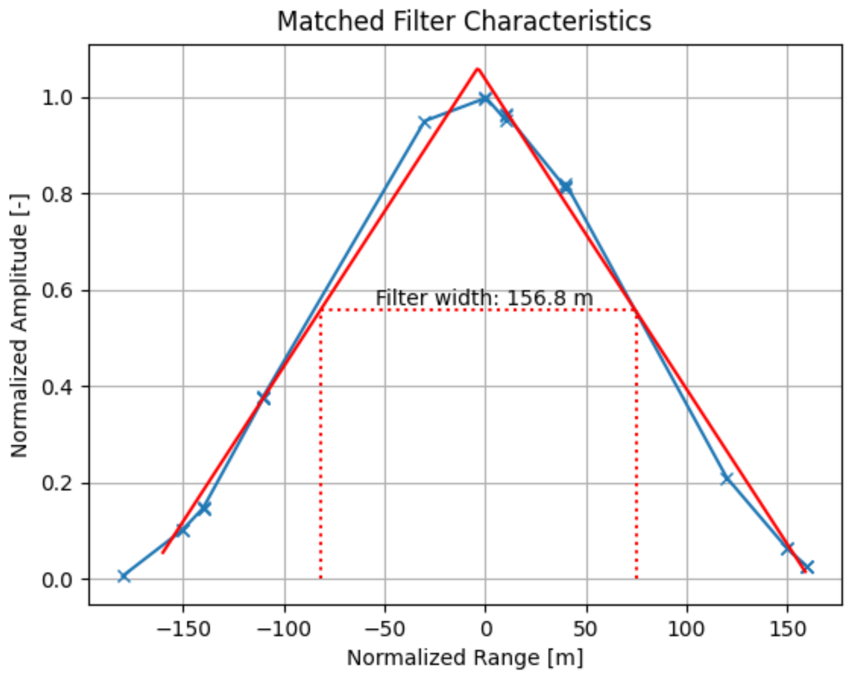
Figure 3 Matched filter characteristics inferred from a constant reflectivity target that was moved in range.

4 Radars

In this study, three X-band radar systems were employed together with the RTS: the CSU CHILL radar, the CSU SPLASH radar, and the StXPol system developed by ProSensing Inc. These radars represent a range of capabilities and configurations, each suited to specific observational needs and environmental conditions. The following sections provide an overview of each system's technical specifications, operating modes, and unique features relevant to the deployment and data collection efforts described in this work.

4.1 CHILL

The CSU CHILL radar is an S- and X-band system that has been thoroughly described in the literature (e.g., Bringi et al., 2011; Junyent et al., 2015). In the described experiment, only CHILL's X-band system has been used, which consists of a magnetron transmitter and a polarimetric receiver that are mounted on a Gregorian dual-offset antenna with gain of 53 dB. The radar's main characteristics are provided in Table 2.

Table 2 Specifications of the three radars used in the present study.

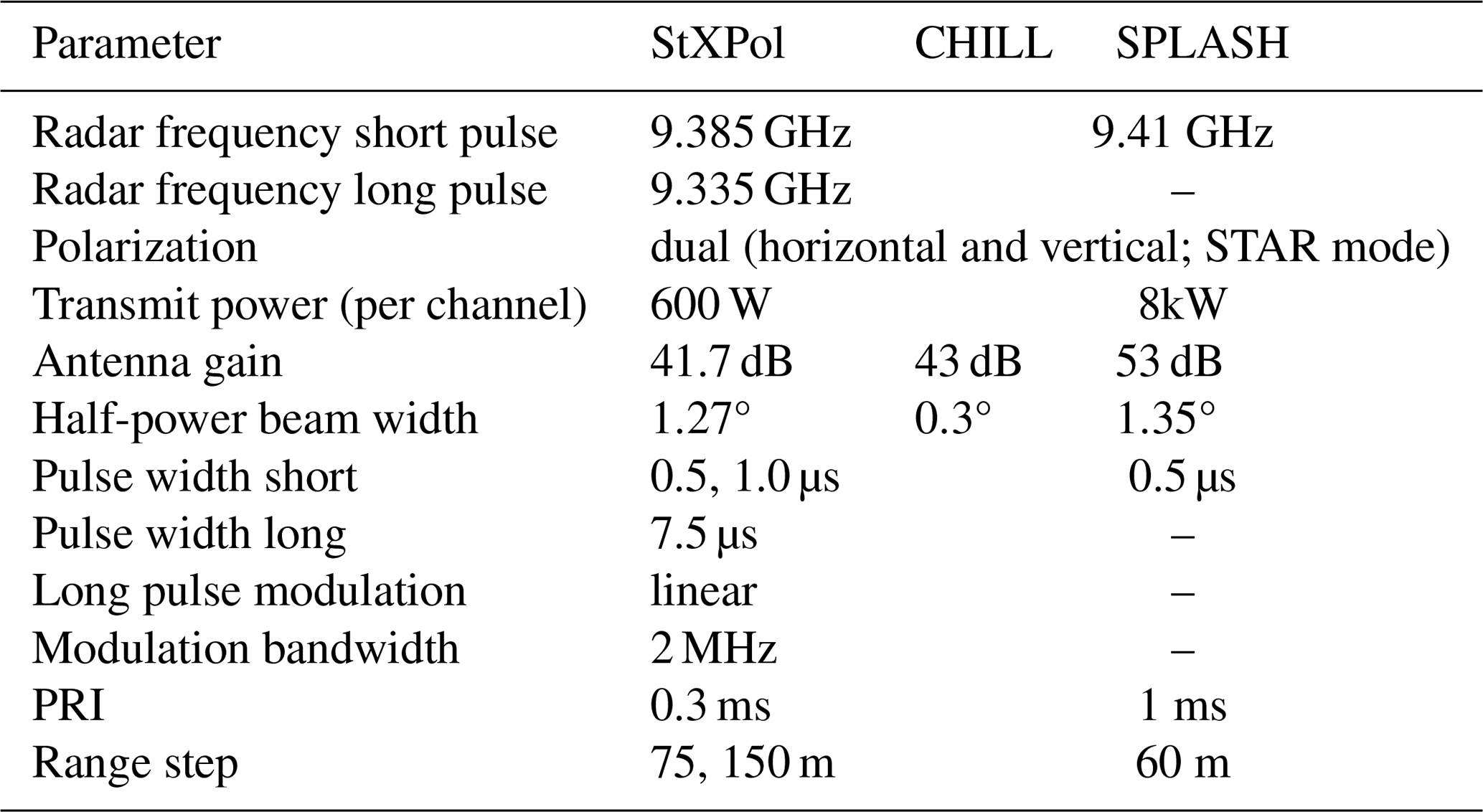
4.2 SPLASH

The CSU SPLASH radar is a dual-polarization Doppler weather radar designed for dense network deployments. It is similar to RXM-25, which is described in Galvez et al. (2013). Operating at X-band, it covers up to 50 km with range resolutions below 40 m and simultaneously transmits and receives horizontal and vertical polarizations.

The radar uses a low-cost magnetron transmitter delivering 12 W per polarization channel with a peak power output of 8 kW. A dedicated signal path and digital frequency tracking system adjust the receiver settings in real time. Its analog parallel receiver includes low-noise amplifiers, a GPS-disciplined reference oscillator, and a high excess noise ratio (ENR) noise source for internal calibration. The digital receiver provides digitized IQ signals and radar metadata over a 1 GB Ethernet link.

All signal processing and radar control run on a single server, handling real-time spectral processing, Doppler velocity unfolding, clutter filtering, and attenuation correction. The system supports both manual GUI-based and automated command-line operation, with automatic data transfer capabilities. All electronics are housed in enclosures that can be pressurized, allowing operation in harsh conditions without a radome. More detailed radar characteristics are given in Table 2.

4.3 StXPol

The Solid State X-band scanning Polarimetric radar (StXPol) built by ProSensing Inc. for EPFL is a radar system intended to provide measurements of clouds and precipitation and specifically designed to sustain high wind conditions and harsh cold environments in mountainous and polar regions. Able to operate in STAR (simultaneous transmission and receive) or alternate modes, it was employed in these tests in the former setting. It is equipped with a 1.82 m antenna (41.7 dB gain) and two 630 W solid-state amplifiers. The other radar main characteristics are provided in Table 2.

5 Experiments

Calibration experiments with the three radars were conducted at two locations. SPLASH and CHILL were tested at the CHILL radar facility in Greely, Colorado, whereas StXPol was tested at the EPFL campus in Lausanne, Switzerland. For the experiments in Colorado, Fig. 4 shows how the RTS was lifted to a height of approximately 15 m with an elevated platform. The distance of the RTS to the SPLASH and CHILL radar was 470 m. The experiments with the SPLASH and CHILL radar were conducted in September 2023. For the experiment on the EPFL campus, the RTS was deployed from the roof of a building that was located at a distance of 356.7 m from the radar. Experiments with StXPol were conducted during 1 d in November 2023 and repeated on a later day in April 2024. Repetition was necessary to prove that reflectivity discrepancies between the short and the long pulse channel can be associated with the non-centered placement of the calibration target within the range gate.

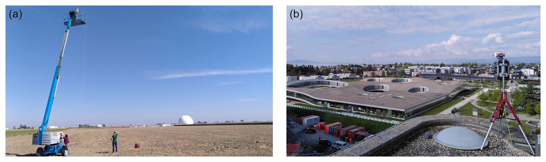
Figure 4 (a) Target simulator on the elevated platform with CHILL and SPLASH in the background. (b) Experimental setup in Lausanne.

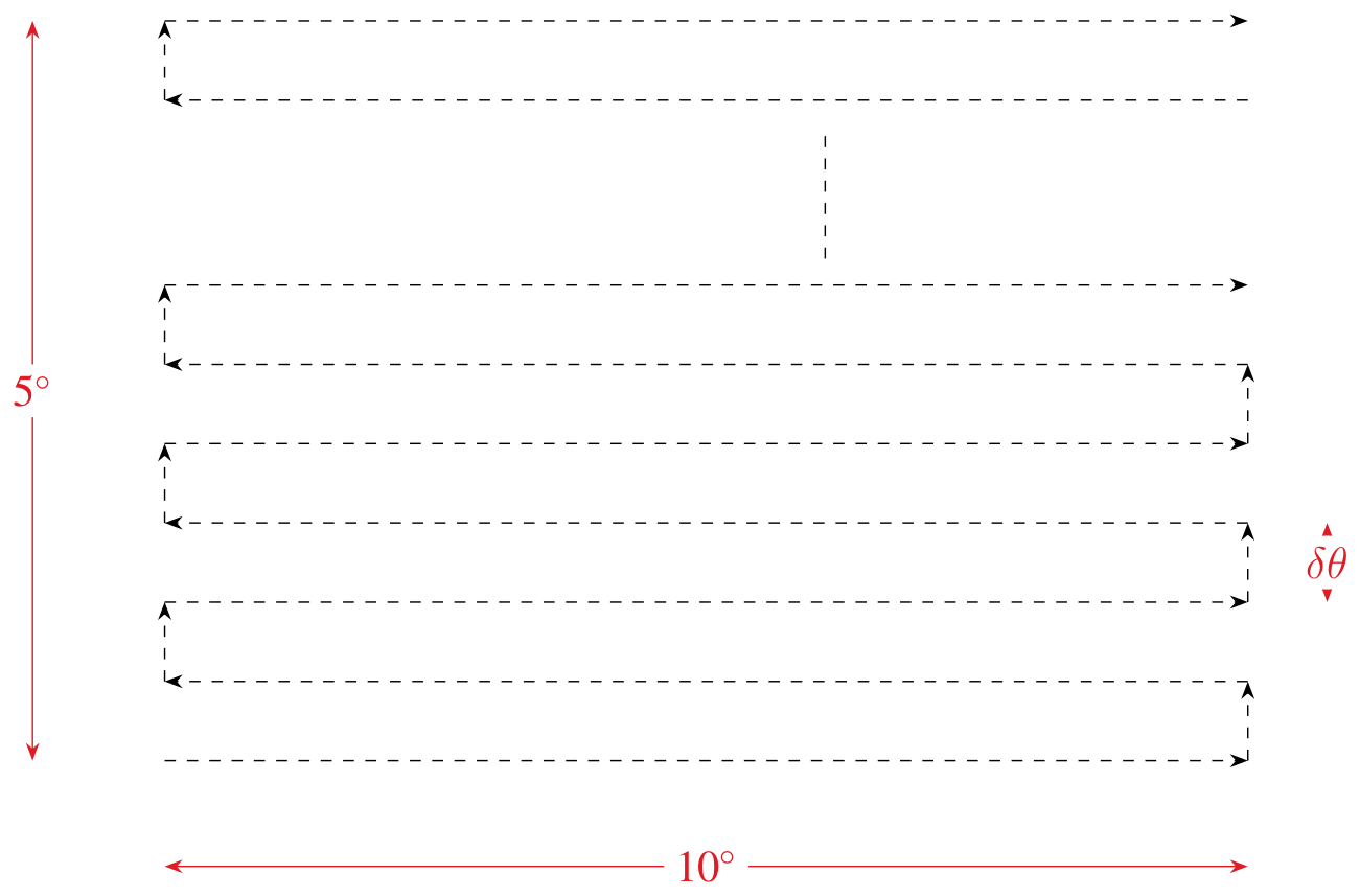
5.1 Scan strategy and data acquisition

The sketch of the radar scan strategy is shown in Fig. 5 for the StXPol and SPLASH radars. The scan consisted of 25 subsequent sector scans that were spaced in elevation by δθ=0.2° for SPLASH and StXPol and δθ=0.1° for CHILL. The antenna speed was set to approximately 1° s⁻¹ such that one full box scan was completed in slightly less than 5 min. The start elevation was 0°.

Figure 5 Illustration of the box scan that is performed around the virtual target.

Box scan data were extracted at the range gate that exhibited the highest reflectivity. A 2D Gaussian fitting procedure was applied to the linear (i.e., non-logarithmic) reflectivity values of the box scan. The maximum of the fitted reflectivity is considered to be the relevant measured reflectivity that needs to be compared to the pre-defined target reflectivity. For other polarimetric or Doppler properties that need to be compared to the RTS values, a 2D Gaussian averaging kernel is constructed from the previously fitted reflectivity. If $\widehat{Z}(\mathit{\theta },\mathit{\varphi })$ designates the fitted reflectivity value when the radar points in the direction (θ,ϕ), the averaging kernel is defined as

$$\begin{array}{}\text{(24)}& {\displaystyle }{\displaystyle }{L}_{\text{av}}(\mathit{\theta },\mathit{\varphi })={\displaystyle \frac{\widehat{Z}\left(\mathit{\theta },\mathit{\varphi }\right)}{{\sum }_{\mathit{\theta }}{\sum }_{\mathit{\varphi }}\widehat{Z}\left(\mathit{\theta },\mathit{\varphi }\right)}}.\end{array}$$

Calling B(θ,ϕ) the measured value of the polarimetric or Doppler observable of interest at the radar's pointing direction (θ,ϕ), we compute the following weighted estimate of the observable of interest:

$$\begin{array}{}\text{(25)}& {\displaystyle }{\displaystyle }{b}_{\text{av}}=\sum _{\mathit{\theta }}\sum _{\mathit{\varphi }}{L}_{\text{av}}(\mathit{\theta },\mathit{\varphi })B(\mathit{\theta },\mathit{\varphi }).\end{array}$$

With the CHILL radar, only six sector scans with a spacing of 0.1° in elevation were obtained for one repetition. Because of the size of the CHILL radar antenna, its far field is located at approximately 4.8 km, while the target simulator was set up at a distance to the radar of 470 m. In consequence, it is expected that the beam is not yet properly formed away from the center axis and therefore does not exhibit its final narrow shape yet. Nevertheless, it can be assumed that one sector scan hits the RTS with sufficient accuracy. The subsequent analysis of the CHILL data is therefore based on only one sector scan that was performed at an elevation of 0.68°.

5.2 StXPol pulse measurements

5.2.1 Pulse power

During the StXPol experiments, the power of the radar pulses that were sampled with the RTS was continuously and accurately determined in an absolute manner thanks to an update of the RTS firmware that allowed the comparison of incoming power with an internal reference pulse source. Although such absolute power measurements are unnecessary for reflectivity calibration tasks, where only the fraction between the incoming and outgoing RTS power is relevant, the additional quantitative data provide useful information on the radar performance as well as on potential multipath contamination. Some of the acquired StXPol pulse measurements are therefore detailed as follows.

Figure 6 shows the shape of the short pulse in the left panel and a series of maximum pulse power amplitudes over the suite of two sector scans in the right panel. An important and obvious feature of both figures is the fact that the data from the two RTS channels overlap very well. This not only indicates that the two radar channels transmit an equal amount of power, but it is also a first confirmation that measurements are not affected by multipath contamination because the two polarizations are unlikely to be equally affected by the multipath.

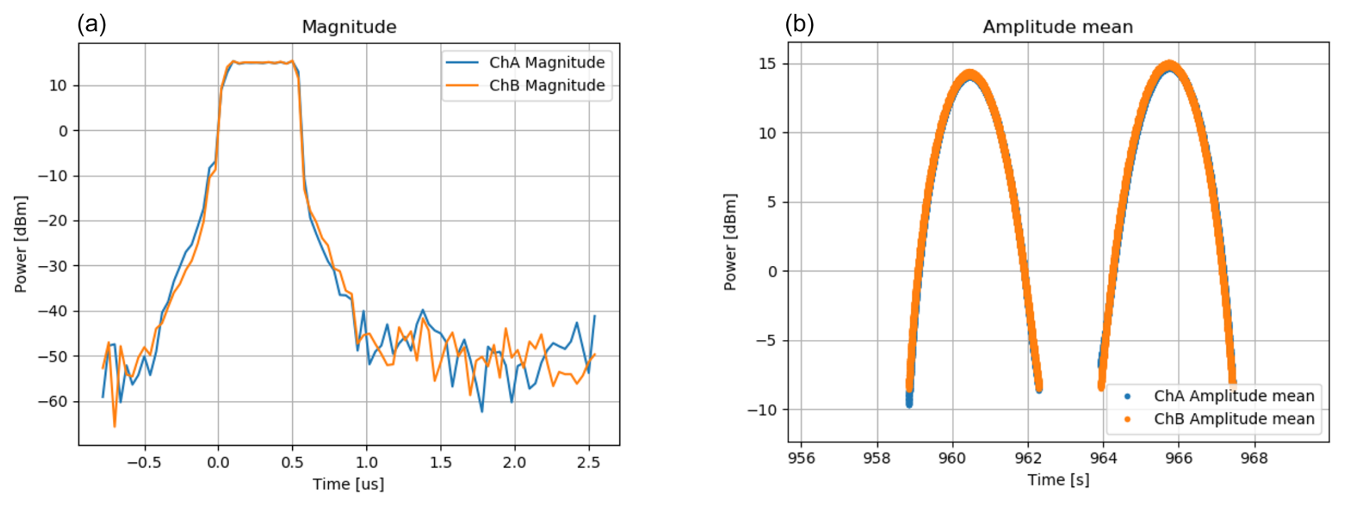
Figure 6 (a) Shape of the StXPol short pulse for both polarizations. (b) Pulse power maximum for both polarizations over two consecutive sector scans.

The two sector scans exhibit the RTS maximum receive power P_rts, and hence it can be used to estimate the radar transmit power P_rad according to the Friis transmission equation (e.g., Ulaby and Long, 2014):

$$\begin{array}{}\text{(26)}& {\displaystyle }{\displaystyle }{P}_{\text{rad}}={\displaystyle \frac{P_{\text{rts}}}{G_{\text{rad}}{G}_{\text{rts}}{\left(\frac{\mathit{\lambda }}{\mathrm{4}\mathit{\pi }{r}_s}\right)}^{\mathrm{2}}}},\end{array}$$

where G_rad=41.7 dB and G_rts=19.5 dB are the antenna gains of the radar and the RTS, respectively, and r_s=356.7 m is the distance between the radar and the RTS. With P_rts=14.9 dBm (determined from the maximum value of the right panel of Fig. 6) a value of P_rad=472.34 W is calculated, which corresponds to the transmit power of one polarization right behind the radar antenna. This value can be compared with the direct measurement made 1 d later with the spectrum analyzer at the waveguide that feeds the radar antenna. With the spectrum analyzer, a value of P_rad=501 W was obtained, which amounts to a difference of 0.25 dB between the two methods. Since this difference is small, it is concluded that multipath effects that might affect pulse amplitudes can be neglected.

5.2.2 Pulse modulation

The cumulative phase of a linear frequency-modulated (LFM) chirp is supposed to exhibit a parabolic shape. The image given in the right panel of Fig. 7 depicts the measured cumulative phase of the radar's modulated long pulse with a nominal bandwidth of 2 MHz. The shown parabolic phase behavior Φ(t) can be described as

$$\begin{array}{}\text{(27)}& {\displaystyle }{\displaystyle }\mathrm{\Phi }\left(t\right)={\left(t-{\displaystyle \frac{{\mathit{\tau }}_{\text{pw}}}{\mathrm{2}}}\right)}^{\mathrm{2}}{\displaystyle \frac{\mathrm{4}{\mathrm{\Phi }}_{\text{tot}}}{{\mathit{\tau }}_{\text{pw}}^{\mathrm{2}}}},\end{array}$$

with pulse width τ_pw and total cumulative phase Φ_tot. The frequency hub f_hub is calculated from Eq. (27) as

$$\begin{array}{}\text{(28)}& {\displaystyle }{\displaystyle \frac{\mathrm{1}}{\mathrm{2}\mathit{\pi }}}\left({\left.{\displaystyle \frac{\mathrm{d}\mathrm{\Phi }\left(t\right)}{\mathrm{d}t}}\right|}_{t={\mathit{\tau }}_{\text{pw}}}-{\left.{\displaystyle \frac{\mathrm{d}\mathrm{\Phi }\left(t\right)}{\mathrm{d}t}}\right|}_{t=\mathrm{0}}\right)={\displaystyle \frac{\mathrm{4}{\mathrm{\Phi }}_{\text{tot}}}{\mathit{\pi }{\mathit{\tau }}_{\text{pw}}}}=f_{\text{hub}}.\end{array}$$

This result together with the measurement of Φ_tot=652° (determined from the beginning and the minimum of the parabolic given in Fig. 7) leads to a modulation bandwidth of f_hub=1.937 MHz if a pulse width of τ_pw=7.4805 µs is assumed. The determined value of the modulation bandwidth is close to the nominal value of 2 MHz. It is therefore assumed that the correct pulse compression ratios were applied to the reflectivity data provided by the radar.

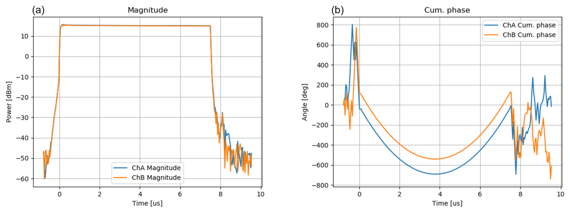
Figure 7 (a) Shape of the StXPol long pulse for both polarizations. (b) Cumulative phase over one long pulse duration for both polarizations.

6 Calibration results

6.1 StXPol

Since StXPol possesses two independent signal processing chains per polarization, i.e., one for the unmodulated short pulse (SP) and another for the frequency modulated long pulse (LP), calibration measurements were performed individually and sequentially for both channels with the different modulation schemes. A priori, it was not known that these two channels (SP and LP) exhibit a slight difference in range that might be induced by filtering effects. This range discrepancy requires that the placement of the generated target is individually adjusted for the two channels in order to locate the target exactly at the range gate center, as shown in Fig. 3. This matched filter effect deteriorates the accuracy of the absolute calibration but in principle does not effect the calibration of the differential reflectivity, Z_dr.

Regarding the first experiment in November 2023, the target range was set to 10.13 km, which is optimized for the LP channel. Due to an error in the target simulator software, the transmit path amplifier settings of the RTS were beyond optimal in the LP measurement setup, causing digital noise in the generated target and a reduced signal-to-noise ratio (SNR) in the corresponding radar data. This effect was manifested in the maximum values of the generated targets' co-polar correlation coefficients, ρ_hv: for SP a value of ${\mathit{\rho }}_{\text{hv}}^{\text{SP}}=\mathrm{0.996}$ was achieved, while for LP a value of ${\mathit{\rho }}_{\text{hv}}^{\text{LP}}=\mathrm{0.9984}$ was found. The reduced SNR negatively impacted Z_dr much more than the absolute reflectivity, and hence it was decided to only keep the LP measurements from November 2023 for absolute reflectivity calibration. The SP measurements from November 2023 exhibited a slight range offset, but SNR was excellent and therefore these measurements were only used for differential reflectivity calibrations.

As for the tests conducted in April 2024, SNR was excellent for both LP and SP, but this time the LP measurements exhibited the range offset. Therefore, Z_dr could be calibrated for both pulse lengths and only SP data were considered for absolute reflectivity calibration.

Relevant StXPol calibration results for absolute and differential reflectivity are provided in Table 3. The RTS power fraction, K, is provided for absolute reflectivity calibrations only and not for differential reflectivity, where the absolute value of K is irrelevant. In addition, the standard deviation of the time series of measurements is calculated only if more than three box scans per target were completed.

Table 3 StXPol reflectivity calibration results.

6.1.1 Reflectivity

An example of a box scan radar reflectivity acquisition performed around an electronic target that was generated for the short pulse channel is shown in Fig. 8. The target intensity was set to 60 dB. The maximum of the Gaussian fit (red contour lines in Fig. 8) assumed a value of 55.1 dB and hence a large reflectivity bias can be diagnosed.

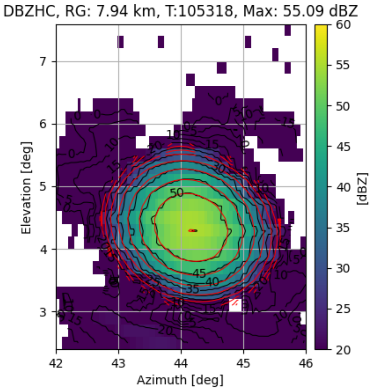
Figure 8 Reflectivity data obtained from a box scan around the virtual target that was generated at a distance of 7.86 km with a reflectivity of 60 dBZ.

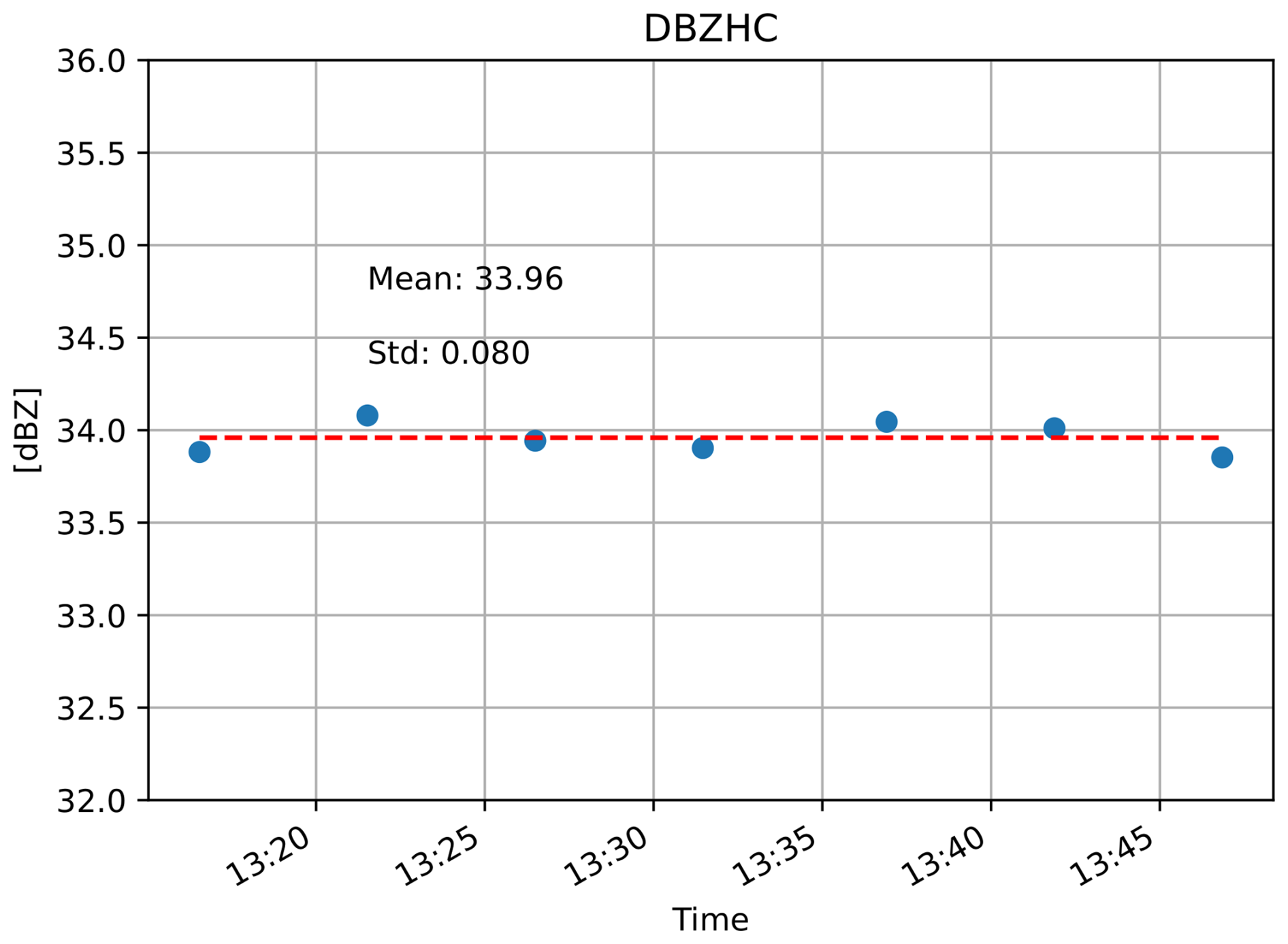
A similar reflectivity bias was found in the November 2023 experiment in the long pulse channel, as seen in Fig. 9. For the time series shown, seven box scan repetitions were performed around a target with a pre-defined reflectivity of 39.5 dBZ. The plotted data points correspond to the maximum of the Gaussian fit applied to the linear 2D reflectivity data. In this experiment, the target size was initially set to 40 dBZ but was corrected afterwards since the radar–RTS distance was not set correctly during the experiment.

Figure 9 Reflectivity time series of a target with a size of 39.5 dBZ.

Direct comparisons between the short and long pulse channel cannot be made, since it was found that a range offset of 40 m persists between the two channels. Since the target range was optimized for the long pulse channel in November 2023 and for the short pulse channel in April 2024, a calibration offset of approximately 2 dB between the two channels is found for each of the 2 d, which is explained with the plot shown in Fig. 3.

Despite these experimental shortcomings, the reflectivity bias remained consistent over the two experiments that were separated by 4 months. In addition and as seen in Fig. 9, the short-term stability was high. The reflectivity standard deviation of 0.08 dBZ, determined from time series data during the November 2023 experiment, was found to be similar for the SP and LP channel.

6.1.2 Differential reflectivity

A box scan acquisition of the differential reflectivity is given in the left panel of Fig. 10, while the right panel provides the corresponding time series. The data shown were acquired with the short pulse channel in November 2023, with the differential reflectivity of the target set to 0 dB.

Figure 10 (a) Differential reflectivity pattern of a box scan acquired with the short pulse. (b) Time series of the differential reflectivity where the target Z_dr was set to 0 dB.

The box scan plot exhibits a distinctive pattern that subdivides the Gaussian antenna pattern into four quarters. This pattern is assumed to be induced by the four struts of the antenna that hold the feed in place. Similar patterns were observed with solar box scans obtained with a C-band radar of the German weather service in Hohenpeissenberg (Frech and Hubbert, 2020), and additional directional biases can be caused by radomes with nonrandom geometric patterns (Figueras i Ventura et al., 2021). Since solar measurements are only passive, the magnitude of the antenna effect is smaller than for the active measurements used in our case. It is noteworthy that a value of Z_dr=0 dB is achieved only in the main beam direction of the antenna. With the averaging kernel method described in Eqs. (24) and (25), the box plot data are weighted in order to obtain the individual data point for the time series given in the right panel of Fig. 10.

The low bias and the high short-term temporal stability suggest that the radar is well-calibrated with respect to the differential reflectivity. For the LP data, a similar data acquisition procedure exhibited a Z_dr bias of 0.5 dB.

Up to this point, and also for the subsequent analysis of the differential reflectivity calibration for SPLASH and CHILL, the simplest case with a target exhibiting a differential reflectivity value of Z_dr=0 dB was used. In principle, there is no reason to believe that a dependence exists between the Z_dr value of the target and the respective calibration biases. However, given that the effects of polarization channel coupling on the Z_dr bias were investigated in many articles (e.g., Wang and Chandrasekar, 2006; Zrnić et al., 2010), it seems meaningful to perform calibration measurements with Z_dr targets that are different from 0 dB. To do so, three targets with Z_dr values of −4, 2, and 4 dB were generated, where the targets with the negative Z_dr exhibited a horizontal reflectivity of 60 dBZ, while the target with the negative Z_dr exhibited a horizontal reflectivity of 50 dBZ. The data stem from the short pulse channel and were collected in April 2024. The respective box scans can be seen in Fig. 11. The overall bias of these three acquisitions is −0.095 dB and hence a difference of 0.15 dB in the Z_dr bias between the 0 dB targets and the nonzero dB targets can be stated. From the authors' point of view, the number of scan repetitions is too low and the variance in the target properties too high to draw more detailed conclusions than the statement that no significant change in the Z_dr bias can be associated with a change of the target's Z_dr.

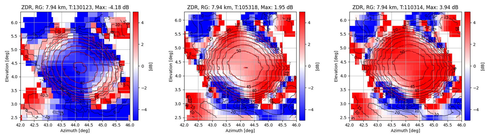
Figure 11 From left to right: box scans of Z_dr around targets that were generated with differential reflectivity values of −4, 2, and 4 dB.

6.1.3 Velocity

Doppler velocities can be attributed to electronically generated point targets in a very precise manner. Likewise, weather radars are capable of measuring Doppler velocities very precisely. For instance, StXPol's velocity bias was found to be lower than 0.01 m s⁻¹. Velocity calibration is therefore usually unnecessary. Many advantages are associated with generated targets that exhibit specific Doppler properties. Since the radar can be operated with a Doppler filter to further eliminate unwanted ground reflections, it is meaningful to test the behavior of this filter, as demonstrated in the left panel of Fig. 12. The radar pointed directly towards the RTS without moving its antenna (i.e., staring mode). While the generated target reflectivity remained constant, the target speed was reduced from 4 to 0.1 m s⁻¹. The radar's Doppler filter was set to a width of 0.83 m s⁻¹. It is observed that the suppression of targets with velocities that are within the filter width is not very sharp. In addition to theoretical verification of filter behavior at the signal processing level, this technique – based on generated targets that can be tuned to specific Doppler properties – provides the only means of thoroughly testing the implementation of the radar's Doppler filter.

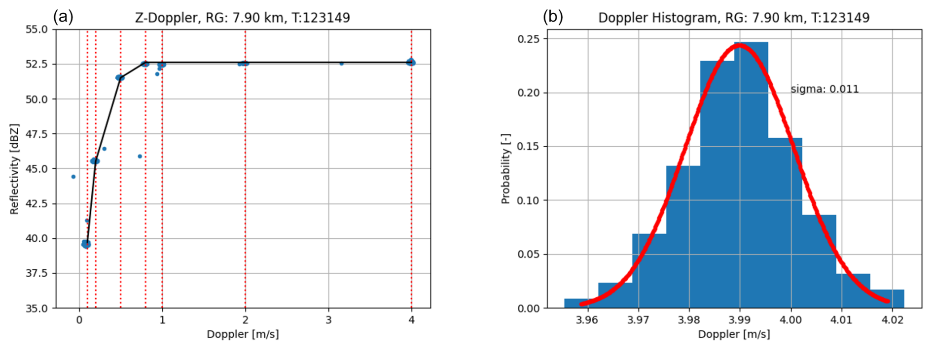
Figure 12 (a) Filter curve of a 0.83 m s⁻¹ wide clutter filter that was tested with a stable reflectivity target with changing Doppler properties. The red lines indicate the Doppler speeds that were given to the target. (b) Histogram of the same data as shown in the panel on the left-hand side, but extracted around a Doppler speed of 4 m s⁻¹. Data were acquired in FFT mode.

The Doppler time interval histogram can be determined from the same measurement by extracting data around a specific Doppler velocity. For the histogram that is plotted in the right panel of Fig. 12, reflectivity data that originate from a 4 m s⁻¹ Doppler target are used. We find a narrow Gaussian distribution with a width of 0.011 m s⁻¹. The nonzero spectrum width stems from phase noise contributions of the transmitter, the radar receiver, and the RTS phase noise. It is important to note that this histogram is not identical to the Doppler spectrum. The Doppler spectrum width was obtained with the radar during the scanning process and resulted in a value of 0.2 m s⁻¹ for an antenna speed of 1° s⁻¹. While the histogram shows how the mean of the Doppler spectra is distributed, one cannot infer one from the other. However, it shows that the spectral width that is inherent in the measurements is much wider than the fluctuations of the maxima and hence underlines that very precise Doppler measurements are obtained with the radar.

Figure 13 finally shows the box scan acquisition of the co-polar correlation coefficient, ρ_hv, which offers a practical way to assess imperfections in beam matching and low channel isolation. Virtually generated polarimetric radar targets and low-intensity stratiform rain are supposed to exhibit perfect correlation between the polarimetric channels. Values below 1 are caused by receiver noise and antenna performance, as stated in Mudukutore et al. (1995). Values as high as ρ_hv=0.9995 for the long pulse channel and ρ_hv=0.9996 for the short pulse channel were obtained, both with low standard deviations over time of the order of ${\mathit{\sigma }}_{{\mathit{\rho }}_{\text{hv}}}\sim {\mathrm{10}}^{-\mathrm{5}}$. The remarkably large and temporally stable nature of ρ_hv of a bright scatterer has been reported in Gabella (2018, 2021) where it was concluded that this quantity can be used for monitoring hardware deficits.

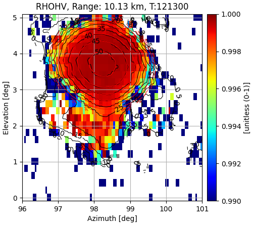
Figure 13 Radar measurements of the co-polar correlation of the virtual target. Measurements acquired with the short pulse are shown.

6.2 CHILL

The RTS was set up at a distance of 470 m to the radar at a height of approximately 15 m above ground. A photo of the experimental setup is shown in the left panel of Fig. 4. In contrast to the box scan data acquisition that was performed for SPLASH and StXPol, relevant data were extracted from one of six sector scans that were made in the direction of the RTS. A vertical cut through the sector scans at the location of the generated target is shown in Fig. 14. CHILL's large antenna and its narrow beam width of 0.3° facilitate the identification of slight pointing errors. As seen in the right panel of Fig. 14, the reflectivity is slightly shifted away from the direction of the antenna movement due to a gear backlash of 0.15°.

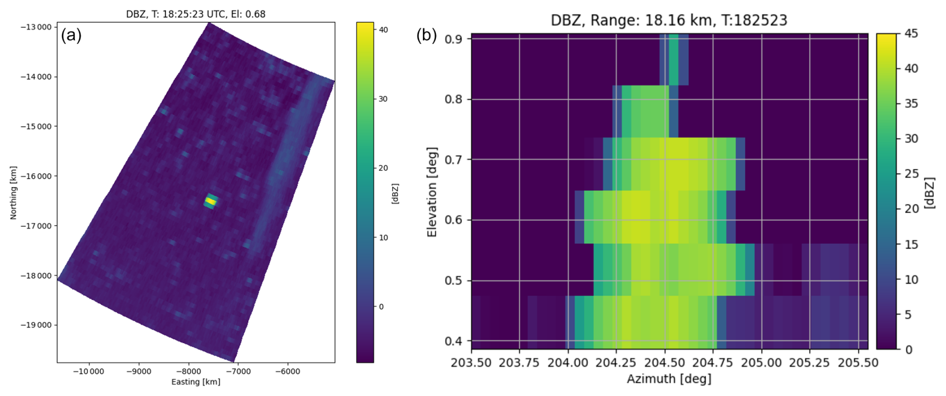
Figure 14 (a) CHILL radar reflectivity sector scan at the elevation of the RTS. (b) Vertical cut of CHILL reflectivity data through six sector scans extracted at the location of the generated target.

Similar to the procedure detailed for the StXPol radar, the target also had to be placed in the center of the range gate. As seen on the sector representation of the reflectivity data in the left panel of Fig. 14, the two range gates that are adjacent to the center range gate both exhibit similar reflectivity values, which indicates that the target was correctly placed in the range gate's center.

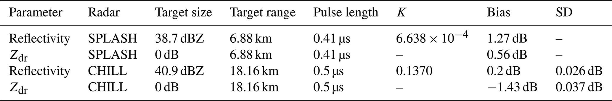
For reflectivity calibration purposes, a 40 dBZ target at a range of 18 km was generated. The initially chosen reflectivity value had to be corrected to 40.9 dBZ due to changes in the definition of the pulse volume. More specifically, the relevant RTS power fraction was set to a value of K=0.1370. This value, together with the RTS antenna gain $G^{\text{RTS}}=-\mathrm{6.36}\mathrm{dB}$, the distances r_s=470 m and r_t=18.01 km, and the pulse width τ_pw=0.5 µs, leads to the indicated reference reflectivity of the generated target. The reason that $G^{\text{RTS}}=-\mathrm{6.36}\mathrm{dB}$ is so low is due to the fact that an additional 20 dB attenuator was placed between the antenna and the reference point Ref (see Fig. 2). This was done to protect the RTS from the strong radar power from CHILL, owing to the high antenna gain of 53 dB and the short distance between the RTS and the radar antenna. The value of the attenuator was accounted for in the RTS antenna gain with $G^{\text{RTS}}=\mathrm{13.64}\mathrm{dB}-\mathrm{20}\mathrm{dB}=-\mathrm{6.36}\mathrm{dB}$, with 13.64 dB being the antenna gain of the quad-ridge horn antenna at a frequency of f=9.41 GHz, as determined in a calibration laboratory.

It is important to note that the RTS was set up in the radar's near field. The far field of the X-band CHILL radar starts at approximately 4.8 km, significantly beyond the radar–RTS distance of 470 m. However, it is not expected that this fact induces shortcomings for absolute reflectivity calibration measurements.

A 1 h reflectivity time series was collected from sector scans that were performed at an elevation of 0.68°. The radar's reflectivity data underwent a 1D Gaussian fitting procedure, after which the maxima of the fitted curves were used to produce the plot shown in Fig. 15. The extracted radar data (mean: 41.1 dBZ) exhibit good agreement with pre-defined target reflectivity and the temporal stability is very high over 1 h (standard deviation: 0.026 dB).

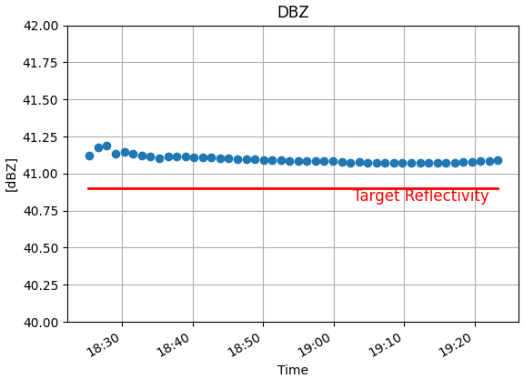
Figure 15 Time series of the maximum of a Gaussian-fitted sector scan over a generated point target.

An overview of the reflectivity calibration results can be found in Table 4. Slightly less convincing are the results for the differential reflectivity, Z_dr. Although the stability over 1 h was again very high, with a standard deviation in Z_dr as low as 0.037 dB, the bias of −1.43 dB in differential reflectivity is considerable. At the time of writing the origin of this bias has not been fully identified. An almost identical setup for the SPLASH calibration experiment, which was conducted just 1 d before the CHILL measurements, provided reasonable Z_dr calibration data. It is therefore assumed that the generated calibration target exhibited correct differential reflectivity properties. However, CHILL's extremely narrow antenna beam width of 0.3° makes the differential reflectivity calibration with a point target very demanding. The chosen scanning resolution in elevation of 0.1° is likely to be too low for accurate Z_dr calibration since the antenna beam center might have been missed by some hundredth of a degree. While the impact of this effect on the absolute reflectivity is low, it is considerable for Z_dr due to its high variation within the antenna beam. This can be illustrated by using the sector scan at an elevation of 0.78°, i.e., 0.1° above the scan that is used for the current analysis. By using this scan, the mean of the Z_dr time series is calculated to be 4.2 dB. It is speculative to calculate a mean from this value and the Z_dr value from the sector scan below, but the large difference between the two values serves as an indication that for future experiments, a higher scan resolution would be appropriate for such a narrow antenna beam width.

Table 4 CSU radar calibration results.

6.3 SPLASH

An experiment similar to the one with the CHILL radar was conducted on 13 September 2023 with the SPLASH radar. This mobile radar is very similar to the X-band CHILL radar, with the antenna being the main difference. SPLASH was set up close to CHILL such that the radar–RTS distance was r_s=431 m. The target's radar reflectivity at horizontal polarization was initially set to Z_h=40 dBZ but had to be corrected in the analysis to Z_h=38.5 dB. This was due to a correction of r_s and a difference between the measured and nominal values of the pulse width (0.41 µs and 0.5 µs, respectively). The relevant RTS power ratio was set to $K=\mathrm{6.638}{\mathrm{10}}^{-\mathrm{4}}$. The half-power beam width Θ of the radar antenna was obtained from the 2D Gaussian fit of the reflectivity (as shown in Fig. 16). By taking into account that Θ is inferred as the 6 dB beam width from the radar reflectivity, a value of Θ=1.35° was obtained in this manner. Box scans around the generated target were performed similarly to those for the StXPol experiment.

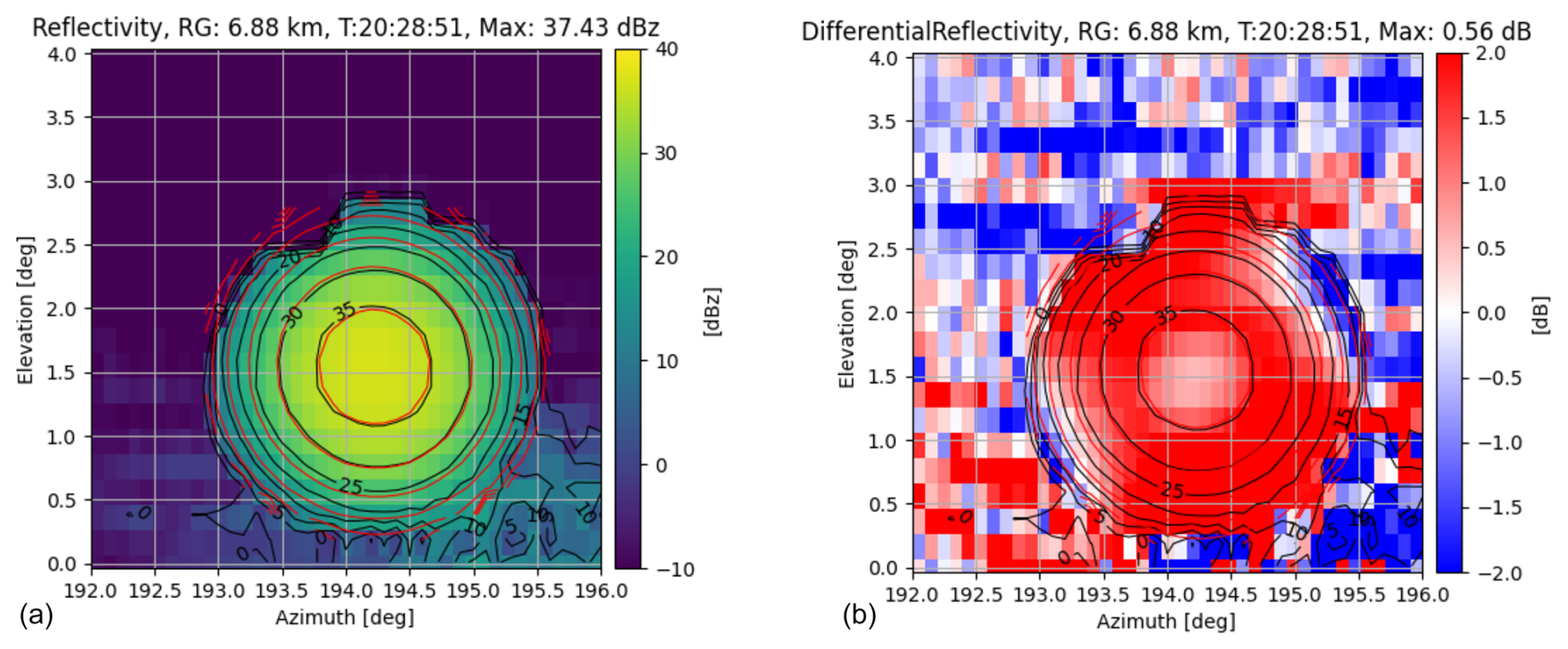
Figure 16 Reflectivity data obtained from a box scan around the virtual target that was generated at a distance of 6.88 km with a target reflectivity of 38.7 dBZ and a differential reflectivity of Z_dr=0 dB.

The box scan of the reflectivity data shown in Fig. 16 exhibits some missing data at the upper left corner of the target. The reason for this feature is the internal calibration procedure of the RTS that was executed when the radar was pointing in this direction. As seen from the contour lines of the measured reflectivity data (black) and the contour lines of the Gaussian fit (red), the fitting procedure is only marginally affected by this effect. In fact, the reflectivity representation of the generated target exhibits a distinctive regular Gaussian behavior, which justifies the usage of these data for the determination of the half-power beam width of the radar antenna. The maximum of the reflectivity fit was found at $Z_{\mathrm{h}}^{\text{max}}=\mathrm{37.43}\mathrm{dBZ}$ such that the reflectivity bias was calculated to be 1.27 dB. A standard deviation of this value is not given in Table 4, since only two box scan repetitions with the same target properties were conducted.

The value that is relevant for the calibration of the radar differential reflectivity, Z_dr, is extracted from the data shown in right panel of Fig. 16 with the abovementioned averaging kernel method (see Sect. 5.1). For a target with a nominal differential reflectivity of Z_dr=0 dB, a differential reflectivity offset of 0.56 dB is found from the depicted box scan. An apparent difference in the differential reflectivity patterns between SPLASH and StXPol can be noted. In order to fully explain the two patterns, a detailed investigation requiring measurements of co- and cross-polar antenna patterns would be necessary. With the data at hand, it is speculated that the two antennas exhibit different co- and cross-polar radiation patterns, with the cross-polar maximum located on the co-polar main lobe for the SPLASH antenna and four equal cross-polar maximum lobes arranged around the co-polar main lobe for the StXPol antenna, as depicted in Zrnić et al. (2010). The four cross-polar maxima with alternating phases can explain the four distinct Z_dr features located at elevations of 3.75 and 5.75° and azimuth angles of 42.5, 45.5, and 5.75° in Fig. 11. These features are absent in the right panel of Fig. 16, where a circular Z_dr minimum in the center of the radiation pattern is found instead.

Obtaining differential power measurements from box scans of the sun could potentially help to further analyze the differences found in Figs. 10 and 16. Differential power measurements of the sun have previously been made and are well-documented in the literature (Holleman et al., 2010; Moisseev et al., 2010; Reimann and Hagen, 2016; Frech and Hubbert, 2020). The study of Reimann and Hagen (2016) proposes the measurement of the magnitude and phase of the polarimetric correlation coefficient from the box scan of the sun, which yields information on the cross-polar isolation and therefore the cross-polar antenna pattern. These additional measurements could provide a valuable source of information for the interpretation of the different Z_dr patterns. It is proposed that such cross-polar measurements, obtained either with the sun or the target simulator itself, should be performed in upcoming experiments. For the presented experiments these data were not available.

6.3.1 Phase-based measurements

Apart from the clutter filter testing in Sect. 6.1.3, the main focus of the measurements presented up to now has been on power-based radar observables. To present a complete view of the measurement capabilities of an RTS, Fig. 17 depicts box scans of the radar's differential phase Ψ_dp, the Doppler spectrum width σ(v_D), and the Doppler velocity v_D.

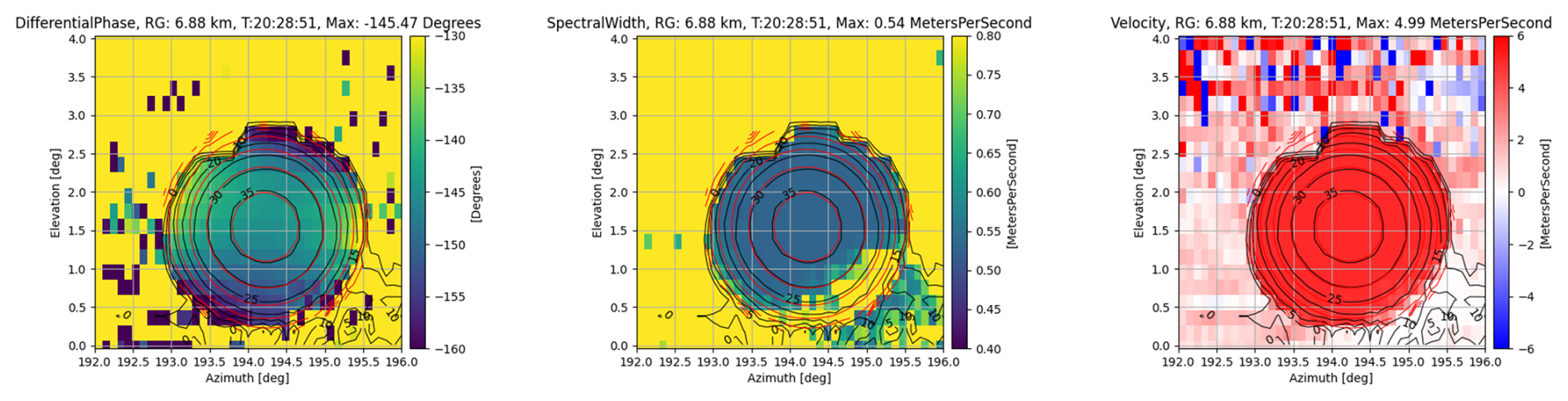
Figure 17 From left to right: box scans of the differential phase Ψ_dp, the Doppler spectrum width σ(v_D), and the Doppler velocity v_D from a target that was scanned with the SPLASH radar and exhibited a Doppler velocity of 4 m s⁻¹.

As expected, the v_D box scan exhibits a homogeneous pattern with a value at the center of the antenna that is very close to the Doppler velocity of the generated target. Towards the lower right corner of the box scan, where reflectivity contamination is increasing, velocities start to degrade from their nominal values. This effect is more prominent in the spectral width data. Ground clutter with spectral components around the zero Doppler line leads to a broadening of the overall spectrum and hence to the increase in σ(v_D) in the lower right corner of the box scan.

The total differential phase Ψ_dp is shown in the first panel of Fig. 17. Neither the RTS nor the radar was corrected for differential phase offsets, and hence only the relative differential phase distribution over the aperture is considered. Antenna differential phase patterns have been measured in Mudukutore et al. (1995), Hubbert et al. (2010), Moisseev et al. (2010), and Myagkov et al. (2015), mainly for assessing the quality of dual-polarization measurements. In general, the authors state that high-quality antennas exhibit lower Ψ_dp variations over the aperture. Within the half-power beam width, Ψ_dp variations on the order of 2° were found for the SPLASH radar, which is qualitatively comparable to the findings in Moisseev et al. (2010) for two C-band radars. A more in-depth analysis of the Ψ_dp distribution is beyond the scope of this article. The respective data are shown solely to illustrate the antenna quality assessment capabilities of measurements based on generated targets.

7 Conclusions

The use of RTS for weather radar calibration offers several advantages, including high precision, repeatability, and flexibility in generating artificial targets with well-defined radar cross-sections (RCSs) and Doppler properties. Unlike static calibration techniques that rely on physical targets such as metal spheres or corner reflectors, RTS facilitates the generation of point targets with controllable parameters, allowing for more robust calibration across a wide range of operational conditions. Additionally, RTS facilitates the evaluation of radar performance without the logistical challenges associated with deploying physical targets.

In evaluating the biases of different radar systems, our experiments highlight key differences in absolute and differential reflectivity calibration, as well as Doppler velocity accuracy. The CHILL radar demonstrates high stability in its reflectivity measurements, with a minimal bias of approximately 0.2 dB over a 1 h time series, indicating excellent calibration performance. Calibration analysis revealed a reflectivity bias of roughly 1.27 dB in the SPLASH radar. Incorporating this adjustment into the data results in well-calibrated reflectivity measurements.

The StXPol radar, on the other hand, showed a significant reflectivity bias in both its long and short pulse channels, with deviations of 5.5 and 4.9 dB, respectively. This offset did not originate from target misplacement but rather from the radar itself. Since the reflectivity bias was inherent in the short and long pulse, persisted over 6 months, was not induced from a target misplacement within the range gate, and also cannot be explained with multipath effects, we are confident that a radar miscalibration is causing this significant discrepancy. Despite this bias, the StXPol radar exhibited high temporal stability, reinforcing confidence in its measurement consistency over time.

For differential reflectivity calibration, the CHILL radar exhibited a considerable bias of −1.43 dB, suggesting the need for further investigation either into system-specific sources of error or possible drawbacks of the experimental setup. In the interpretation of this measured bias it needs to be taken into account that X-band CHILL is a particularly difficult radar to calibrate due to its extremely narrow beam width of 0.3°. In elevation, the generated target was scanned with a resolution of 0.1°, which is most likely sufficient for absolute reflectivity calibration but probably insufficient for Z_dr calibration due to the large variation of this observable within the antenna beam. It is concluded that the scan resolution for accurate Z_dr calibrations should be smaller than a tenth of the antenna's half-power beam width.

The SPLASH radar displayed a Z_dr bias of 0.5 dB, which falls within an acceptable range but still warrants minor corrections for improved accuracy. The StXPol radar performed well in differential reflectivity calibration, with biases of the order of ±0.06 dB for the short and 0.3 dB for the long pulse, indicating high precision in polarimetric measurements.

The RTS also allows one to test the effectiveness of clutter filters by varying the speed of the generated target, making it possible to evaluate the filter response across different Doppler velocities.

A critical factor in achieving accurate reflectivity calibration is the precise placement of the RTS-generated target within the center of the radar's range gate. If the target is positioned at the edge of the range gate, the measured reflectivity can be significantly lower than the expected value, introducing biases as large as 6 dB. Proper target placement is essential to ensuring measurement accuracy across different radar systems.

Additionally, the need for a multipath-free setup is crucial for accurate calibration results. Multipath effects can lead to unwanted signal reflections and distortions, affecting both amplitude and phase measurements. In our experiments, careful placement of the RTS and the use of controlled environments helped to minimize such distortions, leading to more reliable calibration outcomes. The ability to measure the transmit power of the radar provides another layer of validation, as the agreement between the measured and nominal transmit power confirms that the StXPol radar was tested in a multipath-free environment. Because of the importance of conducting measurements without any ground reflections, we plan to conduct upcoming RTS calibrations on a drone platform, which not only improves the calibration accuracy but also enables precise antenna characterization (similar to Segales et al., 2024) and facilitates the experimental setup. Especially for lower-frequency radars like C- or S-band systems, finding clutter-free environments for conducting RTS tests becomes more demanding, since precision horn antennas with the same aperture size as at X-band frequencies exhibit a larger beam width and are hence more prone to receiving ground reflections.

In conclusion, RTS provide an effective solution for weather radar calibration by enabling controlled and repeatable measurements of reflectivity, differential reflectivity, and Doppler velocity. Ensuring proper target placement and minimizing multipath interference are crucial steps in achieving high calibration accuracy. Future improvements in RTS technology and experimental setup refinements will further enhance the precision and reliability of weather radar calibrations.