A relaxed eddy accumulation flask sampling system for ¹⁴C-based partitioning of fossil and non-fossil CO₂ fluxes

A relaxed eddy accumulation (REA) system was developed and tested, enabling conditional sampling of air for subsequent ¹⁴CO₂ analysis. This allows a ¹⁴C-based estimation of fossil fuel CO₂ concentrations in the collected air samples and, thus, an observation-based partitioning of total CO₂ fluxes measured in urban environments by eddy covariance into fossil and non-fossil components. This article describes the REA system, evaluates its performance, and assesses uncertainties in the concentration measurements. In the REA system, two separate inlet lines equipped with fast-response valves and loop systems adapted to the technical requirements enable the conditional collection of air in two sets of aluminum cylinders for updraft and downdraft samples, respectively. The switching between updraft sampling, downdraft sampling, and standby mode is thereby determined by the vertical wind measured at 20 Hz by a co-located ultrasonic 3D anemometer. A logger program provides different options for the definition of a deadband, which is used to increase the concentration differences between updraft and downdraft samples. After the sampling interval, the accumulated air is transferred by an automated 24-port flask sampler into 3 L glass flasks, which can be analyzed in the laboratory, and the cylinders are re-evacuated for the next sampling. The REA system was tested in the laboratory, as well as on a tall tower near the city center of Zurich, Switzerland. Between July 2022 and April 2023, 103 REA updraft and downdraft flask pairs for flux measurements and 9 flask pairs for quality control purposes were selected from the tall tower for laboratory analysis based on suitable micro-meteorological conditions. Uncertainties in the CO₂ concentration differences between updraft and downdraft flasks were estimated by simulations using 20 Hz in situ measurements of a closed-path gas analyzer and an open-path gas analyzer co-located with the ultrasonic anemometer. The measurements show that there is no significant bias in the concentration differences between updraft and downdraft samples and that uncertainties due to the sampling process are negligible when estimating fossil fuel CO₂ signals. In the Zurich measurements, the CO₂ concentration differences between the flask pairs agreed with the differences obtained from in situ measurements within −0.005 ± 0.227 ppm. The largest source of uncertainty, as well as the main limitation, in the separation of fossil and non-fossil CO₂ signals in Zurich was the small signal-to-noise ratio of the Δ¹⁴C differences measured by accelerator mass spectrometry between the updraft and downdraft flasks. The novel REA flask sampling system meets the high technical requirements of the REA method and is a promising technology for observation-based estimation of fossil fuel CO₂ fluxes.

1 Introduction

In view of the overarching aim of reducing anthropogenic greenhouse gas emissions to mitigate climate change, reliable emissions data and timely information on emission reductions are indispensable, especially at the local scale in urban environments where emission reduction efforts are to be assessed. Of central importance in this context is the quantification of fossil fuel CO₂ (ffCO₂) emissions in cities as cities contribute more than 70 % to global and European ffCO₂ emissions (Seto et al., 2014). Officially reported bottom-up emission inventories are usually based on statistical activity data, e.g., fossil fuel consumption, and emission factors for the different emission sectors, such as traffic or industry (Super et al., 2020). Downscaled to urban and local resolutions, they form an important basis for policy decisions, as well as for fundamental research (WMO, 2022). Despite continuous improvements to such inventories, the benefits of bottom-up estimates are currently limited by their coarse spatial and temporal resolutions, large uncertainties in the available methodologies, and the delayed availability of data (Gately and Hutyra, 2017; Lauvaux et al., 2020; Stagakis et al., 2023). To independently validate and refine emission inventories for CO₂, atmospheric measurements providing timely, localized, and sector-specific top-down information are therefore indispensable.

The only method that allows direct measurement of vertical atmospheric trace gas fluxes is the eddy covariance (EC) technique, in which vertical wind velocity and trace gas concentrations are both measured at a frequency of 10 to 20 Hz (e.g., Mauder et al., 2021). Although this method assumes a horizontally flat and homogeneous surface area (Foken et al., 2012), studies have shown that EC measurements can also be successfully performed in a complex and heterogeneous urban environment (Grimmond and Christen, 2012; Feigenwinter et al., 2012; Christen, 2014). However, EC-based CO₂ flux estimates contain fossil and non-fossil components. Models and measurements have shown that biospheric CO₂ fluxes (autotrophic and heterotrophic respiration and photosynthesis) can contribute significantly to the total CO₂ flux measured over an urban area, even in winter (e.g., Crawford et al., 2011; Kellett et al., 2013; Hardiman et al., 2017; Wu et al., 2022). In addition, human respiration fluxes typically account for about 5 % of the total annual CO₂ flux, depending on the population and emission density (e.g., Kellett et al., 2013; Crawford and Christen, 2015). Considering the increasing use of biofuels as well (e.g., Guo et al., 2015), this results in significant uncertainties in inverse estimates of fossil fuel emissions (Crawford and Christen, 2015; Wu et al., 2018; Stagakis et al., 2023).

In separating fossil and non-fossil CO₂ enhancements, radiocarbon has proven to be the ideal tracer since ¹⁴C-free fossil fuels dilute the atmospheric ${}^{\mathrm{14}}\mathrm{C}/\mathrm{C}$ ratio compared to a clean background (e.g., Levin et al., 2003; Turnbull et al., 2016). To measure the atmospheric ${}^{\mathrm{14}}\mathrm{C}/\mathrm{C}$ ratio (on the order of 10⁻¹²), air is commonly sampled in glass flasks and subsequently analyzed in the laboratory, e.g., by accelerator mass spectrometry of the extracted and catalytically reduced CO₂ (Lux, 2018). Based on long-term atmospheric ¹⁴CO₂ observations, Levin et al. (2003) quantified the ffCO₂ enhancements at three German sites and used the radon tracer method to derive ffCO₂ fluxes for the respective catchment areas. Maier et al. (2024a) analyzed the ratio of carbon monoxide (CO), which is co-emitted with ffCO₂, to get a continuous time series of the excess ffCO₂ concentration in Heidelberg, Germany, and used an atmospheric inversion model to obtain ffCO₂ fluxes (Maier et al., 2024b). Wu et al. (2022) used the mean ΔCO $/$ ΔffCO₂ ratio of flask pairs collected at two towers in Indianapolis, USA, to derive ffCO₂ fluxes from CO fluxes measured by the flux gradient approach. However, to derive ffCO₂ fluxes, all methods rely on the assumption of constant proxy $/$ ffCO₂ ratios or results from inversion models. Direct ¹⁴C-based ffCO₂ flux measurements have not been possible so far because the precision and temporal resolution of state-of-the-art lasers for ¹⁴C in situ measurements are still far too low for EC measurements (e.g.,  Lehmuskoski et al., 2021; McCartt and Jiang, 2022). The relaxed eddy accumulation (REA) method (Businger and Oncley, 1990), on the other hand, allows for flux estimation from the concentration differences between two conditionally collected air samples, which can be determined in the laboratory. The ffCO₂ fluxes can thus be estimated from the ¹⁴C-based ffCO₂ concentration differences between updraft and downdraft flask sample pairs.

In the present study, to our knowledge, the first REA system for ¹⁴C-based estimation of ffCO₂ fluxes was developed. Based on the principles of relaxed eddy accumulation (Sect. 2) and ¹⁴C-based fossil fuel CO₂ estimation (Sect. 3), the purpose of this article is to describe the novel REA flask sampling system (Sect. 4), as well as to evaluate its performance and assess the uncertainties of the concentration measurements (Sect. 5). As a proof of concept of the ¹⁴C-based separation of fossil and non-fossil CO₂ components, the ffCO₂ concentration differences between updraft and downdraft flasks collected during a field campaign at a tall tower 112 m above ground level near the city center of Zurich, Switzerland, are presented (Sect. 6). This work forms the basis for the derivation and analysis of ffCO₂ fluxes in Zurich and for future deployments in other urban environments.

2 The relaxed eddy accumulation method

Relaxed eddy accumulation (REA), first described by Businger and Oncley (1990), is a conditional sampling method for measuring turbulent trace gas fluxes using slow-response analyzers. A fast ultrasonic anemometer measures the vertical wind velocity w at a frequency of 10 to 20 Hz. Based on w, the opening and closing of two fast-response sampling valves are controlled in quasi-real time. Any bias in the vertical wind velocity must therefore be removed before activating the valves (Rinne et al., 2021). When there is an updraft eddy and w is above a certain threshold w₀, air is collected and accumulated in an updraft reservoir, whereas air is collected in a separate downdraft reservoir when w < −w₀.

The range of wind speeds $[-w_{\mathrm{0}}:w_{\mathrm{0}}]$ where no air is collected is called the deadband. Under ideal conditions, the mean vertical wind speed $\stackrel{\mathrm{‾}}{w}$ over a sampling period of, for example, 30 or 60 min is zero and defines the center of the deadband. The deadband width can be constant or dynamically adjusted in relation to the standard deviation of the vertical wind speed σ_w so that w₀ = $\stackrel{\mathrm{‾}}{w}+\mathit{\delta }{\mathit{\sigma }}_{\mathrm{w}}$ (Rinne et al., 2021). The larger the δ, the greater the concentration difference between the updraft and downdraft reservoirs, reducing the relative measurement uncertainty (Rinne et al., 2021). In addition, a larger deadband reduces the switching frequency of the sampling valves, thereby increasing their lifetime (Rinne et al., 2021). However, this also reduces the fraction of time during which air is collected, which reduces the sample volume and the statistical significance. A compromise between a high concentration difference, a sufficient sample volume, and good representativity has to be found (Christen et al., 2006). Since the requirement $\stackrel{\mathrm{‾}}{w}$ = 0 can be violated, particularly in urban environments with complex airflow, and since the actual value of $\stackrel{\mathrm{‾}}{w}$ is not known before the end of the sampling period, two options to trigger the valves based on vertical wind were implemented in this study (see Sect. 4.1).

The flow rate into the two reservoirs is always zero when the valves are closed and constant when they are open. This relaxes the high technical requirements of the true eddy accumulation method proposed by Desjardins (1972), where the sampling rate is adjusted in quasi-real time in relation to the magnitude of the vertical wind velocity (for a detailed description, see Siebicke and Emad, 2019, and Emad and Siebicke, 2023). However, the constant flow rate prevents a direct assessment of the mean vertical turbulent flux of a trace gas F_c. With REA, F_c is calculated according to Eq. (1) from the mean concentration difference between the updraft and the downdraft sample Δc, the standard deviation of the vertical wind speed σ_w, the mean molar air density $\stackrel{\mathrm{‾}}{{\mathit{\rho }}_{\mathrm{m}}}$, and an empirical coefficient β.

$$\begin{array}{}\text{(1)}& F_{\mathrm{c}}=\mathit{\beta }{\mathit{\sigma }}_{\mathrm{w}}\stackrel{\mathrm{‾}}{{\mathit{\rho }}_{\mathrm{m}}}\left(c^{\uparrow }-c^{\downarrow }\right)=\mathit{\beta }{\mathit{\sigma }}_{\mathrm{w}}\stackrel{\mathrm{‾}}{{\mathit{\rho }}_{\mathrm{m}}}\mathrm{\Delta }c\end{array}$$

The proportionality factor β depends on the joint probability distribution of variations in the vertical wind velocity and the trace gas concentration (Milne et al., 1999). Without a deadband and under an ideal joint Gaussian distribution of w and c, β is 0.627 (Wyngaard, 1992; Baker et al., 1992), but the dependence of β on the prevailing atmospheric conditions; the deadband width; and, eventually, the scalar, e.g., the trace gas concentration, itself adds uncertainty into the calculated flux (Siebicke and Emad, 2019). Grönholm et al. (2008) showed that, with a deadband dynamically adjusted based on the standard deviation of the vertical wind velocity, β does not depend on the atmospheric stability, allowing the use of a constant value in flux calculations. Consequently, assuming similarity in the turbulent exchange of two quantities, β can be determined with Eq. (1) from a scalar where the flux is known from EC measurements, e.g., temperature or CO₂ (Rinne et al., 2021).

Estimating the ffCO₂ difference between updraft and downdraft reservoirs based on ¹⁴CO₂ analyses of REA sample pairs and assuming scalar similarity between CO₂ and ¹⁴CO₂, Eq. (1) allows us to determine the fossil contribution to a total CO₂ flux:

$$\begin{array}{}\text{(2)}& {\displaystyle \frac{F_{{\mathrm{ffCO}}_{\mathrm{2}}}}{F_{{\mathrm{CO}}_{\mathrm{2}}}}}={\displaystyle \frac{\mathrm{\Delta }{\mathrm{ffCO}}_{\mathrm{2}}}{\mathrm{\Delta }{\mathrm{CO}}_{\mathrm{2}}}}.\end{array}$$

In this paper, only the concentration differences (right-hand side of Eq. 2) and their uncertainties are analyzed. The observation-based ffCO₂ fluxes, which can be obtained by multiplying the $\mathrm{\Delta }{\mathrm{ffCO}}_{\mathrm{2}}/\mathrm{\Delta }{\mathrm{CO}}_{\mathrm{2}}$ ratio of the REA samples with $F_{{\mathrm{CO}}_{\mathrm{2}}}$ from EC measurements, will be presented in a follow-up work.

It should be noted that Eq. (2) is unstable for $F_{{\mathrm{CO}}_{\mathrm{2}}}$ and/or ΔCO₂ close to zero. In this case, a proxy other than CO₂ is needed, e.g., CO. Moreover, like any other method based on the eddy covariance principle, REA only provides reasonable estimates of the mean vertical turbulent flux if the micro-meteorological conditions are stationary and if turbulence is well developed during the sampling period (Foken et al., 2012). If a temporal change in concentrations below the measurement height causes a significant storage flux, the measured turbulent fluxes are not representative of the respective surface fluxes at the time (Crawford and Christen, 2014; Bjorkegren et al., 2015). Further, if vertical advection leads to significant flux components due to non-turbulent vertical transport, this cannot be properly captured by eddy covariance and the REA approach (Foken et al., 2012). This implies the consideration of various criteria when selecting suitable samples in any application (see Sect. 4.4).

3 ¹⁴C-based fossil fuel CO₂ estimation

In determining the contribution of fossil fuel emissions to a measured CO₂ signal, ¹⁴C has turned out to be an important tracer. The radioactive carbon isotope has a half-life of 5730 years. Consequently, the millions-of-years-old fossil fuels are ¹⁴C-free; hence, CO₂ emitted by fossil fuel combustion (ffCO₂) dilutes the atmospheric ${}^{\mathrm{14}}\mathrm{C}/\mathrm{C}$ ratio. Due to the low ¹⁴C abundance, the specific activity of a reservoir or sample is commonly given as the relative deviation (in ‰) from the absolute specific activity of the radiocarbon standard A_ABS = 0.2261 Bq gC⁻¹ (Eq. 3) (Stuiver and Polach, 1977). This is commonly denoted as Δ¹⁴C but is abbreviated to Δ¹⁴ in this work to improve the readability of the following equations.

$$\begin{array}{}\text{(3)}& {\mathrm{\Delta }}^{\mathrm{14}}=\left({\displaystyle \frac{A_{\mathrm{SN}}}{A_{\mathrm{ABS}}}}-\mathrm{1}\right)\times \mathrm{1000}\end{array}$$

A_SN is the ¹⁴C sample activity A_S normalized to the postulated mean δ¹³C value of terrestrial wood of −25 ‰ to correct for isotopic fractionation due to biological or physical processes during the sample formation and the measurement routine (Stuiver and Polach, 1977):

$$\begin{array}{}\text{(4)}& A_{\mathrm{SN}}=A_{\mathrm{S}}\left(\mathrm{1}-{\displaystyle \frac{\mathrm{2}\left(\mathrm{25}+\mathit{\delta }{}^{\mathrm{13}}\mathrm{C}\right)}{\mathrm{1000}}}\right).\end{array}$$

Following the general approach of Turnbull et al. (2016) and Maier et al. (2023), any measured atmospheric ¹⁴CO₂ signal can, analogously to the total CO₂ concentration c_meas, be expressed as the sum of a background (bg), a fossil fuel (ff), a biofuel (bf), a nuclear (nuc), a stratospheric (strato), a respiratory (resp), a photosynthetic (photo), and an oceanic (oc) component:

$$\begin{array}{}\text{(5)}& {\displaystyle }{c}_{\mathrm{meas}}=\sum _i{c}_i,\text{(6)}& {\displaystyle }\begin{array}{l}{c}_{\mathrm{meas}}\mathrm{\Delta }{}^{\mathrm{14}}=\sum _i{c}_i{\mathrm{\Delta }}_i^{\mathrm{14}},\\ i=\text{bg, ff, bf, nuc, strato, resp, photo, oc}.\end{array}\end{array}$$

On a local scale, as during REA sampling, it can be assumed that two air parcels differ only in terms of their fossil fuel, biofuel, respiration, and photosynthesis components, while the impact of the other, more distant sinks and sources is the same. Since biofuels and respiration have a similar Δ¹⁴ signature, they cannot be distinguished by radiocarbon analysis alone and are therefore summarized in the following as non-fossil (nf) CO₂ emissions, with respiration being by far the largest contributor. Thus, the concentration differences between the updraft (↑) and the downdraft (↓) reservoir of an REA measurement can be expressed in the following way:

$$\begin{array}{}\text{(7)}& {\displaystyle }{c}_{\mathrm{meas}}^{\uparrow }-c_{\mathrm{meas}}^{\downarrow }=\left(c_{\mathrm{ff}}^{\uparrow }-c_{\mathrm{ff}}^{\downarrow }\right)+\left(c_{\mathrm{nf}}^{\uparrow }-c_{\mathrm{nf}}^{\downarrow }\right)+\left(c_{\mathrm{photo}}^{\uparrow }-c_{\mathrm{photo}}^{\downarrow }\right),\text{(8)}& {\displaystyle }\begin{array}{rl}& c_{\mathrm{meas}}^{\uparrow }{{\mathrm{\Delta }}_{\mathrm{meas}}^{\mathrm{14}}}^{\uparrow }-c_{\mathrm{meas}}^{\downarrow }{{\mathrm{\Delta }}_{\mathrm{meas}}^{\mathrm{14}}}^{\downarrow }=\left(c_{\mathrm{ff}}^{\uparrow }-c_{\mathrm{ff}}^{\downarrow }\right)\cdot {\mathrm{\Delta }}_{\mathrm{ff}}^{\mathrm{14}}\\ & +\left(c_{\mathrm{nf}}^{\uparrow }-c_{\mathrm{nf}}^{\downarrow }\right)\cdot {\mathrm{\Delta }}_{\mathrm{nf}}^{\mathrm{14}}+\left(c_{\mathrm{photo}}^{\uparrow }-c_{\mathrm{photo}}^{\downarrow }\right)\cdot {\mathrm{\Delta }}_{\mathrm{photo}}^{\mathrm{14}}.\end{array}\end{array}$$

Combining Eq. (7) and Eq. (8), the difference in c_ff between updraft and downdraft reservoirs can be estimated via

$$\begin{array}{}\text{(9)}& \begin{array}{rl}& c_{\mathrm{ff}}^{\uparrow }-c_{\mathrm{ff}}^{\downarrow }={\displaystyle \frac{\mathrm{1}}{{\mathrm{\Delta }}_{\mathrm{photo}}^{\mathrm{14}}-{\mathrm{\Delta }}_{\mathrm{ff}}^{\mathrm{14}}}}\left[c_{\mathrm{meas}}^{\uparrow }\right({\mathrm{\Delta }}_{\mathrm{photo}}^{\mathrm{14}}-{{\mathrm{\Delta }}_{\mathrm{meas}}^{\mathrm{14}}}^{\uparrow })\\ & -c_{\mathrm{meas}}^{\downarrow }({\mathrm{\Delta }}_{\mathrm{photo}}^{\mathrm{14}}-{{\mathrm{\Delta }}_{\mathrm{meas}}^{\mathrm{14}}}^{\downarrow })+(c_{\mathrm{nf}}^{\uparrow }-c_{\mathrm{nf}}^{\downarrow })({\mathrm{\Delta }}_{\mathrm{nf}}^{\mathrm{14}}-{\mathrm{\Delta }}_{\mathrm{photo}}^{\mathrm{14}})].\end{array}\end{array}$$

The corresponding uncertainty is derived according to Gauss' law of error propagation.

Since fossil fuel emissions do not contain any ¹⁴C, ${\mathrm{\Delta }}_{\mathrm{ff}}^{\mathrm{14}}$ is, by definition, exactly −1000 ‰. On the contrary, biogenic signatures are heterogeneous and much more uncertain (e.g., Naegler and Levin, 2009b; Maier et al., 2023). To estimate $c_{\mathrm{ff}}^{\uparrow }-c_{\mathrm{ff}}^{\downarrow }$ (in the following denoted as ΔffCO₂), it is therefore necessary to make assumptions about ${\mathrm{\Delta }}_{\mathrm{photo}}^{\mathrm{14}}$, ${\mathrm{\Delta }}_{\mathrm{nf}}^{\mathrm{14}}$ and $c_{\mathrm{nf}}^{\uparrow }-c_{\mathrm{nf}}^{\downarrow }$.

Since the Δ notation accounts for mass-dependent isotopic fractionation (Eq. 4), ${\mathrm{\Delta }}_{\mathrm{photo}}^{\mathrm{14}}$ corresponds to the ¹⁴C signature of the photosynthesized atmospheric CO₂. For our measurements of local CO₂ fluxes close to the tall tower, ${\mathrm{\Delta }}_{\mathrm{photo}}^{\mathrm{14}}$ is therefore best approximated by the measured atmospheric signature ${\mathrm{\Delta }}_{\mathrm{meas}}^{\mathrm{14}}$. As there are always two flasks per REA run, the average of the up and down flasks is chosen: ${\mathrm{\Delta }}_{\mathrm{photo}}^{\mathrm{14}}\approx \mathrm{0.5}\cdot ({{\mathrm{\Delta }}_{\mathrm{meas}}^{\mathrm{14}}}^{\uparrow }+{{\mathrm{\Delta }}_{\mathrm{meas}}^{\mathrm{14}}}^{\downarrow }$). However, due to temporal variability, the ${\mathrm{\Delta }}_{\mathrm{photo}}^{\mathrm{14}}$ uncertainty is larger than the measurement uncertainty (∼ 1.8 ‰; see Appendix D) and is therefore set to 10 ‰.

Non-fossil CO₂ (from autotrophic and heterotrophic respiration and, to a lesser extent, biofuels) is generally more enriched in ¹⁴CO₂ because heterotrophically respired CO₂ and CO₂ from biofuels were taken up by the biosphere several years to decades ago. At that time, the atmospheric Δ¹⁴ was higher due to ¹⁴CO₂ released during nuclear bomb tests in the 1950s–1960s, which constituted the dominant contribution up to the 2000s (Naegler and Levin, 2009a). Since then, the strongest component of the ongoing atmospheric Δ¹⁴ decline has been the emission of fossil fuel CO₂ (Levin et al., 2010; Turnbull et al., 2016). In total, the Δ¹⁴ signature of respiration was found to be larger than atmospheric values by a few tens of permil (e.g., Palonen et al., 2018; Chanca, 2022). Following Maier et al. (2023), an enrichment of the respiration-dominated ${\mathrm{\Delta }}_{\mathrm{nf}}^{\mathrm{14}}$ of 25 ± 12 ‰ is assumed in this study. The atmospheric signature during CO₂ uptake of the biospheric $\stackrel{\mathrm{‾}}{{\mathrm{\Delta }}_{\mathrm{atmo}}^{\mathrm{14}}}$ is estimated by the mean ${\mathrm{\Delta }}_{\mathrm{meas}}^{\mathrm{14}}$ value in summer, when photosynthesis is most pronounced.

The third unknown is the difference Δc_nf = $c_{\mathrm{nf}}^{\uparrow }-c_{\mathrm{nf}}^{\downarrow }$. This can be estimated based on the mean measured total CO₂ differences between up and down flasks and the assumption that, in an urban setting, there is always a fossil contribution. Since this is only a very rough and upper estimate, a relative uncertainty of 100 % is reasonable.

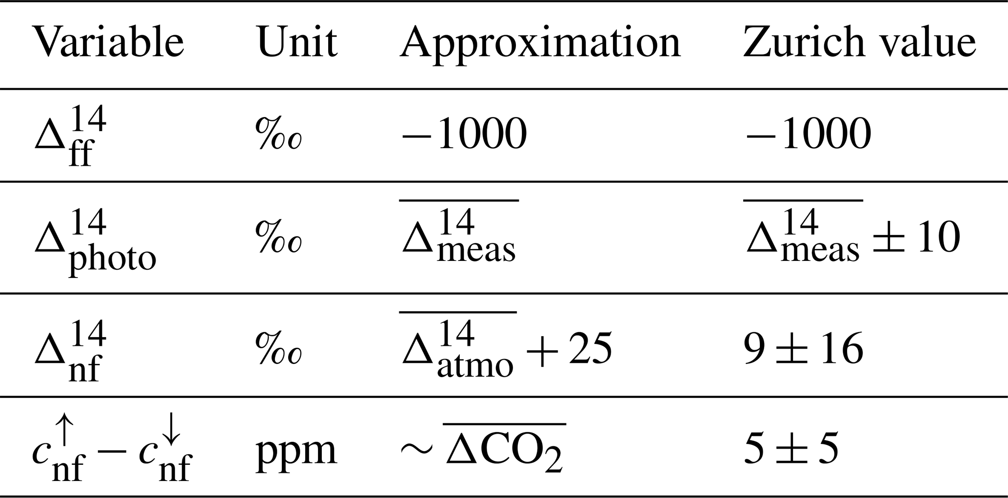
The assumptions regarding ${\mathrm{\Delta }}_{\mathrm{photo}}^{\mathrm{14}}$, ${\mathrm{\Delta }}_{\mathrm{nf}}^{\mathrm{14}}$, and Δc_nf, as well as the specific values used to calculate ΔffCO₂ from the REA flasks of the first measurement campaign in Zurich, are summarized in Table 1. Although ${\mathrm{\Delta }}_{\mathrm{photo}}^{\mathrm{14}}$, ${\mathrm{\Delta }}_{\mathrm{nf}}^{\mathrm{14}}$, and Δc_nf are not well known, the uncertainty in the ΔffCO₂ estimates is dominated by the ¹⁴CO₂ measurement uncertainty, which currently leads to an inherent ΔffCO₂ uncertainty of 0.7 ppm at least and 1.2 ppm on average. Details are given in Appendix D.

Table 1 Variables used to estimate $c_{\mathrm{ff}}^{\uparrow }-c_{\mathrm{ff}}^{\downarrow }$ = ΔffCO₂. ${\mathrm{\Delta }}_i^{\mathrm{14}}$ denotes the Δ¹⁴ values of fossil fuels (ff), photosynthetic (photo) and non-fossil (nf) CO₂, and flask measurements (meas). $\stackrel{\mathrm{‾}}{{\mathrm{\Delta }}_{\mathrm{meas}}^{\mathrm{14}}}$ = $\mathrm{0.5}\cdot ({{\mathrm{\Delta }}_{\mathrm{meas}}^{\mathrm{14}}}^{\uparrow }+{{\mathrm{\Delta }}_{\mathrm{meas}}^{\mathrm{14}}}^{\downarrow })$ denotes the mean of the updraft and downdraft samples, which is different for each REA run. The atmospheric signature during CO₂ uptake of the biosphere $\stackrel{\mathrm{‾}}{{\mathrm{\Delta }}_{\mathrm{atmo}}^{\mathrm{14}}}$ is estimated by the mean ${\mathrm{\Delta }}_{\mathrm{meas}}^{\mathrm{14}}$ value in summer (July to September 2022 in the case of the Zurich campaign). Also given are the specific values derived for the first measurement campaign in Zurich.

4 Setup of the REA system

The relaxed eddy accumulation (REA) flask sampling system consists of an eddy covariance (EC) system with a 3D ultrasonic anemometer and an integrated open-path gas analyzer (IRGASON, Campbell Scientific Inc., Logan, UT, USA); two fast-response valves controlled by a solid-state DC control module (SDM-CD8S, Campbell Scientific Inc., Logan, UT, USA); a data logger (CR6, Campbell Scientific Inc., Logan, UT, USA); and an extension of a regular 24-port ICOS (Integrated Carbon Observation System) automated flask sampler, described, for example, in Levin et al. (2020) (Fig. 1). This allows the collection of updraft and downdraft air samples (Sect. 2) in glass flasks for subsequent laboratory analysis.

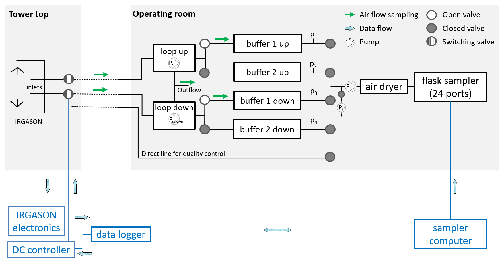
Figure 1 Schematic setup of the REA flask sampling system. P_a–P_c refers to the pumps that transfer the air from the inlets to the flask sampler and evacuate the buffers after sample transfer. p₁–p₄ indicates pressure sensors. Blue components at the bottom of the diagram depict the general wiring for data transfer and communication between the data logger and the sampler computer. The green arrows and the filled, unfilled, and hatched circles indicate the air flow and the position of the valves when sampling for buffer set 1. Details of the loop systems are shown in Fig. 2.

As depicted in Fig. 1, there are two inlets, one for updraft conditions and one for downdraft conditions. They are about 20 cm away from the center of the ultrasonic anemometer and are horizontally separated from each other by about 5 cm. The collection of air is controlled by the two solenoid valves located approximately 30 cm behind the inlets. They respond to the data logger's 20 Hz signal, which is based on the vertical wind velocity measurements of the IRGASON (Sect. 4.1). This signal is also sent to the sampler computer, which controls the extended flask sampler. Two pumps (P_a, up and P_a, down in Fig. 1) transfer the sampled air into two separate 50 L cylinders, which are called buffers in the following. The so-called loop systems (Sect. 4.2) avoid flow rate fluctuations during sampling and non-sampling to ensure constant flow rates despite high-frequency switching. Excess air from the updraft and downdraft sides is released through one common outflow. After a successful sampling event, for which both 50 L buffers need to have a pressure between 1.2 and 1.6 bar (Sect. 4.3), the samples are dried and transferred into 3 L glass flasks (pump P_b), and the buffers are evacuated again (pump P_c). Since this takes about 45 min, there is a second pair of buffers that can be filled in the meantime. This allows for a nearly continuous sampling routine. The flask pairs can be sent to the laboratory or re-sampled if, for example, the sampling conditions did not fulfill the requirements (Sect. 4.4). In addition, a third line from the tower top directly to the flask sampler enables a simultaneous sampling of flasks with a regular $\mathrm{1}/t$ filling (Levin et al., 2020), which can be used for quality control tests (Sect. 5.3.1). In the following, the individual steps of collecting REA flasks are described in more detail. The following terminology is used: REA run denotes the REA sampling event of usually 1 h; REA ID denotes the unique, consecutively assigned number for each REA run; sampling mode denotes the state of the updraft or downdraft line when air is collected, i.e, when the vertical wind is above or below the deadband; and standby mode denotes the state of the updraft or downdraft line when no air is collected, i.e, when the vertical wind is below or above or within the deadband. A photo of the inlets and the extended flask sampler and specifications of the components of the system are shown in Fig. 3 and Appendix A.

4.1 Conditional collection of air

During an REA run, the data logger controls the opening and closing of the solenoid valves at the inlets according to the in situ measurements of the vertical wind velocity. Depending on the definition of the deadband (Sect. 2), flags are assigned to each 20 Hz wind measurement, denoting the status of the two valves in the current and previous time step. If the two values are different, the corresponding valve is switched. For quality control, the flags, called REA flags in the following, can be used to estimate the sample CO₂ concentrations from high-frequency in situ concentration measurements (see Sect. 5.2 and 5.3.2).

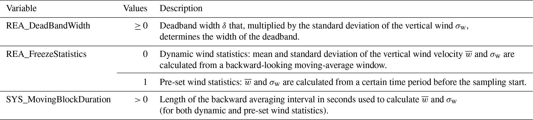
Table 2 shows the possible deadband settings implemented in the logger program, which can be selected depending on the scientific question and site-specific requirements.

Table 2 Variables in the logger program that determine the deadband of the REA run.

It should be noted that the digital output from the IRGASON is delayed by several hundred milliseconds depending on the bandwidth of the low-pass filter that is applied to the actual 60 Hz measurements. The larger the bandwidth, the smaller the delay, with a minimum delay of 200 ms (20 Hz bandwidth). In addition, there will also be a short delay between the signals being sent, the valves being physically switched, and the air being sucked in due to the slight underpressure in the line. The impact of these delays on the flask concentration differences is analyzed in Sect. 5.2.1.

4.2 Transfer of collected air into buffers

To pump the collected air at a constant flow rate into the respective buffers while ensuring that the system can switch between sampling and standby mode at any time, loop systems (Fig. 2) were developed. They consist of a membrane pump that runs continuously, a pressure control valve, a mass flow controller (MFC), and two three-way valves. The technical details of the components are given in Appendix A.

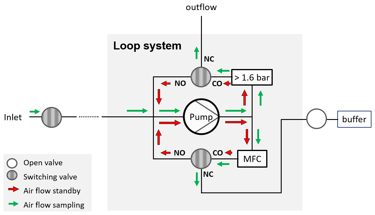
Figure 2 Schematic setup of the loop systems indicating the air flow in sampling and standby mode. NC: normally closed (closed in standby mode, open in sampling mode); NO: normally open (open in standby mode, closed in sampling mode); CO: constantly open; MFC: mass flow controller; > 1.6 bar: pressure control valve.

When the solenoid valve at the inlet is closed (i.e., in standby mode when no air is sampled), the three-way valves are closed to the outside, causing the air to circulate in two loops. As shown by the red arrows, the air splits behind the pump: one part flows through the MFC and the constantly open (CO) and normally open (NO) positions of the three-way valve connected to the buffer, while the other part flows through the pressure control valve and the second three-way valve until both reach the suction side of the pump again. The air in the intake line between the inlet and the pump does not move. In sampling mode, both three-way valves switch to the normally closed (NC) position. Then, air is pumped through the line and the MFC into the buffer, while excess air leaves the system through the pressure control valve, as indicated by the green arrows. In both modes, the pump is continuously running, and the pressure behind the pump and the flow rate through the loop are constant due to the pressure control valve and the MFC. Thus, in sampling mode, the flow rate into the buffers is approximately constant, and the system is able to switch between sampling and standby mode at any time. The effect of a remaining variability in the flow rates is discussed in Sect. 5.2.3.

Each loop system has an internal volume of V_l = 12.0 ± 1.1 mL, while the volumes of the inlet tubes with length l_t and radius r_t are V_t = $\mathit{\pi }{r}_{\mathrm{t}}^{\mathrm{2}}{l}_{\mathrm{t}}$. The pump flow velocity q_pump (L min⁻¹) depends on the dimensions of the intake lines (longer and thinner tubes have a higher resistance) and the flow rate set at the MFC. The latter is adjusted based on the length of the REA run and the deadband width δ: the shorter the REA run and the larger the deadband width, the larger the required flow rate into the buffers. Consequently, an air parcel needs the time

$$\begin{array}{}\text{(10)}& t_{\mathrm{r}}=\left(V_{\mathrm{l}}+V_{\mathrm{t}}\right)/q_{\mathrm{pump}}\end{array}$$

from the inlet to the buffer. We refer to t_r as the “rinse time” in the following because it is the exact amount of time by which sampling needs to be delayed artificially in order to avoid sampling air from before the event. For this purpose, the valves at the buffers remain closed for the first t_r seconds in sampling mode so that the residual air is released through the outflow. On the contrary, the pump stays on, and all valves remain open for an additional t_r seconds after the end of the sampling period so that all sample air remaining in the tubes is transferred into the buffers. Due to the site-specific lengths of the intake lines, t_r must be individually calculated and adjusted in the sampler software. As shown in Sect. 5.1 and 5.2.2, calculated values agree well with measurements of the travel time of a CO₂ pulse, and uncertainties in the flask concentrations resulting from the uncertainty of t_r are negligible.

4.3 Transfer of accumulated air into glass flasks

After the sampling period, the accumulated air is transferred from the buffers into 3 L glass flasks in the flask sampler. Thereby, it is dried to a dew point of approximately −40 °C. To (almost) completely replace the initial air content of a flask with the sample air from the buffers, the flask volume is flushed 10 times at atmospheric pressure. Then the flask is filled up to 2 bar. As the performance of the sampler transfer pump does not allow us to use the entire sample volume in the buffers, a minimal sample amount of 60 L is desired, corresponding to a pressure of 1.2 bar in the buffers. Excess air is discarded when the buffers are evacuated. At the same time, the maximum pressure at which the pumps in the loop systems can be operated is 1.6 bar, and so an REA run is automatically stopped when either buffer reaches this threshold. Consequently, an REA sampling event is only successful if the pressures of the updraft and downdraft buffers are between 1.2 and 1.6 bar at the end of sampling.

4.4 Sample selection for laboratory analysis

The REA flasks are analyzed with gas chromatography for CO₂, CO, CH₄, N₂O, SF₆, and H₂ at the ICOS Flask and Calibration Laboratory (FCL) in Jena, Germany. To measure ¹⁴CO₂, the flasks are sent to the ICOS Central Radiocarbon Laboratory (CRL) in Heidelberg. There, the CO₂ is extracted from the remaining air sample and catalytically reduced to graphite (Lux, 2018). The graphite targets are then analyzed for the ${}^{\mathrm{14}}\mathrm{C}/\mathrm{C}$ ratio with an accelerator mass spectrometer at the Curt-Engelhorn-Centre Archaeometry in Mannheim, Germany. Since the measurement process is complex and because funding is limited, a thorough selection of appropriate samples is necessary. Several criteria are important to consider.

First, it must be ensured that there were no technical problems with the IRGASON or the flask sampler, i.e., that the CO₂ signal strength of the IRGASON was above 90 %, that the valves were switching, that the flow rate into the buffers was approximately constant, and that the horizontal wind direction was not from sectors with known flow distortion effects of the ultrasonic anemometer or the tower structure. Second, the assumptions made in the EC and REA methods, namely stationarity and well-developed turbulence (Sect. 2), must have been fulfilled during the sampling period. For this purpose, the 20 Hz measurements of the IRGASON during the sampling period can be analyzed. In this study, the software EddyPro (version 7.0.9, Licor Inc., Lincoln, NE, USA) was used to process the data. Flask samples were discarded if the integral turbulence characteristic test for w (Foken et al., 2004) was greater than 100 % and if the steady-state test for the covariance between the vertical wind w and the CO₂ concentration (Foken et al., 2004) was greater than 400 %.

Depending on the aim of the application, further selection criteria may be considered in the selection of REA flasks. If the objective is a ¹⁴C-based decomposition of total CO₂ surface fluxes, the fossil fuel CO₂ differences between updraft and downdraft samples should be greater than the inherent measurement uncertainty of 0.7 ppm that is caused by the current ¹⁴CO₂ measurement precision (see Appendix D). For times during which photosynthesis is expected to be weak, estimates of total ΔCO₂ based on the IRGASON measurements are good indicators.

4.5 Zurich installation

The REA system was installed and operated for the first time in Zurich, Switzerland, from July 2022 to April 2023. The IRGASON and REA inlets were mounted on a radio tower of 16.5 m height on top of a 95.3 m tall high-rise residential building (Fig. 3). The data loggers, the network devices, and the REA flask sampler were placed in a climate-controlled room on the top floor of the building. The building is surrounded by an industrial sector, railway lines, and a busy commuting road to the north; an urban sector (city center) to the southeast; and a green, less densely populated area with a cemetery to the southwest. Sampling periods of 1 h were chosen to match the current resolution of mesoscale inverse models. The deadband was first used with pre-set wind statistics, i.e., adjusted to the mean and standard deviation of the vertical wind speed of the preceding 30 min period (Table 2). In this case, changes in wind statistics during the sampling period often lead to unequal volumes being filled into the updraft and downdraft buffers, and, on average, only every fourth REA sample pair could be successfully transferred into the flask sampler. With a dynamic deadband, implemented and used since the end of October 2022, the success rate increased to about 75 % for the remaining samples. After 12 experimental runs in the beginning of the campaign with varying deadband widths of δ = 0.3, 0.4, or 0.8, the deadband width was always set to δ = 0.7 for the remainder of the campaign. In this case, the solenoid valves switched, on average, 23 ± 11 times per minute, and air was collected around 50 % of the time. To sample sufficient air for filling a flask (Sect. 4.3), the flow rate into the buffers was 4.67 L min⁻¹. With an estimated pump flow velocity of 5 ± 1.5 L min⁻¹ and with 33 m long Synflex tubes with an inner radius of r_i = 2.65 mm connecting the inlets with the loop system, the rinse time was set to 8 s (Eq. 10). During this rinse time, the flow rate at the MFCs was 3.5 L min⁻¹. This implies a slight but negligible underrepresentation of the air sampled during the final 8 s of the sampling period; in future applications, the flow rates during sampling and during the rinse time should be equal. In total, 640 REA runs were started; 300 samples were successfully transferred into flasks; and 103 flask pairs were eventually analyzed for greenhouse gases, including ¹⁴CO₂.

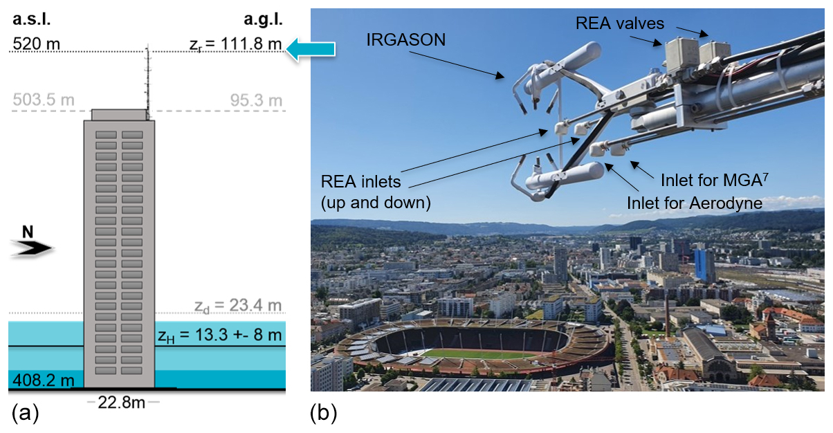
Figure 3 Setup of the Zurich campaign. (a) Schematic illustration of the building Hardau II with the mast, where measurements were made. Also given are the corresponding heights in meters above sea level (m a.s.l.) and above ground level (m a.g.l.). z_H denotes the mean building height within 1.5 km radius, and z_d is the displacement height according to Kanda et al. (2013). (b) Picture of the IRGASON and the inlets for the relaxed eddy accumulation (REA) system, a multi-compound (MGA⁷) gas analyzer, and an Aerodyne for carbonyl sulfide (COS) measurements. The aforementioned instruments were placed in a room on the top floor of the building and connected by 33 m long Synflex tubings.

5 Quality control of REA flask samples

The final setup of the REA flask sampling system, including the chosen materials (Table A1) and the flow scheme with the specially designed loop systems (Fig. 1), was the result of many preliminary assessments, simulations, tests, and iterative system improvements required to meet the high technical requirements of the REA method and the sample analysis. However, due to non-idealities and uncertainties in the sampling procedure, the concentration of the air that is collected in the updraft and downdraft flasks may deviate from the “true” sample concentration that would result from a certain temporal variation in the gas concentration and the vertical wind velocity. To evaluate the performance of the system, i.e., to check for biases and quantify the uncertainty of the flask concentrations due to the sampling process, several experiments and simulations were performed. This section describes the following:

$$\begin{array}{c}{\displaystyle }\begin{array}{ll}\left.\begin{array}{l}\mathrm{5.1}\text{quality control tests in}\\ \text{the laboratory ensuring that}\\ \text{the collected air is generally}\\ \text{transferred into the glass}\\ \text{flasks without contamination}\\ \\ \mathrm{5.2}\text{simulations using}\mathrm{20}\mathrm{Hz}\\ {\mathrm{CO}}_{\mathrm{2}}\text{in situ measurements in}\\ \text{Zurich to estimate biases and}\\ \text{uncertainties in}\mathrm{\Delta }{\mathrm{CO}}_{\mathrm{2}}\text{flask}\\ \text{measurements due to}\\ \text{non-idealities in the sampling }\\ \text{process}\end{array}\right\}& \begin{array}{l}\text{Table 3:}\text{Mean}\\ \mathrm{\Delta }{\mathrm{CO}}_{\mathrm{2}}\\ \text{uncertainties}\end{array}\end{array}\\ {\displaystyle }\begin{array}{l}\mathrm{5.3}\text{quality control tests performed during the Zurich}\\ \mathrm{\text{campaign and comparison of measured flask}}\\ \mathrm{\text{concentrations with in situ measurements to assess}}\\ \mathrm{\text{the quality of the samples collected in Zurich.}}\end{array}\end{array}$$

The focus was on the uncertainty in the CO₂ concentration differences between updraft and downdraft flasks (ΔCO₂) rather than on absolute concentrations because only the concentration differences are needed to calculate fluxes (Eq. 1). Moreover, the flask concentration differences were comparable with high-frequency in situ CO₂ measurements of the IRGASON and a multi-compound (MGA⁷) gas analyzer (MIRO Analytical AG, Wallisellen, Switzerland) despite an irregular calibration of the gas analyzers. It must be noted that, when estimating fossil fuel CO₂ differences, uncertainties due to the sampling process are negligible compared to the ¹⁴C measurement uncertainty (compare Sect. 3 and Appendix D).

5.1 Quality control tests in the laboratory

Several quality control tests were carried out at the ICOS Flask and Calibration Laboratory in Jena to investigate bias or uncertainty due to contamination and memory effects, i.e., the dependence of the measured concentration on the previous sample, for example, due to incomplete evacuation of the buffers. In addition, the rinse time required at the beginning and end of a sampling period was determined by injecting CO₂ pulses.

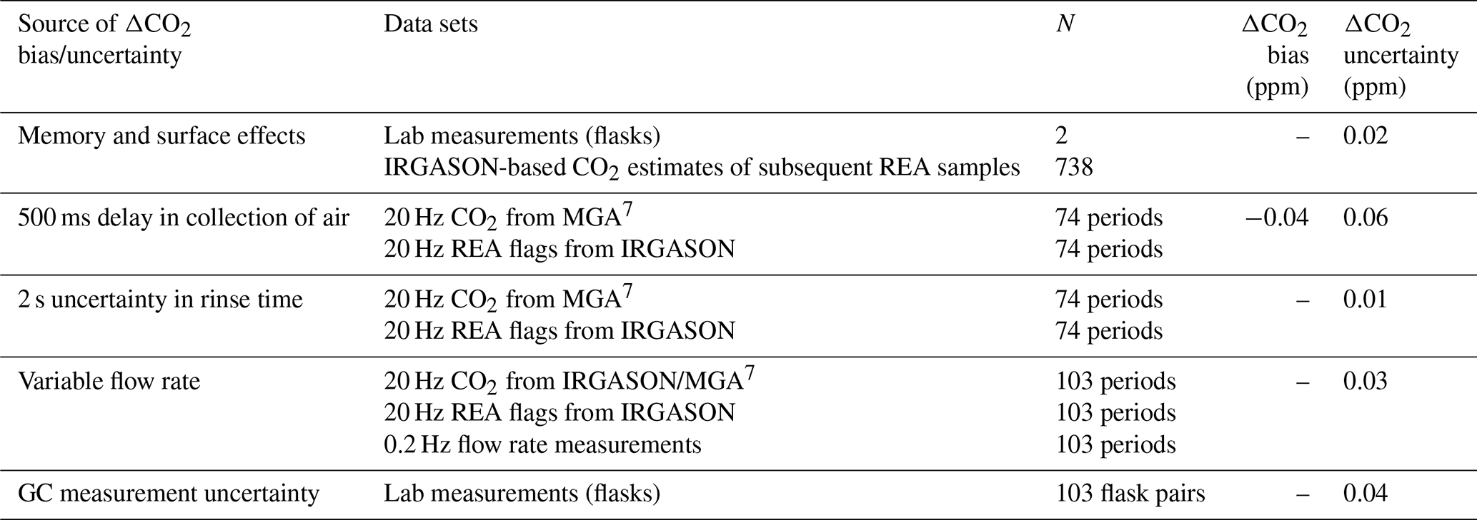
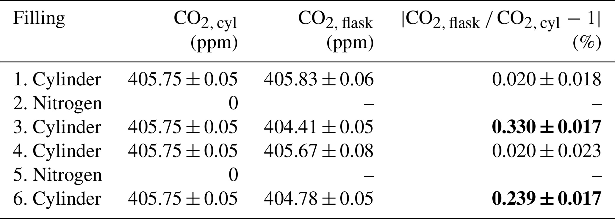
By sampling gas from a cylinder with a known concentration under sampling conditions as close to reality as possible (for details, see Appendix B), it was shown that neither the buffers nor the intake lines or the switching of the valves alter the gas concentrations significantly. As shown in Fig. 4, the CO₂ concentrations of test flasks filled with the sampling system using updraft and downdraft intakes, the loop systems, and buffers agree within 1σ with each other and with the cylinder concentration and mostly meet the WMO compatibility goal for CO₂ of 0.1 ppm (WMO recommendation for the compatibility of measurements of greenhouse gases and related tracers; Tans and Zellweger, 2014).

Figure 4 Deviation of measured flask sample concentrations from the CO₂ concentration of the reference cylinder (405.71 ± 0.01 ppm) that was connected to the fast-response solenoid valves. The gray-shaded area highlights the WMO compatibility goal of 0.1 ppm for CO₂. Details of the experiments are given in Appendix B.

A memory effect was visible after filling one buffer with pure nitrogen (causing a diluted CO₂ concentration of 404.6 ppm measured in the flask compared to 405.8 ppm inserted from the cylinder). During regular operation of the system, however, the differences between two consecutive buffer fillings are much smaller. Based on the measurements during the Zurich campaign, the additional uncertainty of the absolute CO₂ concentration is therefore estimated to be about 0.15 ppm, depending on the CO₂ difference compared to the previous sample (see Appendix B2). The impact on ΔCO₂ is expected to be even smaller (uncertainty of about 0.02 ppm) since the updraft and downdraft samples are usually affected in a similar way.

It was also shown that the time needed to pump an air parcel from the inlet into the buffer as estimated from the flow rates and the volumes of the tubes (Eq. 10) agrees well (within less than 1.5σ) with the measured travel time of an artificial CO₂ pulse (see Appendix B3). This confirms the calculation of the rinse time according to Eq. (10).

5.2 ΔCO₂ uncertainty simulations

The laboratory tests “only” proved the ability to successfully transfer sample air from the REA inlets into the flasks without altering the gas concentration. Several aspects that would affect the measurements in a real REA run, i.e., with a temporally varying gas concentration, were investigated through simulations using the high-frequency CO₂ measurements of the MGA⁷. For this purpose, the 10 Hz time series of the MGA⁷ (available since early August 2022, with a few outages, covering 74 REA sampling periods) was upsampled to 20 Hz and synchronized with the IRGASON data by finding the time lag of maximum correlation between the high-frequency CO₂ measurements. Mean concentrations of the updraft and the downdraft samples could then be simulated from the high-frequency data using the 20 Hz REA flags (Sect. 4.1). In this section, ΔCO₂ uncertainties and potential biases are assessed based on the MGA⁷ data. To make the in situ estimates comparable to the air samples that were dried during the transfer into the flasks (compare Sect. 5.3), the measured gas densities were converted into dry air molar fractions (see Appendix C1).

5.2.1 ΔCO₂ with delayed collection of air

Time lags between a change in the sign of the vertical wind velocity fluctuations w^′ = $w-\stackrel{\mathrm{‾}}{w}$ and the actual collection of air in the respective reservoirs are a known source of uncertainty in REA flux measurements (e.g., Baker et al., 1992; Pattey et al., 1993). In the given setup, the IRGASON measures the vertical wind speed at a frequency of 20 Hz so that the maximum delay between the change in wind speed and its detection is 50 ms. As mentioned in Sect. 4.1, the IRGASON output has, at the maximum bandwidth of 20 Hz, a time delay of 200 ms. With a bandwidth of 10 Hz, as used by default in Zurich, there is a 400 ms delay. The response time of the solenoid valves is 50 ms or less (open) or 150 ms or less (closed). Consequently, it is assumed that the collection of air is delayed by up to 500 ms.

The effect of a delayed collection of air was investigated by calculating the expected CO₂ difference between updraft and downdraft samples of the Zurich REA runs based on the 20 Hz REA flags considering different time lags (see Appendix C3). As expected, the larger the delay, the smaller the concentration differences as air is “sampled” from within the deadband, while portions of the larger signals are missed. On average, a 500 ms delay reduces ΔCO₂ by 0.04 ± 0.06 ppm. If the delay is 100 ms smaller or larger than expected (i.e., 400 or 600 ms), ΔCO₂ changes by less than 0.02 ppm. More results are given in Table C2.

5.2.2 ΔCO₂ with incorrect rinse time

Compared to systems with a single inlet, the direct separation of updraft and downdraft samples close to the ultrasonic anemometer of the IRGASON prevents biases due to uncertainties in the travel time of air from the inlet to the buffer and a potential mixing of air in front of the valves. The travel time, however, becomes important at the start and end of sampling, where the rinse time determines the opening and closing of the magnet valves at the buffers (Sect. 4.2). Given the uncertainties in the pump speeds and the lengths of the tubing, the calculated rinse time (Eq. 10) in the Zurich setup had an uncertainty of about 2 s. This can lead to the sampling of unwanted air and the loss of wanted air. The impact on the concentration difference between the updraft and downdraft flasks was estimated from MGA⁷ data by discarding the first 2 s of measurements in sampling mode and adding another 2 s after the sampling end and vice versa (see Appendix C4). There is no systematic bias, and the standard deviation in the change of ΔCO₂ is 0.01 ppm.

5.2.3 ΔCO₂ with variable sampling rate

Another source of uncertainty is the actual flow rate at which the air is sampled. This flow rate should be constant to ensure a homogeneous weighting of the collected air over time. For this purpose, mass flow controllers were placed right before the buffers. However, the MFCs are slightly affected by humidity and have a response time of 1 to 2 s. This means that, after a change in the pressure difference across the element, it will take up to 2 s for the flow to become constant again. In the REA system, the valves can switch with a frequency of up to 10 Hz, and, with each switching, the pressure behind the MFC changes between atmospheric pressure (standby mode) and the pressure in the buffer (sampling mode). Consequently, the deviation from the desired flow is especially large at the beginning and end of a sampling period, when the pressure in the buffer is 1 mbar or up to 1600 mbar, respectively. In addition, unsynchronized switching of the top valves (20 Hz scan rate) compared to the valves in the loop systems (10 Hz scan rate) can lead to underpressure in the intake line. The greater the underpressure, the higher the flow rate at the inlet when the top valve opens the next time. At the beginning of the Zurich campaign, there were additional biases due to a difference in flow rate during the rinse time compared to during the rest of the sampling period and due to a loss of sample when one of the two buffers reached the maximum pressure of 1.6 bar.

To estimate the effect on the concentration differences between updraft and downdraft flasks, ΔCO₂ was simulated 103 times for each REA run during the Zurich campaign, each time with a different weighting of the MGA⁷ or IRGASON measurements. The weighting was thereby based on actual flow rate measurements of the MFCs (see Appendix C5). While there is no systematic bias, the standard deviation of the ΔCO₂ difference between an inhomogeneous and a homogeneous weighting is, on average, 0.03 ± 0.05 ppm. The deviations are largest during sampling periods with high CO₂ variability, where the absolute ΔCO₂ is also usually larger than average (see Fig. C1). Consequently, the relative uncertainties are less affected. To minimize this uncertainty, the flow rate during the rinse time was adjusted to the flow rate during the sampling period; the maximum buffer pressure, i.e., the pressure at which sampling is stopped, was reduced to 1.55 bar; and an additional pressure regulator was installed in each loop system.

Mean ΔCO₂ uncertainties

Table 3 summarizes the estimated ΔCO₂ biases and uncertainties due to the different aspects mentioned above. It is important to note that the given means and standard deviations are solely based on data from the 103 REA runs during the Zurich campaign and a small number of quality control tests. The results may be different for other time periods and other sites. However, the estimates show that, except for a delayed collection of air, there is no bias in the concentration differences between updraft and downdraft samples. The standard deviations of the data set, on the other side, are of the order of the ΔCO₂ measurement uncertainty at the gas chromatograph (GC). This means that, for individual samples, e.g., those collected during periods of high variability in the CO₂ concentration of the ambient air, the flow variability and other non-idealities in the sampling process can be significant sources of ΔCO₂ uncertainty. Regular quality control tests and comparisons of flask samples with in situ measurement data are therefore important for independent validation of the performance of the system during a measurement campaign (see Sect. 5.3). Due to dependence on the ambient sampling conditions, the different ΔCO₂ uncertainty contributions should, in this case, be considered for each sampling period individually.

Table 3 Overview of the estimated biases and uncertainties in the CO₂ concentration differences between updraft and downdraft flasks (ΔCO₂) due to non-idealities in the sampling procedure. Given are the means (bias) and standard deviations (uncertainty) of the measured or simulated changes in ΔCO₂ with respect to the expected values. For completeness, the measurement uncertainty of the gas chromatographic analysis of the flasks is also given. N represents the number of measurements or sampling periods for the underlying data set.

On the contrary, to estimate ffCO₂ differences, the measurement uncertainty of ¹⁴CO₂ is by far the dominant source of uncertainty (see Appendix D). Moreover, when estimating ffCO₂ fluxes, β calculated from CO₂ for each REA run individually accounts for most of the above-mentioned effects (Pattey et al., 1993). In this case, the uncertainties due to the sampling process are considered to be negligible.

5.3 Quality control tests during the campaign

To ensure that the REA flask sampling system was working as intended, quality control tests were performed regularly throughout the Zurich campaign. In addition, the measured concentration differences of the REA flask pairs were compared with the in situ measurements of the IRGASON and the MGA⁷.

5.3.1 All-valves-open tests

To check for biases between updraft and downdraft sampling, as well as for leaks or other sources of contamination, “all-valves-open” tests were performed about once a month. This involved continuously filling two buffers with ambient air by turning on the pumps and opening both solenoid valves at the inlets, as well as the valves in the loop systems, until a buffer pressure of about 1.4 bar was reached and the samples could be transferred into the flask sampler. Biases between updraft and downdraft lines would result in concentration differences between the two corresponding flasks. To detect systematic errors that might affect both lines equally, a third flask was sampled simultaneously through a separate tube directly into the flask sampler, bypassing the REA loops and the buffers. In this case, the flow rate through the flask was reduced over sampling time t according to $\mathrm{1}/t$ as flask concentrations then best reflect the real mean concentrations (Levin et al., 2020). If the system is working as expected, the concentrations in the three flasks should agree within the WMO compatibility goal. Another quality control would be to compare the absolute concentrations of the flasks with the average concentration of in situ measurements over the sampling period. In Zurich, however, no accurate measurements of ambient air near the inlets were available (neither the IRGASON nor the MGA⁷ were meant to be calibrated regularly according to WMO standards).

During the Zurich campaign, nine all-valves-open tests were performed. Figure 5 shows the CO₂ concentration of each flask compared to the respective mean of the “up” and “down” samples. In tests 2, 3, 7, 8, and 9, an additional flask was sampled directly into the flask sampler. However, it was later found that, at least at the beginning of the sampling periods, the flow rate was lower than intended. This means that the air in the direct flasks could not be exchanged sufficiently, such that the concentration does not represent the actual mean value but is also influenced by the purging period preceding the sampling. This particularly affects the flasks that were collected during a period with a large variability in concentration.

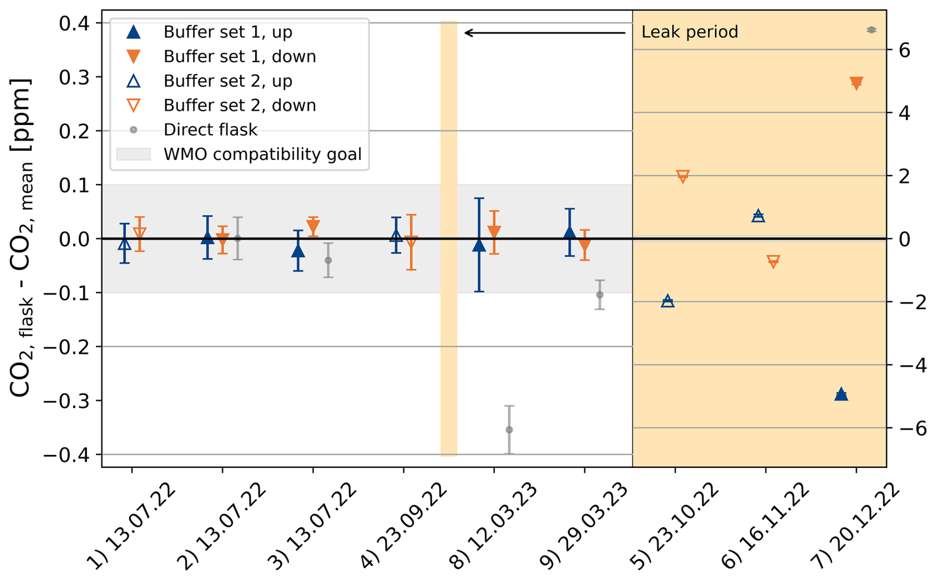
Figure 5 Comparison of flask concentrations from all-valves-open tests. Shown are the differences in CO₂ between flasks sampled through the updraft and downdraft intakes of the REA system and a flask sampled directly into the flask sampler compared to the mean of the two samples from the REA intake system. Large deviations in tests 5, 6, and 7 (beige-shaded parts with different scales on the y axis) were caused by two leakages in the loop systems. Outside this period, the results mostly agree within the WMO compatibility goals.

It can be seen that, for tests 1, 2, 3, 4, 8, and 9, up and down flasks agree within their measurement uncertainties, indicating that there is no significant bias between the two lines. The difference between the pairs of simultaneously collected flasks is, on average, −0.01 ± 0.03 ppm. The smaller CO₂ concentrations of the direct flasks of tests 8 and 9 can be explained by a large CO₂ variability with an overall increase over time. The fact that, in tests 2 and 3, up and down flasks also agree with the direct sample within the WMO compatibility goal indicates that there was no bias from the loop system or from the buffers that would have affected the up and down flasks in the same way.

In tests 5, 6, and 7, on the contrary, there are large concentration differences between up, down, and direct flasks (note the different scales on the y axis). This indicates a leak in the system, which also explains the large deviations of the measured CO₂ concentrations from the expected CO₂ concentrations based on in situ measurements observed at this time (compare with the next section). Unfortunately, due to the long time lag between sampling and the availability of concentration measurements, the leak could only be detected and fixed after several months.

In summary, the results show that, in general, there is no significant bias between updraft and downdraft sampling and that all-valves-open tests help detect leaks.

5.3.2 Flask – in situ comparison

In addition to the all-valves-open tests, the measured concentration differences of the REA flask pairs were compared to in situ measurements from the IRGASON and the co-located MGA⁷ by averaging the high-frequency data from the periods during which the respective valves were open and air was sampled, as denoted by the 20 Hz REA flags (see Appendix C2). For the final ΔCO₂ estimates, uncertainties of $\sqrt{\mathrm{2}}$ ⋅ 0.15 ppm for the IRGASON estimates and $\sqrt{\mathrm{2}}$ ⋅ 0.1 ppm for the MGA⁷ estimates were assumed based on the precision of the instruments as stated by the manufacturers. For the flask data uncertainty, the GC measurement uncertainties and the individually simulated sampling uncertainties from a memory effect, an uncertainty in the time lag between the vertical wind signal and the conditional collection of air, an uncertainty in the rinse time, and an inhomogeneous weighting of sample air due to variability in the sampling rate were taken into account (compare to Table 3).

The results of 102 REA runs during the Zurich campaign are shown in Fig. 6, which plots the differences between ΔCO₂ from flask measurements and in situ estimates from the IRGASON and the MGA⁷ over the sampling time (for 1 of the 103 REA selected runs, neither IRGASON nor MGA⁷ data are available). The samples from November 2022 to February 2023, which were contaminated due to a leak (Sect. 5.3), were discarded.

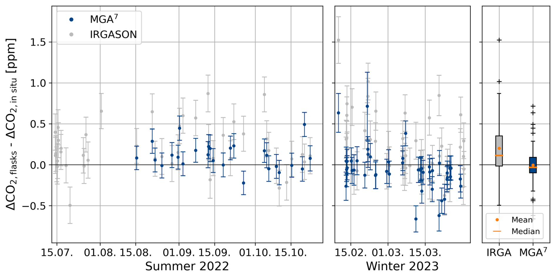
Figure 6 Difference between ΔCO₂ (up−down) measured in the flasks and estimated from high-frequency measurements of the IRGASON and the MGA⁷. Error bars represent the flask measurement uncertainty (analysis plus estimated uncertainty due to the sampling process) and an estimated uncertainty of 0.15 ppm for the IRGASON and 0.1 ppm for the MGA⁷. MGA⁷ data are only available from the middle of August. The leak period between the end of October and the beginning of February and the measurements by the IRGASON of CO₂ signal strength < 90 % and the correlation with the MGA⁷ < 0.5 were excluded. The boxplot on the right shows the mean, median, and interquartile range of all summer and winter samples.

The fact that the MGA⁷ estimates agree very well with the flask measurements (mean difference in ΔCO₂ < 0.01 ppm, with a standard deviation of 0.23 ppm) provides evidence that there were no major leaks or significant biases due to the sampling process. A potential bias due to a delayed collection of air (Sect. 5.2.1) is therefore considered to be negligible. Four ΔCO₂ measurements deviated from the expected value by more than 0.5 ppm. The exact reasons are not known, but, for example, during the REA run on 21 February 2023 (07:00–08:00 LT), the CO₂ concentration increased by more than 100 ppm, and the CO₂ difference between the updraft and downdraft samples was the highest observed. During the REA run on 11 March 2023 (13:30–14:30 LT), the wind measurements were very spiky, likely due to a rain event earlier in the day, and, according to the REA flags, the valves did not switch as one would expect from the wind data. These sampling periods must therefore be examined more closely before further analysis.

The IRGASON-based ΔCO₂ estimates deviate significantly more from the flask measurements, with an average of 0.20 ± 0.33 ppm. This, however, could be linked to the fact that the IRGASON CO₂ dry molar fractions were derived from a CO₂ density output that does not properly account for high-frequency fluctuations in air temperature in the sensing path because the ambient temperature measured by the EC100 slow-response temperature probe is used in the conversion of absorption measurements into CO₂ density (see Appendix C1). As described by Helbig et al. (2016), this causes a systematic bias compared to closed-path gas analyzers due to the high-frequency temperature attenuation. Indeed, the difference between ΔCO_2, flasks and ΔCO_2, IRGA correlates with the difference between ultrasonic temperature during updraft and downdraft conditions. Helbig et al. (2016) showed that this bias could be reduced significantly by using the ultrasonic anemometer's fast-response temperature. Due to a lack of knowledge, this additional CO₂ density output, where the high-frequency temperature is used in the absorption-to-density conversion, was not recorded during the Zurich campaign. Since the differences between IRGASON and flask measurements could be explained by the insufficient correction of spectroscopic effects during high sensible heat fluxes, the good agreement between flask data and MGA⁷ measurements indicates an overall successful implementation of the REA method.

6 ΔCO₂ partitioning

Figure 7 shows the differences in CO₂ and ffCO₂ between the updraft and downdraft flasks, measured with the gas chromatograph at the ICOS FCL in Jena and derived from the ¹⁴CO₂ analyses at the ICOS CRL in Heidelberg (Eq. 9). Of the 103 REA flask pairs selected for laboratory analysis and analyzed for CO₂ at the FCL (Sect. 4.5), 3 samples were lost during graphitization at the CRL. Eight sample pairs from the end of the campaign were not analyzed for ¹⁴CO₂ because their total CO₂ difference was small, and the expected significance of the ¹⁴CO₂ analysis was low compared to the associated costs. This leaves a total of 92 ΔffCO₂ estimates. The error bars represent the measurement uncertainties (ΔCO₂ uncertainties of about 0.05 ppm in x direction are omitted for clarity). In the analysis of ffCO₂, uncertainties due to the sampling process were considered to be negligible (Sect. 5). The colors indicate the month in which the sample was collected.

Figure 7 ΔffCO₂ and ΔCO₂ of the 92 selected REA flask pairs from Zurich.

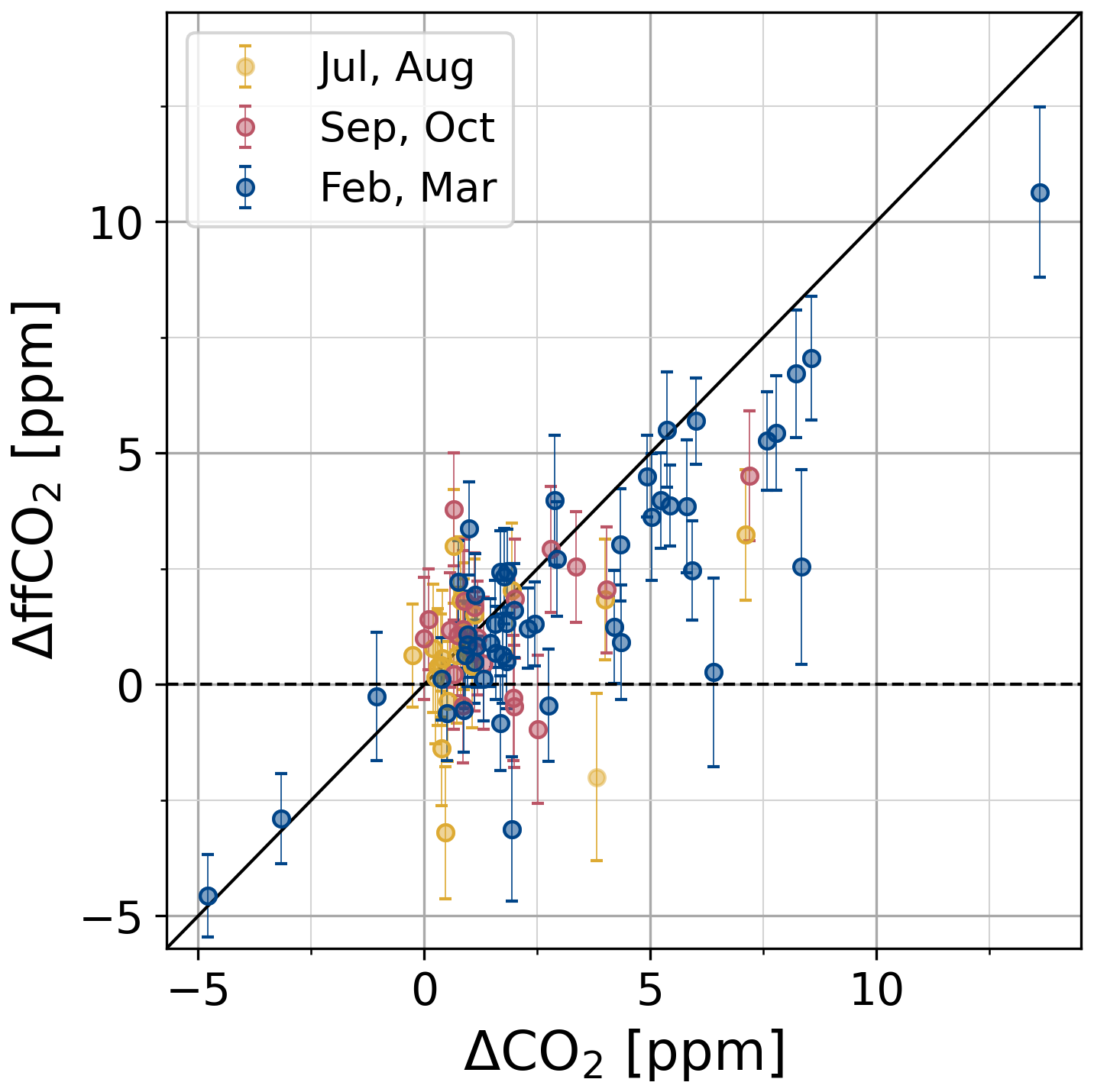
It can be seen that the largest concentration differences between updraft and downdraft flasks with ΔCO₂ of up to 13.6 ppm were collected in February and March, when anthropogenic emissions are usually higher than average due to residential heating. Most of these samples are close to the 1:1 line, which represents the case where the net non-fossil CO₂ flux is zero and the measured CO₂ fluxes are completely due to fossil fuel emissions. Accordingly, the observed deviations from this line to the right or the left indicate dominant respiratory and other non-fossil sources or photosynthetic signals, respectively. For samples along the x axis, the ffCO₂ contribution is approximately zero. In agreement with other studies (e.g., Wu et al., 2022; Miller et al., 2020; Crawford and Christen, 2015; Turnbull et al., 2015), this shows that there are significant non-fossil CO₂ signals even in winter.

It should be noted that the applied sample selection criteria do not necessarily exclude sampling periods in which a change in the storage below the sampling height contributes to the measured fluxes. This is the case, for example, when the depth of the atmospheric boundary layer increases rapidly due to convective, turbulent vertical motions generated by radiative heating of the surface in the morning (Stull, 1988). Based on an observed drop in CO₂ concentration in the morning and a preliminary investigation of the turbulence structure of the atmosphere, some of the Zurich REA flasks with large CO₂ concentration differences between updraft and downdraft samples were probably collected during this time. In this case, the composition of the samples does not necessarily represent the actual surface fluxes during the REA sampling periods but rather represents the integrated nocturnal fluxes. Further interpretation of the results and a subsequent investigation of the corresponding CO₂ fluxes therefore require a thorough analysis of the sampling periods.

What also becomes clear in Fig. 7 is that most signals are of the order of 1 ppm or less, which is small compared to the ΔffCO₂ uncertainty. The latter was, on average, 1.2 ppm and was primarily due to the mean ¹⁴CO₂ measurement precision of 1.8 ‰ (Appendix D). Consequently, ffCO₂ flux estimates derived from samples with ΔffCO₂ < 1.2 ppm will mostly have uncertainties of more than 100 % (compare to Eq. 2). This highlights the importance of further quality control of the existing data set for subsequent calculations and quantitative analyses of ffCO₂ fluxes.

7 Conclusions

A relaxed eddy accumulation (REA) flask sampling system for ¹⁴C-based estimation of ffCO₂ fluxes for urban eddy covariance (EC) flux measurements was developed and tested in the ICOS Flask and Calibration Laboratory in Jena, Germany, and on a tall tower near the city center of Zurich, Switzerland.

Two fast-response valves are activated by the vertical wind signal from an ultrasonic anemometer of a co-located IRGASON. The conditionally collected air accumulates in two separate cylinders (one for the updraft sample and one for the downdraft sample) and is transferred into 3 L glass flasks after the sampling period using an automated 24-port flask sampler. The samples can thus be analyzed in the laboratory for a variety of gases, including ¹⁴CO₂. Laboratory tests and quality control tests during the first measurement campaign in Zurich showed that the sampling procedure does not cause a significant bias in the CO₂ differences between updraft and downdraft samples. Uncertainties due to the sampling process are negligible when estimating fossil fuel CO₂ differences between the updraft and downdraft flasks and, consequently, ffCO₂ fluxes as these are dominated by the ¹⁴CO₂ measurement precision. The novel REA flask sampling system itself fulfills the high technical requirements of relaxed eddy accumulation, providing high-quality data for scientific studies of multiple non-reactive species.

Due to the prerequisites of the EC and REA method, e.g., stationarity and well-developed turbulence, and the costs and efforts associated with the flask analysis, only a limited number of individual sampling periods can be analyzed. In general, operating the system, i.e., scheduling sampling events, analyzing and selecting suitable sampling periods, sending the flasks to the laboratory, etc., requires frequent remote and on-site work.

Given the good agreement between the total CO₂ concentration differences measured in the REA flask sample pairs and observed from in situ measurements of an MGA⁷, the results of the first measurement campaign in Zurich serve as a proof of concept for a ¹⁴C-based separation of fossil and non-fossil CO₂ signals. As expected, the CO₂ differences between updraft and downdraft samples were largest during the heating season in February and March. In this case, fossil fuel emissions were the major contributor. However, even in winter, small photosynthetic and significant non-fossil (respiration and biofuels) signals were observed, highlighting the role of the biosphere in an urban environment.

The main challenge so far was a generally small signal-to-noise ratio of measured ¹⁴CO₂ differences. Resulting ΔffCO₂ uncertainties on the order of 100 % limit the interpretation of individual results. However, a new accelerator mass spectrometer has reduced the Δ¹⁴ measurement uncertainty and, thus, the ΔffCO₂ uncertainty by about 23 %, which will increase the fraction of usable samples in future applications.

Two improvements are proposed to further increase the concentration differences in future campaigns: first, the two pumps in the loop systems are recommended to be replaced by larger pumps with a higher pump speed, allowing a reduction in the proportion of time that air is collected and, thus, a larger deadband width δ. Second, the so-called hyperbolic relaxed eddy accumulation could be added into the logger program. With this setting, as proposed by Bowling et al. (1999), air would only be collected if the fluctuations in vertical wind speed w^′ and concentration c^′ are above a certain threshold. For the latter, the 20 Hz CO₂ measurements of the IRGASON could be used. Excluding eddies with little flux contribution increases the concentration differences more effectively than a linear deadband with larger deadband width and is recommended for scalars where the detection limit is of concern (Vogl et al., 2021). However, the hyperbolic deadband comes with additional challenges as the threshold for not only vertical wind velocity fluctuations but also CO₂ mixing ratio fluctuations would need to be dynamically adjusted. The signal-to-noise ratio could also be increased if multiple graphite targets were to be analyzed or if measurements were to be taken closer to a particular source. However, obtaining and analyzing multiple flask samples would require major changes in the setup of the flask sampler and would multiply the cost and instrument time accordingly. In addition, analyzing turbulent fluxes on a neighborhood scale requires tall-tower measurements within the inertial sublayer. Besides limitations in the availability of the corresponding infrastructure, reducing the measurement height was therefore not an option for our study.

The next step in the process will be to derive the actual ffCO₂ fluxes using EC-based total CO₂ fluxes and assuming scalar similarity to estimate the β coefficient for each sampling period individually (Eq. 2). This will allow for a fully independent time-resolved evaluation of the Zurich emission inventories, taking into account the changing turbulent flux footprints during each of the sampling intervals. Furthermore, the analysis of CO and other species in the updraft and downdraft samples along with ¹⁴CO₂ will provide guidance regarding the use of co-emitted species for partitioning total CO₂ fluxes into fossil and non-fossil components.

Appendix A: Setup of the REA flask sampling system

Figure A1 Photo of the REA flask sampling system as installed in the control room below the tower at Zurich–Hardau. (1) Screen with flask sampler software. (2) Connection to the CR6 data logger. (3) Intake lines. (4) Loop system. (5) Buffers. (6) Air dryer. (7) Flasks.

Table A1 Components of the REA flask sampling system (compare Figs. 1 and 2).

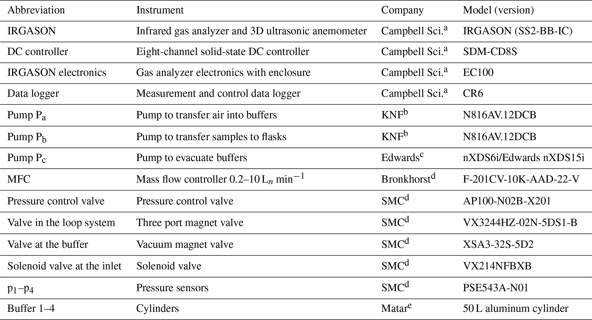
^a Campbell Scientific Inc., Logan, UT, USA. ^b KNF Neuberger GmbH, Freiburg, Germany. ^c Edwards Vacuum, Burgess Hill, UK. ^d SMC Corporation, Tokyo, Japan. ^e Matar, Mazzano, Italy.

Appendix B: Laboratory tests

B1 Contamination test 1

To test for a potential contamination of the samples during the sampling process, e.g., due to a leak in the line or at the valves or due to surface effects with the surfaces of tubes and buffers, the REA system was set up in the laboratory of the ICOS FCL in Jena. For practical reasons, the IRGASON and the fast-response valves were placed in the same room as the buffers and the flask sampler but were connected through two > 50 m long Synflex tubes. A reference gas cylinder with 407.71 ± 0.01 ppm CO₂ was connected to a custom dew point generator. In this way, the humidity of the gas was comparable to that of typical ambient air (dew point of approximately 12 °C), thus avoiding increased or reduced surface effects along the tube and in the buffers, which could result from a change in water availability (Zhao et al., 2020). The humidified gas was then directed through a three-way valve to the solenoid valves and sampled into the respective buffers according to a wind signal from the IRGASON, artificially generated through a fan. From there, the gas was transferred into the flask sampler as during a regular REA run. The test was repeated five times, with slightly different setups as listed in Table B1. The results are given in Fig. 4.

B2 Contamination test 2: memory effect test

Although the first set of contamination tests (Sect. B1) had already shown that the concentration of the sample is not significantly changed by the sampling process, a second experiment was performed to quantify the influence of the previous sampling on the flask concentration. For this purpose, a cylinder with a known gas concentration and pure nitrogen were alternately connected to the loop systems via an approximately 80 m long Synflex tube with an 8 mm outer diameter. As in first contamination tests (Sect. B1), the dry gas from the tanks was humidified through a custom dew point generator to a dew point of approximately 12 °C, comparable to normal sampling conditions of ambient (humid) air. All valves were opened, and one buffer (always buffer 4) was filled six times to approximately 1.2 bar. The cylinder gas was then transferred into the flask sampler, and the buffer was evacuated again (residual buffer pressure of about 0.6 mbar). The CO₂ concentrations measured in the respective flasks are given in Table B2.

Table B1 List of differences between the six setups for contamination tests in the laboratory.

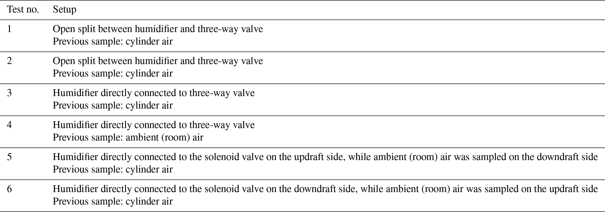
Table B2 CO₂ concentrations of the flasks compared to the reference gas cylinder that was connected to the inlets before and after sampling pure nitrogen. The results are given in chronological order of the fillings.

While the CO₂ concentrations of flasks 1 and 4 agreed with the cylinder gas within 1.5σ, flasks 3 and 6, collected after flushing the system with nitrogen, i.e., after an intentionally chosen large CO₂ change of 405.7 ppm, deviated by more than 1 ppm. Assuming that the bias in the flask concentration c_meas − c_ref (measured minus reference concentration) depends linearly on the concentration difference between the current and the previous sample c_ref − $c_{\mathrm{ref},-\mathrm{1}}$, it can therefore be expected that CO${}_{{\mathrm{2}}_{\mathrm{meas}}}$ − CO${}_{{\mathrm{2}}_{\mathrm{ref}}}$ = $(\mathrm{0.0028}\pm \mathrm{0.0005})\cdot ({{\mathrm{CO}}_{\mathrm{2}}}_{\mathrm{ref}}-{{\mathrm{CO}}_{\mathrm{2}}}_{\mathrm{ref},-\mathrm{1}})$. As an uncertainty, half of the difference between the two measurements was taken. Based on the IRGASON-derived CO₂ estimates of the updraft and downdraft samples of all REA sampling periods during the Zurich campaign (702 in total), the mean concentration difference between subsequent buffer fillings was estimated to be 0 ± 52 ppm (assuming that buffer sets 1 and 2 are always used alternately). Consequently, there is no systematic bias in absolute flask concentrations, while the estimated uncertainty is 0.17 ppm.

Since the updraft and downdraft samples are usually affected in a similar way, the effect on concentration differences between them is expected to be even smaller. Multiplying the mean difference between subsequent concentration differences between updraft and downdraft sampling (estimated again from the IRGASON data) of 0 ± 7 ppm with the 0.28 ± 0.05 % derived from the laboratory experiments (Table B2) results in an estimated uncertainty of about 0.02 ppm. Again, there is no systematic bias.

B3 Rinse time measurements

In the field, the rinse time, i.e., the time between the start (end) of the sampling period and the opening (closing) of the valves at the buffers, is calculated from the estimated pump speed and the dimensions of the intake lines according to Eq. (10). To test the validity of this approach and to quantify the associated uncertainty, a cylinder with pure CO₂ was connected at the normally closed position of a three-way valve installed in front of the fast-response valves. The loop system was in sampling mode (pump on, three-way valves in the loop systems connecting the pump with the outflow). Then, the three-way valve was opened to the CO₂ cylinder for 200 ms, injecting a short CO₂ pulse into the line. This pulse was detected at the outflow of the REA sampler by a CO₂ sensor (SprintIR-WF-20, Gas Sensing Solutions Ltd, Cumbernauld, UK). The travel time of the CO₂ pulse was thus estimated as the time between the opening of the three-way valve and the start of the detected spike. The experiment was repeated several times and for different tubes (see Table B3). The measurements $t_{\mathrm{r},\mathrm{meas}.}$ were then compared to the values $t_{\mathrm{r},\mathrm{est}.}$ estimated from the length and inner radius of the tube and the flow rate measured at the outflow of the REA sampler. As shown in Table B3, both values agreed within less than 1σ.

Table B3 Length l_t and inner diameter r_t of the tubes connecting the REA inlets with the loop systems. Together with the pump flow velocity q_pump (flow rate measured at the outflow), the travel time from the inlet to the outflow $t_{\mathrm{r},\mathrm{est}.}$ was estimated according to Eq. (10) and compared with $t_{\mathrm{r},\mathrm{meas}.}$, which was measured with a CO₂ pulse.

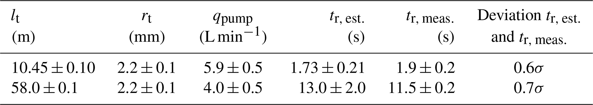
The experiment was also done when the REA valves opened or closed once per second and were therefore only open half the time. As expected, the time until the signal was detected was approximately twice as long as when the valves were permanently open. This suggests that the concept of the rinse time also works well at the start of an REA run when the valves are already switching according to the wind signal.

Appendix C: ΔCO₂ simulations

For uncertainty estimation and quality control, the expected CO₂ differences between the updraft and downdraft samples collected in Zurich were calculated from the high-frequency in situ measurements of the IRGASON and the MGA⁷. This required the synchronization between IRGASON and MGA⁷ data and the start and end times of the REA runs, despiking of the 20 Hz time series according to Mauder et al. (2013), and conversion of measured gas densities into dry molar fractions. The high-frequency measurements were then averaged over the time periods when the updraft and/or downdraft valve was open and air was collected using the 20 Hz REA flags (Sect. 4.1).

C1 Conversion to dry molar fractions

Flask “concentrations” measured at the gas chromatograph are given in moles of gas per mole of dry air, i.e., molar mixing ratio. To compare them with in situ measurements, the 20 Hz humid air mole fractions χ_gas recorded by the MGA⁷ and the mole densities d_gas from the IRGASON were converted into dry air molar mixing ratios as shown below (compare to Mauder et al., 2021; EddyPro Software version 7.0 , 2023).

• MGA⁷:

  $$\begin{array}{}\text{(C1)}& r_{\mathrm{gas}}={\displaystyle \frac{{\mathit{\chi }}_{\mathrm{gas}}}{\mathrm{1}-{\mathit{\chi }}_{{\mathrm{H}}_{\mathrm{2}}\mathrm{O}}}}.\end{array}$$

• IRGASON:

  $$\begin{array}{}\text{(C2)}& r_{\mathrm{gas}}=d_{\mathrm{gas}}{\displaystyle \frac{v_{\mathrm{a}}}{\mathrm{1}-{\mathit{\chi }}_{{\mathrm{H}}_{\mathrm{2}}\mathrm{O}}}}.\end{array}$$

  v_a = $\frac{R\cdot T_{\mathrm{a}}}{p}$ is the ambient air molar volume. Following Helbig et al. (2016), the ambient air temperature T_a is derived from the fast-response ultrasonic temperature corrected for humidity effects (Schotanus et al., 1983):

  $$\begin{array}{}\text{(C3)}& {\displaystyle }{T}_{\mathrm{a}}={\displaystyle \frac{T_{\mathrm{s}}}{\mathrm{1}+\mathrm{0.51}\cdot q}},\text{(C4)}& {\displaystyle }q={\displaystyle \frac{{\mathit{\rho }}_{{\mathrm{H}}_{\mathrm{2}}\mathrm{O}}}{{\mathit{\rho }}_{\mathrm{a}}}}={\displaystyle \frac{{\mathit{\rho }}_{{\mathrm{H}}_{\mathrm{2}}\mathrm{O}}}{{\mathit{\rho }}_{{\mathrm{H}}_{\mathrm{2}}\mathrm{O}}+{\mathit{\rho }}_{\mathrm{d}}}},\text{(C5)}& {\displaystyle }{\mathit{\rho }}_{\mathrm{d}}={\displaystyle \frac{p_{\mathrm{a}}-e}{T\cdot R_{\mathrm{d}}}},\text{(C6)}& {\displaystyle }e={\mathit{\rho }}_{{\mathrm{H}}_{\mathrm{2}}\mathrm{O}}\cdot R_{\mathrm{v}}\cdot T.\end{array}$$

  For calculating the specific humidity q, the slow-response air temperature T measured by a co-located EC100 thermistor at a resolution of 1 s is used.

The various variables are described in Table C1. Note that, for flux calculations in EddyPro, the raw, high-frequency measurements were not converted from molar densities into mixing ratios, but the Webb–Pearman–Leuning (WPL) density corrections Webb et al. (1980) were applied.

C2 ΔCO₂ estimates from IRGASON and MGA⁷ measurements

To calculate the expected CO₂ concentration differences between the updraft and downdraft sample pairs collected in Zurich, the synchronized, despiked, and dry-molar-fraction-converted 20 Hz CO₂ measurements were averaged over the periods where, according to the 20 Hz REA flags, air should have been collected in the updraft and/or downdraft reservoir. For the IRGASON data, four sampling periods with low correlation between the CO₂ of the IRGASON and the MGA⁷ (Pearson correlation coefficient of < 0.5) due to the low CO₂ signal strength of the IRGASON (< 90 %) were discarded.

Table C1 Description of variables used in the conversion of mole fractions and mole densities to molar mixing ratios.

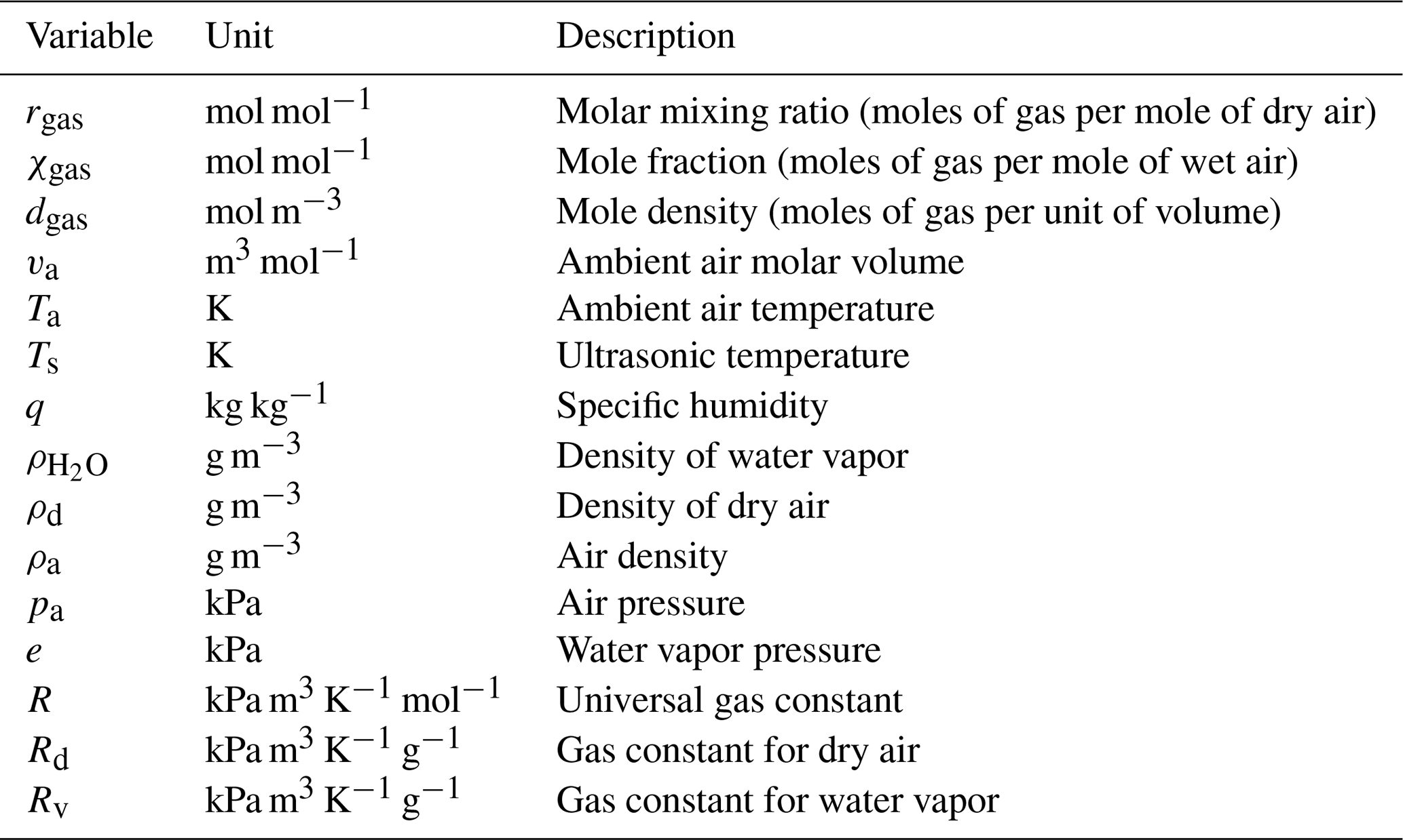
Table C2 Differences between ΔCO₂ simulated with and without time lags between w and CO₂ based on 20 Hz CO₂ measurements of the MGA⁷. Given are the mean and standard deviation (SD), as well as the 0.25th, 0.5th, 0.75th, and 1st quantiles of the Zurich REA runs (n = 74).

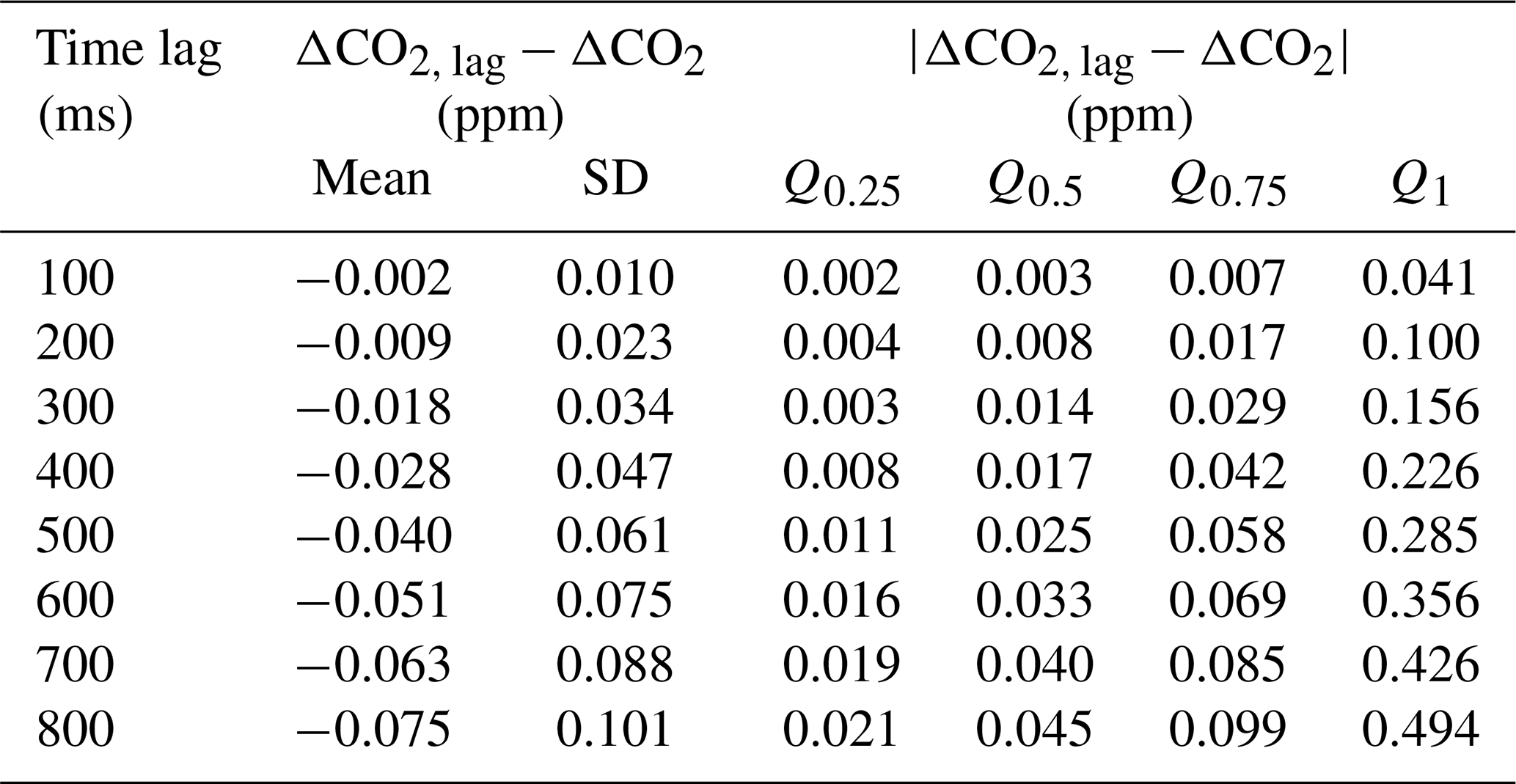
C3 ΔCO₂ with delayed collection of air

To estimate the potential bias and uncertainty caused by a certain time lag between the wanted and the actual collection of air, the CO₂ differences between REA sample pairs were calculated by shifting the 20 Hz REA flags forward in time and then averaging over the periods where the updraft or downdraft valves were open. These values were then compared to the ΔCO₂ estimates calculated without time lag (Sect. C2). Table C2 shows the statistics of the differences in ΔCO₂ with and without the time lag for the 74 REA sampling periods in Zurich where MGA⁷ data are available. The increasingly negative mean ΔCO₂ differences show that ΔCO₂ is systematically reduced when the collection of air is delayed. This is to be expected since, in this case, air is collected when the vertical wind is within the deadband and CO₂ fluctuations are usually smaller than outside the deadband. With a time lag of 500 ms, as is expected in the Zurich setup, ΔCO₂ is, on average, 0.04 ± 0.06 ppm smaller than in the ideal case without a delay; 0.06 ppm is therefore considered to be the mean uncertainty due to a 500 ms delay in the collection of air. For 75 % of the REA runs, the change in ΔCO₂ is less than 0.06 ppm, whereas the maximum simulated difference is 0.29 ppm. However, there is no systematic bias observed in the comparison between flasks and in situ (Fig. 6).

C4 ΔCO₂ with incorrect rinse time

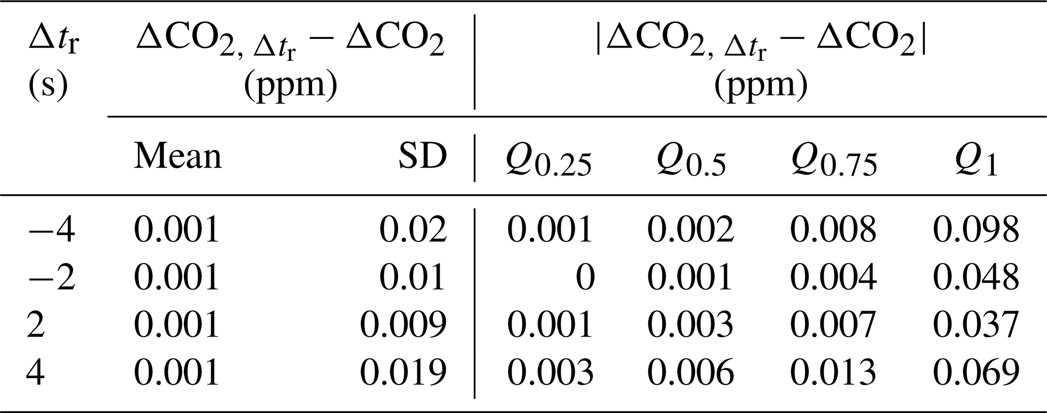
Uncertainty in the time an air parcel needs to travel from the inlet to the buffers (about 2 s in Zurich) can cause sampling of unwanted air and loss of wanted air at the beginning and end of an REA run. If the rinse time were to be longer than the actual travel time by Δt_r (s), the first Δt_r seconds of sampled air would be lost, while air from Δt_r seconds after the intended REA run end would be sampled. Similarly, if the rinse time were to be shorter than the actual travel time by Δt_r, unwanted air remaining in the intake lines would be sampled into the buffers, while the sample air from the last Δt_r seconds in sampling mode would be lost. This was simulated by discarding and adding 20 Hz CO₂ measurements from the corresponding time periods and comparing the estimated concentration differences between updraft and downdraft samples (ΔCO${}_{\mathrm{2},\mathrm{\Delta }{t}_{\mathrm{r}}}$) with the (ideal) estimates where Δt_r = 0 s. The statistics from the 74 REA sampling periods in Zurich with MGA⁷ data are shown in Table C3. The mean difference between ΔCO₂ with and without error in the rinse time is 0.001 ppm and so is well below the CO₂ measurement uncertainty of the flask samples. For individual REA runs, however, a 2 s overestimation or underestimation of the rinse time can change ΔCO₂ by up to 0.5 ppm. The standard deviation of about 0.01 ppm with Δt_r = ± 2 s is considered to be the ΔCO₂ uncertainty of the Zurich samples due to the 2 s uncertainty in the rinse time. The fact that this standard deviation and the median and maximum differences are about twice as large when Δt_r = ± 4 s shows that this uncertainty contribution is site specific.

Table C3 ΔCO₂ simulated from MGA⁷ in situ measurements assuming different errors Δt_r in the rinse time. Positive or negative Δt_r indicate whether the rinse time was overestimated or underestimated. Given are the mean and standard deviation (SD), as well as the 0.25th, 0.5th, 0.75th, and 1st quantiles of the differences in relation to the ideal case without Δt_r = 0 for the Zurich REA runs (n = 74).

C5 ΔCO₂ with variable sampling rate

Under real sampling conditions, a certain variability of the flow rate and, thus, an inhomogeneous weighting of the concentration over time are to be expected, adding uncertainty into the ΔCO₂ flask measurements. To estimate this uncertainty for each REA flask pair, the CO₂ concentration differences between updraft and downdraft samples were simulated from the high-frequency CO₂ measurements of the MGA⁷ or, if not available, the IRGASON (compare to Appendix C2) but this time with different weightings for each 20 Hz measurement. A total of 103 weighting functions were therefore calculated by interpolating the 103 flow rate time series (temporal resolution of 5 s) recorded by the two mass flow controllers in the loop systems during the Zurich REA runs in relation to the 20 Hz CO₂ in situ measurements of each REA run. This resulted in 103 ΔCO₂ estimates for each REA run. The standard deviations of these estimates were then considered to be the ΔCO₂ uncertainty due to flow rate variability. The mean uncertainty of the 103 REA runs was 0.03 ± 0.05 ppm. As shown in Fig. C1, the magnitude depends on the CO₂ variability of the ambient air. In the extreme case of a standard deviation of the ambient CO₂ of more than 50 ppm, the estimated uncertainty can be as high as 0.38 ppm. On the other hand, if CO₂ is approximately constant, the weighting does not matter. In the analysis of ΔCO₂, e.g., in the comparison of flasks with in situ measurements (Sect. 5.3), it is therefore recommended to consider the uncertainty contributions for each REA sample individually. For the estimation of ΔffCO₂, on the other hand, the uncertainty due to flow rate variability is still negligible compared to the ¹⁴C measurement uncertainty (Appendix D).

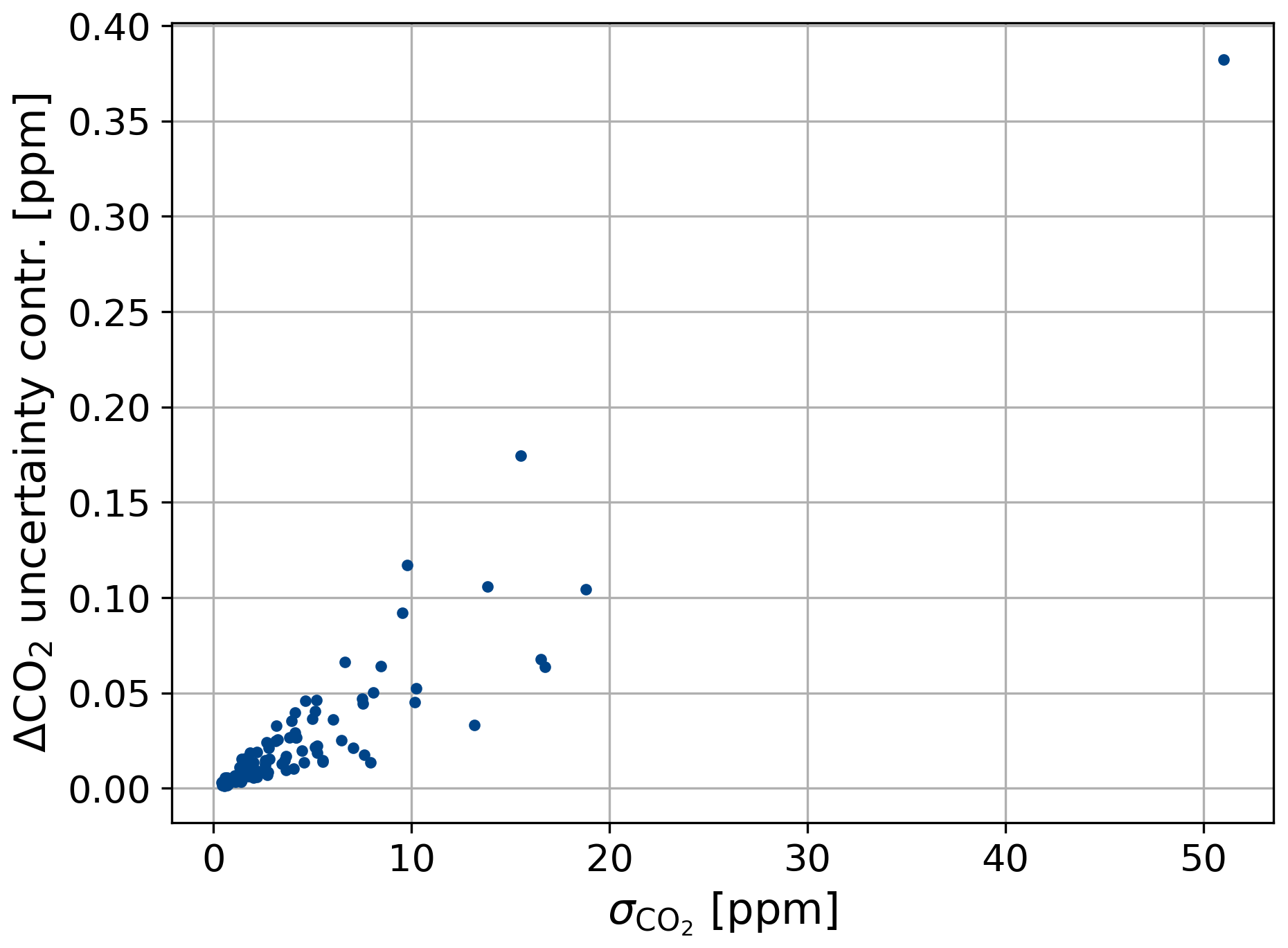
Figure C1 Estimated ΔCO₂ uncertainty contribution due to a variability in the sampling flow rate as a function of the standard deviation ${\mathit{\sigma }}_{{\mathrm{CO}}_{\mathrm{2}}}$ of CO₂ of the ambient air during the sampling periods of the 103 REA Zurich samples.

Appendix D: ΔffCO₂ uncertainties

As mentioned in Sect. 3, ${\mathrm{\Delta }}_{\mathrm{photo}}^{\mathrm{14}}$, ${\mathrm{\Delta }}_{\mathrm{nf}}^{\mathrm{14}}$, and Δc_nf = $(c_{\mathrm{nf}}^{\uparrow }-c_{\mathrm{nf}}^{\downarrow })$, which are needed to calculate ΔffCO₂, are not known but are estimated as given in Table 1. To illustrate the effects of each variable on the final ΔffCO₂ estimate, Fig. D1 shows the differences between ΔffCO₂ calculated using the values in Table 1 and ΔffCO₂ when one of the variables is changed. For the latter calculation, values over the maximum plausible range (based on ${\mathrm{\Delta }}_{\mathrm{meas}}^{\mathrm{14}}$ and Δc_meas) and uncertainties close to mean measurement uncertainties were chosen (2 ‰ for ${\mathrm{\Delta }}_{\mathrm{nf}}^{\mathrm{14}}$ and ${\mathrm{\Delta }}_{\mathrm{photo}}^{\mathrm{14}}$ and 1 ppm for Δc_nf). Therefore, Δ(ΔffCO₂) plotted on the y axes represents the absolute error that would be made with the current assumptions if the “true” values were those given on the x axes.

For all samples, higher ${\mathrm{\Delta }}_{\mathrm{nf}}^{\mathrm{14}}$ and Δc_nf lead to higher ΔffCO₂ estimates. Consequently, with the assumptions of ${\mathrm{\Delta }}_{\mathrm{nf}}^{\mathrm{14}}$ = 9 ± 16 ‰ and Δc_nf = 5 ± 5 ppm, ΔffCO₂ would be overestimated or underestimated if the actual values were smaller or larger. The magnitude of the effect depends on the difference ${\mathrm{\Delta }}_{\mathrm{nf}}^{\mathrm{14}}-{\mathrm{\Delta }}_{\mathrm{photo}}^{\mathrm{14}}$ and is therefore largest for winter samples.

The effect of ${\mathrm{\Delta }}_{\mathrm{photo}}^{\mathrm{14}}$ is sample-specific because the reference values are different for each sample. However, for most samples, ΔffCO₂ decreases with increasing ${\mathrm{\Delta }}_{\mathrm{photo}}^{\mathrm{14}}$.

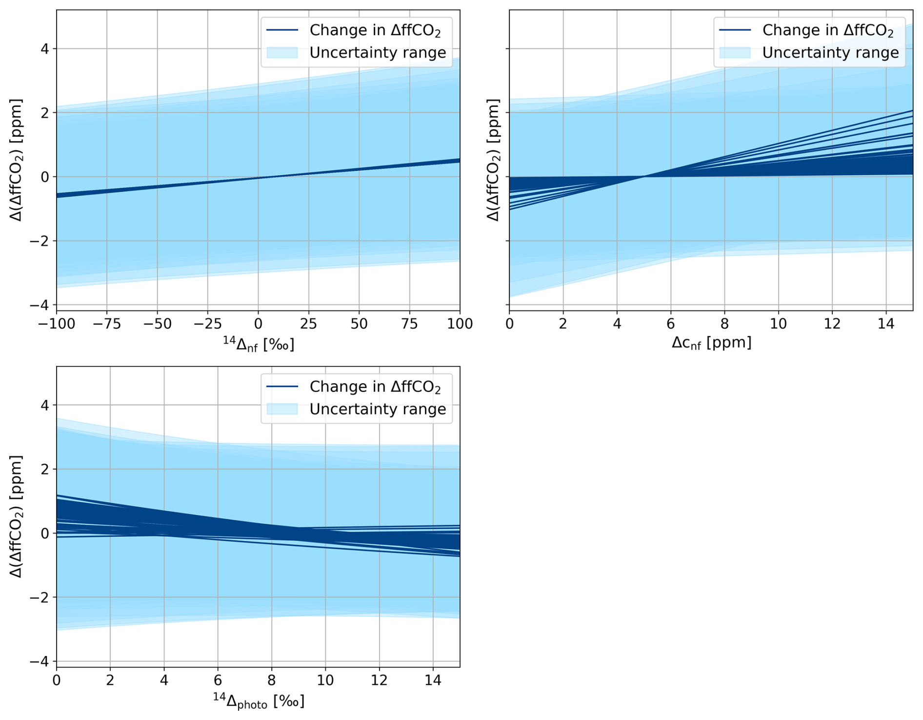
Figure D1 Impact of different assumptions for Δ¹⁴ values of CO₂ differences between up and down flasks due to respiration and biofuels (non-fossil, nf) and photosynthesis (photo) and the non-fossil signal Δc_nf = $c_{\mathrm{nf}}^{\uparrow }-c_{\mathrm{nf}}^{\downarrow }$ based on estimates of ΔffCO₂ = $c_{\mathrm{ff}}^{\uparrow }-c_{\mathrm{ff}}^{\downarrow }$. For each REA sample, the difference in ΔffCO₂ with respect to the reference settings used in this study is shown, where ${\mathrm{\Delta }}_{\mathrm{nf}}^{\mathrm{14}}$ = 10 ± 16 ‰, Δc_nf = 5 ± 5 ppm, and ${\mathrm{\Delta }}_{\mathrm{photo}}^{\mathrm{14}}$ = $\mathrm{0.5}\cdot ({{\mathrm{\Delta }}_{\mathrm{meas}}^{\mathrm{14}}}^{\uparrow }+{{\mathrm{\Delta }}_{\mathrm{meas}}^{\mathrm{14}}}^{\downarrow })$ ± 10 ‰. The light-blue ribbons indicate the 1σ uncertainty range due to measurement uncertainties.

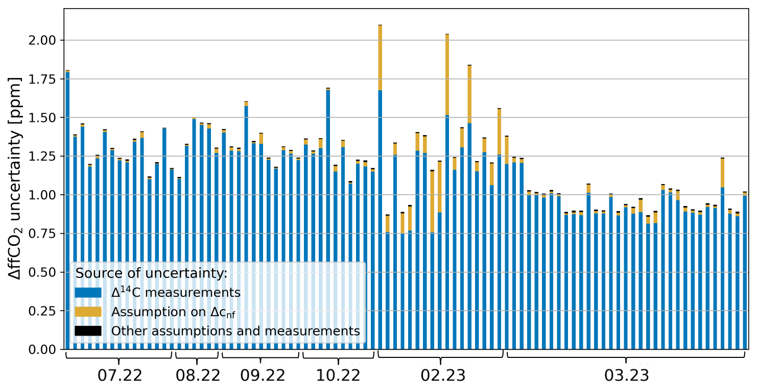
Figure D2 Contributions to the absolute uncertainty of ΔffCO₂ estimates (Eq. 9, with assumptions as given in Table 1) for each REA sample, collected between July 2022 and March 2023. Δ¹⁴ measurement uncertainties and an estimated non-fossil CO₂ difference between updraft and downdraft samples of 5 ± 5 ppm are the main contributors. The ΔCO₂ uncertainties due to the sampling process and the laboratory analysis, as well as the assumptions regarding the Δ¹⁴C signatures of photosynthesis, respiration, and biofuels (shown here in black), are negligible.

Varying the variables over the entire reasonable range, the differences can be as large as 2 ppm and thus of the same order of magnitude as ΔffCO₂ itself. Nevertheless, due to the large ¹⁴CO₂ measurement uncertainty (compare to light-blue area in Fig. D1), the deviations from the previous ΔffCO₂ estimates are not significant.

The fact that the uncertainty of ΔffCO₂ estimates is dominated by the ¹⁴CO₂ measurement uncertainty can also be seen in Fig. D2. It shows the contributions of each variable to the ΔffCO₂ uncertainty in ppm for each REA sample pair. The contributions of the ΔCO₂ uncertainty (including all aspects summarized in Table 3) and the assumptions regarding ${\mathrm{\Delta }}_{\mathrm{nf}}^{\mathrm{14}}$ and ${\mathrm{\Delta }}_{\mathrm{photo}}^{\mathrm{14}}$ are summarized as “other assumptions and measurements” (black) and are negligible for all samples. As discussed before, the impact of Δc_nf (orange) is especially large for the winter samples but is still secondary compared to the Δ¹⁴ measurement uncertainty (blue). The latter has been reduced from approximately 1.3 to 1.0 ppm as the graphite targets were measured with a new accelerator mass spectrometer starting January 2023. This improved the mean Δ¹⁴ precision from 2.1 ± 0.3 ‰ to 1.6 ± 0.2 ‰. Overall, the analyses show that the choice of ${\mathrm{\Delta }}_{\mathrm{photo}}^{\mathrm{14}}$, ${\mathrm{\Delta }}_{\mathrm{nf}}^{\mathrm{14}}$, and Δc_nf has little effect on the ΔffCO₂ estimate due to the current Δ¹⁴ measurement precision.