Interlaboratory comparison of continuous flow analysis (CFA) systems for high-resolution water isotope measurements in ice cores

The continuous flow analysis technique coupled with cavity ring-down spectrometry (CFA-CRDS) provides a method for high-resolution water isotope analysis of ice cores, which is essential for paleoclimatic reconstructions of local temperatures and regional atmospheric circulation. Compared to the traditional discrete method, CFA-CRDS significantly reduces analysis time. However, the effective resolution at which the isotopic signal can be retrieved from continuous measurements is influenced by system-induced mixing, which smooths the isotopic signal, and by measurement noise, which can further limit the resolution of the continuous record, introducing random fluctuations into the instrument's signal output. This study compares three CFA-CRDS systems developed at Ca' Foscari University (Venice), the Laboratoire des Sciences du Climat et de l'Environnement (Paris), and the Institut des Géosciences de l'Environnement (Grenoble) for firn core analysis. Continuous results are compared with discrete data to highlight the strengths and limitations of each system. A spectral analysis is also performed to quantify the impact of internal mixing on signal integrity and to determine the frequency limits imposed by measurement noise. These findings establish the effective resolution limits for retrieving isotopic signals from firn cores. Finally, we discuss critical system configurations and procedural optimisations that enhance the accuracy and resolution of water isotope analysis in ice cores.

1 Introduction

Water isotopes are valuable proxies for studying past climatic processes, providing insights into local temperature and atmospheric circulation patterns (Dansgaard, 1964; Petit et al., 1999). In permanently frozen regions of Antarctica, the glacial ice sampled through ice coring serves as a continuous archive of past climate conditions, with annual snowfall creating new layers at the top of the ice sheet every year. Low-accumulation areas like the East Antarctic Plateau (20–75 mm w.e. yr⁻¹; Wesche et al., 2016; Landais et al., 2017) often yield records with decadal or multi-decadal resolution (Petit, 1982; Casado et al., 2020). By contrast, in high-accumulation areas (100–300 mm w.e. yr⁻¹), such as in coastal regions in East Antarctica and West Antarctica, ice core records can achieve seasonal or annual resolution (Alley, 2000; Sigl et al., 2016; Markle et al., 2017). Depositional processes, such as precipitation intermittency (Steig, 1994; Laepple et al., 2011; Casado et al., 2020), introduce bias into the snow layers' recorded signal. In addition, post-depositional processes, including wind-driven snow redistribution (Picard et al., 2019), sublimation, and condensation, introduce stratigraphic noise into the snow's surface composition and alter local surface values (Casado et al., 2021; Wahl et al., 2022). Meanwhile, isotopic composition below the surface can be modified over time through processes like diffusion (Genthon et al., 2017). The deformation of deeper ice layers under the weight of the ice sheet compresses the timescale retrieved from each centimetre of ice analysed (Huybrechts et al., 2007). Therefore, high-resolution analyses are critical for ice cores to preserve the integrity of the isotopic signal. While deep ice cores from low-accumulation areas are traditionally analysed using discrete sampling, with resolutions ranging from 10 to 50 cm (Landais and Stenni, 2021; Grisart et al., 2022), a higher resolution (< 10 cm) is achieved in cores from high-accumulation areas, where seasonal signal can be detected (Goursaud et al., 2017; Crotti et al., 2021). In both cases, although precise, this method is time-consuming due to the extensive sample preparation and the need for offline analysis. In contrast, continuous flow analysis (CFA) coupled with a cavity ring-down spectrometry (CRDS) has emerged as a more efficient alternative, enabling high-resolution measurements of water isotopes (Gkinis et al., 2010). This system slowly and continuously melts solid ice sticks at the base, with the resulting liquid water being directed into a vaporiser before being injected into a CRDS instrument – typically a Picarro-brand isotopic analyser. This method eliminates the need for manual sample handling, significantly reducing analysis time. For instance, within the East Antarctic International Ice Sheet Traverse (EAIIST; Traversa et al., 2023) project, the analysis of 18 firn cores collected on the Antarctic Plateau (total length of about 960 m) would result in the analysis of approximately 20 000 samples at resolution of 5 cm. This would take more than 2 years of discrete analysis if conducted with a single CRDS instrument. In contrast, with CFA-CRDS, operating at a melt rate of 2.5–3 cm min⁻¹, the same analysis can be completed in roughly 3 months, with the capability to process up to 10 m of ice core per day. Additionally, the CFA offers the great advantage of providing – in parallel to the line for isotopic analysis – a non-contaminated innermost meltwater flow for further analysis. The innermost meltwater flow is used for direct measurement, such as chemical analysis (trace elements, heavy metals, biomass burning tracers, etc.) and insoluble particle volume and distribution, and is simultaneously collected as discrete aliquots, greatly reducing the need for decontamination procedures in clean rooms. Despite its advantages, CFA-CRDS faces some technical limitations for isotopic analysis, one being the mixing of water molecules within the system, leading to signal smoothing (Gkinis et al., 2011). We use the term “mixing”, following the definition of Jones et al. (2017a), for all of the smoothing effects on the signal that occur within the CFA-CRDS system, including mixing occurring from the melt head to the instrument cavity. Mixing may decrease the signal amplitude. On the other hand, we refer to “diffusion” for all of the attenuation processes that happen naturally with in the firn (Gkinis et al., 2021). Overall, the transfer function of both processes follows the same equation (Eq. 1), but the length is usually longer for diffusion. The mixing length, influenced by the technical setup and variations in core section density at the melt-head stage due to capillary action, can differ significantly between systems. Consequently, isotopic values must be averaged over a depth interval equivalent to the mixing length to ensure accurate representation of the preserved climatic signal within the cores (Gkinis et al., 2011; Jones et al., 2017a). Additionally, measurement noise – referring to random fluctuations in the instrument signal output – further limits the effective resolution, restricting the ability to retrieve meaningful climatic signals at high frequencies.

In this study, we present the 4 m section of the firn PALEO2 core (EAIIST), analysed at three research institutes: Ca' Foscari University in collaboration with the Institute of Polar Science, National Research Council (ISP-UNIVE, Venice, Italy); the Laboratoire des Sciences du Climat et de l'Environnement (LSCE, Paris, France); and the Institut des Géosciences de l'Environnement (IGE, Grenoble, France). These laboratories collaborate on international ice core projects such as EAIIST and Beyond EPICA Oldest Ice Core (BE-OIC – Parrenin et al., 2017; Lilien et al., 2021) and share common samples, emphasising the need for accurate comparisons between the different systems. We compared CFA results with discrete profiles at 1.5 cm resolution to highlight the strengths and limitations of each technical setup and operating procedure. Power spectral density (PSD) analysis is used to quantify the effects of mixing on the signal and to determine the maximum resolution achievable by each system, as constrained by internal mixing and measurement noise.

2 Methods

2.1 Ice core processing

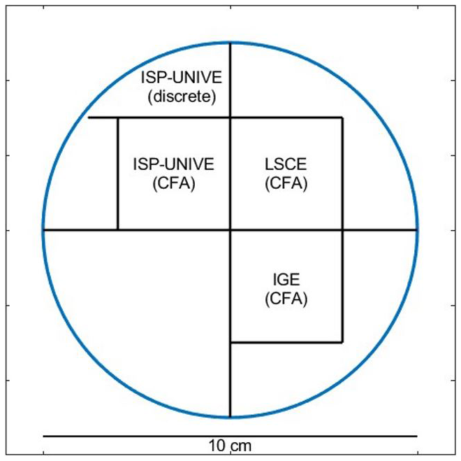
Four ice cores were drilled at the PALEO site (79°64^′ S, 126°13^′ E; borehole temperature: −46.5 °C) during the EAIIST on the Antarctic Plateau (Traversa et al., 2023). In this study, we focus on the PALEO2 firn core (18 m deep) to compare three CFA-CRDS systems. The full core was continuously analysed at LSCE in June 2023, while 4 m sections (12–16 m depth) were analysed at IGE in July 2023 and at ISP-UNIVE in January 2024. This 4 m interval, with an average density of ∼ 0.58 g cm⁻³, was selected to explore the performance of the systems on low-density firn while maintaining sufficient structural integrity for handling and analysis in the cold room. The core was cut into about 1.00 × 0.03 × 0.03 m sticks (Fig. 1). During the preparation of the ice sticks for the ISP-UNIVE measurements, discrete samples of 1.5 cm length were also cut. However, due to sample loss during the cutting process and uncertainties associated with manual cutting, the discrete samples resulted in a final resolution of 1.7 cm on average. The samples were stored frozen in PTFE bottles and analysed offline. Spectral analyses show that no significant diffusion occurred during the 6-month storage at −20 °C between the two cutting sessions. The comparison between the spectra will be presented in Sect. 3.5 and in Fig. 8. The remaining quarter of the core was stored in plastic bags for any future investigation.

Figure 1 Cutting scheme of PALEO2 core for CFA-CRDS systems and discrete sampling.

2.2 Isotopic measurements and data calibration

Here, the isotope values of δD and δ¹⁸O are reported as the deviation of the ratio of heavy to light isotopes relative to the Vienna Standard Mean Ocean Water (V-SMOW – Table 1a) international standard, where δ values are expressed in parts per mil (‰):

$$\mathit{\delta }=\left({\displaystyle \frac{R_{\mathrm{SAMPLE}}}{R_{\mathrm{VSMOW}}}}-\mathrm{1}\right),$$

where R_SAMPLE and R_VSMOW are the ratios between ¹⁸O $/$ ¹⁶O or D $/$ H in the sample and in V-SMOW, respectively. The second-order parameter deuterium excess (dxs) is defined as follows (Craig, 1963; Dansgaard, 1964):

$$\mathrm{dxs}=\mathit{\delta }\mathrm{D}-\mathrm{8}\times {\mathit{\delta }}^{\mathrm{18}}\mathrm{O}.$$

All reported isotope values are calibrated against the internal laboratory standards (STDs) provided by each institute, which are, in turn, calibrated against the international reference waters of V-SMOW (Vienna Standard Mean Ocean Water – Table 1a) and SLAP (Standard Light Antarctic Precipitation – Table 1a). Calibration involves applying a linear regression between the “measured” and “known” values of STDs, using the resulting slope and intercept to correct the sample data to the reference scale. STDs have isotopic compositions similar to those expected for Antarctic ice cores (Landais and Stenni, 2021) to minimise the instrument's memory effect and accurately capture the highly negative isotopic values typical of polar snow.

Table 1 Isotopic values (‰) of (a) the international standards V-SMOW and SLAP and (b) ISP-UNIVE, (c) LSCE, and (d) IGE internal laboratory standards used for calibration.

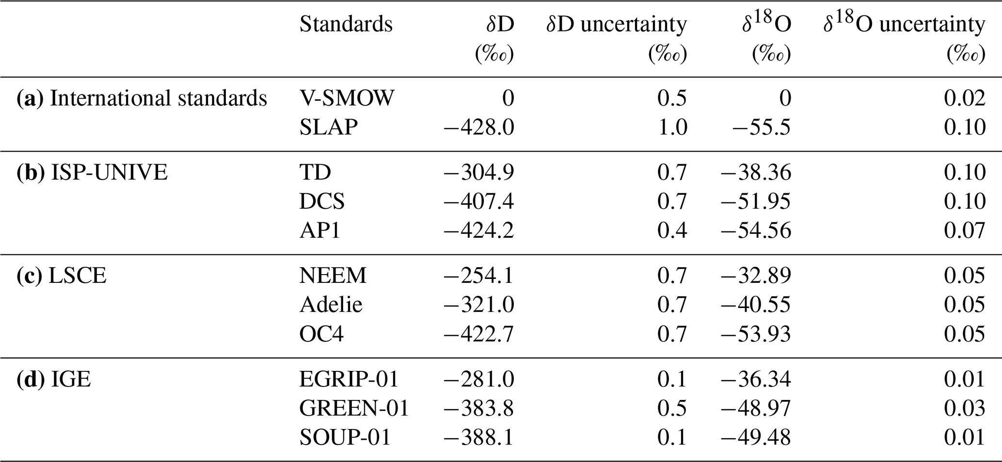
The discrete samples were analysed at ISP-UNIVE using a Picarro L2140-i. The standards TD (Talos Dome) and AP1 (Antarctic Plateau 1) were used for calibration, while two vials of DCS (Dome C Snow) were analysed as controls (Table 1b). The accuracy of offline measurements was determined as the mean difference between the control and true values of the STD controls, with uncertainty being represented by their standard deviation (SD). This yielded accuracies of −0.01 ‰ for δ¹⁸O, −0.07 ‰ for δD, and −0.02 ‰ for d excess, with corresponding uncertainties of ±0.07 ‰, ±0.4 ‰, and ±0.4 ‰, respectively.

The continuous analyses were conducted using the three CFA systems coupled with CRDS Picarro-brand isotopic analysers: the L2130-i model at ISP-UNIVE and LSCE and the L2140-i model at IGE. Continuous raw data are calibrated by injecting water STDs at a constant humidity level before and/or after each daily measurement. From each calibration standard injection, only a data interval with stable humidity is selected. At the ISP-UNIVE laboratory, standards AP1 and DCS (Table 1b) are injected for 20 min, with the final 5 min being used for analysis. At LSCE, the standards NEEM, Adélie, and OC4 (Table 1c) are injected for 25 min, and the final 3 min are selected. At IGE, the standards EDC, EGRIP-01, and SOUP-01 (Table 1d) are injected for 10 min, and a 3 min interval with stable humidity is chosen. At ISP-UNIVE, STDs are measured at the start of the day, while, at LSCE and IGE, STDs are measured at both the beginning and the end of the analysis. At LSCE, three calibration methods – using the start day, the end day, or the average of both – were tested, showing no significant measurement drift throughout the day.

2.3 CFA-CRDS coupled system

The CFA-CRDS systems are commonly composed of three main units (Jones et al., 2017a): the ice-core-melting component located in a cold room, which generates a continuous stream of liquid water (Fig. 2 – blue block); a vaporiser that converts the liquid into vapour (Fig. 2 – yellow block); and the CRDS isotopic analyser (Fig. 2 – green block). This setup enables online water isotope measurements of δD and δ¹⁸O during the melting of the cores, which are cut into sticks and are loaded vertically above the melt head (MH). The transport line typically includes a debubbler, which permits the release of air bubbles from the water stream as it passes through. A selector valve (SV) prior to the vaporiser allows for switching between the CFA line, ultrapure water (UPW), and calibration STDs. The water vapour is transported from the vaporiser into the analyser using a carrier gas (N2 or zero air). The key differences between the three laboratories are summarised in Table 2 and Fig. 2. The novel ISP-UNIVE-CFA system is highly scalable according to the specific laboratory needs (Barbaro et al., 2022; Spagnesi et al., 2023). A conductivity device monitors the meltwater stream before it enters the small-volume 200 µL triangular flat-cell debubbler. The debubbler has one inlet and two outlets: one for the debubbler meltwater and the other, connected to the waste, for the air bubbles and excess meltwater (∼ 0.22 mL min⁻¹). The LSCE-CFA system features a low-dead-volume glass debubbler with a volume of 430 µL, regulated by an automatic flow control to prevent overflow. The system includes a dust filter (A-107 IDEX stainless-steel filter, 10 µm) and three conductivity devices. The IGE-CFA system supports a broader range of online analyses and includes a 1000 µL low-dead-volume glass debubbler. Flow is manually regulated via pump adjustment, and the debubbler is connected to an open line and continuously monitored. Meltwater passes through a 180 µm dust filter and a longer distribution line. The isotopic line includes an additional 20 µm filter and a conductivity device prior to the analyser.

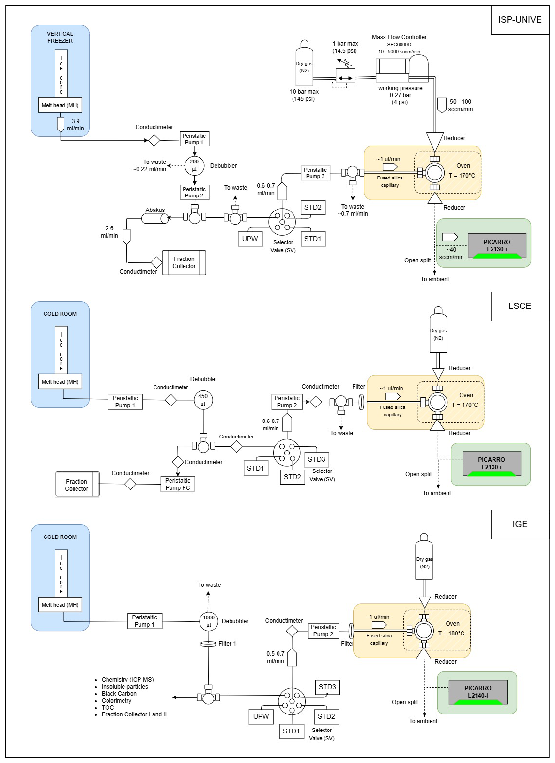
Figure 2 Schematic of the CFA-CRDS systems. The ice-core-melting component, the vaporiser, and the isotopic analyser are highlighted in blue, yellow, and green, respectively.

Table 2 Technical properties of different CFA-CRDS setups.

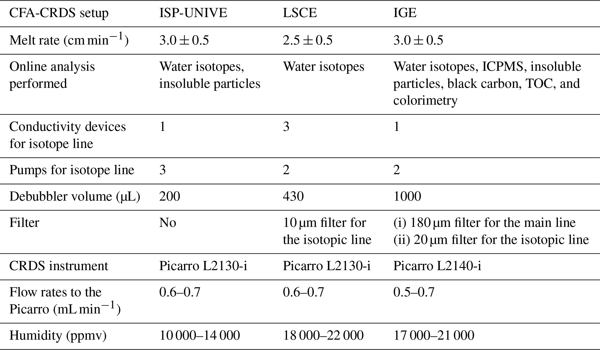
The three melt heads used are similar, featuring a square cross-section with an inner and outer collection area separated by a 2 mm high triangular ridge, as with the one described by Bigler et al. (2011). All three of the vaporisers are similar and inspired by the capillary-based system described by Gkinis et al. (2010). LSCE and IGE vaporisers were both designed at the Paris laboratory, while the ISP-UNIVE one was built at Ca' Foscari University of Venice. The stream is split from the incoming stream into a 50 µm inner diameter fused-silica capillary, and the rest goes into the waste line. The split takes place in a T split with a bore diameter of 0.5 mm. The sample micro-flow is injected into the oven (170 °C at ISP-UNIVE and LSCE and 180 °C at IGE), where it vaporises and mixes with dry air or nitrogen. At ISP-UNIVE, a mass flow controller (Sensirion AG SFC6000D) is used to control the dry air. The humidity levels at which the continuous analyses are performed are as follows: 10 000–14 000, 18 000–22 000, and 17 000–21 000 ppmv, respectively, for ISP-UNIVE, LSCE, and IGE. The lower range maintained by ISP-UNIVE represents the maximum level achievable with the nominal setup, balancing melting speed, discrete sample collection via the fraction collector, online measurement, and the requirement to supply a constant water volume to the CRDS instrument. In general, we do not aim here to isolate the specific impact of each individual system component as this is beyond the scope of the present study. Rather, we provide a general overview of the factors that may contribute to mixing within the main liquid or vapour phases of the systems.

2.4 Mixing in the CFA systems

The mixing in the CFA system attenuates the original signal preserved in the firn and/or ice cores, resulting in a smoothing of the isotope record (Gkinis et al., 2011). This effect, analogous to vapour diffusion processes occurring naturally in the firn, arises from the displacement of water molecules from their original relative positions in the ice matrix. However, a key distinction between CFA mixing and firn diffusion lies in their respective typical lengths: while firn diffusion typically acts at orders of 6–8 cm (Johnsen et al., 2000), mixing is expected to occur over 0.7–1.5 cm (Gkinis et al., 2011; Jones et al., 2017a). Mixing occurs at multiple stages in the CFA setup, including at the melt head due to water capillarity flow within the porous firn, in the debubbler, within the vaporiser chamber and CRDS cavity, and along the transport tubing in both the liquid and vapour phases (Jones et al., 2017a). We assess the mixing effect occurring throughout the CFA systems and disentangle the main contributions in the phase upstream and downstream of the selector valve. Two different impulse responses are evaluated. The first step function, generated at the melt-head stage (MH), involves the melting of two ice sticks in a row with different isotopic compositions. The second step function includes the mixing downstream of the selector valve (SV) by switching between two isotopically distinct liquid samples. The impulse response is determined by fitting a probability density function (PDF) over the first derivative of the Picarro response, described by the normal Gaussian, as suggested by Jones et al. (2017a) (Eq. 1):

$$\begin{array}{}\text{(1)}& f\left(x\right)=a_{\mathrm{1}}\times \exp \left(-{\left({\displaystyle \frac{x-b_{\mathrm{1}}}{c_{\mathrm{1}}}}\right)}^{\mathrm{2}}\right),\end{array}$$

where a₁ is the amplitude, b₁ is the mean, and c₁ is the standard deviation of the curve. Mixing lengths (σ) are defined as follows (Eq. 2):

$$\begin{array}{}\text{(2)}& \mathit{\sigma }={\displaystyle \frac{c_{\mathrm{1}}}{\sqrt{\mathrm{2}}}}.\end{array}$$

The σ_MH reflects the mixing of the entire CFA system, whereas the σ_SV represents the mixing downstream of the SV. The latter includes the mixing caused by the presence of a peristaltic pump common to all three of the systems and a mixing related to a filter prior the vaporiser for LSCE and IGE (Fig. 2). To estimate mixing length upstream of the SV, referred to as σ_L, we calculate the root square of the quadrature difference between σ_MH and σ_SV (Jones et al., 2017a).

Previous studies used mock ice with varying isotope compositions to calculate σ_MH (Jones et al., 2017a; Dallmayr et al., 2025). In this study, we analyse the PALEO2 firn core (ρ = 0.58 g cm⁻³), which has a lower density and higher porosity compared to artificial ice (ρ = 0.92 g cm⁻³). To assess the unavailability of ultrapure water (UPW) mock sticks with firn-like density, the σ_MH values calculated in this study are based on tests involving different firn and/or ice transitions. Specifically, a mean value derived from ice-to-ice, ice-to-firn, and firn-to-ice transitions is considered to be the best laboratory-based approximation of the effective mixing length. We note that the results obtained may differ for deeper and denser ice core sections due to capillary effects. While diffusivity at the melt head is generally expected to be lower in denser ice due to reduced porosity, the transition from firn to ice is also influenced by changes in melt-head temperature and melt rate, which should be taken into account.

2.5 Data processing

The isotopic raw data from the Picarro analyser, provided at an acquisition time of ∼ 1 s, are calibrated according to the V-SMOW and SLAP and then are post-processed. The post-processing includes (i) converting the time to depth scale, (ii) filtering data affected by memory effects and artefacts, and (iii) custom block averaging the data at a resolution of 0.5 cm.

(i) The depth scale for the isotopic record is built through two common computational steps across all three laboratories. First, the timescale at MH is converted to depth using the measured ice stick lengths and the continuous recording of the encoder position. The encoder (located at the top of the ice sticks) records the melting of the cores at a frequency of ∼ 1 Hz. Second, the arrival time at the CRDS, conductivity cell, and fractionation collectors is calculated based on the peristaltic pump flow rates. At ISP-UNIVE and IGE, the MH-to-CRDS delay is estimated through preliminary tests and is corrected for pump rate changes. At LSCE, the MH-to-CRDS time for the liquid phase is calculated using the continuously recorded flow rates and the volumes associated with each component of the CFA setup. Additionally, the delay time for gas-phase transport to the CRDS is estimated based on isotopic steps from the SV under standard operating conditions (specifically, N2 and water flow rates). This gas-phase delay is assumed to remain constant throughout the duration of the CFA run.

Conductivity profiles plotted on the common depth scale help to validate the processing. For LSCE, validation is based on the effective synchronisation of three conductivity profiles. At IGE, where a single device is located prior to the isotopic analyser, validation relies on aligning conductivity peaks – which correspond to transitions between individual ice sticks – with logged depths. Lastly, adjustments may be required between the actual stick length and the depth logged in the field, particularly for fragile and crumbling firn cores. Temporary blockages or stick collapses can introduce uncertainties when assigning depth to the isotopic profile. Whenever possible, such events should be documented and considered during the interpretation of the depth profiles. (ii) Data at the beginning and end of CFA runs that are affected by mixing with pre- and post-circulated water are manually removed. At ISP-UNIVE, humidity drops – well below the typical working condition – are manually selected using a MATLAB graphical user interface and substituted with linearly interpolated values or removed when the depth intervals exceed 10 cm. (iii) Eventually, data are custom block averaged at a resolution of 0.5 cm.

2.6 Continuous and discrete isotopic record comparison

The comparison between continuous and discrete isotopic records aims to highlight key technical differences in the CFA-CRDS setups and the operating procedures. Comparisons of profiles versus depth assess the agreement in terms of calibration and depth scale attribution between laboratories. Additionally, the power spectral density (PSD) analysis – defined as the measure of a signal's power content in the frequency domain – reveals system limitations caused by mixing and measurement noise. Before presenting the comparison in Sect. 3, we briefly introduce the PSD approach (Fig. 3), providing an idea of the mixing and measurement noise effects in the continuously measured signal. For this purpose, we consider, ideally, the discrete record as the best available approximation of the true signal preserved in the ice, limited only by a discrete sampling resolution and uncertainties in the depth for the sampling cut. The discrete spectrum shows a “flat” shape at frequencies around 100 m⁻¹ (white area), where the signal is dominated by precipitation intermittency and stratigraphic noise (Laepple et al., 2018; Casado et al., 2020). At these frequencies, the observed variability arises from random processes rather than from climatic trends or seasonal signals. In contrast, attenuation begins at 50 cm⁻¹ (yellow area), consistently with diffusion effects (Johnsen et al., 2000). For the 12–16 m depth section of cores collected on the Antarctic Plateau, such as the PALEO2 core (density of ∼ 0.58 g cm⁻³), firn diffusion is estimated by previous studies to have a length of 6–8 cm for δ¹⁸O (Whillans and Grootes, 1985; Laepple et al., 2018; Johnsen et al., 2000). The diffusion effect can be modelled by the following equation (Johnsen et al., 2000):

$$\begin{array}{}\text{(3)}& P=P_{\mathrm{0}}\exp \left(-k^{\mathrm{2}}{\mathit{\sigma }}_{\mathrm{diff}}^{\mathrm{2}}\right),\end{array}$$

where σ_diff represents the firn diffusion length, and k=2πf, with f being the frequency.

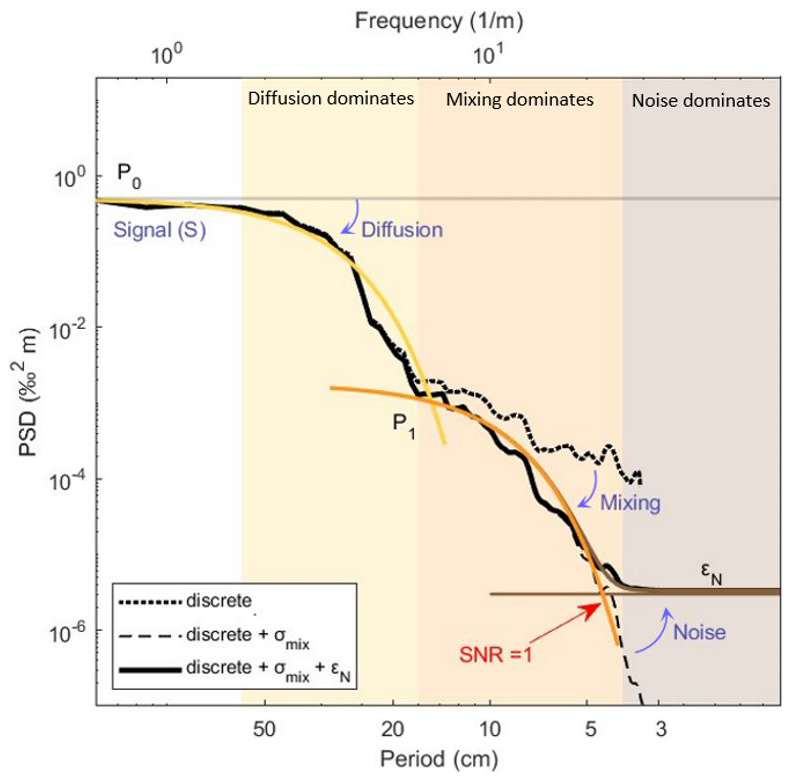
Figure 3 Schematic PSD of discrete and simulated profiles. The simulated spectrum (solid black line) is obtained by combining the discrete power density (dashed black line) affected by natural diffusion in the firn (σ_diff – yellow) with the mixing effect occurring in the CFA system (σ_mix – orange) and the measurement noise associated with continuous measurements (ε_N – brown).

At higher frequencies (∼ 3–20 cm⁻¹), a signal power is still observed. This noise likely arises in parallel with or after diffusion processes and can probably be related to stratigraphic or other post-depositional processes. Indeed, we note that this spectral feature is preserved in both discrete and CFA records, and it appears to be attenuated in the latter due to signal mixing. However, the origin mechanism of this spectral power remains unclear, and a comprehensive investigation of this phenomenon lies beyond the scope of the present study. Here, we aim to use the discrete dataset – resampled at 0.5 cm resolution to match the post-processed resolution of the continuous record – as a reference signal to which mixing and measurement noise are applied. To this end, we apply an additional Gaussian smoothing to account for the CFA mixing length (σ_mix) and incorporate the measurement noise (ε_N) determined for the online analysis, as described by the following equation (Eq. 4):

$$\begin{array}{}\text{(4)}& P=P_{\mathrm{1}}\exp \left(-k^{\mathrm{2}}{\mathit{\sigma }}_{\mathrm{mix}}^{\mathrm{2}}\right)+{\mathit{\epsilon }}_{\mathrm{N}}.\end{array}$$

As a result, the simulated spectrum diverges from the discrete spectrum at the frequency where CFA mixing begins to affect the signal, showing smoothing in the medium-frequency range (> 0.5 m⁻¹, orange area) and flattening at higher frequencies due to measurement noise (brown area). Measurement noise generates a flat spectrum at the frequency where the signal-to-noise ratio (SNR) equals 1 (Casado et al., 2020), permitting us to determine the frequency limit where meaningful climatic information can still be retrieved as the point where the spectra of signal and noise intersect. Beyond this limit, noise dominates the signal as the correlation between the record and the signal is defined as (Eq. 5)

$$\begin{array}{}\text{(5)}& r^{\mathrm{2}}={\displaystyle \frac{\mathrm{SNR}}{\mathrm{1}+\mathrm{SNR}}}.\end{array}$$

At SNR = 1, a minimum significant correlation $r=\sqrt{\mathrm{0.5}}\sim \mathrm{0.71}$ is reached. A similar behaviour is expected for the power spectral densities (PSDs) of the continuous records, allowing us to identify the maximum reliable frequency retained in the signal.

3 Results

In this section, we compare the measurements of the same 4 m section of the PALEO2 firn core by the CFA setups of ISP-UNIVE, LSCE, and IGE with the discrete results. By analysing in both the depth and spectral domains, we evaluate the precision and accuracy of each setup and operational procedure. In turn, we assess the effective resolution limit at which a reliable isotopic signal can be retrieved from the CFA outputs, based on each system's internal mixing and measurement noise.

3.1 Continuous measurements noise

To assess the stability and noise of the combined vaporiser and CRDS analyser, we calculate the Allan variance (Allan, 1966) of isotopic time series (an example of the ISP-UNIVE time series is presented in Fig. B1 in Appendix B). The time series are continuous measurements of UPW under constant humidity conditions that match those of CFA-CRDS analyses. The Allan variance is computed by taking a time series of size N. The data are divided into m non-overlapping intervals, each containing $k=N/m$ data points. The acquisition time per data point is t_i; thus, the integration time for each interval is ${\mathit{\tau }}_m=k\cdot t_i$. The Allan variance for a given τ_m is defined as follows (Eq. 6):

$$\begin{array}{}\text{(6)}& {\mathit{\sigma }}^{\mathrm{2}}\left({\mathit{\tau }}_m\right)={\displaystyle \frac{\mathrm{1}}{\mathrm{2}m}}\sum _{j=\mathrm{1}}^m{\left({\stackrel{\mathrm{‾}}{\mathit{\delta }}}_{j+\mathrm{1}}-{\stackrel{\mathrm{‾}}{\mathit{\delta }}}_j\right)}^{\mathrm{2}},\end{array}$$

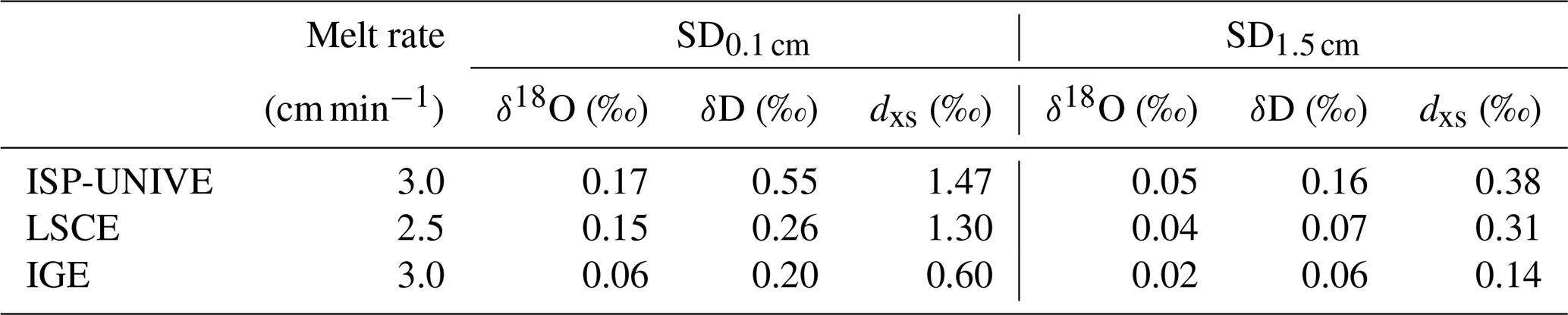
where ${\stackrel{\mathrm{‾}}{\mathit{\delta }}}_{j+\mathrm{1}}$ and ${\stackrel{\mathrm{‾}}{\mathit{\delta }}}_j$ are the mean values of neighbouring non-overlapping intervals j and j+1. This method quantifies the time-dependent variance between consecutive intervals, making it particularly suitable for evaluating noise and drift in high-resolution continuous measurements. The calculation is based on continuous UPW flow into the CRDS analyser under stable humidity conditions (Fig. 4, Table 3). For ISP-UNIVE, LSCE, and IGE, the mixing ratios are ∼ 14 800, ∼ 20 000, and ∼ 18 100 ppmv, respectively. For ISP-UNIVE and LSCE, we selected 2 h of continuous data, while, for IGE, 1.5 h time series was used. The raw data, provided every 0.85 s for L2130-i models (ISP-UNIVE and LSCE) and every 0.72 s for the L2140-i model (IGE), are interpolated at 1 s post-acquisition. All systems show a decrease with a slope of $N^{-\mathrm{1}/\mathrm{2}}$, characteristic of white noise, for at least τ = 250 s, indicating that precision improves with longer integration times. For τ=2 s (corresponding to a melting of 0.1 cm of ice at 3.0 cm min⁻¹), the SD values for δ¹⁸O are 0.17 ‰ (ISP-UNIVE), 0.15 ‰ (LSCE), and 0.06 ‰ (IGE). At τ=30 s (time required to melt 1.5 cm of a sample), precision improves, with SDs decreasing to 0.05 ‰, 0.04 ‰, and 0.02 ‰, respectively. The Picarro L2140-i analyser used at IGE demonstrates higher precision than the L2130-i model used at LSCE despite operating at lower humidity levels during the Allan variance assessment. In addition, the L2130-i analyser at ISP-UNIVE shows a precision comparable to that at LSCE. These results suggest that precision and instrument noise are primarily determined by the analyser's intrinsic performance rather than the specific technical configuration of the CFA system. However, due to the considerable variability among Picarro instruments, a detailed explanation of the better performance of the L2140-i relative to the L2130-i lies beyond the scope of this study.

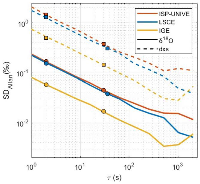
Figure 4 Allan variance computed from 1 h continuous UPW flow for ISP-UNIVE (orange, at 14.850 ± 53 ppmv), LSCE (blue, at 20.380 ± 190 ppmv), and IGE (yellow, at 18.100 ± 105 ppmv) for δ¹⁸O and d excess. The dots and squares indicate, for each system, the specific integration times (τ) needed to melt 0.1 and 1.5 cm, respectively, of the ice core at the nominal melting rate.

Table 3 Allan variance for δ¹⁸O, δD, and d excess with regard to the integration times (τ) needed to melt 0.1 and 1.5 cm of the ice core at the nominal melting rate for each institute.

3.2 Impact of the humidity level

The impact of humidity on the isotopic measurements was evaluated for the three water vapour mixing ratio ranges used during the analyses. The range maintained at ISP-UNIVE, between 10 000 and 14 000 ppmv, with occasional fluctuations down to 8000 ppmv, was assessed using the laboratory standard AP1, analysed in 5 min intervals at steps of 8000, 9500, 11 500, and 14 000 ppmv. For each step, the last 3 min were selected. The differences in δ¹⁸O and δD between these humidity levels were smaller than the Allan variance (see Sect. 3.1) for a 1 s integration time, corresponding to the resolution of the data Picarro output (Fig. 5). For the LSCE setup, the same approach was followed, with humidity steps performed between 17 000 and 23 000 ppmv. Overall, we calculate an impact of humidity levels on the average isotopic composition of 0.015 ‰ per 1000 ppmv and 0.216 ‰ per 1000 ppmv for δ¹⁸O and δD, respectively. Consequently, we opted not to apply humidity level correction to the data for the range within which the measurements were performed.

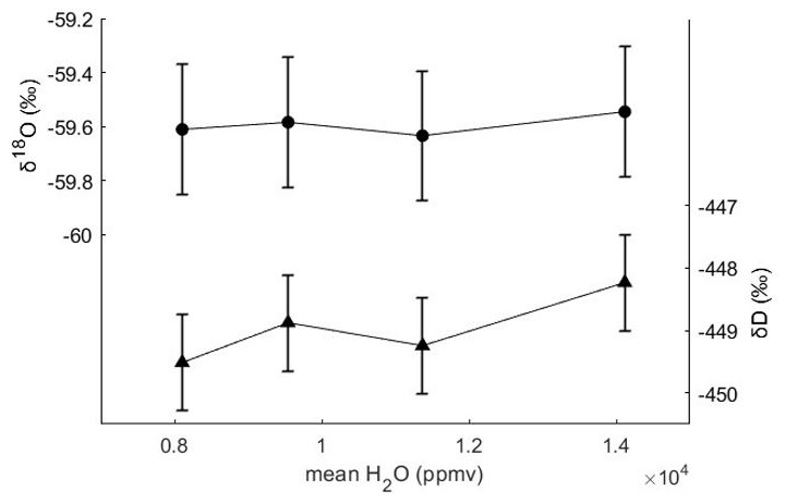
Figure 5 Mean δ¹⁸O and δD values for the 3 min intervals selected at humidity levels of 8000, 9500, 11 500, and 14 000 ppmv in the ISP-UNIVE setup. The confidence levels are defined as the Allan variation for an integration time of 1 s (±1σ).

Between 10 000 and 20 000 ppmv, the precision of the Picarro instrument at timescales comparable to those of the CFA remains relatively stable. This was assessed through an Allan variance analysis conducted across humidity levels in the 10 000–20 000 ppmv range (see Fig. A1 and Table A1 in Appendix A).

3.3 Evaluation of mixing lengths from impulse response

Here, we present the mixing lengths of the three systems, evaluated for the melt-head stage (MH), which reflects the total mixing within the CFA-CRDS systems, and for the selector valve stage (SV). The theoretical basis for these calculations is detailed in Sect. 2.4.

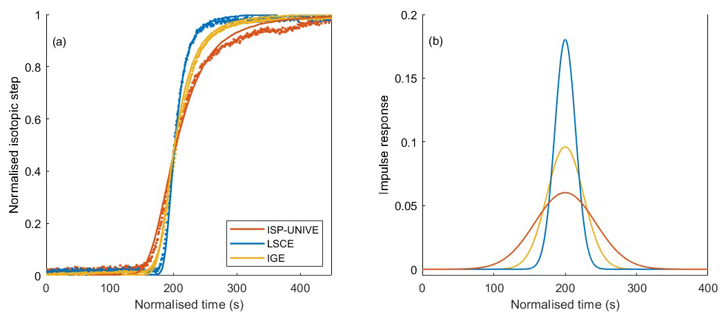
Figure 6 (a) Raw data interpolated at 1 s post-acquisition and respective normalised transfer function for ice steps at the stage of the CFA melt head for δ¹⁸O. (b) Normal PDF impulse response function. Firn-to-ice transitions are shown for ISP-UNIVE and LSCE, while an ice-to-firn transition is shown for IGE.

Due to the unavailability of a UPW mock stick with firn-like density, we tested different transition types: ice-to-firn, firn-to-ice, and ice-to-ice (Table C1 in Appendix C). Although the mixing lengths may vary depending on the density of the sticks during melting, this approach provides the best estimate within the given experimental constraints, even if the values may be slightly underestimated for the firn-to-firn case. Figure 6a shows an example of a normalised step function: firn-to-ice transitions are shown for ISP-UNIVE and LSCE, while an ice-to-firn transition is shown for IGE. Prior to normalisation, the isotopic difference between ice sticks at the MH (or liquid standards at SV) ranges from 40 ‰ to 50 ‰ for δ¹⁸O and from 380 ‰ to 400 ‰ for δD. The corresponding impulse responses are presented in Fig. 6b. The mixing lengths from the MH derived for each laboratory show no significant differences across transition types (Table C1). We therefore define σ_MH as the mean value of all transitions, which will correspond to σ_mix in the back-diffusion approach presented in the following sections.

Table 4 δ¹⁸O mixing lengths at melt-head stage (σ_MH) and at selector valve stage (σ_SV) for the three different CFA-CRDS systems. The mixing length in the liquid phase (σ_L) is calculated as the difference in quadrature between σ_MH and σ_SV. The mixing length expressed in seconds is converted into millimetres considering the average melting rate set at the three institutes. The 1SD values are given in parenthesis. The mixing lengths are compared with Jones et al. (2017a) at the Institute of Arctic and Alpine Research (INSTAAR) Stable Isotope Lab (SIL) and Dallmayr et al. (2025) at the Alfred-Wegener-Institut Helmholtz-Zentrum für Polar-und Meeresforschung (AWI).

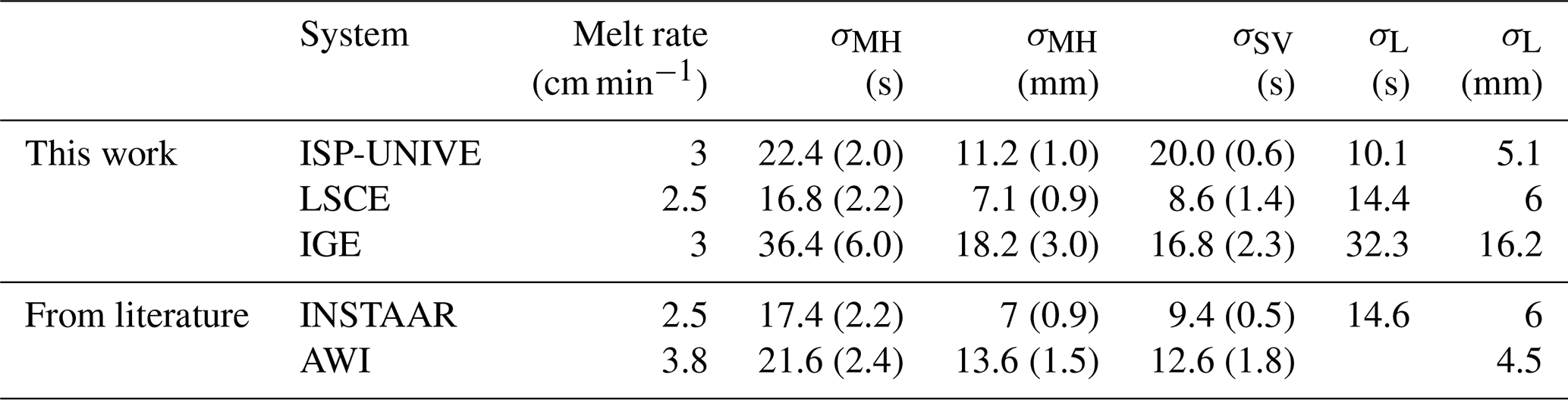
The mixing lengths (σ_MH, σ_SV, and σ_L) are summarised in Table 4. Since the values for δ¹⁸O and δD are very similar, we report only δ¹⁸O. The resulting mean σ_MH values are 7.1 mm for LSCE, 11.3 mm for ISP-UNIVE, and 18.2 mm for IGE. Values expressed in seconds are converted into millimetres using the average melting rate.

Overall, the LSCE system exhibits the smaller σ_MH, indicating the most efficient setup among the three systems evaluated. In contrast, IGE-CFA shows the highest σ_MH (Table C1), with the dominant contribution arising from mixing in the liquid phase, as reflected by the higher σ_L. This is likely due to the presence of a high-volume debubbler and a longer distribution line, required to accommodate the higher number of online measurements and discrete sampling operations performed by the laboratory. Notably, ISP-UNIVE shows more diffusion downstream of the selection valve (20.0 s) compared to upstream (10.1 s). This behaviour contrasts with the other systems presented in Table 4, including values for ice-to-ice transitions previously reported by Jones et al. (2017a) at the Institute of Arctic and Alpine Research (INSTAAR) Stable Isotope Lab (SIL) and by Dallmayr et al. (2025) at the Alfred-Wegener-Institut Helmholtz-Zentrum für Polar-und Meeresforschung (AWI). This higher σ_SV observed in the ISP-UNIVE system is presumably attributable to the presence of a T split before the vaporiser, which likely increases mixing. In addition, the relatively low σ_L may result from the compact configuration of the system; there, the melting unit is in a vertical freezer near the instruments rather than being located in cold rooms with longer distribution lines.

3.4 Discrete vs. continuous data

We present the continuous δ¹⁸O and d-excess records from ISP-UNIVE, LSCE, and IGE in comparison with the discrete profiles (Fig. 7). For both ISP-UNIVE and IGE, the top 0.50 m of the first bag was removed due to complications encountered during the initial melting phase of the firn cores. These issues were related to the collapse of firn sticks at the melt head and the intrusion of particles into the distribution line, which required cleaning with UPW. As a result, we show the PALEO2 data from the 12.5–16 m depth section. The CFA data, provided at 0.5 cm resolution after post-processing, were block-averaged at a lower resolution by matching the discrete depth intervals (Fig. 7a and c; original data in Fig. D1 in Appendix D).

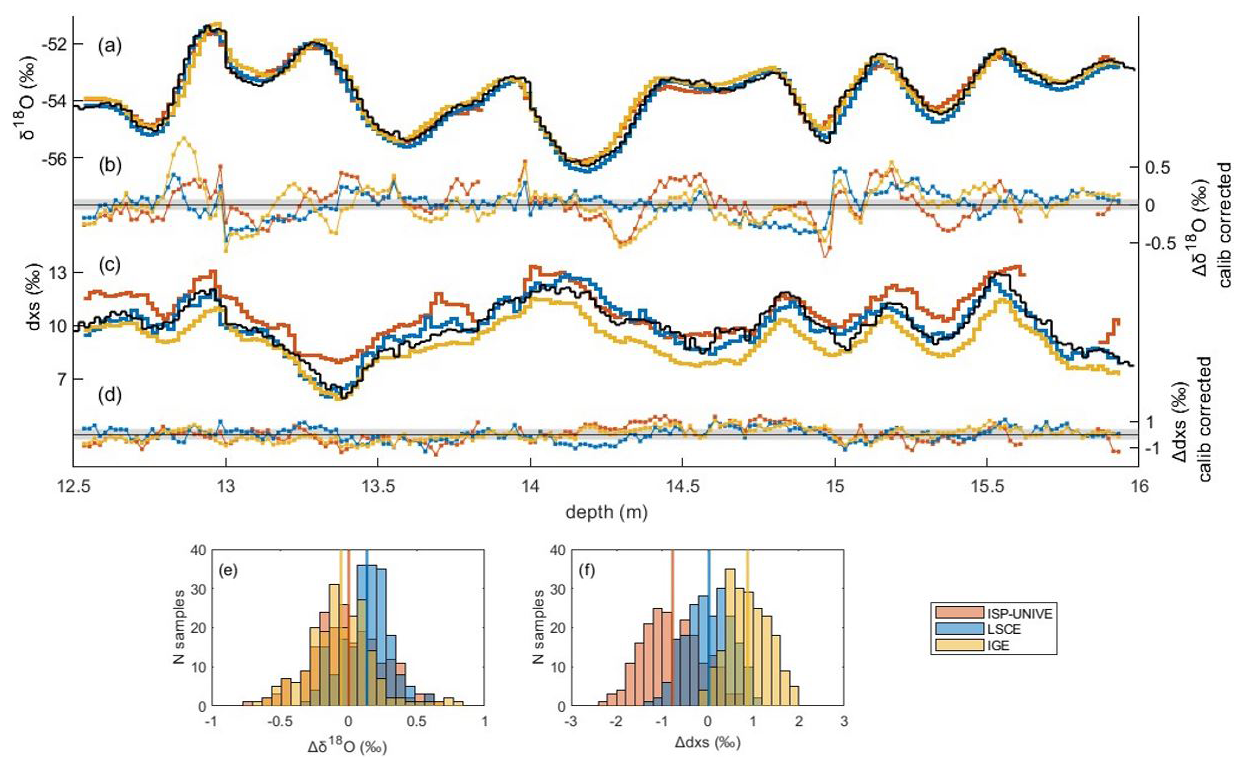
Figure 7 (a, c) Comparison of discrete δ¹⁸O and d-excess profiles (black lines) for the depth interval of 12.5–16 m with integrated discrete records built from CFA measurements for ISP-UNIVE (orange), LSCE (blue), and IGE (yellow). The histograms in (e) and (f) represent the distribution of the difference between discrete data and discrete records built from CFA measurements. Panels (b) and (d) show the difference between discrete data and discrete records built from CFA measurements corrected for calibration. The horizontal grey areas represent the uncertainties of the discrete analysis for δ¹⁸O and d excess.

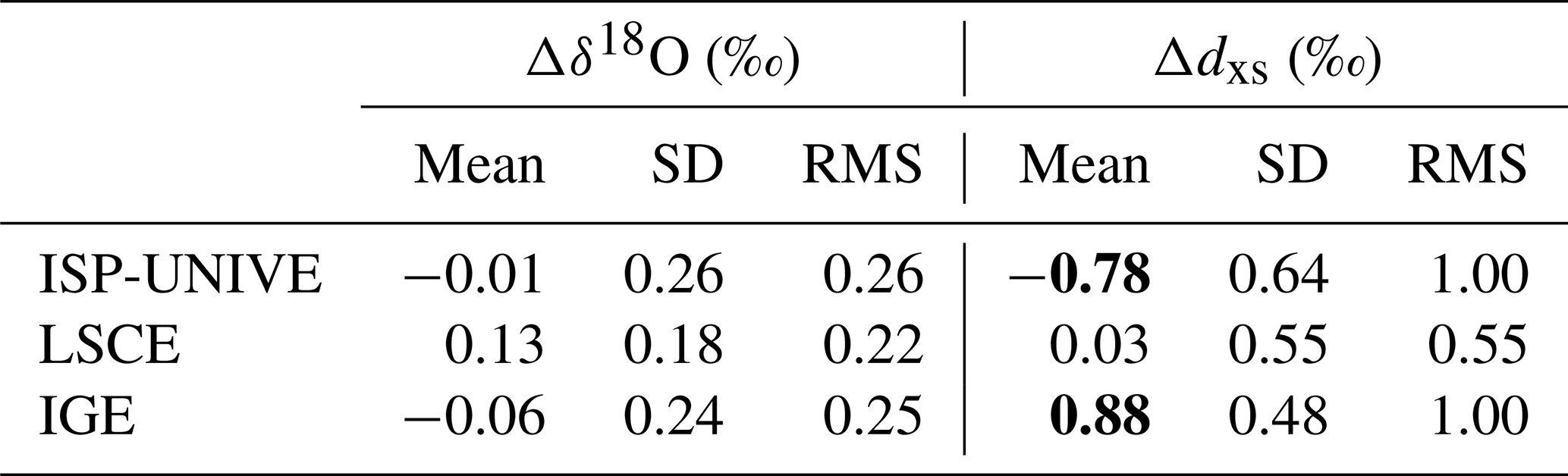
A representative example regarding the x-axis values (melt rates and their associated standard deviation) prior to the conversion into depth is provided in Fig. E1 in Appendix E. The differences between the averaged continuous and discrete data are analysed using histograms of the differences at each depth point (Fig. 7e and f), and statistical significance is assessed using a Kruskal–Wallis non-parametric ANOVA test (Kruskal and Wallis, 1952). Differences with p < 0.05 are considered to be statistically significant. Overall, the variability in ice core δ¹⁸O records, primarily at the decimetric scale, is comparable between the three CFA profiles and the discrete sampling, showing no statistical difference. In detail, the ISP-UNIVE-CFA shows a difference of −0.01 ± 0.26 ‰ (mean ± 1σ). Two data intervals, corresponding to depths of 13.85–13.96 and 15.62–15.85 m, are removed due to the drops in humidity at 1200 and 7850 ppmv following the post-processing procedure described in Sect. 2.5. For the LSCE-CFA, the mean difference for δ¹⁸O is slightly higher but remains non-significant, with an SD within the instrument's error (0.13 ± 0.18 ‰ for δ¹⁸O, Table 5). The IGE-CFA results show a difference of −0.06 ± 0.24 ‰ compared to the discrete data. The SD, similar to that of ISP-UNIVE but larger than that of LSCE, is primarily attributed to small depth scale shifts (Fig. 7b). For d excess, the ISP-UNIVE and IGE show statistically significant differences from the discrete data of −0.78 ± 0.64 ‰ and 0.88 ± 0.48 ‰, respectively. These discrepancies are mostly attributable to calibration, as shown by the reduced difference after applying a calibration correction that aligns the mean difference to zero (Fig. 7d). In contrast, the LSCE record shows a non-significant difference of 0.03 ± 0.55 ‰.

Table 5 Mean, SD, and root mean square (rms) of the isotope difference between discrete and CFA data for ISP-UNIVE, LSCE, and IGE. Significant differences (p < 0.05 using a Kruskal–Wallis non-parametric ANOVA test) are represented in bold.

Overall, the good agreement between CFA and discrete records for both δ¹⁸O and d excess suggests that the LSCE data processing is the most reliable among the three CFA setups, which is why the entire PALEO2 core was analysed at LSCE (Sect. 4).

3.5 Impact of diffusion and mixing on the signal

In this section, we conduct a PSD analysis on continuous and discrete results (Fig. 8) to assess the impact of mixing on continuous measurements and to determine the frequency limit at which the measurement noise begins to dominate over the signal. The continuous data have a post-processed resolution of 0.5 cm, while the discrete samples have a resolution of 1.7 cm. Diffusion, with a length of 6–8 cm in firn, begins to smooth the climatic signal at periods around 50 cm (as observed in the yellow areas of Fig. 8). In the range of 20–50 cm (yellow area), diffusion emerges as the dominant process shaping the spectra. At smaller scales (3–20 cm – orange area), however, additional mixing, characterised by mixing lengths of a few centimetres, further attenuates the power preserved in the discrete spectrum. This power is not only associated with instrumental noise but may be attributed to additional post-depositional processes occurring in parallel with or after diffusion, which will not be investigated in this study. The frequency limit for reliable isotopic measurements corresponds to the intersection of the smoothed signal (dashed black lines, S) and the noise flat spectrum (brown areas, dashed black lines, ε_N), where the SNR is equal to 1. These resolution limits are 1.8 cm for ISP-UNIVE, 1.6 cm for LSCE, and 1.3 cm for IGE. While the effects of mixing can be corrected by applying back-diffusion to the signal, attempting this on frequencies dominated by measurement noise would result in an artificial amplification of that noise. However, as the primary objective of this study is to provide a straightforward approach for determining the resolution at which measurement noise begins to dominate the signal, the records will be custom block averaged at that determined resolution. This process effectively removes measurement noise, additionally removing the amplification of noise that could result from back-diffusion process.

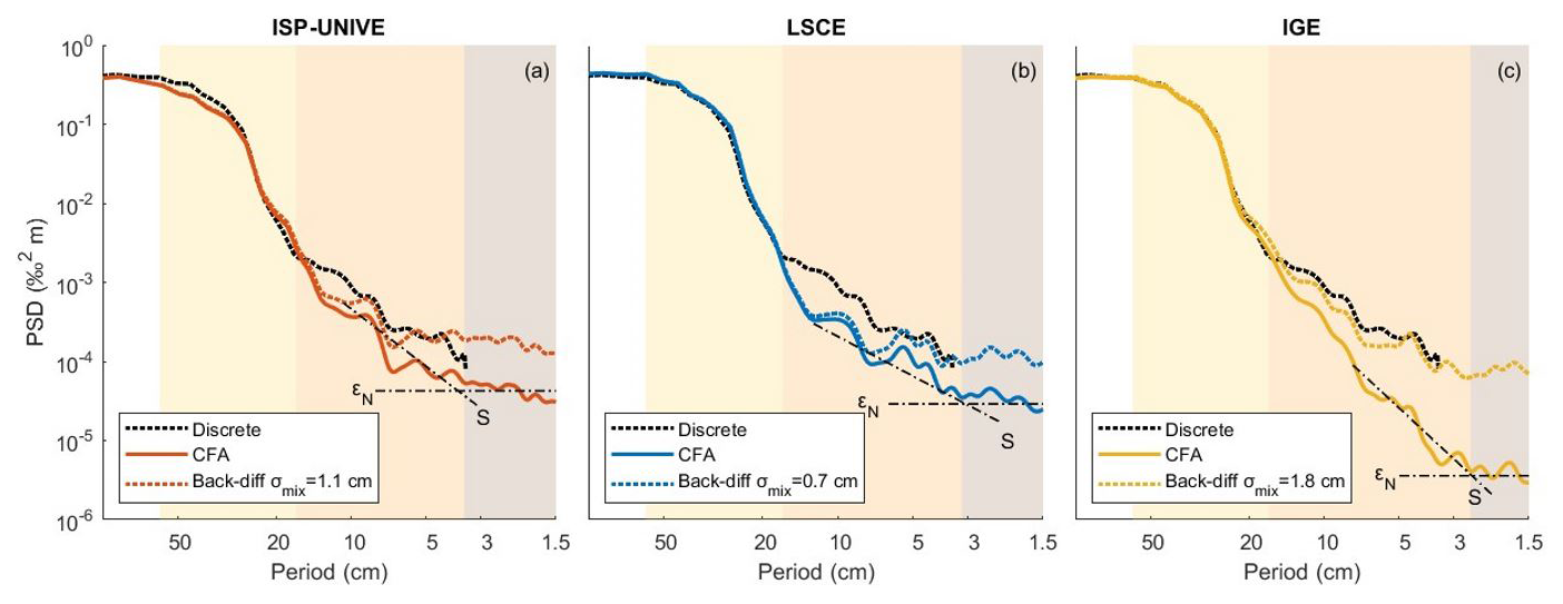
Figure 8 PSD of continuous and back-diffused data compared to discrete spectrum for (a) ISP-UNIVE, (b) LSCE, and (c) IGE. The crossing point of the dotted lines, representative of the nearly flat white noise (ε_N) and the signal (S), corresponds to SNR = 1. For each system, the shading areas represent the period range at which diffusion in firn (yellow), mixing in the CFA (orange), and measurement noise (brown) dominate.

The filter used for deconvolving the mixing effect in isotopic time series applies a back-diffusion method using a Gaussian kernel-based approach (Wasserman, 2006). Taking the time series and the nominal σ_mix (Sect. 3.3) as input, for each data point in the time series, a Gaussian kernel is constructed based on the mixing length. The kernel is centred on the current point and is extended to the surrounding points, with the width of the kernel being determined by the diffusion length. The kernel is then normalised, and the values within the kernel range are weighted and convolved with the original data to produce a diffused value for each point. This smoothing process captures the effects of diffusion, generating an artificial diffused record. Then, the inverse Fourier transform is calculated based on the difference between original and diffused signals and is applied to the original signal to restore the higher frequencies. The back-diffused profiles show significant improvement in the amount of signal across the 3–10 cm period range for all three CFA systems. The lack of signal for periods ranging from 10 to 20 cm in the LSCE profile and, to some extent, in the ISP-UNIVE is not corrected by this back-diffusion, which does not act at such frequencies. However, although we observe a correction of the high frequencies in the spectral domain, this adjustment proves to be negligible when comparing the back-diffused data with discrete samples along the depth scale (Fig. F1 in Appendix F). This is because the signal is dominated by low frequencies – with approximately 1000 times more power at the 50 cm scale than at the 10 cm scale – and because the restored high-frequency power remains relatively weak.

4 Discussion

The comparison of isotopic continuous and discrete records from the 4 m PALEO2 firn core highlights the advantages and limitations of the operating procedures and technical features of three CFA-CRDS systems developed at ISP-UNIVE, LSCE, and IGE (Table 6). Regarding its time efficiency, using the LSCE-CFA system, we were able to analyse the 18 m PALEO2 firn core in 2 d (Fig. 9). The cutting of the sticks was done in parallel to the melting, avoiding the storage of the firn for extended periods of time and allowing for immediate resampling if needed. In contrast, discrete processing and analysis at 1.5 cm of the 4 m core section took over a month. Extrapolating this analytical payload, analysing the entire PALEO2 core would take more than 5 months. A notable limitation of the CFA setup is its application to the low-density upper part of the cores (specifically, the upper 2 m for the PALEO2 core), where challenges in controlling melting speed and stick collapse require the use of discrete measurements rather than CFA. As previously found at the other institutes equipped with a CFA, the precisions for discrete and continuous flow analyses are equivalent (Gkinis et al., 2011; Emanuelsson et al., 2015; Jones et al., 2017a). Here, by using PSD to evaluate the effective resolution imposed by measurement noise in addition to the precision, we were able to determine the resolution at which records can be interpreted: 1.8, 1.6, and 1.3 cm for ISP-UNIVE, LSCE, and IGE, respectively. The primary factors affecting the precision and the resolution are the performance of the Picarro instrument and the humidity level maintained during the analysis. Indeed, by setting the effective resolution at which the impact of mixing can be removed from the signal, using an instrument with better precision will directly improve the signal. For instance, implementing a VCOF-CRDS instrument with 20-fold better precision (Casado et al., 2024) could reach millimetric effective resolution.

Table 6 Summary of the main advantages and limitations identified in the CFA-CRDS comparison.

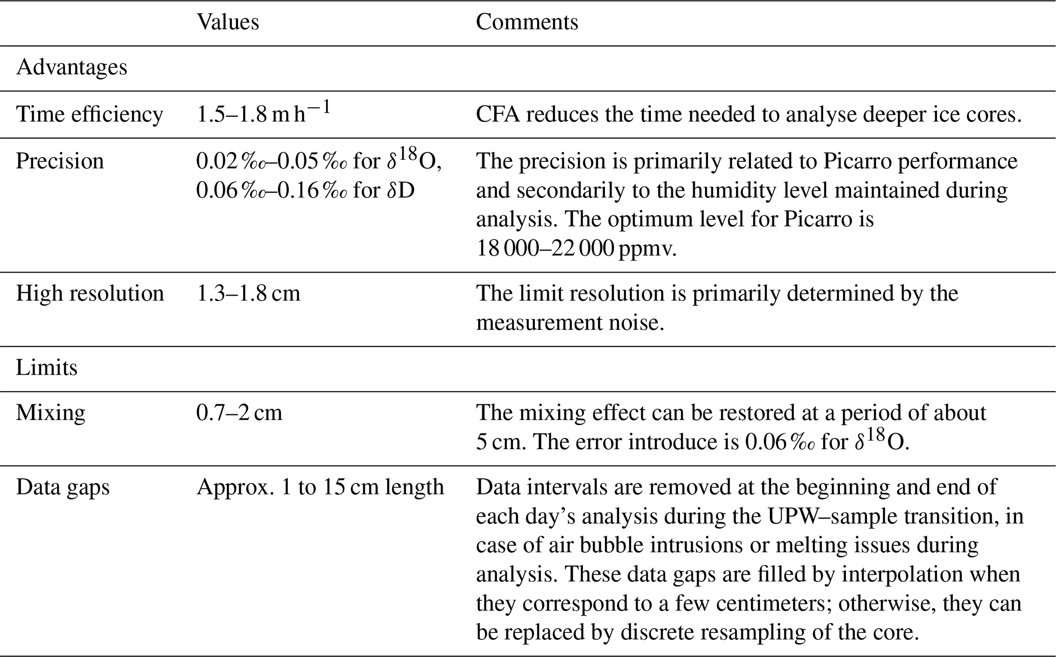
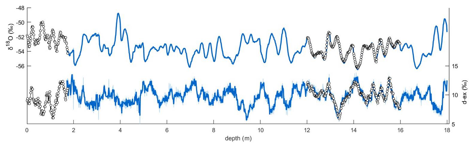
Figure 9 The 18 m PALEO2 core analysed with the CFA-CRDS system at LSCE. The δ¹⁸O and d-excess profiles of the raw data (light blue), block-averaged at 1.6 cm data (blue), are shown with the discrete results (white dots).

Maintaining a constant high humidity level is crucial for mitigating performance variations (Davidge et al., 2022) as this was identified as the key factor responsible for the difference between the ISP-UNIVE-CFA and discrete results. The impact of humidity level on the measurements is around 0.015 ‰ per 1000 ppmv for δ¹⁸O and 0.216 ‰ per 1000 ppmv for δD. Although these values are well within the uncertainty of the Picarro instrument, it is crucial to keep the humidity variation within a maximum range of 6000 ppmv during daily CFA analyses to ensure that this effect remains negligible.

Additionally, the CFA method is limited by mixing within the system, which smoothes the measured signal. In this study, we focused on and presented results relative to firn cores. However, the impact of diffusivity may differ in deeper and denser sections of the ice core due to variations in ice porosity. Furthermore, changes in melt-head temperature and melt rate settings for denser core analyses may also influence the mixing impact. Therefore, additional tests are needed to accurately characterise mixing in deeper ice. We validated the mixing lengths evaluated by means of a step function through PSD analysis of the back-diffused profile for each of the three systems, confirming that the σ_mix derived from ice-to-firn, firn-to-ice, and ice-to-ice transitions serves as a reliable surrogate for the realistic case of firn-to-firn transitions. Furthermore, although our study focused on low-density firn cores, we expect these findings to remain valid – or potentially improve – for deeper core sections, given the reduced mixing that is likely to occur at the melt-head stage. The IGE-CFA system, characterised by a longer distribution line, a 1000 µL volume debubbler, and two dust filters, results in the longer σ_MH (1.8 ± 0.3 cm). However, this increased mixing length is compensated for by the low noise level of the high-performance analyser, which enhances the effective resolution.

Back-diffusion can effectively mitigate the mixing effect at high frequencies. However, while the corrected data show a ∼ 0.1 ‰ gain in isotopic signal in the proximity of the climatic peaks, the improvement compared to the discrete profile is very limited. This is consistent with the PSD of both continuous and discrete records, where the signal is dominated by longer periods (20–100 cm, with a power of 10⁻¹ ‰² m–10⁰ ‰² m); while, at the mixing scale (10–20 cm), it is associated with lower power (10⁻³ ‰² m–10⁻⁴ ‰² m) comparable to the instrumental limit. These findings suggest that the impact of back-diffusion correction is limited for cores recording inter-annual to decadal signals (Münch and Laepple, 2018; Casado et al., 2020). However, this may become crucial in records with greater variability at shorter depth scales, such as for deeper core sections where decadal signals are compressed into smaller depths. It is also relevant when analysing significant events, like those associated with atmospheric rivers (Wille et al., 2022), in areas where firn diffusion does not significantly erase the signal, unlike at the PALEO site. Furthermore, removing the effects of firn diffusion occurring prior to ice core drilling will require the application of a back-diffusion function, along with accurate estimates of variability on centimetric scales (Jones et al., 2017b).

The LSCE-CFA, characterised by the lower discrepancy compared to discrete results (Fig. 7e and f), has a maximum potential resolution of 0.7 cm according to the mixing length. However, the actual achievable resolution for this specific measurement campaign is limited to 1.6 cm due to the relatively low performance of the vaporiser Picarro system. This suggests that using a better Picarro analyser, characterised by a better Allan variance, could significantly improve the LSCE-CFA setup's performance. Here, we argue that the signal measured with the LSCE-CFA from the PALEO2 firn core (Fig. 9) accurately reflects the isotopic variability present in the firn in terms of both δ¹⁸O and d excess. Furthermore, the results obtained can be confidently compared to cores measured at the other institutes.

An additional limitation of CFA systems is data loss at the beginning and end of the analysis due to the memory effect of the CRDS analyser. We strongly recommend using an ice stick with an isotopic composition similar to that of the samples before and after the analysis rather than mock UPW ice, as recently suggested by Davidge et al. (2022). For firn analysis, filling the tubes with depleted water of similar isotopic composition to that of the core helps mitigate transitions at the MH during the switch from ice to firn. Since memory effects decay exponentially, the length of data that must be removed to eliminate this effect depends on the isotopic composition difference. At IGE, a mock UPW ice with δ¹⁸O composition of −12 ‰ precedes ice core analyses. For a δ¹⁸O difference of about 40 ‰ between mock and sample ice, approximately 9.5 cm of the record must be removed. Conversely, for an ice stick with a δ¹⁸O difference of 3 ‰–4 ‰, only the first 1.8 cm is affected by the memory effect.

To ensure reliable isotopic records, we list recommendations for future improvement or setting up of a CFA-CRDS system:

• First, developing a short transport line and then selecting a low-volume debubbler can reduce mixing.

• Installing conductivity devices both downstream of the MH and upstream of the CRDS instrument ensures accurate depth scale attribution.

• Using ice sticks or filling the tubes with water of similar isotopic composition to the samples rather than UPW ice helps reduce memory effects. In addition, avoiding the use of UPW water in the system during the analysis to clean the line minimises data loss (Dallmayr et al., 2025).

• Conduct pre-analysis testing of the core density to determine the appropriate MH temperature for achieving the desired flow rate and select a melting rate that allows for a long integration time to enhance measurement precision.

• Maintaining constant high humidity levels for isotope analysis (optimal range for the Picarro instrument: 18 000–22 000 ppmv) mitigates performance variations (Gkinis et al., 2010; Davidge et al., 2022).

5 Conclusions

The technical intercomparison of the three CFA-CRDS systems developed at ISP-UNIVE, LSCE, and IGE highlighted each system's strengths and identified opportunities for future optimisation and development. Operating at a melt rate of 2.5–3 cm min⁻¹ under stable conditions, these systems measure 8–10 m of firn core per day, confirming that CFA-CRDS is a fast, high-resolution method for isotope analysis, with precision comparable to the discrete method. For ISP-UNIVE-CFA and LSCE-CFA systems, the main limitation in achieving a higher resolution is imposed by the performance of the analyser. Conversely, the IGE-CFA system, with the great advantage of providing chemistry measurements online, has a setup limitation related to its longer distribution line and higher volume debubbler, which promotes mixing. To optimise system performance, it is crucial to set a melt rate high enough to ensure sufficient flow for all instruments and fraction collectors in the CFA system while minimising excessive mixing at the melt head and in the tubing and without extending the duration of the CFA campaign for melting the core.

Finally, the outcomes of this work provided the basis for the analysis of four PALEO cores analysed at ISP-UNIVE, LSCE, and IGE as part of the EAIIST project (Traversa et al., 2023), enabling the determination of the maximum reliable resolution achievable with CFA for interpreting the climatic signal in ice cores.

Appendix A: Allan variance for different humidity levels ranging from 10 000 to 20 000 ppmv

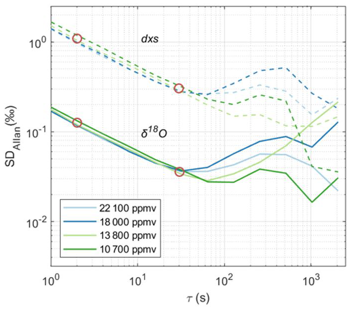
Figure A1 δ¹⁸O and d-excess Allan variance computed from 1 h continuous UPW flow for humidity levels ranging from 10 000 to 20 000 ppmv. Red circles indicate integration times (τ) equal to 2 and 30 s, needed to melt 0.1 and 1.5 cm, respectively.

Table A1 Allan variance for δ¹⁸O, δD, and d excess with respect to the integration times (τ) needed to melt 0.1 and 1.5 cm of the ice core at a melting rate of 3 cm min⁻¹.

Appendix B: Continuous measurement of UPW

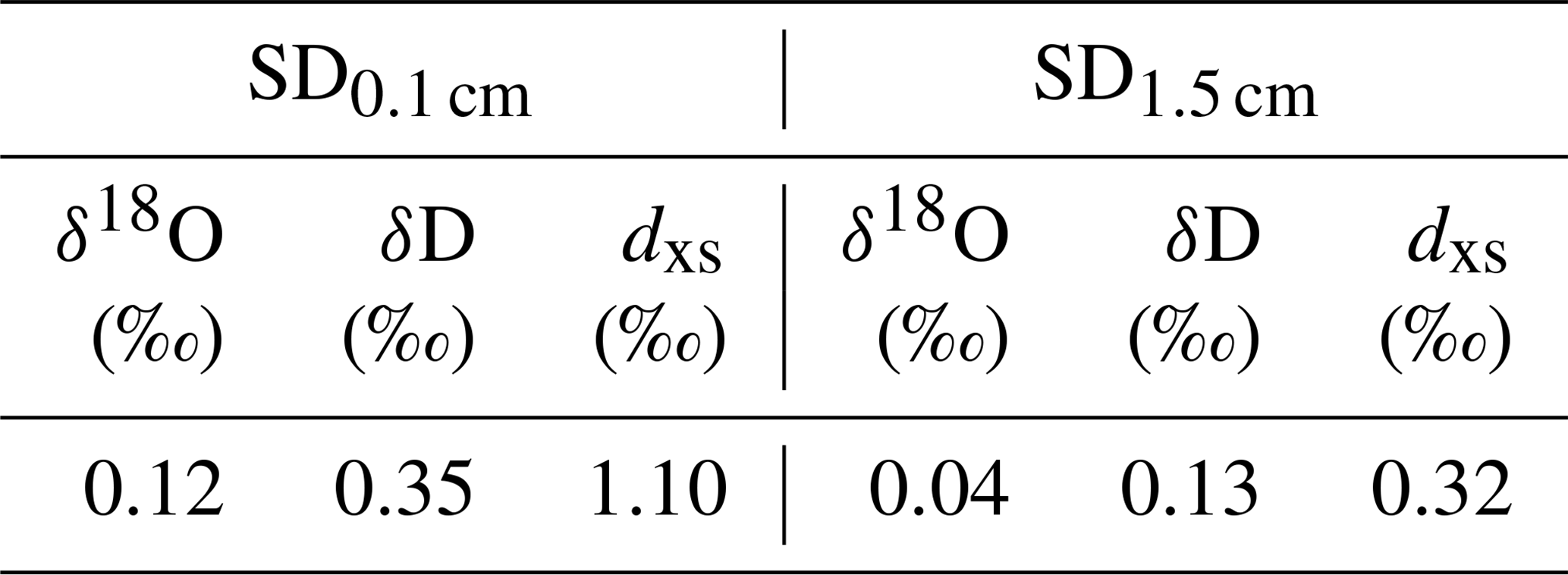
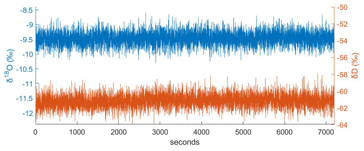
Figure B1 δ¹⁸O and δD results from a 2 h continuous injection of UPW at ISP-UNIVE (∼ 14 000 ppmv).

Appendix C: Mixing lengths evaluated at MH and SV stages

Table C1 δ¹⁸O mean mixing lengths (σ_MH) at the stage of the melt head derived from the normal PDF calculated for N number of firn-to-ice, ice-to-firn, and ice-to-ice isotopic steps. The σ_MH is the mean value of all of the steps for each institute. The lengths are expressed in millimetres, accounting for the nominal melting speed, and the respective 1SD values are in parentheses. The σ_SV is obtained from the steps at the selector valve stage.

Appendix D: CRDS processed data at 0.5 cm in comparison with record constructed at 1.5 cm and discrete data

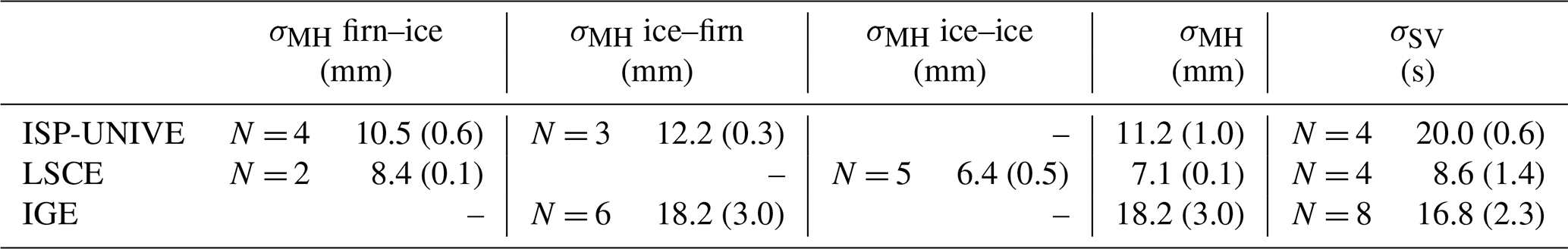
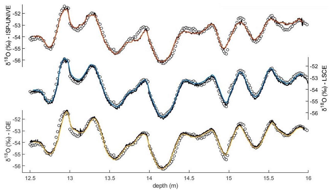
Figure D1 Comparison of δ¹⁸O from CFA post-processed data at 0.5 cm resolution (black lines) and discrete values (white dots). Coloured lines show discrete records constructed from CFA measurements at a 1.5 cm resolution after calibration correction.

Appendix E: The x-axis melt rate values and associated standard deviations

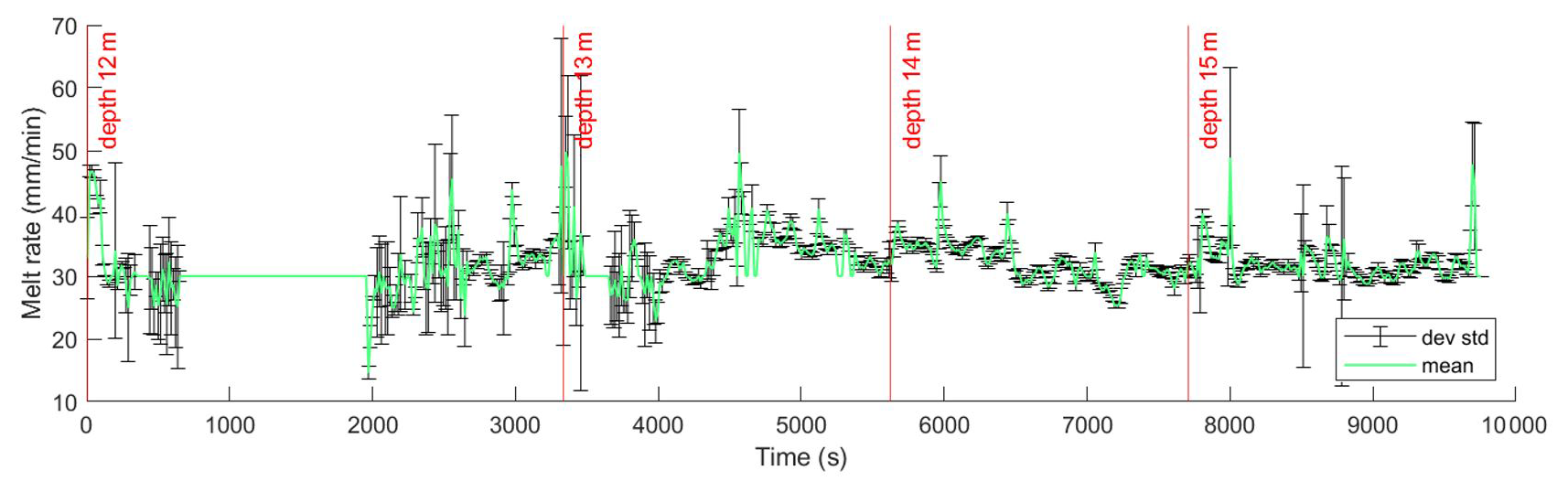
Figure E1 Mean melt rate variations and associated standard deviations computed over ∼ 15 s intervals from the IGE dataset, corresponding to an approximate depth resolution of 0.5 cm.

Appendix F: Sensitivity test of the evaluation of the mixing length

Back-diffusion can mitigate the mixing effect at higher frequencies. To quantify the gain in isotopic composition, we present the continuous δ¹⁸O IGE profile back-diffused with σ_mix = 1.8 ± 0.3 cm (Fig. F1). To prevent amplification of measurement noise, high frequencies with a signal-to-noise ratio (SNR) below 1 are removed by block averaging the profile at the specified frequency limit. Block averaging aggregates isotope records to a new depth scale resolution, defined by each system's frequency limit. The original data are averaged within each interval and assigned to the corresponding depth point on the new scale. When comparing the raw data and the back-diffused profiles, we observe a gain of up to 0.1 ‰ in proximity of the climatic peaks. However, since, through PSD analysis, both continuous and discrete records show very low power at the mixing length scale compared to the power of the dominant signal, it is evident that the back-diffusion approach has a limited impact on restoring the signal when compared to the discrete profile.

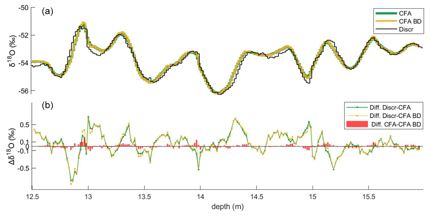
Figure F1 (a) Discrete δ¹⁸O record (black) compared with IGE-CFA profile (green) and back-diffused profile using σ_mix = 1.8 cm (yellow). (b) The difference between the discrete record and the original CFA profile (green) and the back-diffused profile (yellow line). Red bars represent the difference between CFA and back-diffused data.