A new approach to characterizing medium-scale gravity waves using Antarctic airglow observations

Medium-scale gravity waves (MSGWs) are atmospheric waves with horizontal scales ranging from 50 to 1000 km that can be observed through airglow all-sky images. This research introduces a novel algorithm that automatically identifies MSGWs using the keogram technique to study the waves over the Antarctic Peninsula. MSGWs were observed with an all-sky airglow imager located at the Brazilian Comandante Ferraz Antarctic Station (CF, 62° S), near the tip of the Antarctic Peninsula. Several preprocessing techniques are necessary to extract the parameters of MSGWs from the airglow images. These include projecting the images into geographical coordinates, applying a flat-field correction, performing consecutive image subtraction, and employing a Butterworth filter to enhance the visibility of the MSGWs. Additionally, a wavelet transform is used to identify the primary oscillations of the MSGWs in the keograms. Subsequently, a wavelet transform is also used to reconstruct the MSGWs and obtain the fitting coefficients of phase lines. The fitting coefficients are then used to calculate the MSGW parameters and assess the quality of the results. Simulations with synthetic images containing typical propagating gravity waves were conducted to evaluate the errors generated during the MSGW calculations and to determine the threshold for the fitting parameters. This methodology processed a year's worth of data in less than 1 h, successfully identifying most waves with errors lower than 5 %. The observed wave parameters are generally consistent with expected results; however, they show differences from other observation sites, exhibiting larger phase speeds and wavelengths.

1 Introduction

Atmospheric gravity waves are an essential feature of atmospheric motions due to their energy and momentum driving across the atmospheric layers (Nappo, 2002; Fritts and Alexander, 2003). Gravity waves over the Antarctic region transport momentum and energy through the atmosphere (Plougonven et al., 2013; Moffat-Griffin et al., 2011; Lu et al., 2015), playing a major role alongside other phenomena like the stratospheric polar vortex, polar night jet (PNJ), and mesospheric polar clouds (Moffat‐Griffin and Colwell, 2017; Zhao et al., 2015). They can also transport energy from one region to another due to their horizontal movement, influencing the dynamic features of the entire planet (Kogure et al., 2018; Vadas et al., 2019).

To understand gravity waves' influence in the atmosphere, previous studies have measured gravity wave characteristics to parameterize their effects depending on their observed scales (Vosper et al., 2018; Lehner and Rotach, 2018). To achieve this, observations must include large datasets and account for both short- and long-term variations in the characteristics of waves to associate them with environmental features and behaviors (Song et al., 2021).

Instrumental biases are crucial to consider when observing gravity waves. The resolution of an instrument determines the dimensions of the waves it can detect, which is called the observational filter: an instrument with a poor temporal (spatial) resolution cannot detect waves with a period (wavelength) of less than twice its resolution, as stated by the Nyquist theorem. Thus, reliable estimation of the wave period (wavelength) requires a higher sampling resolution (Wright et al., 2016, 2017). Temporal and local continuity are also significant factors in studying propagating waves, as waves can be intermittent or fast enough not to be detected if the observations are not continuous (Plougonven et al., 2017; Alexander and Barnet, 2007). For instance, while satellites can provide global coverage and track seasonal variations, they often miss local features and properties associated with wave movement because they do not observe a single location continuously (Ern et al., 2004; Alexander et al., 2015). However, a ground-based instrument can miss the wave movement if it has a large structure and propagates beyond the observing region (Beldon and Mitchell, 2009; Wu et al., 2013). Moreover, the computational methods applied to the data can restrict the observed spectrum (Wright et al., 2021); for illustration, averaging tends to reduce wave information within a dataset, as it cuts the wave modes of the period shorter than the average window.

Airglow imaging is one of the most employed and valuable techniques for observing gravity waves (Swenson and Mende, 1994). Airglow is the atmospheric emission emitted by some constituents excited by photochemical reactions. Many works have used airglow to study gravity waves in the mesopause region, explore their general characteristics and parameters throughout the seasons (Nakamura et al., 1999; Essien et al., 2018), and investigate their general dynamics related to the background conditions (Medeiros et al., 2003; Giongo et al., 2018). To obtain gravity wave parameters and characteristics, most works have employed spectral analysis based on Fourier transforms applied directly on the image to determine the wave parameters (Garcia et al., 1997; Giongo et al., 2020). An airglow camera is relatively low-cost and works for extended periods; aside from its limitation to nighttime observations, it can provide information on (1) small-scale waves and (2) long-term features of the mesopause region by applying the keogram technique to the observations (Taylor et al., 2007).

Numerous observations of small-scale gravity waves in airglow images have been recorded in certain equatorial and tropical regions. The keogram technique has facilitated the study of medium-scale gravity waves at these sites, broadening the observed spectrum and linking these waves to other phenomena, such as plasma bubbles. (Paulino et al., 2011; Figueiredo et al., 2018; Taylor et al., 2009; Bilibio, 2017; Essien et al., 2018; Takahashi et al., 2020).

Observations of medium-scale gravity waves over the Antarctic continent by airglow have not been reported. Additionally, satellite observations may capture waves of similar spatial dimensions, mainly in the stratosphere (Hoffmann et al., 2013; Hindley et al., 2019). Observations using a limb-viewing technique (Alexander et al., 2009; Hindley et al., 2015) are also limited to large horizontal scales. Airglow observations have the advantage of high temporal resolution at a fixed location, allowing the identification of faster and slower waves (Bageston et al., 2009; Nielsen et al., 2009; Kam et al., 2017). By extending the analysis of the airglow data to medium-scale gravity waves, one can determine the phase speed spectra of these waves, similar to the approach taken by Matsuda et al. (2017) for small-scale gravity waves, and relate this spectrum to the background wind filtering or other atmospheric conditions (Perwitasari et al., 2018; Kam et al., 2021).

This study employed the keogram technique to investigate medium-scale gravity waves observed through airglow imaging over the Antarctic Peninsula. The primary objective of this paper is to present a reliable analysis method for these waves, allowing future comparisons at other observation sites and ensuring comprehensive observations of the entire wave spectrum concerning different instruments and techniques. Section 2 describes the data used and introduces a new methodology for analyzing medium-scale gravity waves in keograms. It includes wavelet amplitude correction and the identification of phase fitting quality along the columns of simulated keograms. Section 3 presents the application of the methodology using real keograms of observed images. Section 4 is a study of the errors of the procedure, and Sect. 5 shows the results on observed data, while Sect. 6 drives the discussions on the results and comparison with previous methods. Section 7 presents the main conclusions.

2 Methodology

2.1 Image processing

The data utilized were ground-based airglow images obtained by an all-sky imager installed at the Brazilian Antarctic Comandante Ferraz Station (CF) on King George Island, 200 km from the tip of the Antarctic Peninsula. The imager has a filter wheel for the observations of OH-NIR (700–900 nm), OI 557.7 nm, and 630.0 nm emissions. The camera is cooled to −70 °C and has 80 % quantum efficiency for visible and near-infrared wavelengths (KEO SCIENTIFIC LTD, 2022).

To calculate the medium-scale gravity wave parameters, the following preprocessing procedures were applied to the images: (a) projection of the images into geographic coordinates, (b) removal of stars, (c) application of a flat-field correction, (d) subtraction of images, (e) construction of keograms, and (f) application of a Butterworth filter to reduce noise and eliminate long-term oscillations caused by twilight and moonlight. Each procedure is described in detail below.

The image projection into geographic coordinates used in this work follows the well-established and widely used procedures initially developed by Garcia et al. (1997) and recently improved by Wrasse et al. (2007) with other minor improvements by Bageston et al. (2009) and Giongo et al. (2020). The image projection involves aligning the images with north at the top (east to the right) and projecting them into geographical coordinates on a 1 × 1 km grid, creating 512 × 512 km images of the airglow layer centered over the observation site. The star removal is based on a statistical inference of the neighborhood of the peaks to remove them without interfering with the amplitude of the oscillations in the background. The van Rhijn and atmospheric extinction effects are corrected along with flat-fielding to avoid brightness variations due to the observation angle of the all-sky lens fitted to the camera (Kubota et al., 2001; Wrasse et al., 2024). Additionally, consecutive images are subtracted in order to suppress the Milky Way and other slow-varying features in the images (Tang et al., 2005; Vargas et al., 2021).

Figure 1 shows an example of the original image acquired by the all-sky imager and the resulting preprocessed images following the procedures described above. Figure 1a displays the original image, Fig. 1b shows the star-removed image, Fig. 1c depicts the van Rhijn and atmospheric-extinction-corrected image, and Fig. 1d illustrates the projected image onto a 512 × 512 km grid. Observational distortions due to the lens were successfully removed. The Milky Way is an inconvenient feature in the images that will not be a problem for the analysis, as discussed later.

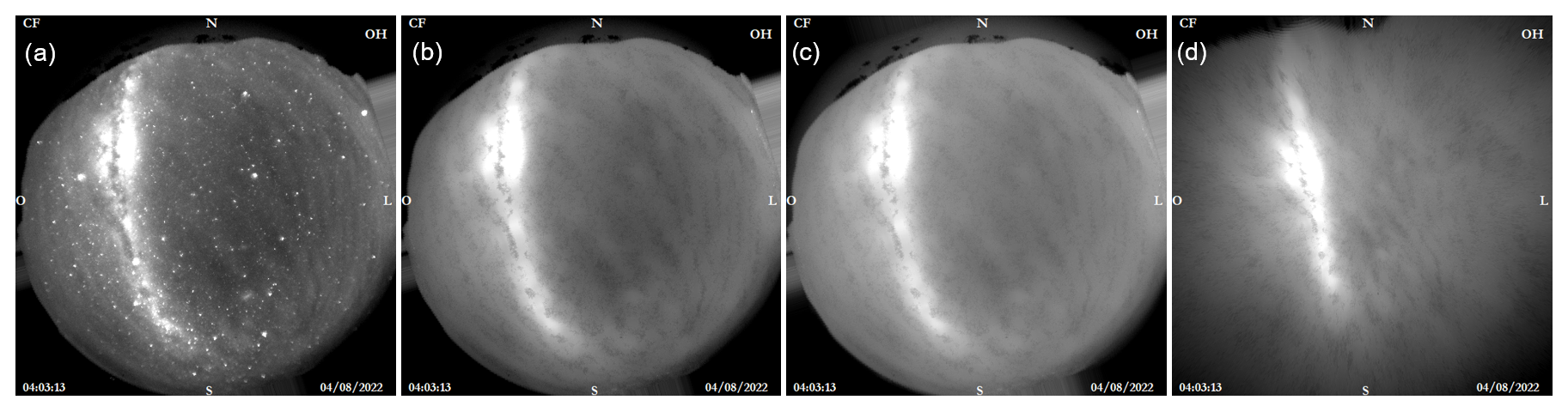
Figure 1 A series of images demonstrating the preprocessing steps applied to an airglow image.

Keograms are formed by choosing a sample from the central row and column of each image taken during a single night and then stacking them over time. This process produces a diagram that reveals long-period oscillations along with zonal and meridional components. (Taylor et al., 2009; Figueiredo et al., 2018). A Butterworth filter is applied to each time series (lines of the keogram) with cutoff periods of less than 20 min and greater than 240 min to highlight the possible wave periods observable in the images. These limits were chosen based on prior understanding of the technique's constraints: shorter periods corresponding to high-frequency waves can be easily analyzed using alternative methods; in comparison, longer periods (greater than 4 h) may surpass the observation duration and are, thus, excluded from the analysis. Additional information about the typical observation length and the cone of influence (COI) will be discussed later.

Figure 2 presents (a) an example of a keogram and (b) its post-processed form following the aforementioned procedure. In both keograms, the upper panel depicts a zonal component of the keogram created from horizontal slices of the images, while the lower panel illustrates a meridional component composed of vertical slices. The time axis represents the maximum observation duration of the night at CF, with the blank area caused by the limited observation time on this specific night. As the airglow images are measured in arbitrary units (which also depend on exposure time), the scale is simply adjusted between the bright interval's maximum and minimum. Despite the change in scale, the desired oscillations are now more clearly observable.

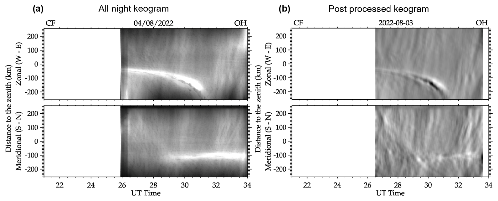
Figure 2 Panel (a) presents an example keogram. Panel (b) is similar to panel (a) but it incorporates all of the mentioned preprocessing steps. At the top, the zonal keogram utilizes west–east samples from the images, whereas the bottom features north–south samples. Both examples are in grayscale, within their maximum and minimum values.

2.2 Spectral analysis

In this work, we develop a new method for analyzing medium-scale gravity waves (MSGWs) based on a wavelet transform described by Torrence and Compo (1998) to calculate the gravity wave parameters. Although the procedure is based on the Fourier transform as in previous works, the distinctive feature of this methodology is that it automatically selects the waves along the keogram and evaluates the quality of the oscillatory signal concerning the wavelet phase properties, resulting in outcomes with reduced reliance on users' judgment. In the following section, we outline the algorithm used for spectral analysis, including the temporal and spatial selection of waves on the keogram. We then demonstrate the procedure using synthetic simulated images that feature propagating gravity waves. The subsequent section illustrates the application of the method using observed airglow images to create the keograms. Finally, Sect. 4 presents a study on error estimation related to this procedure.

2.2.1 Overview and concepts

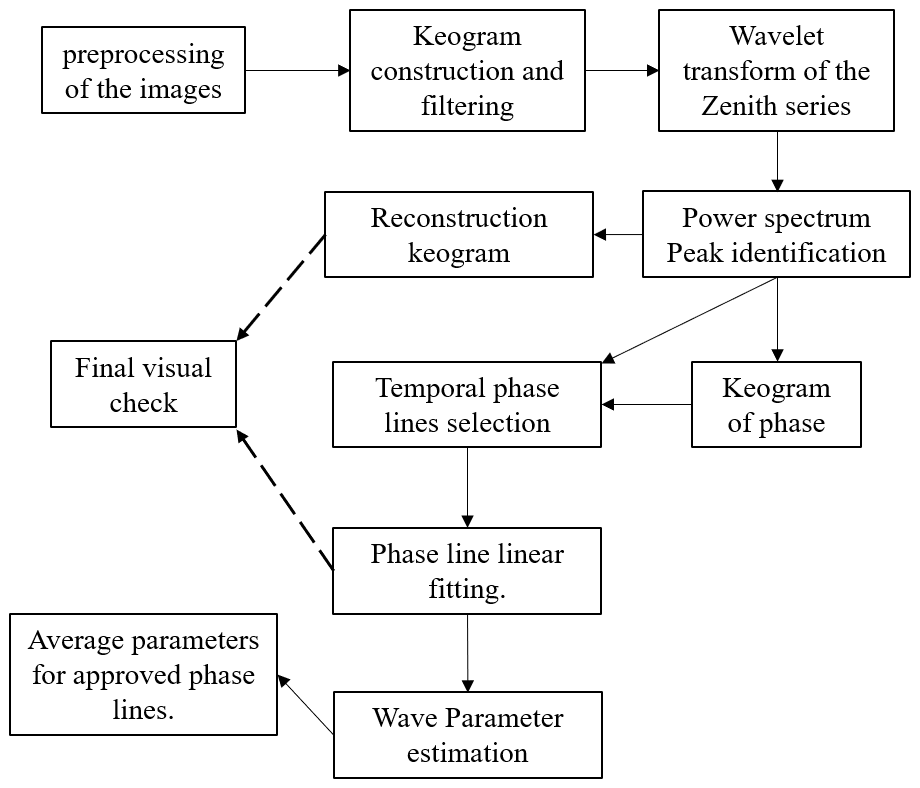
The analysis methodology is summarized in the flowchart in Fig. 3, along with detailed descriptions of each step in the procedure below. Following the preprocessing of images and the creation of the keogram, a Morlet wavelet transform is carried out on the zenith time series. The MSGW parameters are obtained using the reconstruction and phase keograms derived from the wavelet.

Figure 3 Flowchart of the analysis procedure.

When applying a wavelet transform to a time series S(t), we obtain a complex function that depends on time and period: W(t,τ). The power spectrum, defined as the squared amplitude of the wavelet, $\left|W\right(t,\mathit{\tau }){|}^{\mathrm{2}}$ is used to determine the amplitude of the current waves and their position in time and period by locating their peaks on the spectrum. In addition to the amplitude spectrum, we have the phase spectrum, usually defined as follows (Torrence and Compo, 1998):

$$\mathrm{\Psi }(t,\mathit{\tau })=T{g}^{-\mathrm{1}}\left({\displaystyle \frac{\mathit{Im}\left[W(t,\mathit{\tau })\right]}{\mathit{Re}\left[W(t,\mathit{\tau })\right]}}\right),$$

where Im and Re are the imaginary and real parts of the function, respectively; for a fast Fourier transform (FFT), this phase spectrum can be identified as the phase lag of a cosine function fitted to the series with a period equivalent to that used in the fitting. For example, if we fit a function on the general form f(t) = Acos (ωt+ϕ), the phase lag, ϕ, is identified as the phase spectrum of the FFT, for the period equivalent to ω = $\frac{\mathrm{2}\mathit{\pi }}{\mathit{\tau }}$. For the wavelet, we interpret the phase spectrum as the phase position at that time for a fitted cosine with the period τ; that is, the wavelet also gives us information about the phase spectrum over time.

The keogram is then reconstructed by analyzing all of the time series using the period selected in the power spectrum, thereby applying the keogram to the period of interest. This approach is useful for verifying whether the wave with the specified period is present in areas beyond the zenith. A phase keogram could also be generated for the chosen period. As the phases along the lines are regular linear functions (due to the wavelet fitting), we decided only to select a vertical phase line. From this point forward, we refer to the phase along the columns of the phase keogram as phase lines.

At this point, we assume that, when reconstructing all the time series independently, the phase position along the vertical of the keogram, which means the phase point of the wave along one image, must vary smoothly to ensure the wave travels smoothly along the images and, consequently, along the columns of the keogram. This assumption is the main point of the methodology. The applied linear fit will check the wave parameters, wave coherence, and temporal presence using wavelet properties. The phase line is selected when the peak period is present in the power spectrum.

The next step involves checking the phase lines of the reconstruction. Phase lines surrounding the temporal identified peak in the power spectrum are used to perform the linear fit. The linear fit of the format y = αx + β is conducted across all sections of the central phase line. The region where the fitting performs best will be used in all selected lines to evaluate the angular coefficient (α) of the fitting applied in estimating the wave parameters. In conclusion, the position of the phase lines used for parameter estimation is automatically selected based on the fitting quality, without human intervention.

The MSGW parameters are then estimated using the angular coefficient of the phase fit. We interpret α as the change of phase, Δψ, of the wave along the space (columns of the keogram). The following equation estimates the wavelength components (Figueiredo et al., 2018):

$$\begin{array}{}\text{(1)}& {\mathit{\lambda }}_{\mathrm{NS},\mathrm{EW}}={\displaystyle \frac{\mathrm{\Delta }d}{\mathrm{\Delta }\mathit{\psi }/\mathrm{360}}},\end{array}$$

where λ_NS,EW represents the wavelength components (EW for the zonal keogram and NS for the meridional one) and Δd is the distance between the lines of the keograms (spatial resolution of the images). The horizontal wavelength λ_H is then calculated using geometry (Nyassor et al., 2025):

$$\begin{array}{}\text{(2)}& {\mathit{\lambda }}_{\mathrm{H}}={\displaystyle \frac{{\mathit{\lambda }}_{\mathrm{NS}}{\mathit{\lambda }}_{\mathrm{EW}}}{\sqrt{{\mathit{\lambda }}_{\mathrm{NS}}^{\mathrm{2}}+{\mathit{\lambda }}_{\mathrm{EW}}^{\mathrm{2}}}}}.\end{array}$$

The period is estimated directly by the peak position of the wavelet transform and is also used to reconstruct the keogram. The phase speed is calculated as a function of the wavelength and the period following the relation

$$\begin{array}{}\text{(3)}& C_{\mathrm{H}}={\displaystyle \frac{{\mathit{\lambda }}_{\mathrm{H}}}{\mathit{\tau }}}.\end{array}$$

The geometry of the wavelength components finally estimates the wave phase propagation direction:

$$\begin{array}{}\text{(4)}& \mathit{\theta }={\cos }^{-\mathrm{1}}\left[{\displaystyle \frac{{\mathit{\lambda }}_{\mathrm{H}}}{{\mathit{\lambda }}_{\mathrm{NS}}}}\right],\end{array}$$

where cos ⁻¹ is the function that retrieves the angle whose cosine is the input.

Finally, the results and performance of the procedure are visually checked and validated through the keogram reconstruction and the quality of phase lines. Assumptions made by the user include flat and parallel phase lines as well as uniform wave behavior along the reconstruction. Section 4 discusses further details about the fitting quality of phase lines and the method's uncertainties.

2.2.2 Applying the methodology to simulated gravity wave images

This section outlines the methodology for calculating the MSGW parameters in synthetic images. The images are generated with specific wave properties, including wavelength, phase propagation direction, and period. Additionally, wave movement can be incorporated into a sequence of images by considering the phase speed and the time difference between images (time resolution).

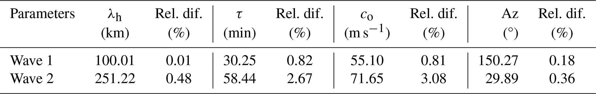
Figure 4 illustrates an example of a keogram generated from synthetic images. Figure 4a presents a synthetic image, while Fig. 4b displays another example, separated by several minutes in time, with the wave fronts highlighted. In this case, two waves are superimposed, with wavelengths of 100 and 250 km, periods of 30 and 60 min, phase speeds of 55 and 69 m s⁻¹, and azimuthal propagation directions of 150 and 30°, respectively. Figure 4c shows the resulting keogram from a set of 200 images with a resolution of 2 min. The waves maintain the same propagation direction in the zonal component, while the opposite direction appears in the meridional component, as clearly indicated in the keogram. Additionally, the combinations of wave amplitudes are evident in both components.

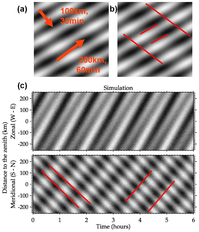
Figure 4 Panel (a) presents an example of a synthetic image with the wave parameters highlighted. Panel (b) is the same as panel (a) but the image is ahead of its time and the phase fronts are highlighted. Panel (c) shows a keogram generated from synthetic images. The grayscale was weighted between the maximum and minimum intervals. Both waves have the same amplitude.

The Morlet wavelet power spectrum applied to the central line of the keograms is shown in Fig. 5, which corresponds to both keograms as it represents the zenith pixel time series. Even with the waves uniformly distributed across all the keograms, the amplitudes decay outside the cone of influence. Although the amplitude of the waves remains consistent, the spectrum is dispersed for the 60 min wave due to the wavelet discretization array. Amplitude corrections are discussed in the next section. Peaks in the wavelet power spectrum are identified using a peak selection procedure to highlight the significant oscillations and their temporal positions. Reconstruction of all time series is conducted for the period determined by the zenith wavelet, resulting in an “enforced” reconstructed keogram for the selected period.

Figure 5 Power spectrum of the simulated keogram.

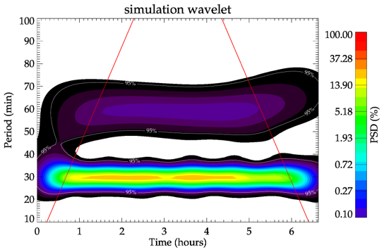
We employed our own method for identifying peaks in the power spectrum, which has been utilized in various published studies related to small-scale gravity waves (Wrasse et al., 2007; Giongo et al., 2020), although none have elaborated on it in detail. The technique consists of identifying the highest value in the power spectrum and excluding an equal number of neighboring points from both sides until a minimum value (half of the peak value) is reached; this process is repeated up to a predefined maximum number of peaks (eight in our case). Despite its simplicity, this method has been effective for detecting peaks in 2D spectra. However, for the wavelet, the number of points in the time domain (x axis) does not match that in the period domain (y axis), which also follows a logarithmically spaced distribution. Our peak selection method operates correctly because we apply linear spline interpolation on a regularly spaced grid, even though the peaks in the power spectrum do not appear uniform along the period axis, which gives them an ellipsoidal shape. Linear spline is a standard regrid method known to prevent amplitude loss. We perform linear spline interpolation on the vertical columns of the spectrum to ensure that the number of points in the vertical matches that of the horizontal lines.

Figure 6 displays the reconstructed keograms and phase lines for the two waves in the simulated keogram, with their periods identified in the power spectrum. Figure 6a and b present the reconstructed keograms for both identified peaks in the simulation power spectrum, while Fig. c and d illustrate the phase lines corresponding to the timings of the peaks in the power spectrum. In the simulation, the peak in power remains consistently present over time, rendering the temporal selection irrelevant; however, we retained the selection methodology. The phase lines were unwrapped to enhance the visualization of the tilt along the columns and to prevent misfitting due to cycle ambiguity. The red sectors emphasize the areas used for fitting.

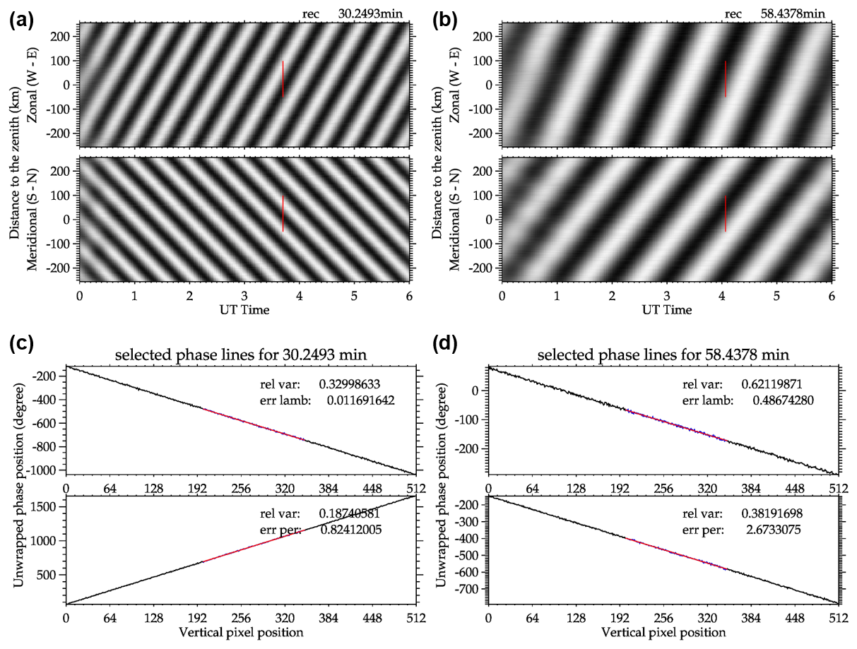
Figure 6 Reconstruction and selected phase lines for the waves in the simulated keogram. (a–b) Reconstruction for the 30 and 60 min waves. (c–d) Phase lines for the 30 and 60 min waves.

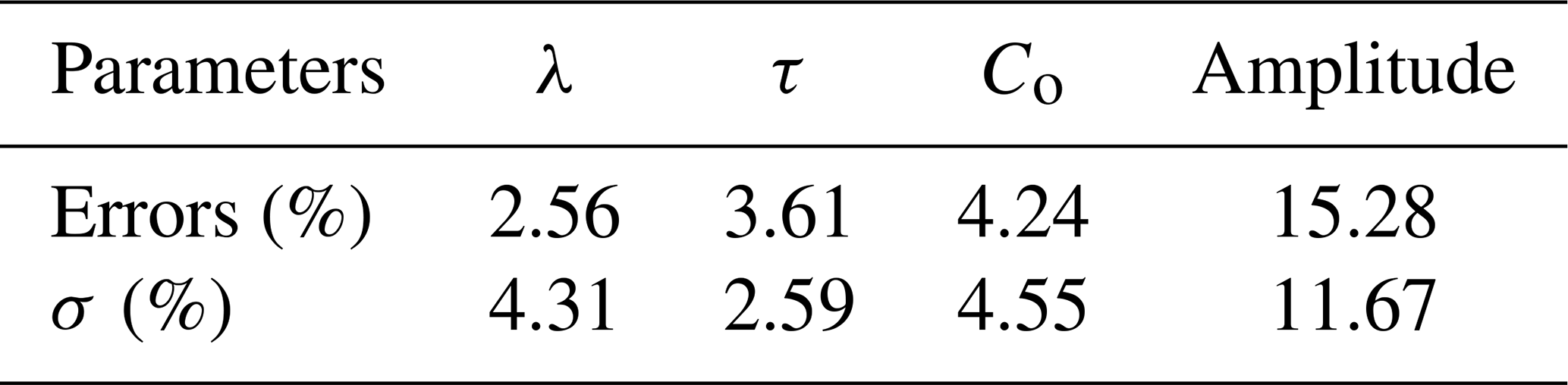
A linear fit is applied to the phase lines, where the angular coefficient is used to calculate the MSGW parameters, as it contains the information on angular differences. At the same time, the fitting provides data for the assessment of the signal quality for the chosen reconstructed period, as demonstrated in Sect. 3. The final results are summarized in Table 1. All results differ by less than 5 % from the simulated gravity wave, showing the consistency of the new methodology. Section 4 discusses further investigation of the differences in the gravity wave parameters throughout the procedure.

Table 1 MSGW parameters obtained by the new methodology, using simulated images of gravity waves. The relative difference (Rel. dif.) values between the simulated and calculated wave parameters are also presented.

2.3 Amplitude corrections

The wavelet transform can directly estimate the amplitudes of the waves, although it requires corrections due to the filters applied to the data and wavelet bias, as reported previously (Torrence and Compo, 1998; Liu et al., 2007). To correct the wavelet biases, we followed the correction proposed by Xu et al. (2024) (and references therein), which depends on the scales (periods) and the given image resolution, as follows:

$$\begin{array}{}\text{(5)}& C_{\mathrm{f}}={\left[{\displaystyle \frac{\mathit{\delta }t}{\mathrm{2}{\mathit{\pi }}^{\mathrm{1}/\mathrm{2}}s}}\right]}^{\mathrm{1}/\mathrm{2}},\end{array}$$

where δt is the temporal resolution and s is the scale (usually within 3 % differences from the periods for Morlet). This coefficient is applied to every scale series before peak identification. For example, the power spectrum in Fig. 5 does not exhibit the correction, and after its application, both peaks attain equal height, as expected because the waves have the same amplitude.

Additionally, for the time difference images, a correction based on the findings of Tang et al. (2005) was implemented. This correction depends on both the resolution (time difference between the images) and the frequency of the waves depicted in the images, as represented by the following:

$$\begin{array}{}\text{(6)}& I_{\mathrm{td}}/I_{\mathrm{0}}=\mathrm{2}\sin \left[{\displaystyle \frac{\mathit{\omega }\mathit{\delta }t}{\mathrm{2}}}\right],\end{array}$$

where ω is the wave's frequency (inverse of the period). These corrections discussed here are applied after identifying the peaks.

3 Applying the methodology to observed airglow images

This section describes the use of the methodology to calculate MSGW parameters based on observed airglow images employed to create keograms.

Figure 7 illustrates the wavelet power spectrum for the zenith time series of the keogram presented in Fig. 2b. Distinct peaks are observable around periods of 20, 30, 50, 80, and 140 min, along with temporal variations and combinations among them. A peak selection procedure, detailed in the preceding section, is used to identify significant oscillations and their temporal positions in the wavelet power spectrum. For each significant period identified in the wavelet power spectrum for the zenith time series, a complete reconstruction of all time series is carried out, producing one reconstructed keogram per prominent period.

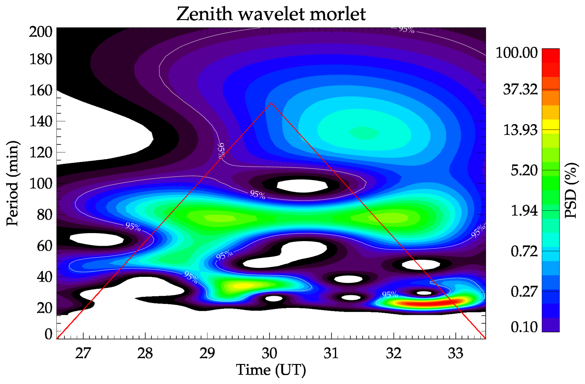
Figure 7 The wavelet power spectrum of the zenith time series for the keogram depicted in Fig. 2b illustrating all the recorded MSGW periods. The power spectrum is normalized as a percentage relative to its maximum and minimum values.

Figure 8 presents the reconstructed keogram and phase lines surrounding the temporal peaks of the 35 and 79 min waves, which appear between 29–30 and 31–33 UT. Figure 8a and c show the reconstructed keograms for the respective waves, while Fig. 8b and d depict the phase lines around the temporal peaks for the waves. Spatial and temporal changes in amplitudes appear along the keogram for both reconstructed periods. As in the simulation example, the phase lines were unwrapped. The red sections in Fig. 8b and d indicate where the optimal fit was identified (details below), aligning with the vertical red lines in Fig. 8a and c. In both components of the two reconstructions, the chosen region shows a coherent wave signal, indicating that the criteria for the best-fitting region automatically selected the phases' flattest and most parallel sections.

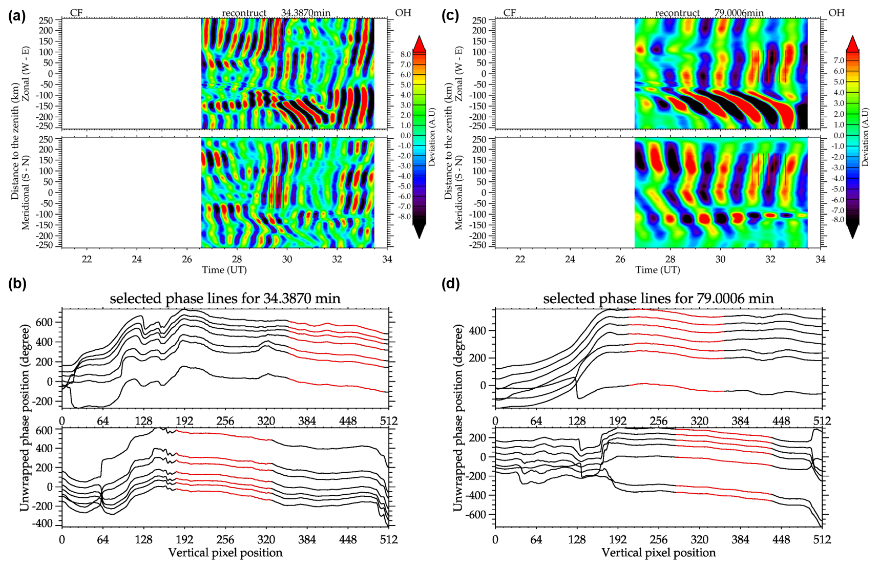
Figure 8 Reconstructed keogram for the 35 and 79 min peak periods, visible between 29 and 30 and 31 and 33 UT. The red lines depicted in panels (a) and (c) are highlighted in panels (b) and (d). They were used to calculate the MSGW parameters.

Two significant issues are evident in observed airglow keograms: (i) waves may not be present throughout the keograms; (ii) the phase lines are irregular, showing overlap between the waves. To avoid these problems, several lines are selected for a duration of half a period before and half a period after the peak central position. The phase region used in the calculation is chosen based on the fitting quality applied throughout the phase lines. This approach enables the fitting information to directly evaluate whether the signal is likely a coherent wave. A minimization threshold for the fitting variance is established to filter reliable fitting points and ensure that the signal originates from a traveling wave. Adjacent phase lines over time undergo the same fitting process and, adhering to the same minimization threshold, determine the average of the wave parameters around the peak time of the spectrum while also verifying the temporal continuity of the wave signal.

After the correct phase lines and their positions are determined, the MSGW parameters are estimated, and an average parameter is calculated from the approved phase lines if at least three phase lines meet the determined sector with fitting criteria approved, meaning the variance is below the threshold (details in Sect. 4).

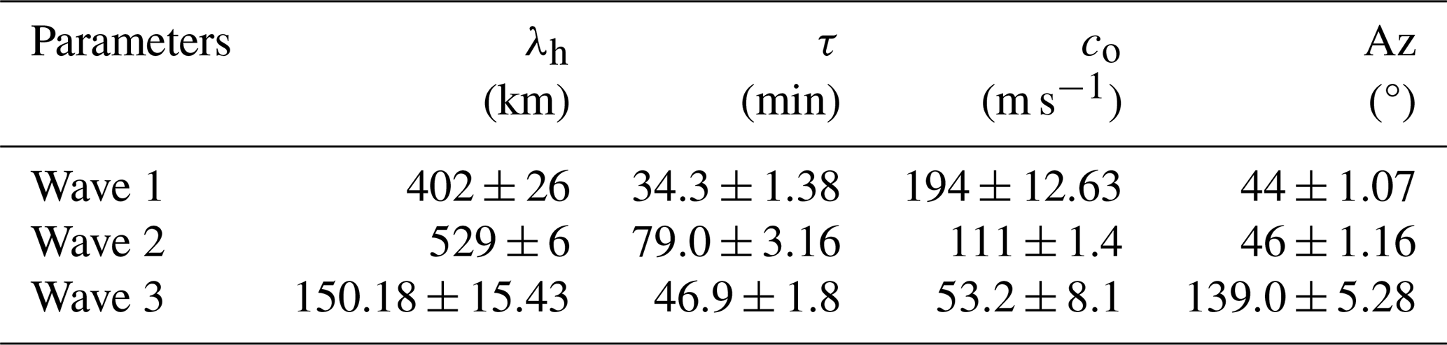
For the example used in this section, Table 2 presents the results for the night of 3–4 August 2022. The procedure approved three waves with periods of 34, 79, and 46 min. Other peaks at 134 and 22 min were identified but did not meet the fitting conditions for the phase lines. Waves 1 and 2 have tiny standard deviations from the average parameters of the approved phase lines. Although Wave 3 has more questionable results, it still remains below 15 % of the standard deviation.

Table 2 MSGW parameters obtained by the new methodology, using observed airglow images of the night of 3–4 August 2022. The uncertainties are also presented for each wave parameter.

4 Error estimations

This section examines the accuracy of the results, the error estimations, and the quality of procedures through the simulation of synthetic gravity waves. The investigation utilized the outlined procedure on a sizable dataset of simulated keograms to assess analysis quality, over error propagation throughout the process, and identify any related issues in the process. From now on, we will refer to error estimation (or propagated error) as the difference between the results of the MSGW parameter and the simulated wave parameters. It is important to emphasize that this study does not aim to validate the wavelet transform or other established mathematical procedures, such as linear fit. It still tracks errors through a combination of empirical and direct processes. Errors resulting from any transformations or mathematical procedures exist and can be studied or found in other publications. (Liu et al., 2007; Xu et al., 2024).

The dataset of simulations consisted of keograms (similar to the one presented in Sect. 2.2) with pairs of waves: a primary wave varying the parameter and a second wave with a fixed parameter. The primary wave had wavelengths ranging from 50 to 500 km in steps of 50 km, periods from 20 to 200 min in steps of 30 min, phase speeds dependent on those parameters, and propagation directions varying by 30°. A total of 819 keograms were generated. The secondary wave was set to 275 km and 90 min, propagating to 120°, and was present in all keograms. Additionally, random noise with the same amplitude as the waves was introduced. A second trial was conducted to investigate the amplitudes by varying the relative amplitude of the waves from $\mathrm{1}/\mathrm{6}$ to $\mathrm{3}/\mathrm{2}$ while keeping the directions of the primary wave constant. This was intended to assess the influence of the distance of the amplitude peak to the cone of influence (COI) on the errors.

One situation worth noting is the superposition of wave parameters during interference. Figure 9 displays the phase lines of interfering waves in the simulation results. It is important to note that the primary cause of the phase tilt's nonlinearity is the coherent presence of another wave. The lines become irregular as the waves superpose over periods or wavelengths. Amplitudes can also interfere, and a dominant wave can completely obscure a smaller one. In this scenario, the primary wave should have an 80 min period and a 200 km wavelength propagating at 120°. The result showed a 79.8 min period (the peaks were selected quite accurately), while the wavelength was 250 km, which was closer to the second simulated wave. The direction remained near the expected, 117°. This illustrates how the superposition of waves can prevent us from accurately extracting their parameters under analysis.

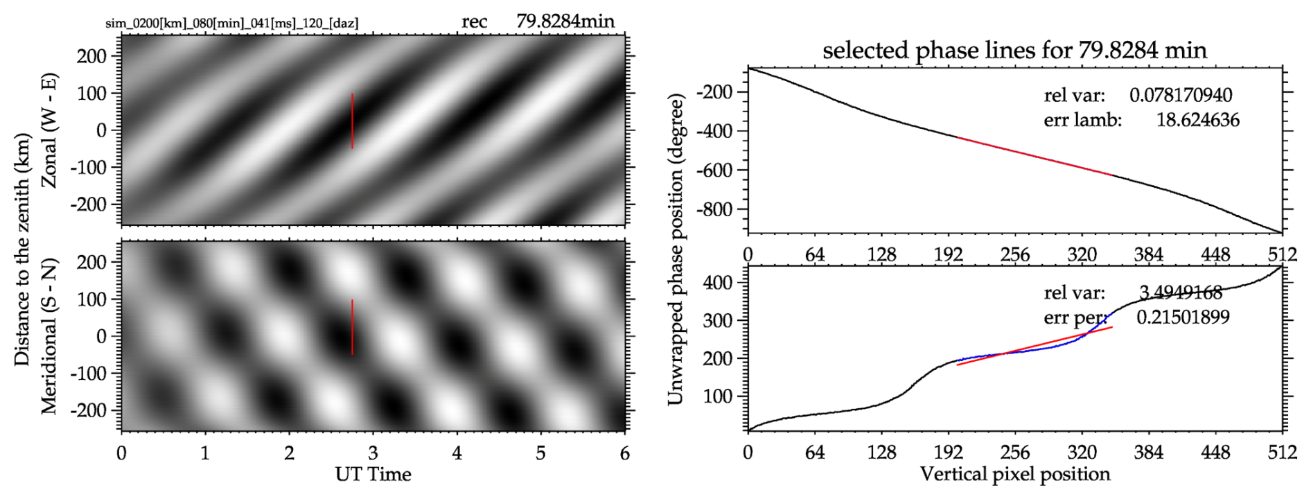
Figure 9 Two waves interfering in the simulated keogram result in tortuous phase lines, and the reconstruction resembles a chessboard pattern.

Figure 10 illustrates the errors in the calculated MSGW parameters as a function of the variance of the angular parameters in the linear fit. The straight red line passes through the points (0,0) and (1,15), but it appears curved because of the log scale on the x axis. Numbers inside each plot indicate the number of waves over 15 % of the error relative to a maximum threshold (in this case, it equals one). An almost linear growth of the errors with amplitude is observed with the variance increase, except for the periods and amplitudes that follow a regular value. Deviations in the periods stem from the inherent limitations of the wavelet transform, while amplitudes will be addressed later. One key pattern to note is the potential cutoff value for the variance, which ensures proper wave selection and accurate parameter estimation. For the example provided, this threshold might be set at one. Still, it must be adapted for each scenario due to its sensitivity to the prior processing, signal-to-noise ratio, and data resolution.

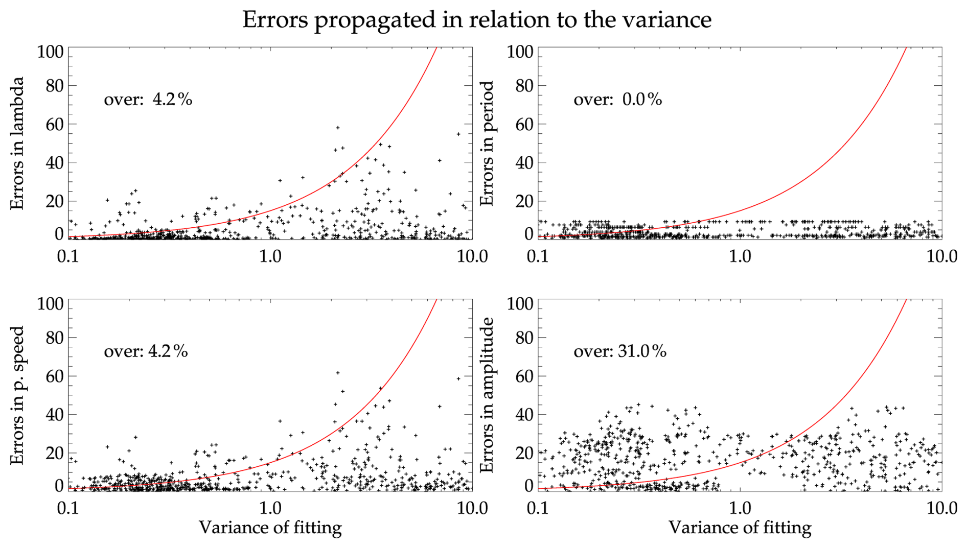
Figure 10 Estimated errors for the simulated MSGW parameters as a function of the variance of the linear fit applied to the reconstructed phase lines.

Amplitude correction presents challenges because of the numerical limitations of wavelets, and even after correction, persistent issues remain. The primary concern is wave superpositions, and a noticeable reduction occurs when the spectrum's peak falls outside the COI. The amplitudes were assessed individually to understand why their errors were significantly larger than those of other parameters. As the amplitudes do not require passing through the phase line identification, their errors were assessed based on the position of the amplitude peak concerning the COI. The findings indicate that peaks within the COI have an estimation error of less than 10 %, whereas peaks outside the COI may have an error of up to 20 %. This addresses the issue of peaks that fall outside the COI. No significant errors were identified in the MSGW parameters for the selections made outside the COI, aside from amplitudes that escalate errors to approximately 20 %.

Figure 10 illustrates the quasi-linear progression of errors with variance. Furthermore, a statistical distribution can be defined, with the mean error value and the variation from this mean for the results that fell below the threshold. Table 3 presents the average error values obtained from the simulations, constrained by the discussed threshold. Apart from the amplitudes previously discussed, the error values do not increase significantly below the threshold.

Table 3 The average results from the error propagation study conducted through simulations and the standard deviation σ of the distributions shown in Fig. 10.

5 Results of the MSGW observed in Antarctica

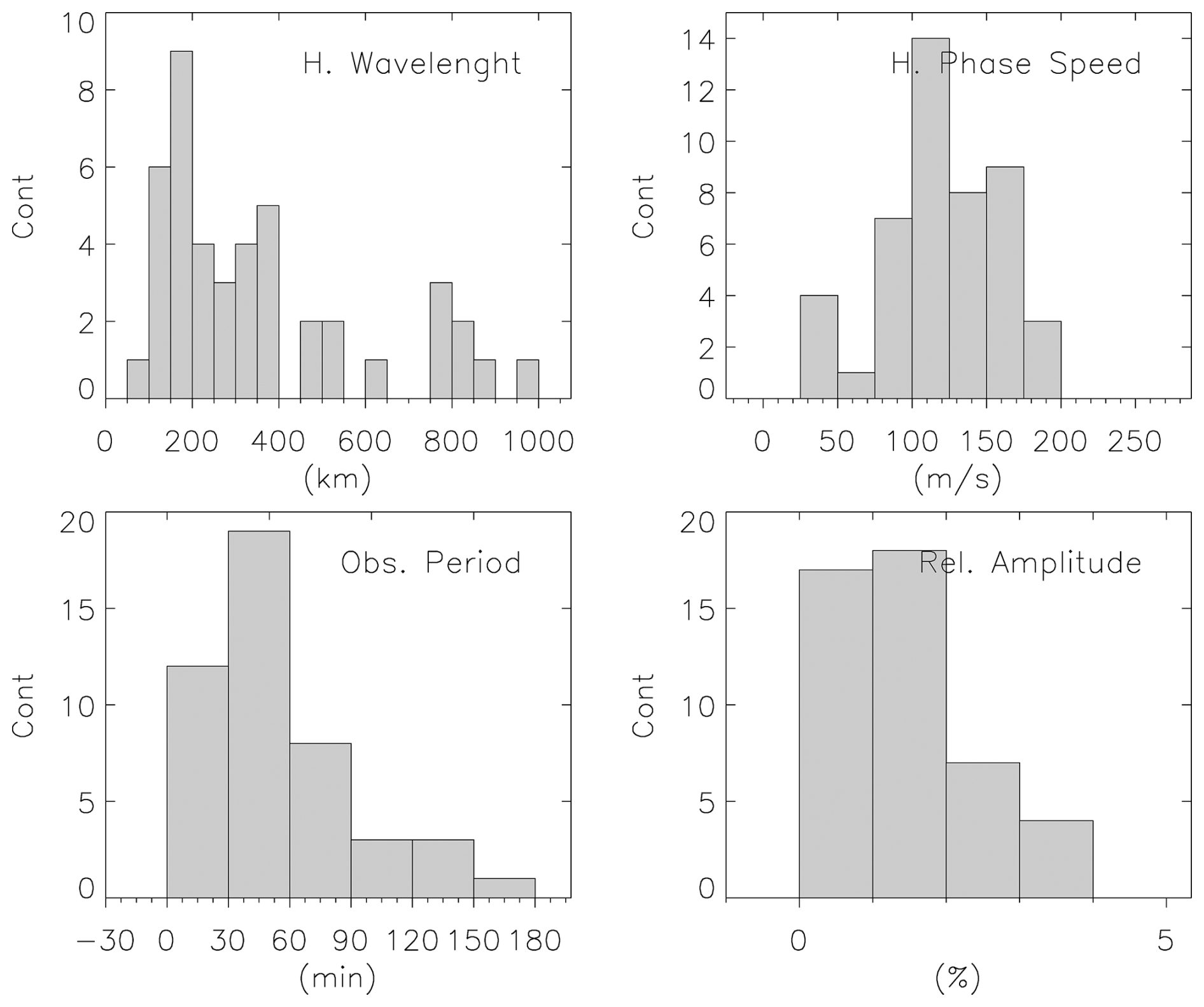
In 2022, an all-sky airglow imager was operated in Antarctica, taking images on nights when the Moon was not visible. To study medium-scale gravity waves and achieve reliable results, only observation periods exceeding 2 h were utilized. This approach ensures that the observed waves remain near the COI of the wavelet results, thus eliminating any bias in amplitude estimation. In line with this concept, 18 nights were chosen for analysis, resulting in 46 medium-scale gravity waves examined using the outlined methodology.

Histograms of the calculated MSGW parameters are presented in Fig. 10. The histogram of the observed horizontal wavelengths appears in the first panel, while the second and third panels display the histograms of the observed periods and phase speeds. The last panel displays the relative amplitudes of the waves; specifically, the amplitudes obtained from the wavelet analysis divided by the mean background brightness of the images. In addition to a wide range of wavelengths from 100 to 1000 km, most waves had wavelengths less than 400 km. The periods peaked at 20 to 90 min (with 20 min being the minimum value accepted in the analysis), and in some cases, they extended to nearly 180 min. Phase speeds peaked between 75 and 200 m s⁻¹, accompanied by some slower waves. Amplitudes remained below 4 % with a concentration under 2 %; these waves are faint oscillations.

Figure 12 illustrates the propagation directions of the waves as a function of their respective phase speeds, or their phase velocity vectors. Waves across a broad spectrum of velocities propagate in all directions without apparent anisotropy. However, more waves are observed with zonal components predominantly in the eastward direction compared to the westward direction. Additionally, no wind filtering pattern could be identified.

Figure 11 Histograms of the MSGW parameters observed at Antarctica in 2022.

6 Discussions of the methodology and MSGW results

This work describes a new methodology to determine medium-scale gravity wave parameters observed in a keogram automatically. Although it is consistently based on previous methods, we highlight the new features here: using the wavelet instead of the FFT to identify the timing of the waves, verifying the wave signal based on the wavelet's properties, and employing an automatic procedure with no human interference throughout. We identify as limitations the reliance on the fitting of linear phase lines and the necessity for meticulous human approval of the results after the process is concluded.

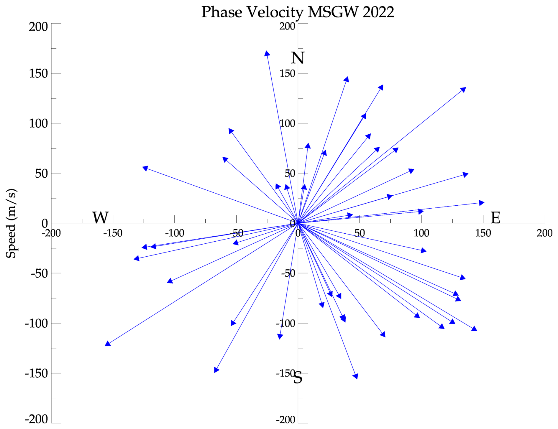
Figure 12 Phase velocity vectors of the analyzed MSGW. Each blue arrow is one MSGW phase velocity vector.

Additionally, this procedure addresses two common issues identified in the analysis: the waves are typically absent from some regions of the keogram and often interfere with noise and other waves. The superposition of waves is unavoidable, which represents a fundamental issue in oscillator theory. When specific wave properties, such as period, wavelength, or direction, are very similar, the resulting outcome may be a mixture of the two waves, as confirmed in our error propagation study through simulations. The threshold applied to the fitting deviation of phase lines and the multiple, time-spaced phase lines effectively minimized the impact of noisy and overlapping waves. However, we could still guard against these issues by visually inspecting the reconstruction to verify the presence and coherence of the waves, a capability lacking in earlier methods.

In Fig. 10, the spectrum exhibits numerous higher error values resulting from the ambiguous selection of wave properties during wave interference. The resulting period can be closer to one wave, while the resulting wavelength is nearer to another. As shown in Fig. 9, the analysis identified the period of one wave but the wavelength of another, creating visually tortuous phase lines. These conclusions led us to believe that an accurate selection of the waves must come after verifying the reconstruction of the phase line and ensuring there is no tortuous signal in those phase lines.

To emphasize the progress in the presented methodology, Fig. 13 displays the results of the previous method for comparison and discussion. Panel (a) presents the keogram utilized for the analysis, whereas panels (b) and (c) illustrate the results for waves 1 and 2. The upper panels illustrate the chosen human-oriented region, while the lower panels display the power spectrum for the components along with the analysis results. Further information regarding the method is available in Nyassor et al. (2025). Besides its simplicity, it is based on the FFT and the cross-spectra to obtain the phase difference along the lines. The program operator should choose the region of interest and verify if the results align with their observations. For instance, they need to confirm that the phase fronts are closely spaced in accordance with the result period and that their tilts correspond to the resulting propagation direction.

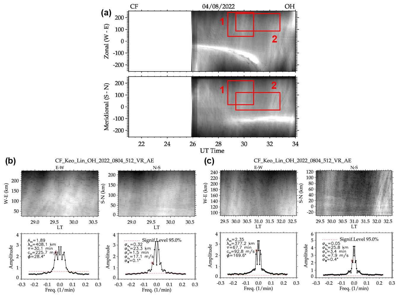
Figure 13 Example of the results of MSGW calculated using the previous methodology. In panel (a), a keogram is used for the analysis: red boxes highlight the human-selected region for analyzing waves 1 and 2. The resulting images are presented in panel (b) for the Wave 1 analysis and in panel (c) for the Wave 2 analysis. The upper panels in the results display the selected regions, while the lower panels present the power spectrum plots and MSGW results with associated errors.

In comparison to the newly developed method, we emphasize the following points as significant enhancements to the methodology. The operator is not required to visually inspect the chosen areas to assess the reliability of the expected MSGW propagation direction. The outcome reflects the new model's reliability, as demonstrated by the reconstruction quality thoroughly analyzed and illustrated in Fig. 10. Avoiding the Milky Way is a concern that the operator must be cautious about; the phase line selection in our procedures indicates that it automatically avoids the Milky Way, which disrupts the phase continuity.

It has been observed that the previous analysis did not use the higher peak in the power spectrum. Indeed, the operator can select the wave that they want; in the first case, the peak is the 60 min wave, while the second identifies the 135 min wave. Neither analysis was applied to the higher wave peak in the spectrum. Altering the selected region can modify the displayed parameters. This results from the superposition of the waves, an issue that remains in the new method. As mentioned in the section on errors, while accurately identifying peaks and distinguishing the wave from the background (which may include other waves) is important, parameter mixing can still occur, and there might not be effective solutions. In addition, our innovative method automatically identifies and displays the key periods in the keogram separately and provides an associated evaluation, indicating the result quality better.

Different regions were selected in the keogram components for each wave, sometimes far from the zenith. The authors believe that because the waves are medium-scale waves, their dimensions are large enough to be present to a significant extent in the images and, consequently, in the keograms. In the previous methodology, the operator must carefully select the same wave on both keogram components. In the new methodology, we could configure the program to steer clear of selecting phase lines near the borders, yet we opted to allow the code to independently identify the wave packet. Nonetheless, results have consistently demonstrated strong performance in this region.

Finally, we assume that the simulated waves, shown in the synthetic images, propagate the same errors as observed waves in the airglow images when considering their discrete signal. In conclusion, the error estimation determined in the simulations is used as the inherent error propagated in the analysis. It will be applied in future works on the observed airglow images for MSGW studies. Errors in phase speed are inherently more significant due to error propagation. Regarding the peaks outside the COI of the power spectrum, no major errors were identified in the MSGW parameters for selecting the peak, except for the amplitudes, which show consistent errors of around 20 %. While these errors are notable, the overall methodology remains highly satisfactory and achieves impressive results similar to earlier methods. Additionally, it may help minimize user bias by automating much of the process.

In the tropical region of Brazil, medium-scale gravity waves were observed by Taylor et al. (2009) using airglow imaging with a different methodology. Their results showed waves with horizontal wavelengths ranging from 50 to 200 km, observed periods of 20 to 60 min, and horizontal phase speeds of between 20 and 80 m s⁻¹, which were smaller and more concentrated than ours. Most of their waves were moving southeast and east. In the equatorial region, Essien et al. (2018) observed a significant number of MSGWs applying a Fourier transform. Their results showed waves ranging from 50 to 250 km with periods of 20 to 80 min and speeds of between 20 to 120 m s⁻¹, with the majority of the MSGWs moving north and northeast. They also observed strong anisotropy in the propagation directions related to wind filtering. Gravity waves observed in this study differ from those in other locations, primarily with respect to phase speed and wavelength distribution. The phase speed showed a broader distribution with higher values. The wavelengths exhibited a more extensive peak distribution, including a secondary peak around 800 km, which, to the authors' knowledge, has not yet been reported in airglow observations. In addition to some differences in the observed parameters, the results of our newly developed method agree with prior observations; the differences may be attributed to regional medium-scale gravity wave characteristics.

The amplitudes of medium-scale gravity waves observed by airglow imagers have not been previously addressed. Vargas et al. (2021) examined waves with periods comparable to ours directly in airglow images and estimated the amplitudes of waves under 50 min, generally showing relative amplitudes of less than 5 %; their findings agree with our observations. Medium-scale gravity waves have small amplitudes; this seems reliable because they are tenuous oscillations on the background of small-scale gravity waves. Thus, the present study could identify those faint waves through the applied image processing and distinguish overlapping waves by the phase line identification. At the same time, the work mentioned did not attempt to separate overlapping waves.

7 Conclusions

A new analysis methodology was developed for medium-scale gravity wave (MSGW) observations using keograms from airglow images. This method relies on wavelet transform, leveraging its characteristics to extract wave parameters efficiently while minimizing issues related to error propagation. The wavelet amplitudes were adjusted to ensure accurate wave amplitude measurements.

Simulated medium-scale gravity wave images were utilized to verify the error propagation throughout the procedure and to ensure reliable wave parameter estimation. Error propagation is minimal for all gravity wave parameters except the amplitudes, which, despite their correction, can still be underestimated when the peak lies outside the power spectrum cone of influence.

The MSGW parameters observed in Antarctica showed the typical behavior of medium-scale gravity waves observed at other sites using different methodological analyses. Overall, the newly developed methodology demonstrated remarkable effectiveness with respect to wave identification and parameter estimation while also minimizing user bias, which was typically prominent in earlier approaches. A drawback of the method lies in its reliance on a threshold for fitting quality estimation, which is influenced by image processing and data resolution. However, this has been demonstrated not to limit the method itself or the quality of the results. Despite its shortcomings, the new methodology can be utilized to analyze MSGWs in other airglow observations from different locations across the Antarctic continent, an initiative that is currently underway.