The saturation vapor pressures of higher-order polyethylene glycols and achieving a wide calibration range for volatility measurements by FIGAERO-CIMS

The Filter Inlet for Gases and AEROsols coupled with a Chemical Ionization Mass spectrometer (FIGAERO-CIMS) is a widely used method for determining the chemical composition of the molecular constituents of atmospheric organic aerosols (OA). This temperature-programmed desorption technique thermally desorbs OA in a linearly ramped desorption temperature, and the temperature at a detected molecule's peak desorption rate, T_max, is proportional to the molecule's volatility. Thereby, FIGAERO-CIMS also enables a direct measurement of the volatilities (saturation vapor pressures) of the OA constituents. A series of polyethylene glycols (PEGs) has been used to quantitatively connect FIGAERO measurement results (in particular, T_max) to volatilities (i.e., calibrate). However, available literature values of saturation pressure (P_sat) or saturation mass concentration (C^*) for these compounds only extend to PEG 9, which exhibits T_max values around ∼ 90 °C, whereas T_max values of OA constituents measured from lab-generated or ambient aerosols routinely reach up to 160 °C (Li et al., 2021; Masoud et al., 2022). To extend the region over which we can conveniently calibrate FIGAERO-CIMS, and hypothetically also other thermal desorption-based techniques for investigating OA composition and volatilities, we performed FIGAERO-CIMS calibration experiments using aerosol particles consisting of PEGs 5-15, which yielded T_max values of up to ∼ 150 °C. We then set out to estimate the hitherto unknown P_sat (C^*) values of PEGs 10-15 by utilizing a suite of different P_sat estimation methods: both measurement-independent methods (quantum chemistry-based calculations, molecular structure-based group contribution methods, and parametrizations based on molecular sum formulas) and fits of an explicit desorption model to our FIGAERO measurement results with C^* and vaporization enthalpies as free parameters. We assess the respective suitability of each method and argue that we obtain the best estimates for PEG volatilities based on the fits to our measurements. We obtained log ₁₀(C^* (µg m⁻³)) values ranging from 0.51 ± 0.07 (PEG 6) to −9.2 ± 1.6 (PEG 14), agreeing with previous literature results on PEGs < 10. Within uncertainties, our results broadly continue the near log-linear relationship of C^* with PEG mass for larger PEGs and also agree with some of the independent methods. Contrary to common assumptions in previous literature on FIGAERO results, we find that the relationship between ${\log }_{\mathrm{10}}\left(C^{*}\right(\mathrm{\mu }\mathrm{g}{\mathrm{m}}^{-\mathrm{3}}\left)\right)$ and measured T_max is not linear. We explore the consequences of this finding on the analysis of previously published FIGAERO-CIMS measurements of sesquiterpene-derived OA. Prospects for improving on our results in future work are discussed. We conclude that calibration experiments using aerosol containing PEGs up to ∼ PEG 15, with best-estimated saturation vapor pressures, provide promising opportunities for constraining the volatilities of aerosol constituents, down throughout the range of extremely low-volatility organic compounds (ELVOC, C^* < 3 × 10⁻⁴ µg m⁻³), as detected not only via FIGAERO-CIMS but also other (online) temperature-programmed desorption techniques.

1 Introduction

Aerosol particles are an important factor in air pollution and the atmosphere's radiation balance. Much of this suspended particulate mass consists of organic material, often constituting most aerosol mass in the sub-micron size range that is particularly relevant for providing cloud condensation nuclei (thereby affecting indirect radiative forcing; Sporre et al., 2020). Chemically, that organic aerosol fraction has turned out to be extremely complex, and it remains a great challenge to determine the detailed chemical composition of organic aerosol (OA). That is due to the diversity of organic species present in our atmosphere. Their complex chemical processing in the gas phase largely determines their propensity to condense into aerosol particles, while condensed-phase reactions may further alter OA composition, subject also to inorganic constituents (including water) and physical aerosol properties such as viscosity (Hallquist et al., 2009). All these properties may also affect the volatility of OA, i.e., its proclivity to evaporate in response to changes in its chemical and physical environment (e.g., the removal of condensing species from the gas phase or changes in temperature). OA volatility is thus a key property for describing aerosol evolution and lifetime under changing environmental conditions. Among the state-of-the-art mass spectrometry-based methods to tackle these measurement challenges related to OA – in particular measurements of both elemental composition of OA constituents and their volatilities – is the Filter Inlet for Gases and AEROsols (FIGAERO, Lopez-Hilfiker et al., 2014), coupled to a time-of-flight chemical ionization mass spectrometer (ToF-CIMS) that is sensitive to a wide range of organic compounds that are present in the atmosphere in trace amounts, including compounds forming OA (Bertram et al., 2011). The FIGAERO-CIMS is a semi-online method, with two alternating modes of operation: aerosol is collected on a polytetrafluoroethylene (PTFE) filter while the CIMS measures gas-phase compositions; then the gas inlet is blocked while a gradually heated nitrogen (N₂) flow desorbs the collected aerosol particles and the resultant thermally desorbed vapours directly enter the CIMS for composition measurements (details in Sect. 2.2).

FIGAERO-CIMS instruments have been successfully employed in numerous studies of OA over the last decade (Thornton et al., 2020). The instrument can, with some caveats, identify and quantify both gas-phase and particle-phase chemical compounds over a broad range of chemical functionalities (Lopez-Hilfiker et al., 2014). The inbuilt controlled thermal desorption mechanism also allows investigating the volatilities of the compounds detected from the particle phase. Such particle volatility measurements using FIGAERO-CIMS rely on the accurate identification of the so-called T_max values of individual compounds, i.e., the temperatures at which the highest respective signals are observed. These T_max values are inversely proportional to volatility and can be converted to saturation vapor pressure P_sat and saturation mass concentration C^* values, as has been shown empirically and through modelling (Lopez-Hilfiker et al., 2014; Schobesberger et al., 2018). However, an accurate conversion from T_max to P_sat and C^* would require a reliable calibration (Bannan et al., 2019; Ylisirniö et al., 2021).

Unfortunately, due to a lack of calibration compounds with known P_sat at low volatilities (P_sat < 10⁻⁹ Pa $/$ C^* < 10⁻⁴ µg m⁻³), the current calibration procedure can only cover the desorption temperature range up to ∼ 80–100 °C, but desorption temperatures of FIGAERO-CIMS can reach 200 °C and for ambient or lab-generated OA, T_max values are routinely identified up to 160 °C. In this study, we aim to extend the calibrated range of FIGAERO-CIMS for P_sat measurements to also cover lower P_sat values down to P_sat ∼ 10⁻¹⁶ Pa $/$ C^* ∼ 10⁻¹¹ µg m⁻³. We utilize a combination of different methods to improve the accuracy of estimating saturation pressures of low-volatility compounds. The core of our study is careful FIGAERO-CIMS calibration experiments using a wide range of polyethylene glycol (PEG) polymers from PEG-5 to PEG-15. The experiments are supported by parametrization and modelling approaches for assessing the P_sat that have so far remained uncertain for PEGs beyond an order of 9 (PEG-9; P_sat ≈ 6.7 × 10⁻⁹ Pa; Krieger et al., 2018; Li et al., 2023). Note that all P_sat or C^* discussed in this study refer to the equilibrium pressures (concentrations) over the pure (partly assumed) liquid substance, unless stated otherwise.

2 Materials and methods

2.1 Generation of calibrant aerosol

We generated calibrant aerosol particles by atomizing a solution containing PEG polymers, H-(O-CH₂-CH₂)_n-OH, ranging from an order of n = 5 (PEG-5) to 15 (PEG-15) using a Topas ATM 226 atomizer. Individual PEGs were obtained from Polypure AS (≥ 95 % purity). The used solvent was acetonitrile (ACN) (Fisher Scientific, 99.8 % purity). The initial concentration of each PEG in the solution was ∼ 0.2 g L⁻¹. Note that the concentration of each individual PEG increases during the atomization process as the solvent has a higher vapor pressure than the PEGs. All PEGs were dissolved into the same atomization solution. The atomized polydisperse particles were directed through a dilution system to ensure the evaporation of ACN (Ylisirniö et al., 2021). We then size-selected 100 nm electrical mobility-sized monodisperse particles from the “dried” polydisperse particles using a differential mobility analyser (TSI 3080). The resulting monodisperse particles were then directed to both the FIGAERO filter collector and a condensation particle counter (CPC, TSI 3775) via a flow splitter.

2.2 FIGAERO-CIMS

The ToF-CIMS (Tofware AG, Aerodyne Research Inc.) was operated with an iodide-ionization scheme (Iyer et al., 2017; Lee et al., 2014). The mass resolution of the instrument was 4000–5000 over the relevant mass range. Iodide ions were generated by passing an ultrapure N₂ flow of 1 standard L min⁻¹ over a permeation tube containing methyl iodide (CH₃I, Sigma Aldrich 99 % purity), followed by a commercial Po-210 α-radiation source (Model P-2021, NRD Static Control LLC). The formed I- ions were fed into the Ion Molecule Reaction (IMR) chamber, where they mixed with a 2 L min⁻¹ flow of sample molecules. The IMR chamber was actively controlled to a pressure of 100 mbar and actively heated to 60 °C with heating wires wrapped around the outside of the IMR to accomplish even heating.

The operation of the FIGAERO inlet is thoroughly explained in previous publications (Bannan et al., 2019; Lopez-Hilfiker et al., 2014; Thornton et al., 2020). Briefly, the FIGAERO inlet enables measurements of both gas-phase and particle-phase chemical constituents through two separate pinholes leading into the instrument. In normal operation, the gas-phase vapours are directly sampled into the IMR, while the other pinhole is kept closed, and aerosol particles are sampled onto a PTFE filter (SKC Inc. PTFE membrane filter, pore size 2 µm, 25 mm diameter, of which a central section of 6 mm diameter is exposed to sampling flow). Once a sufficient amount of particulate matter (typically ∼ 100–200 ng) has been collected onto the PTFE filter, the filter is moved over the second pinhole, and the gas phase sampling pinhole is closed. Chemical constituents are then evaporated from the aerosol particles collected onto the filter by a gradually heated ultra-pure N₂ flow through the filter and into the IMR (2 standard L min⁻¹). The heating cycle of the FIGAERO typically consists of two phases, the so-called heat ramp phase and soak phase. During the heat ramp phase, the N₂ is heated from room temperature linearly to ∼ 200 °C, as measured a few millimetres above the filter. This is followed by the soak phase, where the N₂ flow is maintained at 200 °C to evaporate any remaining material from the filter. The measurement data used in this study was selected from two sets of measurements, a first set in January 2022 (experiments A and B) and a second set in July 2022 (experiment C). In experiments A and B, we used ramping times of 5 and 15 min with particulate mass loadings of 105 ng and in experiment C, we used a 10 min ramping time with particulate mass loading of 170 ng, based on calculations from CPC readings while assuming spherical particles and a density of 1.125 kg m⁻³ (Krieger et al., 2018). Note that the mentioned aerosol mass loadings refer to the total collected mass over all PEG compounds. Collected masses of individual PEGs ranged from ∼ 5 to 10 ng per compound. The used collection flow was 1 L min⁻¹ in all experiments. Additional blank heating cycles with no collected particles were also performed before individual experiments to ensure and confirm low background signals. Details of these measurements are further discussed in Sect. 3.3.

In this study, we employed a custom-built version of the FIGAERO inlet, which slightly differs from the commercially available FIGAERO inlet produced by Aerodyne Inc. These differences are mainly in the control program and electronics used, but the main measurement principles are the same.

Data-analysis

The time-of-flight data was processed using the tofTools software package (Junninen et al., 2010) written in MATLAB (Mathworks Inc.) and further post-processed with custom MATLAB scripts. The data-analysis procedure follows the outline stated in Ylisirniö et al. (2021). Briefly, both CIMS data and temperature data were recorded in 1 Hz time resolution and averaged to 0.2 Hz resolution in the preprocessing. CIMS data was then compared against the temperature data to form so-called thermograms (i.e., ion count rates, proportional to the PEGs' desorption rates, vs. desorption temperature). In the typical case, these thermograms resemble a lognormal function. The peak value of the thermogram is called T_max (i.e., the temperature of maximum desorption). For obtaining theT_max values from the thermograms, an asymmetrical lognormal function was first fitted to the measurement data and T_max values were assigned to the maxima of these functions, thus minimizing the impact of noise on those assignments.

Obtained T_max values of individual compounds have previously been found to follow a log-linear relationships against literature-values of saturation vapor pressure P_sat,lit of said compound (Bannan et al., 2019; Lopez-Hilfiker et al., 2014; Ylisirniö et al., 2021), following the equation

$$\begin{array}{}\text{(1)}& \ln \left(P_{\mathrm{sat},\mathrm{lit}}\right)=a{T}_{max}+b,\end{array}$$

where a and b are fitted parameters. Saturation vapor pressure values of any other measured compounds could be then estimated with the equation

$$\begin{array}{}\text{(2)}& P_{\mathrm{sat},\mathrm{meas}}=e^{a{T}_{\max ,\mathrm{meas}}+b},\end{array}$$

where T_max, meas is the measured T_max value of the compound of interest. It is often customary in the field of aerosol science to express P_sat values as C^*, which can be calculated using the ideal gas law:

$$\begin{array}{}\text{(3)}& C^{\ast }\left(\mathrm{\mu }\mathrm{g}{\mathrm{m}}^{-\mathrm{3}}\right)={\displaystyle \frac{P_{\mathrm{sat},\mathrm{meas}}{M}_w}{RT}}{\mathrm{10}}^{\mathrm{6}},\end{array}$$

where M_w is the molecular weight of the compound (in units of g mol⁻¹), R is the universal gas constant (8.314 J mol⁻¹ K⁻¹) and T is the temperature (in units of K) of which the literature P_sat,lit value was determined (in our case, 298 K).

Ylisirniö et al. (2021) further suggested to accomplish the linear fit of Eq. (1) using a bivariate least squares method (York et al., 2004), e.g., as implemented in MATLAB by Pitkänen et al., 2016, to account for uncertainties in the determination of both P_sat, lit and T_max, meas.

2.3 Saturation vapor pressure determination

The volatility calibration of FIGAERO-CIMS presented here relies on the known saturation vapor pressure values of the PEGs in order to determine the calibration parameters via Eq. (1) (Ylisirniö et al., 2021). Literature values of P_sat for PEGs are available for PEG-1 to PEG-9 (Krieger et al., 2018, later abbreviated to K2018. Li et al., 2023, later abbreviated to L2023).

Experimental data thus exist in literature for P_sat of PEG-1 to PEG-9, but reference data for larger PEGs (PEG-10 to 15) are missing. To extend the volatility range to lower volatilities, we determine the P_sat values of PEGs 5 to 15 with several different modelling and parameterisation methods based on either the molecular composition or measured thermograms. The estimation methods that are based on molecular composition range from simple molecular formula-based parametrisations (Li et al., 2016; Mohr et al., 2019; Peräkylä et al., 2020; Stolzenburg et al., 2018) and functional group-based methods (Modified Grain Model, EVAPORATION, SIMPOL) to a more detailed molecular structure-based quantum chemical model (COSMO-RS; Eckert and Klamt, 2002; Klamt, 1995; Klamt et al., 1998). We also use fits of a desorption model (Schobesberger et al., 2018) to the experimental thermograms with P_sat values as free parameters. These methods are more thoroughly discussed in the following subsections.

2.3.1 Desorption modelling

The desorption model was specifically developed to simulate the thermal desorption of filter-collected aerosol particles in the FIGAERO and transport into the CIMS, details seen in Schobesberger et al. (2018). In our study here, the model was set up with a minimal number of free parameters, which are explained later in this section. Model runs used as input the desorption temperature ramp rates as used experimentally and monodisperse aerosol particle sizes as classified (Sect. 2.2). The simulated particles initially consisted of the involved PEGs in equal molar amounts. No chemical reactions (i.e., no oligomerization, decomposition, etc.) were allowed, and the particles were assumed to always be homogeneous ideal mixtures. In Schobesberger et al. (2018), possibly delayed detection by an older-generation FIGAERO had been attributed to interactions between desorbed molecules and instrumental surfaces. These delays/interactions were disabled here, i.e., simulated detection of molecules was simultaneous with their simulated desorption from the particles. Non-ideal heating was assumed, using the same parametrization as in Schobesberger et al. (2018), which served to provide the observed “tails” in the thermograms, while having a minimal effect on the simulated T_max. The only free parameters were the saturation vapor pressure (P_sat, i) and vaporization enthalpy (ΔH_i) of each PEG i, and the sensitivities of the CIMS to each compound (S_i). These parameters were fit to the observations, wherein ΔH_i were primarily constrained by the thermograms' upslopes, P_sat, i by ΔH_i and $T_{max,i}$, and S_i by the thermogram height (i.e., amount of signal).

To provide uncertainties for those fit parameters, while accounting for variabilities between individual experiments, we applied an automated model optimization algorithm 24 times to a representative selection of three individual experiments (A, B, C), thus exploring the sensitivity of the quality of the fit to each parameter and experiment. Further discussion of that procedure and its results are discussed in Sect. 3.3.

2.3.2 Conductor-like screening model for real solvents (COSMO-RS)

We used the COSMOtherm program (BIOVIA COSMOtherm, 2021) to estimate saturation vapor pressures of PEGs 5-8, 10, 12 and 14. COSMOtherm is based on the conductor-like screening model for real solvents (COSMO-RS), which is a quantum chemistry-based model that considers the exact structure (specific structural isomer and even the geometry of the most stable conformation in the gas and condensed phase) of molecules in saturation vapor pressure calculations. In COSMOtherm, P_sat is calculated using

$$\begin{array}{}\text{(4)}& P_{\mathrm{sat},i}=\exp \left({\displaystyle \frac{G_i^l-G_i^g}{RT}}\right),\end{array}$$

where the free energies (G) in gas (g) and pure condensed (l) phase are derived from density functional theory (BP/def2-TZVPD-FINE//BP/def-TZVP level of theory). The conformer selection for our COSMOtherm calculations is detailed in Sect. S1 of the Supplement.

2.3.3 Modified Grain Method (MGM)

The modified Grain method (MGM) is an estimation of vapor pressure based on the boiling point of a compound, as determined by a structure-activity relationship based on Stein and Brown (1994) and others' work (Joback, 1984; Reid et al., 1959). The boiling point is calculated by the following

$$\begin{array}{}\text{(5)}& T_{\mathrm{b}}=\mathrm{198.2}+\sum \left(n_i\times g_i\right),\end{array}$$

where T_b is the boiling temperature in Kelvin, g_i is the group increment value, and n_i is the number of those functional groups present in the molecule. The boiling point (if it is calculated to be less than 700 K) is then corrected using the following equation:

$$\begin{array}{}\text{(6)}& T_{\mathrm{b}\mathrm{\_}\mathrm{c}}=T_{\mathrm{b}}-\mathrm{94.84}+\mathrm{0.5577}\times T_{\mathrm{b}}-\mathrm{0.0007705}{\left(T_{\mathrm{b}}\right)}^{\mathrm{2}},\end{array}$$

where T_{b_c} is the corrected boiling point (K). The relationship between boiling point and functional groups was based on the analysis of 4426 organic compounds. Once the boiling point is estimated (if not already available from previous measurements), this temperature is used to calculate the liquid vapor pressure through the following equation:

$$\begin{array}{}\text{(7)}& \begin{array}{rl}\ln \left(P_{\mathrm{l}}\right)& ={\displaystyle \frac{K_{\mathrm{F}}\ln \left(R{T}_{\mathrm{b}}\right)}{\mathrm{\Delta }{Z}_{\mathrm{b}}}}\\ & \times \left[\mathrm{1}-{\displaystyle \frac{{\left(\mathrm{3}-\mathrm{2}{T}_{\mathit{\rho }}\right)}^m}{T_{\mathit{\rho }}}}-\mathrm{2}m{\left(\mathrm{3}-\mathrm{2}{T}_{\mathit{\rho }}\right)}^{m-\mathrm{1}}\ln \left(T_{\mathit{\rho }}\right)\right],\end{array}\end{array}$$

where ln (P_l) is the natural logarithm of the liquid vapor pressure, K_F is a structural factor (Lyman et al., 1990; Mill and Mabey, 1985), R is the gas constant, ΔZ_b is the compressibility factor (0.97), T_b is the estimated normal boiling point as estimated in Eqs. (5) and (6), T_ρ is equal to $T/T_{\mathrm{b}}$, where T is the reference temperature (298 K), and m is equal to 0.4133 − 0.2575T_ρ.

Additional structural factors have been introduced since the publication of Stein and Brown (1994), and have been incorporated into EPIWIN, the program we used to estimate the vapor pressures with the modified grain method. A complete list of structural factors and corrections are reported in the freely available program (US EPA, 2024) in addition to previous publications (Lyman et al., 1990; Stein and Brown, 1994).

2.3.4 EVAPORATION and SIMPOL

The “simplified p${}_L^o$ prediction method” SIMPOL (Pankow and Asher, 2008) and EVAPORATION (Estimation of VApour Pressure of ORganics, Accounting for Temperature, Intramolecular, and Non-additivity effects; Compernolle et al., 2011) are popular methods for predicting the (subcooled) liquid saturation vapor pressures of organic compounds based on their molecular structures. SIMPOL uses the basic group contribution approach: the logarithm of the saturation vapor pressure is described as the sum of terms that amount to the individual contributions of features of the molecular structure (“groups”). SIMPOL considers a total of 30 possible groups. The group contribution terms are temperature-dependent with empirically determined coefficients based on 272 compounds. EVAPORATION uses a more complex description of the molecular structure, with empirically determined parameters based on 579 compounds. The model can be run, for example, on a website https://tropo.aeronomie.be/models/evaporation (last access: 27 March 2025); requiring as input the molecular structure using the Simplified Molecular Input Line Entry Specification (SMILES), and temperature. Like all P_sat values reported in this study, the P_sat values calculated via SIMPOL and EVAPORATION are based on a temperature of 298 K.

2.3.5 Elemental composition parametrizations

We used three volatility parametrizations based on molecular formula: those suggested in Li et al. (2016), Mohr et al. (2019), Peräkylä et al. (2020) and Stolzenburg et al. (2018). Each of them uses the number of carbon, hydrogen, oxygen and nitrogen (C, H, O and N) atoms from the sum chemical formula of the compound to predict the compound's volatility. Equations of each parametrization are presented below. Note that these parametrizations yield saturation vapor concentrations (C^*) rather than vapor pressures (P_sat). See Eq. (3) for the conversion between these quantities.

The Li et al. (2016) parametrization (later, L2016) for compounds containing C, H and O atoms is of the form

$$\begin{array}{}\text{(8)}& {\log }_{\mathrm{10}}{C}^{*}=\left(n_{\mathrm{C}}^{\mathrm{0}}-n_{\mathrm{C}}\right)b_{\mathrm{C}}-n_{\mathrm{O}}{b}_{\mathrm{O}}-\mathrm{2}{\displaystyle \frac{n_{\mathrm{C}}{n}_{\mathrm{O}}}{n_{\mathrm{C}}+n_{\mathrm{O}}}}{b}_{\mathrm{CO}},\end{array}$$

where $n_{\mathrm{C}}^{\mathrm{0}}$ is the reference carbon number (22.66); n_C, and n_O, are the number of carbon and oxygen atoms in the molecule, respectively. b_C = 0.4481 and b_O = 1.656 denote the contribution of each atom to the log ₁₀C^*, respectively. b_CO = −0.779 is the carbon-oxygen nonideality.

The Stolzenburg et al. (2018) parametrization (later, S2018) for the same compounds is of the form

$$\begin{array}{}\text{(9)}& {\log }_{\mathrm{10}}{C}^{*}=\left(n_{\mathrm{C}}^{\mathrm{0}}-n_{\mathrm{C}}\right)b_{\mathrm{C}}-n_{\mathrm{O}}\left(b_{\mathrm{O}}-b_{\mathrm{add}}\right)-\mathrm{2}{\displaystyle \frac{n_{\mathrm{C}}{n}_{\mathrm{O}}}{n_{\mathrm{C}}+n_{\mathrm{O}}}}{b}_{\mathrm{CO}},\end{array}$$

where $n_{\mathrm{C}}^{\mathrm{0}}$ = 25, b_C = 0.475, b_O = 2.3, and b_CO = −0.3. The additional parameter b_add = 0.9 accounts for a reduced average contribution of oxygen atoms to depressing C^* caused by the presence of peroxy groups in highly oxygenated organic molecules (HOMs), specifically HOM monomers that follow α-pinene oxidation. The value of b_add for HOM dimers is 1.13. Results using both b_add values are shown in the Results section.

The Mohr et al. (2019) parametrization (later, M2019) for CHON compounds is of the form

$$\begin{array}{}\text{(10)}& \begin{array}{rl}{\log }_{\mathrm{10}}{C}^{*}& =\left(n_{\mathrm{C}}^{\mathrm{0}}-n_{\mathrm{C}}\right)b_{\mathrm{C}}-\left(n_{\mathrm{O}}-\mathrm{3}{n}_{\mathrm{N}}\right)b_{\mathrm{O}}\\ & -\mathrm{2}{\displaystyle \frac{\left(n_{\mathrm{O}}-\mathrm{3}{n}_{\mathrm{N}}\right)n_{\mathrm{C}}}{\left(n_{\mathrm{C}}+n_{\mathrm{O}}-\mathrm{3}{n}_{\mathrm{N}}\right)}}{b}_{\mathrm{CO}}-n_{\mathrm{N}}{b}_{\mathrm{N}},\end{array}\end{array}$$

where $n_{\mathrm{C}}^{\mathrm{0}}$ = 25, b_C = 0.475, b_O = 0.2, b_N = 2.5 and b_CO = 0.9. Note that when n_N = 0, Eq. (10) reduces to the same form as Eq. (8), though M2019 uses different parameter values.

Finally, the Peräkylä et al. (2020) parametrization (later, P2020) is of the form

$$\begin{array}{}\text{(11)}& {\log }_{\mathrm{10}}{C}^{*}=\mathrm{0.18}{n}_{\mathrm{C}}-\mathrm{0.14}{n}_{\mathrm{H}}-\mathrm{0.38}{n}_{\mathrm{O}}+\mathrm{0.8}{n}_{\mathrm{N}}+\mathrm{3.1},\end{array}$$

where n_C, n_O and n_N are defined as previously and n_H is the number of hydrogen atoms in the molecule.

Parametrizations L2016, S2018 and M2019 resemble the parameterization by Donahue et al. (2011). However, the parameter values are derived from different reference C^* datasets and with different assumptions. Donahue et al. (2011) based their parameterization on reference data of C^* of certain groups of organic compounds and assumptions of representative combinations of functional groups in secondary organic aerosol (SOA). M2019 and S2018 are both based formally on the Donahue et al. (2011) parameterization, but they have been modified with the help of C^* estimations with SIMPOL, in two different ways, to account better for the increased amount of peroxide moieties expected from HOMs (Bianchi et al., 2019). M2019 is based on proposed structures for HOMs derived from α-pinene oxidation experiments (Tröstl et al., 2016). S2018 used a slightly extended or updated dataset (Kurtén et al., 2016) and an additional free parameter that was fit to α-pinene HOM monomers and HOM dimers separately. The parameter values in Li et al. (2016), on the other hand, are based on C^* of thousands of compounds estimated with molecular structure-based methods. As such, the three parameterizations are based on different reference data, considered compounds and assumptions. The P2020 parametrization of Peräkylä et al. (2020), on the other hand, is based on a statistical model built to explain their direct measurements of the condensation behaviour of α-pinene HOM monomers.

Additionally, we also made a linear fit of ln (P_{sat,PEG 5-9}) vs. PEG number, similarly as in Eq. (1), where P_{sat,PEG 5-9} are the previously published saturation pressures of PEG 5-9, using the mean of K2018 and L2023 values. Extrapolation of that linear fit (albeit over many orders of magnitude) was discussed in Ylisirniö et al. (2021) as one way to roughly estimate the C^* values of PEG 10-15.

3 Results and discussion

The results and analysis in this study are built upon laboratory experiments as described above (Sect. 2.1–2.2). We will first present a general comparison of all used estimation methods and then discuss their respective performance in estimating the volatilities of PEGs.

3.1 Comparison of volatility estimation methods

Figure 1 shows the results of all used volatility estimation methods in C^* compared to (a) the PEG number, and to (b) the measured T_max of PEGs 5-15. Estimated C^* values are either direct outputs of the models or converted from P_sat values with Eq. (3). (An exception is the C^* value for PEG-15 derived from the desorption model, which was extrapolated as described in Sect. 3.3.) For the sake of clarity, the shown T_max values are average values from experiment A, as each experiment used different ramping rates, which affect the measured T_max values. Results from desorption modelling are averages over a set of measurements as described in Sect. 3.3. All shown volatility results are also displayed in Tables S2 (in terms of P_sat) and S3 (in terms of C^*) in the Supplement. Table S3 also shows the used T_max values and their standard deviations. Overall, the variety of different methods produced a very wide spread of estimates of C^* values; differences between estimates ranged from 2 orders of magnitude for PEG-5 up to 18 orders of magnitude for PEG-15. The best agreement to reported literature values (K2018 and L2023) is with the desorption model, MGM and COSMOtherm. The desorption model and MGM also produced nearly identical (within an order of magnitude) estimates for all PEGs. COSMOtherm also agreed with these models within the same range up to PEG-12, after which it deviated from them roughly 2 orders of magnitude higher. SIMPOL, EVAPORATION, S2018 dimers and L2016 estimated broadly the same results between each other, with a maximum difference of roughly 2 orders of magnitude for PEG-15. The lowest volatilities (for all PEGs) are estimated via M2018 (e.g., C^* = 4.64 × 10⁻²⁵ µg m⁻³ for PEG-15), while P2020 estimates highest vapour pressures for PEGs 10-15 (e.g., C^* = 5.5 × 10⁻⁷ µg m⁻³ for PEG-15).

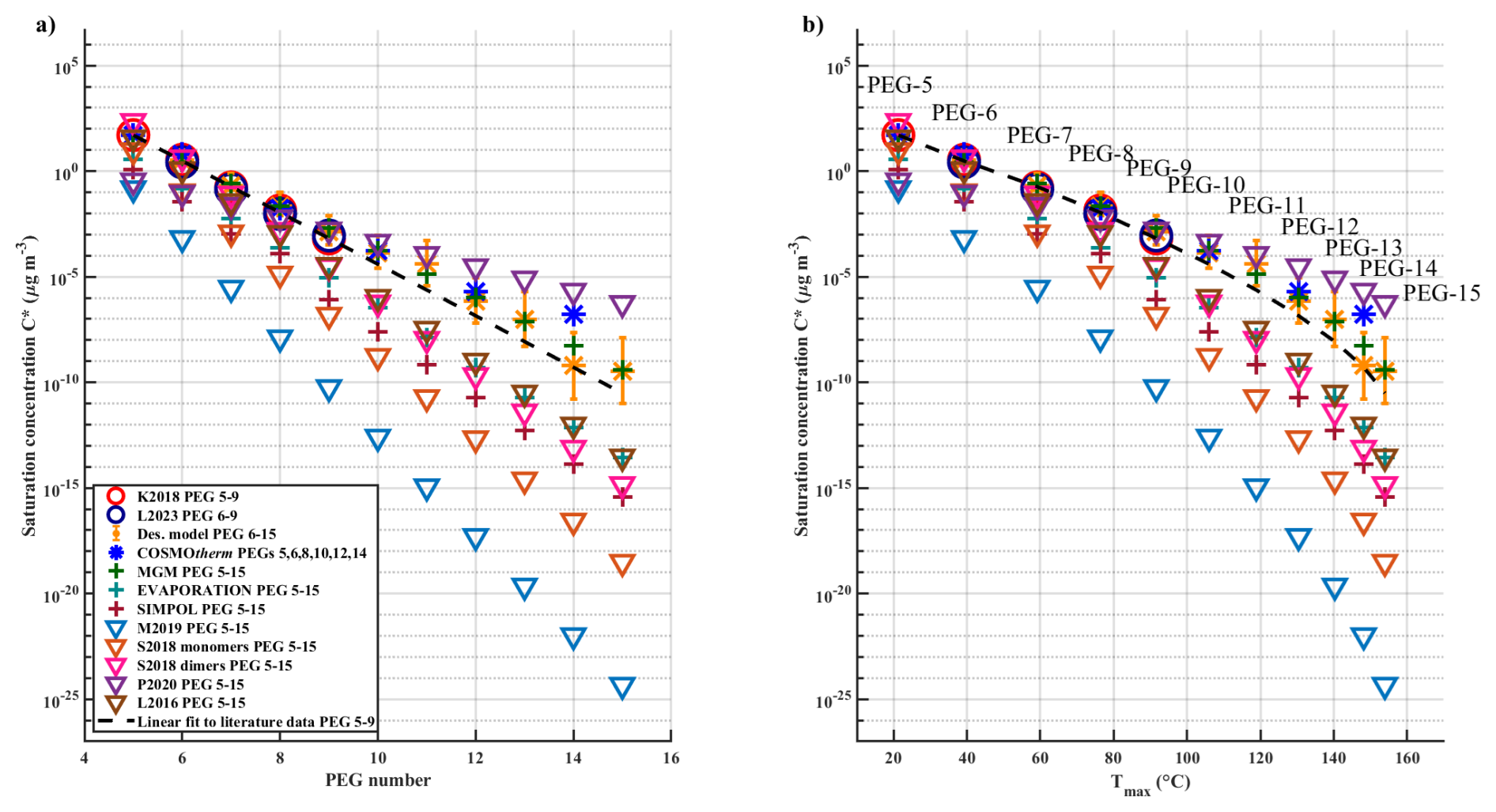
Figure 1 (a) PEG number vs. C^* estimated with different methods, as explained in the text. Circles show measurements-based values from literature (K2018 = Krieger et al., 2018; L2023 = Li et al., 2023). Yellow stars are desorption model results with whiskers indicating uncertainties; blue stars are COSMOtherm model results. Plus signs show parameterizations based on molecular structure; triangles show parameterizations based on molecular formula (L2016 = Li et al., 2016; S2018 = Stolzenburg et al., 2018; M2019 = Mohr et al., 2019; P2020 = Peräkylä et al., 2020). The dashed line is a linear fit to average values of PEG 5-9 from K2018 and L2023. (b) Measured average T_max values from all experiments vs. C^* determined with different methods (the same legend applies to both panels).

Almost all used models estimate a broadly log-linear decrease in volatility (C^*) when compared against PEG-number (Fig. 1a), except for COSMOtherm, MGM and to some degree the desorption model, which both estimate higher volatilities than just linear extrapolation from literature data. Note that although many models appear to estimate loglinear decrease in volatility vs. PEG-number (and thus molecular mass), true linearity should not be expected, as has been pointed out in previous studies (Li et al., 2016; Mohr et al., 2019; Stolzenburg et al., 2018). When comparing the estimated C^* results to measured T_max (Fig. 1b), the relationships appear only log-linear for the smaller PEGs but turn out roughly log-polynomial over the full range of PEGs 5-15. This effect is further discussed in the next section.

3.2 Impact of non-linear FIGAERO calibration

Note that previous investigations of C^* using FIGAERO data have typically assumed a log-linear relationship with measured T_max. To illustrate the impact of the log-polynomial relationship of C^* vs. T_max found here (Fig. 1b), we applied the original log-linear calibration, Eq. (1), to C^* vs. T_max data for PEGs 6-9 and two modifications that follow a second-order polynomial

$$\begin{array}{}\text{(12)}& \ln \left(P_{\mathrm{sat},\mathrm{meas}}\right)=a{T}_{\max ,\mathrm{meas}}^{\mathrm{2}}+b{T}_{\max ,\mathrm{meas}}+c\end{array}$$

and a third-order polynomial

$$\begin{array}{}\text{(13)}& \ln \left(P_{\mathrm{sat},\mathrm{meas}}\right)=a{T}_{\max ,\mathrm{meas}}^{\mathrm{3}}+b{T}_{\max ,\mathrm{meas}}^{\mathrm{2}}+c{T}_{\max ,\mathrm{meas}}+d,\end{array}$$

where a, b, c and d are free parameters that we fit to C^* vs. T_max data for PEGs 6-15. (PEG-5 was omitted as only a decaying signal of it was observed, so its T_max is uncertain; the value for PEG-15 is based on extrapolation as described in Sect. 3.3.) In the absence of literature P_sat (or C^*) values for PEGs 10-15, we chose the results from desorption modelling to be the best estimation of C^* values for these compounds and used those results as the basis for the fit. This choice is further discussed in Sect. 3.3. The performance of all models in estimating C^* is also further discussed in Sect. 4. The bivariate least squares fit algorithm used for linear fitting (see Sect. 2.2.1) is not suitable for polynomials. Therefore, we employed the Gauss–Markov original least squares regression in those calculations. This method takes into account the uncertainties in the y axis (P_sat,meas) but not the uncertainties in the x axis (T_max). Note that using different fitting methods that do or do not take all uncertainties into account can cause the fit to unduly weight some points more than others, and care should be taken when selecting an appropriate fitting routine. Besides Gauss–Markov estimation, Weighted Least Squares regression, Orthogonal Distance Regression or Bayesian regression can be used for fitting polynomials with uncertainties.

Figure 2a shows how different polynomial fits match the C^* vs. T_max values fitted to desorption model results, namely a linear fit, a 2nd order polynomial and a 3rd order polynomial. We then investigated how these different fit equations affect the VBS (Volatility Basis Set, Donahue et al., 2011) distribution of sesquiterpene SOA determined with FIGAERO-CIMS. Details about the sesquiterpene SOA production and FIGAERO measurement can be found from Ylisirniö et al. (2020). We highlight that this relatively older dataset is used here merely for illustrative purposes. Accurate FIGAERO volatility calibrations should always be conducted using the same instrumentation as in the actual ambient or laboratory experiments, using the same setup and settings (ideally at a similar time, to avoid drifts) and even similar aerosol particle sizes and filter loadings.

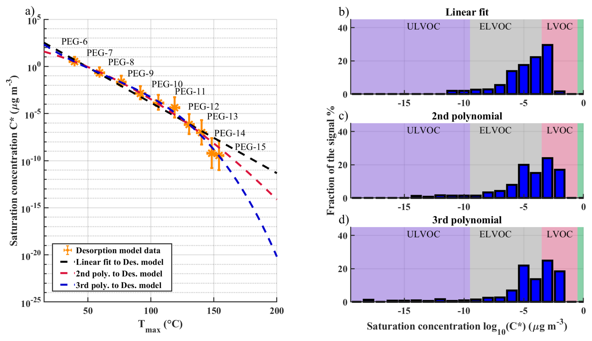
Figure 2 Panel (a) shows different log-linear and log-polynomial fits to C^* vs. T_max values, with C^* values determined with desorption modelling. Panels (b), (c) and (d) show VBS distributions determined from FIGAERO – CIMS measurement of sesquiterpene SOA, determined with different fit equations. LVOC, ELVOC and ULVOC refer to the categories of low-volatility, extremely low-volatility and ultra-low-volatility organic compounds, respectively, which are defined by respective ranges of volatility as indicated by the background color shades (red, gray, purple; Schervish and Donahue, 2020).

When inspecting Fig. 2a more closely, we can notice that different fit equations agree well with each other up to about PEG-12 (log 10(C^*) ∼ −6 µg m⁻³), after which the second and third-order polynomial fits increasingly differ from the linear fit. The second and third-order polynomial fits agree with each other and measured values within an order of magnitude up to PEG-14 (log 10(C^*) ∼ −10 µg m⁻³), after which the third-order polynomial fits the desorption model data better. When comparing the resulting VBS distributions of the three fits (Fig. 2b–d), we can see that the main differences in the three distributions are in the region of ultra-low-volatility organic compounds (ULVOC, log 10(C^*) < −9 µg m⁻³) (Schervish and Donahue, 2020). These divergences illustrate how the availability of calibrants up to higher T_max substantially improves the volatility calibration for FIGAERO, including any extrapolation to even higher T_max, which is also subject to the choice of fitting function. Higher accuracies, especially for ULVOCs, may still be achieved by extending calibration measurements further up to, e.g., PEG-18 or PEG-19, to cover an even wider T_max range. It is also likely that some other fit equation could yield more accurate results than our polynomial fits. However, taking into account current uncertainties in determining the volatilities of low-volatility calibrants, including our results in this study, simple polynomial fits seem to provide adequate approximations within the range of T_max measurements.

3.3 Desorption modelling results and uncertainties

The analysis in Sect. 3.2 relied not only on the measured T_max but also on the estimated P_sat (C^*) of PEGs > 9, for which literature values have not yet been established. To justify our selection of C^* values from the desorption modelling, we present here a more detailed description of how the model runs were set up, how model parameters were fit to the measured FIGAERO-CIMS data, and how we evaluated our results. In Fig. 3, we present the thermograms measured with FIGAERO-CIMS in one of the experiments. The thermograms peaked (T_max) between 37 °C (PEG-6) and 150 °C (PEG-15). PEG-5 proved to be so volatile that only a decaying signal was observed. In a colder environment, its T_max would likely be just prior to the start of the temperature ramp at room temperature, at ∼ 18 °C. The figure also shows a desorption model fitting result, fitted to the measurement data by choosing suitable values for the saturation vapour pressures (P_sat, i) and vaporization enthalpies (ΔH_i) for each compound (i) at 298 K, along with instrument sensitivities S_i (Sect. 2.3.1). Model fits could be achieved equally well either while assuming constant ΔH_i values, or while assuming a small temperature dependence due to the expected change in heat capacity upon vaporization. Here, we used a temperature dependence of $d\mathrm{\Delta }H/\mathrm{d}T$ = −0.1 kJ mol⁻¹ K⁻¹ as a rough literature-based estimate (Krieger et al., 2018), but which is similar to dependences found also for a broader range of organic compounds (Bilde et al., 2015; Epstein et al., 2010; Riipinen et al., 2007; Tong et al., 2004). Note that the model fits the thermogram upslopes very well, suggesting an accurate representation of the desorption process. Also, the downslopes, which arise primarily from post-desorption transport processes, are fit well overall, though they are simulated using the same heuristic approach and the same parametrization as originally estimated rather crudely (Schobesberger et al., 2018).

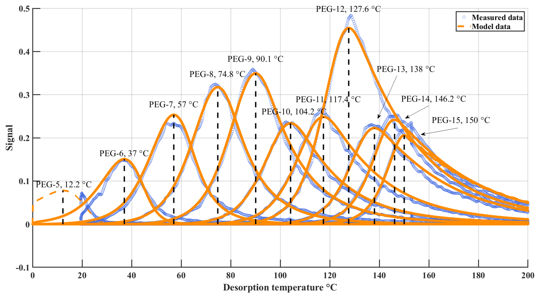
Figure 3 Thermograms measured by FIGAERO-CIMS in “experiment A” (see text for details) for monodisperse aerosol consisting of PEGs 5-15 (blue) and example results from desorption modelling (orange) after fitting model inputs for P_sat, i, ΔH_i, and S_i for each PEG (i = 5…15; see Sects. 2.3.1 and 3.3).

The automated optimization of the model parameters (applied 24 times for each experiment) followed the covariance matrix adaptation evolutionary strategy (Hansen and Ostermeier, 2001); the quality of each fit (f) was defined for each PEG as the mean square deviation between model and measurement, considering data up to just after (40 s) the peak of the thermogram, as subsequent data were increasingly subject to non-idealities that the model captures with varying success (tails; e.g., Fig. 3). We only selected experiments with filter loadings of < 200 ng, to minimize potential biases due to matrix effects, which can delay desorption (Huang et al., 2018; Ylisirniö et al., 2021) but are not part of the model (which always assumes well-separated individual particles).

The experiments were made in January (A, B) and July (C) of 2022; they used filter loadings of 105 (A, B) or 170 (C) ng, collected over 0.3 (A, B) or 4 (C) min, and desorption temperature ramp rates of 0.22 (A), 0.69 (B) or 0.32 (C) K s⁻¹, which correspond to heat ramping times of (A) 15 min, (B) 5 min and (C) 10 min. Experiment A was part of a series testing for filter loading effects (105, 205, 1100 ng) that showed increasingly delayed desorption with increasing loading, as expected; this effect was notable already when doubling the loading to 205 ng. The 105 ng experiment also exhibited the least tailing in its thermograms (of all considered experiments). In conclusion, experiment A appeared to be the least affected by non-idealities of all experiments; it also routinely yielded the lowest (best) values for f. We thus also show model-fitting results from experiment A separately in Figs. S1 and S2 in the Supplement. For our best estimates for P_sat, i, ΔH_i and their uncertainties (Figs. 1, 2, S1, S2; Tables S1–S3), we first determined best estimates for each experiment individually ($\mathrm{1}/f$-weighted means of all successful optimizations, defined as those within 10 % of f^*, the lowest f obtained by the 24 optimizations), followed by the $\mathrm{1}/f^{*}$-weighted mean (experiment A double-weighted) over all experiments. For P_sat, i, these calculations were performed in logarithmic space.

Starting the temperature ramp at a lower temperature in the model, such as 0 °C, a thermogram can also be simulated for PEG-5 (Fig. 3, dashed line), but P_sat, i and ΔH_i could not reasonably be constrained by our optimization routine and are thus not reported for PEG-5. Also, PEG-6 is already observed desorbing from the very beginning of the experiment, substantially altering the thermogram's upslope and thus preventing us from obtaining as reliable model optimizations for ΔH as for larger PEGs. But as its desorption occurs near room temperature, P_sat was nonetheless well constrained, so we report P_sat for PEG-6 but not ΔH.

At the other end of the scale, the automated model optimization did not work well for PEG-15. In order to reduce computational expense, the algorithm optimized pairs of P_sat, i and ΔH_i for each PEG-i separately while the desorption of the sum of all other PEGs was approximated to provide appropriate condensed-phase mass fractions of the PEG-i, as that fraction affects evaporation rates (Raoult effect). Comparisons with results of (slower) model runs that properly simulated the desorption of all PEGs simultaneously showed negligible differences for all but the last-desorbing species, PEG-15. Therefore, the reported desorption model values for PEG-15 (Figs. 1–2; Tables S2–S4) are not result from optimization but a log-linear extrapolation of the results for PEGs 6-14.

Besides the success of the desorption model in fitting the FIGAERO-CIMS measurements, the resulting values of ΔH_i and even more so P_sat, i are also in excellent quantitative agreement with previous experimental findings for PEGs 5-9 (Krieger et al., 2018; Li et al., 2023) (Figs. 1, S1, S2; Tables S2, S4). Further, more heuristic confidence in our model results is created by their agreement with the MGM (Fig. 1). It is also interesting to note that our results for higher-order PEGs broadly continue the linear trend of ΔH_i and the log-linear trend of P_sat, i vs. PEG order (or mass) that previous studies reported for PEGs 5-9 (Figs. S1–S2; especially experiment A). However, our uncertainties do increase for higher-order PEGs, and in principle, log-linearity should not be expected. Indeed, both COSMOtherm and MGM predict a slight departure from that log-linearity with increasing PEG order, consistent also with the desorption model results and their uncertainties (see also Sect. 3.1 and Conclusions).

4 Discussion

4.1 Measurement accuracy and performance of the desorption model

In the previous section, we argued that the desorption model produces among our best estimates of P_sat (C^*) for PEGs, at least for PEGs 6-14, mainly motivated by the high accuracy with which the model can replicate the overall behaviour of the measured thermograms. We obtained uncertainty estimates for individual experiments by assessing the sensitivity of fit quality to variations in P_sat, i and ΔH_i. But ultimately, the main source of uncertainty for the desorption modelling results stems from variabilities in our FIGAERO-CIMS measurement results. We know that several experimental details affect the thermograms, in particular the values of T_max; most prominently the desorption temperature ramp rate, the size of deposited aerosol particles and total filter mass loading (all of which work to increase T_max). The effects of ramp rate and particle size are well understood and accountable in the model (Thornton et al., 2020; Ylisirniö et al., 2021), and filter mass loading effects should be negligible at low-enough loadings, at which we expect individual deposited particles to be well separated. However, even when accounting for those effects and only considering loadings of < 200 ng, we encountered variabilities in T_max values and in thermogram shapes (especially tails) that we have not been able to explain. The desorption model nonetheless achieved subjectively good fits of the thermograms (except for tails, when they were elevated compared to experiment A), and the variabilities between experiments translated to variabilities in the obtained values for P_sat, i and ΔH_i that are the main source of reported model uncertainties.

We hypothesize that the following three potential issues can be involved in producing variabilities between measurements, though we have not endeavoured to elucidate their respective roles or effects quantitatively:

• 1.

  The heating of the IMR was found to generally reduced thermogram tailing. A custom-built heating system was used in our experiments (see Sect. 2.2) aiming for a uniform IMR heating.

• 2.

  We found that allowing a longer time for the PEG aerosol to “dry” (i.e., evaporate remaining solvent; Sect. 2.1) sometimes led to a reduction of T_max. We hypothesize that the deposition of not fully dried PEG aerosol facilitates matrix effects on the filter. Consequently, we have paid attention to ensure sufficient “drying” of the PEG aerosol for our calibration experiments. Impacts of retained solvents in P_sat measurements have been reported and discussed in earlier studies, e.g., finding an effect in the opposite direction for carboxylic acids (e.g., Bilde et al., 2015; Cappa et al., 2007, 2008).

• 3.

  The FIGAERO typically utilizes a k-type thermocouple for temperature measurement, which typically has a measurement error of ± 2.2 K. Additional ∼ 1 K of reading error can be also introduced by the electronics of the measurement system. However, k-type thermocouples are also sensitive to reading errors caused by static electric fields that can sometimes form to the PTFE surfaces of the FIGAERO inlet. This could possibly be improved by using a different kind of thermometer such as PT100 or PT1000 temperature probe, although this might require some redesigning of the inlet system. There may also be some variability in the exact position of the temperature probe, and the desorption flow of nitrogen may have a significant temperature profile, both radially and in the direction of the flow.

Acknowledging all these sources for uncertainty, we estimate that our reported values from the desorption modelling are still roughly within up to 2 orders of magnitude of the “true” values; especially for larger PEGs, whereas the estimates for smaller PEGs are better constrained (Figs. 1, S1, S2). However, that level of uncertainty makes our estimates still accurate enough for most applications, considering the vast scale of different C^* values spanned (Fig. 1; spanning nearly 20 orders of magnitude) and the similarly wide scales typically relevant in studies of SOA.

4.2 Parametrizations of molecular formulas

Comparing the output of molecular formula parametrization-based models (L2016, S2018, M2019, P2020) to results from the desorption model as well as literature for PEGs 5-9, most parametrization models tend to underestimate the C^* value of PEGs, especially at the higher-order polymers (the exception being P2020). The biggest discrepancies result from M2019 and the two variants of S2018, most likely stemming from the fact that these models have been trained on relatively specific datasets, focusing on α-pinene-derived HOMs. In those HOMs, oxygen atoms are often found in carboxyl, hydroxyl, and hydroperoxyl groups, which substantially reduce the compounds' saturation vapor pressures. But for PEGs, the larger they are, the more of their oxygen is found in ether groups, which are relatively less “efficient” in reducing a compound's vapor pressure. Thus, M2019 and S2018 are simply the least fit for predicting the vapor pressures (C^* values) of PEGs. The L2016 parametrization, on the other hand, performs better, maybe due to being based on a more balanced training set of organic compounds. It performs particularly well for the smaller PEGs (for which C^* are also better established), in line with the increasingly unusual dominance of ether groups in the composition of larger PEGs.

P2020 compares quite differently to the results from literature and our desorption model: underestimating C^* (by up to 2 orders of magnitude) for lower-order PEGs but then overestimating (by up to 3 orders of magnitude) for higher-order PEGs. It was trained on α-pinene-derived HOMs, much like M2019 and S2018, but using a fundamentally different approach than all other parametrizations considered in this study. Also, for typical HOM formulas, notable discrepancies result; e.g., C₁₀H₁₄O₉ yields a C^* of 0.33 µg m⁻³ via Eq. (11) (P2020) but only 6.3 × 10⁻⁴ µg m⁻³ via Eq. (10) (M2019). Therefore, the overall differences in the results obtained by these parametrizations also reflect our still poor understanding of the volatility of HOMs (such as from α-pinene oxidation). The discrepancies between the parametrizations are amplified here by applying them to PEGs, and increasingly so for larger PEGs.

4.3 Group contribution methods (MGM, SIMPOL, EVAPORATION)

Overall, the group contribution methods appear as somewhat more accurate predictors of saturation vapor pressures than the simpler formula-based parametrizations (Fig. 1a) – as may be expected from their more complex approach that involves molecular structural information. Nonetheless, both SIMPOL and EVAPORATION results increasingly deviate from our experiment-based estimates with increasing PEG order (qualitatively similar to most formula-based parametrizations): up to ∼ 5 orders of magnitude for SIMPOL, and up to ∼ 3 orders of magnitude for the more elaborate EVAPORATION model. Specifically, they seem to overestimate how much each additional ether group reduces the vapor pressure.

The MGM model, on the other hand, seems to perform very well in estimating C^* values of PEGs, with only relatively small deviations, generally within an order of magnitude, from both previous experimental results (K2018, L2023; PEGs 5-9) and the results we found here via fitting the desorption model to our experiments (PEGs 5-15). Thereby, the MGM notably outperforms both SIMPOL and EVAPORATION, even though those provide direct predictions of vapor pressures, whereas the MGM first predicts boiling points, from which the vapor pressures are only subsequently calculated. It is beyond the scope of this study to explore what may be the reasons behind the relative success of the MGM. But we hypothesize that the MGM could be more robust, because it is based on a much larger set of compounds, for which boiling points have been measured: 4426 organic compounds, whereas SIMPOL and EVAPORATION are based on saturation vapor pressure measurements for 272 and 579 organics, respectively. Especially the larger PEGs consist mostly of multiple ether groups, which is relatively uncommon and less likely to be sufficiently represented in the smaller training sets.

4.4 COSMOtherm

COSMOtherm is by far the most complex model used in this study to determine C^* values of the PEG's. The results from COSMOtherm are in good agreement with literature values and desorption model results for the C^* of PEGs 5-10 and only significantly deviate from the desorption model for PEG 14, the largest PEG calculated using COSMOtherm. The computational cost of the COSMOtherm calculations increases dramatically with increasing molecular size; PEG-14 is a large molecule in light of all discussions in this study, with a chemical formula of C₂₈H₅₈O₁₅ and no branching. Consequently, the COSMOtherm calculations for PEG-14 were those with the highest level of simplification (i.e., in number of conformers searched), and it is here where we would first expect errors. Note that our application of COSMOtherm was an iterative process that took into account the agreement of intermediate results obtained for the smaller PEGs with the corresponding, previously published saturation vapor pressure values (K2018) (see Sect. 2.3.2). Overall, our results suggest that our approach with COSMOtherm was suitable for predicting C^* values for this homologous series up to compounds with at least 4 orders of magnitude lower C^* (PEG-12) than the lowest previously known C^* (PEG-8).

5 Summary and conclusions

In this study, we set out to determine estimates of P_sat (C^*) values for PEGs 5-15 using a variety of different estimation methods. In the same process, we also compared how different saturation vapor pressure estimation methods differed from each other. We found that the different methods can produce up to 18 orders of magnitude differences in estimated C^* values (Fig. 1a, PEG-15). We argue that we achieve the best estimates for the volatilities of the PEGs (at least for PEGs 6-14) by fitting an explicit aerosol desorption model to our thermal desorption-based FIGAERO-CIMS measurements of PEG aerosol. These estimates are in excellent agreement with previous findings on the volatility for PEGs up to PEG-9. Our uncertainty ranges for C^* increase to up to 3 orders of magnitude for the largest PEGs, mainly due to variabilities between sets of experiments. Within an order of magnitude, however, our best estimates continue a broadly log-linear dependence of P_sat (C^*) on PEG order (or mass) up to PEG-14, in agreement with literature on PEGs 5-9. Analogously, the dependence of ΔH on PEG order broadly continues its linear trend as well (Fig. S2).

We also explored a variety of theoretical and (semi-)empirical methods that are commonly used in the field to estimate saturation vapor pressures for organic compounds, absent measurements: from quantum chemistry-based calculations to molecular structure-based group contribution methods, to simple parametrizations based on molecular sum formulas. Generally, the simpler the method and the larger the considered PEG compound, the larger the errors, as the variety of estimates of C^* spanned up to 18 orders of magnitude. These results demonstrate that any of the formula-based parametrizations need to be used with caution, keeping in mind especially how a specific parametrization was developed. Most parametrizations we considered were specifically developed for α-pinene-derived HOMs, using relatively small sets of representative compounds. However, our understanding of the often-complex structures of these HOMs and of their inter- as well as intra-molecular interactions has been subject of recent and current research. Consequently, the respective parametrizations can be useful in pertinent studies, but their application to compounds of generally different compositions will likely be problematic, as seen here for PEGs. Another considered parametrization, developed for a broader, more diverse set of organics, achieved better accuracy overall, though it still typically underestimated C^* by orders of magnitude. Similar estimations as by that broader parametrization were obtained by two common group contribution methods (SIMPOL, EVAPORATION), whereas those obtained by a third method (MGM) broadly agreed with our best estimates. Although the MGM obtains C^* values less directly, we suggest that the method could be a robust alternative nonetheless, possibly thanks to being based on a wider set of organics than SIMPOL and EVAPORATION. In many practical applications, however, a downside of all group contribution methods is that the target compounds need to be identified at the level of their molecular structures before the models can be utilized, which is typically not achieved by state-of-the-art mass spectrometry-based measurements of oxygenated organic compounds in the atmosphere. The same limitations apply to using COSMOtherm for estimating volatilities, and it also requires increasing levels of simplification or higher computational resources when considering larger molecules. Our COSMOtherm application did, however, yield promising results. In conclusion, we suggest that measurements of the thermal desorption behaviour of aerosol constituents can be a more versatile and reliable way of determining their volatility. Useful quantification of that volatility will not necessarily require (possibly complex) model simulations, like in this study, but can achieve sufficiently accurate (within an order of magnitude) results by reference to the desorption behaviour of calibration compounds with known volatilities, such as aerosol particles consisting of a mixture of PEGs.

Notably, a closer look at Fig. 1a (and Fig. S1) suggests that toward the larger PEGs, there may be a slight deviation toward higher C^* values compared to the log-linear extrapolation from PEGs 5-8, which is also in line with the independent COSMOtherm and MGM model results. On the other hand, the nominally “best” desorption model fits suggest the log-linear extrapolation may be an excellent predictor up to PEG-14. More precise sets of measurements are needed to elucidate the volatility trends of those larger PEGs with better certainty. E.g., the desorption temperature measurement in the FIGAERO could be improved, and other aspects affecting reproducibility optimized (see Sect. 4.1). Also, the determination of ΔH and P_sat values via desorption modelling could be optimized to achieve quicker convergence and more robust uncertainty estimates, for example, by incorporating Bayesian estimation approaches.

Uncertainty also remains in what is the appropriate formal relationship between the logarithm of C^* and T_max (Figs. 1b, 2a). Unlike previous assumptions or hypotheses (Bannan et al., 2019; Lopez-Hilfiker et al., 2014; Mohr et al., 2017; Ylisirniö et al., 2021), it is not linear. It appears that a 2nd or 3rd-order polynomial relationship is instead suitable. Using previously published FIGAERO measurements of SOA, we explored the consequences of using such polynomial fits to calibration results up to ∼ 150 °C instead of a linear fit to calibrations only up to 90 °C. As demonstrated in Fig. 2, a calibration curve that is accurate up to higher temperatures is needed to accurately determine the volatility of compounds in the ELVOC and ULVOC ranges. Those compounds play a particularly important role, for example, in the climatically critical processes of atmospheric new particle formation and nanoparticle growth (Schervish and Donahue, 2020; Simon et al., 2020). Especially nanoparticle growth models rely on an accurate representation of the volatilities of the compounds involved (Stolzenburg et al., 2018; Tröstl et al., 2016).

An additional error source for practical applications of a T_max–C^*-relationship established via PEGs is likely due to the relatively low ΔH values we find for PEGs (in agreement with Krieger et al., 2018), when compared to broader sets of organic compounds (Fig. S2). As illustrated in Fig. S3, this discrepancy may induce overestimations for C^* assigned based on T_max measured for more typical organics but using a T_max–C^* relationship established for PEGs. As ΔH is of increasing importance with increasing desorption temperature, the expected average bias increases with decreasing C^*, up to about an order of magnitude in the ELVOC and ULVOC ranges.

To conclude, the most valuable contribution of this work is probably the determination of the volatilities (or, in more accurate terms, the saturation vapor pressures) of higher-order PEGs. Previous P_sat measurements were obtained up to PEG 9, which falls within the LVOC range, but the higher-order PEGs extend throughout the LVOC and the whole ELVOC ranges (Fig. 2). Our study thus provides knowledge for calibrating thermal desorption-based techniques for volatility measurements down to the transition to ULVOCs, while remaining uncertainties are likely acceptable for most applications. It is worth stressing that we expect that the knowledge of PEG vapor pressures will be useful beyond FIGAERO-CIMS measurements, i.e., for thermal desorption-based techniques more broadly, including some notable recent developments. For instance, a recently developed volatilization inlet (VIA, Häkkinen et al., 2023) provides truly online thermal desorption of aerosol particles, and when coupled to a nitrate CIMS, it has been demonstrated to detect and separate α-pinene-derived HOMs by their volatility, as well as PEGs (Zhao et al., 2024). There, the separation by volatility was only qualitative. But using this study's C^* values, the thermal desorption measurements for PEGs could serve as a calibration to quantitatively determine the C^* values of the detected HOMs, and of course also of other measured organics, down to extremely low volatilities. A similar new method for measuring particle volatility online that will most likely benefit from this work is the Wall-Free Particle Evaporator (WALL-E, Gao et al., 2025), which strives to minimize the thermal decomposition and vapor wall losses often observed with thermal desorption methods.