Laboratory and field characterization of an atmospheric pressure transverse chemical ionization ion-molecule reaction region

We introduce a custom-built, field-deployable, atmospheric pressure Ion-Molecule reaction Region (IMR) for use with Chemical Ionization Mass Spectrometry (CIMS), the so-called “t-IMR”. The design is described in quantitative detail and shows significant mitigation in potential measurement interference compared to other IMR configurations, particularly those operating at low pressure. The relatively large laminar flow and inner chamber diameter reduce the probability of sampled air and ion clusters interacting with the Teflon surfaces of the IMR before being detected by Time-of-Flight (ToF) mass spectrometry. This also leads to a substantial reduction in wall effects and artificial background signals for even low volatility organic products, as demonstrated in alpha-pinene ozonolysis experiments. An electric field is induced perpendicular to flow in the t-IMR to accelerate ions and consequent charged sample clusters to the MS interface. The strength of this field is modulated and optimized to simultaneously maximize total ion flux and instrument sensitivity. A sheath flow apparatus is introduced to provide small N₂ flows counter to ion and sample cluster flow into the MS to reduce the likelihood of particulate buildup and clogs to the pinhole separating the IMR from the MS, ensuring uninterrupted sampling for extended periods of time. Finally, we demonstrate the capability of the t-IMR to be deployed to the field to measure down to sub-ppt level ambient concentrations of important trace gases including reactive bromine at a ground-based site in the marine boundary layer. We find that the t-IMR design considerably reduces artificial signals from surface contact and wall effects, and improves detection of very low concentration species in the ambient atmosphere, with respective limits of detection of 0.06, 0.05, and 2 ppt for Br₂, HOBr, and HNO₃. The relationship between instrument sensitivity and IMR water vapor concentrations is also explored and applied to in-field measurements.

1 Introduction

Multiple trace gas species present in the atmosphere at concentrations on the order of parts per trillion (ppt) and below are known to have relatively large impacts on atmospheric composition, the climate system, air quality, and human health. Chemical Ionization Mass Spectrometry (CIMS) has allowed for online and in situ measurements of many such trace gases with high temporal resolution and molecular specificity when coupled to a time-of-flight or orbitrap mass spectrometer having sufficient resolving power and mass accuracy (Du et al., 2022). Chemical ionization has the advantage of preserving the integrity of the molecules being sampled. The softer the ionization process, i.e. the lower the net energy imparted to the analyte upon ionization, the less interference to analyte identification and quantification from chemical or physical processes during sampling. Adduct ionization, where a specific ion such as iodide (I⁻, used in all studies herein), nitrate, ammonium, CF3O−, etc, is used to form an ion-molecule cluster, has been shown to be especially soft compared to charge (proton) transfer, direct photoionization, or electron impact (Lee et al., 2014; Andrade et al., 2008). A key component of CIMS instruments is the Ion-Molecule reaction Region (IMR), where neutral analyte molecules obtain a charge (positive or negative) via charge transfer, reactive charge transfer, or ion-neutral adduct formation. The resulting analyte ions or clusters can then be guided by electric fields and fluid dynamics inside the mass spectrometer (MS).

The IMR design significantly impacts the sensitivity and selectivity of a CIMS to certain classes of compounds, background signals, and/or total ion flux all determine the limits of detection (LOD) at which atmospheric components may be measured (Robinson et al., 2022; Liu et al., 2019; Lopez-Hilfiker et al., 2016; Slusher et al., 2004; Huey et al., 1995). Many previous IMR designs involving the I⁻ reagent ion utilize a low pressure chamber (< 0.1 atm). The low pressure has practical and analytical benefits, such as allowing larger apertures for ions to enter the MS, reduced ion-molecule interaction times to minimize secondary ion chemistry without needing electric fields or high flows, and lower absolute water vapor concentrations, as humidity-dependent sensitivities have been reported for multiple compounds across CIMS measurements (Krechmer et al., 2018; Zhao et al., 2017; Kercher et al., 2009; Dörich et al., 2021). However, reducing the pressure of the IMR dilutes sample molecular number concentration by up to several orders of magnitude (Rissanen et al., 2019). This leads to a lower collision frequency between analytes and reagent ions for a given reaction time and thus lower ultimate sensitivity. In a low pressure IMR, it has been shown that even a relatively small increase in operating pressure can increase sensitivity (Novak et al., 2020). For species present at very low concentrations, these issues could prevent in-situ measurements of sub-ppt level compounds (Jokinen et al., 2012). Moreover, the expansion upon sampling through an orifice from approximately 1 to < 0.1 atm coupled with physical constraints to keep interaction timescales short, leads to turbulent mixing and enhanced wall interactions.

When considering IMR design, the two main objectives we consider include both generating a sufficient and stable stream of reagent ions to produce signal for analyte species and, of equal importance, the verification that measured signals are a true representation of the gases sampled, ambient or otherwise. This involves disturbing the sample gas as little as possible before it enters the CIMS. Multiple challenges arise in the pursuit of achieving this goal while maintaining a sufficient number of ion collisions for continuous measurement. One such problem is chemical reactions occurring in and on the surfaces of the IMR, which would alter the molecules before detection, thereby creating an artificial chemical signal not present in the actual atmosphere being sampled. One way to reduce this effect is to move the sample through the IMR as quickly as possible to reduce the likelihood of interaction with other molecules and/or surfaces, while ensuring sufficient ion intrusion. The residence time, or average time that an air mass spends in the IMR chamber before entering the CIMS, is controlled mostly by the pumping speed from an external air pump. Another consideration beyond flow speed is turbulent mixing, which is dependent on the pumping scheme and angle at which air enters the CIMS. Turbulence can decrease the likelihood of ion collisions and interfere with total detected signal, if not eliminate signals completely. Designing an IMR such that the inlet flows are as laminar as possible helps to eliminate small eddy formations and turbulence which increase molecular interactions and disturb reagent flows (Yang et al., 2024). There are also so-called IMR “wall effects”, which refer to a situation where ambient molecules are deposited onto or absorbed into the surface of the IMR to potentially be evaporated and reintroduced into sample flow at a later time. This not only causes an artificial depletion in a signal at the time of sampling, but also can create an enhancement in detection of that particular compound later, both of which misinterpret current ambient conditions and interfere with precise time of day measurements required to understand trace gas chemistry (Lopez-Hilfiker et al., 2014). Advancements in IMR design have been researched in pursuit of rectifying this commonly observed effect (Palm et al., 2019; Crounse et al., 2006). Choice of IMR surface material and experimental verification of wall effects are thus crucial to the reliability of resultant chemical signals.

This work introduces and demonstrates the capabilities of a field-deployable atmospheric-pressure “transverse IMR” using iodide reagent ions generated using a vacuum ultraviolet (VUV) lamp. This updated design is based off of a previous transverse IMR setup from Zhao et al. (2017) constructed with the intent of minimizing these common problems including turbulent mixing and wall interactions which lead to artificial and/or depleted CIMS signals. We describe in detail its design and evaluate performance based both on metrics determined in laboratory experiments as well as ambient measurements in the field.

2 t-IMR Description

We describe a Chemical Ionization inlet coupled to a Time of Flight Mass Spectrometer (i.e. a ToF-CIMS). We utilize a Tofwerk AG high resolution ToF-MS (model L-ToF). The design and operation of the ToF-MS and general coupling to chemical ionization regions has been described previously (Bertram et al., 2011; Lee et al., 2014; Lopez-Hilfiker et al., 2014; Riva et al., 2019). Briefly: analyte ions and remaining reagent ions are guided through a series of differentially pumped vacuum chambers, by segmented quadrupoles, one in the first stage downstream of the IMR with typical operating pressure of 2 mbar, and the other in the second pumping stage with pressures on the order of 10⁻³ mbar. Ions are then extracted into the ToF region (pressures typically on the order of 10⁻⁷ mbar) where they receive a pulse of energy and fly along a U-shaped path to a Micro Channel Plate (MCP) detector. In this process, the sample molecules are separated by mass due to differences in flight time. From these flight times, exact masses are calculated and binned resulting in the spectrum of ion counts versus mass-to-charge ratios for further analysis. For all data presented in this study, the default timescale of collected spectra is 1 Hz. Integration of peaks in each mass spectrum results in time series of all identified species, reported in default units of counts from the MCP in the ToF region. In order to convert detector counts to the relevant atmospheric concentration, a sensitivity value must be determined for every identified species (Lopez-Hilfiker et al., 2016). Sensitivities are typically quantified in units of counts ppt⁻¹ and are preferably determined by direct calibration, i.e. introducing a known concentration of a given species into the IMR and recording the corresponding instrument response for a set period of time such that the signal is stable and reproducible.

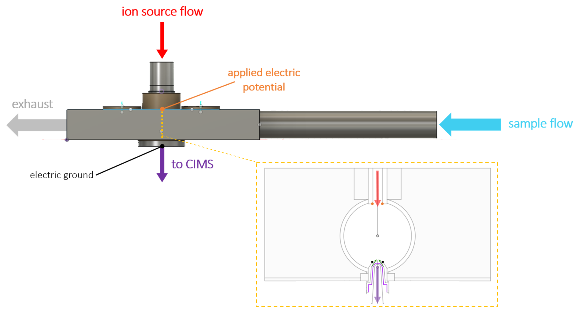
Figure 1 Schematic of the transverse IMR (t-IMR). A continuous 1 in. OD Teflon inlet held in place by stainless housing carries sample air at atmospheric pressure at a flow rate of 10 L min⁻¹ where it is then intersected at 90° by a 1.5 L min⁻¹ flow carrying the I⁻ reagent produced from a VUV ion source, which is accelerated by an electric potential toward the CIMS. The gold dashes in the housing schematic and corresponding inset show the location and a detailed cross section of the t-IMR. Reagent flow is again shown in red while sample + ion flow into the CIMS is shown in purple. For the inset the standard 10 L min⁻¹ flow through the t-IMR cavity (ID = $\mathrm{7}/\mathrm{8}$ in.) points out of the page. The critical orifice conical capillary is highlighted with purple outlining. The smaller sheath counter-flow is indicated with green arrows. Electric potential application is shown with orange points, with electric ground in black.

Shown in Fig. 1 is a schematic of our new transverse IMR, henceforth referred to as the “t-IMR”, where the inlet is comprised of a 1 in. (2.54 cm) outer-diameter (OD) PFA Teflon™ tube with $\mathrm{1}/\mathrm{16}$ in. (0.16 cm) wall thickness housed in an aluminum block, which is secured to the ToF-MS. The distance from the upstream edge of the 1 in. OD tube (i.e. the entrance to the IMR region) to the reagent intersection/MS ports at the center of the aluminum block housing is 32.4 cm, and the total length of the IMR tube is approximately 47 cm. The aluminum block is used mainly for stability, port alignment, and ability to be electrically grounded. Thus, when mentioning the t-IMR in this work, we are referring to the 1 in. OD teflon inlet tube acting as the ion-molecule reaction chamber, which is noted above as longer than the block housing it. This design brings ambient air into the ionization region continuously such that the sampled air flow does not experience any steps in diameter, corners, or other surfaces until it is exhausted beyond the aluminum block and capillary MS entrance area. The 1 in. OD Teflon tube extends upstream of the housing to ensure development of laminar flow and sampling outside of the overall instrument boundary layer. Figure 1 highlights the laminar sample flow of 10 L min⁻¹ (blue arrow) intersected by reagent ions (red arrow) which are accelerated by the induced electric field created by the applied potential between the ion source and the grounded capillary entrance to the ToF-MS, where newly formed analyte clusters enter the MS, indicated by the purple arrow. A transverse geometry is employed in this design to allow for larger (laminar) sample flow without concerns of turbulence or eddy formation at the MS entrance. This orientation is also meant to reduce contamination and dilution of the sample flow via neutral compounds in the outflow the ion source which experience no electric force from the applied potential. Such compounds in this case would likely be pulled by the large inlet flow to the exhaust before interacting with analytes sampled by the MS.

Iodide reagent ions are generated via a gaseous mixture of methyl iodide (CH₃I) and toluene (C₆H₅CH₃) carried by ultra-high purity nitrogen gas (UHP N₂ ≥ 99.999 %) at a combined standard flow rate of 1.502 liters per minute (L min⁻¹). Optimal flows for instrument operation were determined to be 1.5 L min⁻¹ through the CH₃I permeation tube channel and 2 standard cubic centimeters per minute (sccm) over the head space of a vial containing a volume of 2–3 mL of toluene. This gas mixture is then introduced into the cavity of an ionization device (a VUV lamp for all studies herein), ultimately producing I⁻ reagent ions introduced into the t-IMR at the point of the applied electric potential, indicated in orange in Fig. 1. A previous version of the atmospheric pressure, transverse IMR without the VUV ionization source is described in work by Lee et al. (2023) examining pinene oxidation.

Shown in the gold-bordered inset of Fig. 1 is a cross-sectional view of the t-IMR, where the sample flow direction points out of the page, reagent ion flow is shown in red, the sample + ion flow into the MS in purple, and electric potential application indicated with orange dots (with ground in black), analogous to the rest of the schematic. The critical orifice used to separate the IMR from the small segmented quadrupole (SSQ) region (the MS entrance) is a small cone that is 10 mm in length which extends approximately 2.5 mm into the t-IMR chamber, and has a pinhole with a diameter of 0.20 mm where air enters the capillary. The internal cavity downstream of the orifice is also conically shaped, with the diameter expanding to 3.7 mm toward the SSQ region from the pinhole interface. The orifice, highlighted in purple in the inset, is designed with a rigid pinhole sized to maintain the pressure difference between the IMR at ambient pressure on the order of ∼ 1000 mbar and the SSQ operating at 2 mbar. Low pressures in the BSQ and ToF chambers of the CIMS are maintained by a Pfeiffer Splitflow turbo pump, which in addition to the SSQ are back by an Ebara model EV-PA 500 pump. The Ebara pump is throttled with a manual valve to achieve a pressure of 2 mbar when the critical orifice is open to ambient pressure. Given the small size of this capillary separating the CIMS from the IMR, buildup and/or clogging due to particulates can be of concern depending on operating conditions. This is addressed via the addition of a sheath flow apparatus implemented to provide a small concentric flow of UHP nitrogen gas around the capillary, running opposite in direction to the flow being sampled through it into the MS (shown with green arrows in the inset). The standard flow rate used in environments with assumed relatively large particulate concentrations is 200 sccm, held steady (as are all other specific instrument flows) by a mass flow controller (MFC). This small counter-flow prevents a significant fraction of larger airborne particles from depositing onto the capillary which could lead to eventual blocking of the sample orifice. The sheath flow therefore allows for prolonged sampling periods (at least several days) uninterrupted by cleaning that would be otherwise necessary to clear blockages and prevent an interruption in the flow between the IMR and the SSQ chamber. Additionally, this sheath flow likely acts to partially dry the ion flow into the MS, leading to the evaporation of weakly bound water clusters formed when sampling high humidity air.

A diagram of the ionization setup used in all studies presented in this work, is shown in Fig. A1. Both the block and inlet tube contain ports for reagent ion flow generated with a VUV photo-ionization device (Jiang et al., 2023), as well as a port for the critical orifice or capillary entrance between the SSQ region of the CIMS and the atmosphere/t-IMR. Use of VUV to generate iodide ions for CIMS work has been demonstrated previously by Ji et al, who report similar instrument sensitivities, reagent ion production, and resultant mass spectra to those obtained with established radioactive sources (Ji et al., 2020). Our VUV ionizer setup uses a Heraeus PKS106 UV lamp held in custom stainless steel housing, the base of which is the cavity for ionization, including a female Swage fitting for $\mathrm{1}/\mathrm{8}$ in. OD tubing (reagent flow input for this study) along with a $\mathrm{1}/\mathrm{4}$ in. OD output tube (ion output) built in. The $\mathrm{1}/\mathrm{8}$ in. port acts as the entrance for both the reagent and carrier gases, which here are the CH₃I + toluene and UHP N₂, respectively. The lamp utilizes krypton gas to generate UV ionization light with a photon energy of 10.6 eV while requiring a DC voltage of 1.5 kV. Once in the lamp housing cavity, CH₃I is ionized by the UV radiation supplied by the lamp, aided by toluene acting as a photosensitizer.

The VUV setup produces an outflow of I⁻ ions carried in the UHP N₂ from the VUV housing into the t-IMR chamber. The use of the VUV marks a notable difference between this design and that of Zhao et al. (2017), as it does not require the use of salt solutions for ion production as the extractive electrospray ionization (EESI) method does, but rather uses a slow release permeation tube. This prolongs the potential continuous sampling of the t-IMR CIMS, as salt solutions need not be replenished for reagent production, while also avoiding potential clogging of capillary delivery tubes involved with EESI. Both theirs and our setups eliminate the need for radioactive sources used in many previous CIMS experiments, which can be difficult to deploy to remote field sites, as well as presenting a higher potential hazard level for operation. Though it is important to note that our VUV device may be replaced by any other ionization instrument (including a radioactive source if so desired) at the user's discretion.

One notable effect of the specific VUV orientation in this setup is the exposure of sample air to a small amount of UV radiation, which has the potential to change sample composition as well as create ${\mathrm{O}}_{\mathrm{2}}^{-}$ ions which can create unintended additional analyte ions. These ${\mathrm{O}}_{\mathrm{2}}^{-}$ cluster peaks may appear at similar mass-to-charge ratios ($m/Q$s) and potentially complicate the identification of certain compounds clustered with I⁻ in the negative mode for the CIMS. This has been reported by Ji et al. (2020) and is diagnosed in our setup mainly by the signal of the fitted compound ${\mathrm{CO}}_{\mathrm{3}}^{-}$ at $m/Q$ 60 in the mass spectrum. In all laboratory experiments presented here, it is found that the mean ${\mathrm{CO}}_{\mathrm{3}}^{-}$ signal is always less than 0.5 % of the reagent signal (${\mathrm{I}}^{-}+{\mathrm{IH}}_{\mathrm{2}}{\mathrm{O}}^{-}$), in many cases under 0.05 %, and does not interfere with the identification and quantification compounds of interest. This is due to the much higher signals for iodide clusters and importantly the mass defect of I⁻ (separated from ${\mathrm{O}}_{\mathrm{2}}^{-}$ clusters) easily identified with the high resolution LToF instrument. That said, it is recommended for generally cleaner spectra to reduce sample exposure to the VUV lamp, as done by Ji et al with a 90 degree bend in their reagent delivery line, which is a design element we will likely incorporate into future versions. High ${\mathrm{CO}}_{\mathrm{3}}^{-}$ signals are typically observed when air leaks are present in the UHP N₂ reagent delivery lines, as even a minuscule amount of air can lead to an O₂ concentration similar to that of CH₃I in the UV-illuminated volume, which would likely result in ${\mathrm{O}}_{\mathrm{2}}^{-}$ clusters present in spectra.

The t-IMR chamber is sealed against the ionizer and SSQ entrance via, press-fit O-rings and screws holding the block to the CIMS face, such that the t-IMR is only open to ambient air at its entrance and ultimately the external pump throttle to control the flow rate. The ionization and critical orifice ports are aligned for reagent flow to be perpendicular to and combine with sample flow. The standard flow rate chosen for operation of the t-IMR is 10 L min⁻¹ in an effort to minimize residence time of sample molecules in the IMR while maximizing total ion counts (TIC) detected by the CIMS, as well as maintaining laminar flow. Laminar flow is achieved given the Reynolds number (Re) calculated by treating the t-IMR as a pipe:

$$\begin{array}{}\text{(1)}& \mathit{Re}={\displaystyle \frac{\mathrm{4}{\mathit{\rho }}_{\mathrm{air}}V}{\mathit{\pi }\mathit{\eta }d}}\end{array}$$

where ρ_air is the density of air (kg m⁻³), V is the volumetric flow through a pipe (m³ s⁻¹), η is the viscosity of air (Pa s), and d is the diameter of the IMR tube (m). The calculation at the ambient temperature of 293 K yields a Reynolds number of Re = 634. Flow through a pipe is defined to be laminar if the Reynolds number is determined to be less than 2000 and is considered turbulent if greater than 4000 (Hinds, 1999). So for our standard flow of 10 L min⁻¹ and lower flows, the t-IMR operates within a laminar flow regime. Given this flow rate and the distance from the sample inlet to the CIMS port, the calculated average residence time of sampled molecules is 0.75 s.

Reagent ions are introduced orthogonal to the sample flow via both a relatively small carrier flow and a DC electric field which accelerates the ions across the higher atmospheric pressure cross-flow to the pinhole, similar to the previous design. This electric field is achieved with an electric potential bias provided via connecting an external adjustable voltage power supply to the metallic (conductive) exit of the VUV ionizer cavity (see Fig. A1) and electrically grounding the capillary dividing the CIMS SSQ region from the t-IMR. The subsequent electric force accelerates reagent ions directly across the IMR tube (perpendicular to the flow), colliding and combining with sample molecules, and continuing to the grounded capillary, after which the charged molecules are guided by the standard CIMS internal electronics. The strength of the applied electric field determines ion-molecule interaction time, the total ion current which reaches the capillary/MS, as well as the ion energy and thus the ion-analyte cluster stability. The effect of varying this applied potential and resultant electric field in the t-IMR is presented in this work and, unless otherwise specified, the standard voltage applied to the exit point of the ionizer is 1.5 kV. Ion-molecule interaction time is determined as the time for I⁻ ions to travel across the t-IMR chamber and calculated by using a simplified electric field strength calculated as $E=\frac{V}{d}$, the applied voltage divided by the distance across the t-IMR chamber (d), i.e. the inner diameter (ID) of the IMR tube, 22.225 mm. Combining the electric field strength with the ion mobility of I⁻ determined in a previous study to be between 2.15–2.49 cm² V⁻¹ s⁻¹ when clustered with 0–2 water molecules (Wolańska et al., 2023), the resulting ion-molecule interaction time is 1.3–1.5 ms. In order to prevent buildup of static charge or induced electric fields on different surfaces, grounding wires are also fixed to the t-IMR metal housing as well as the sheath flow apparatus input. The use of conductive metal (compared with a Teflon block) as IMR housing, as well as a sheath flow apparatus for the capillary entrance to the CIMS, both of which held at electric ground, demonstrate notable improvements upon the previous crossflow design. These new additions create conditions for more stable instrument signal, longer uninterrupted sampling for ambient measurements, and lower potential electrical interference i.e. from charge buildup. The VUV with applied potential and capillary setup also allow for the CIMS instrument to sample in any orientation.

Background signal determination for CIMS measurements is crucial for accurate signal reporting. This involves a period where sample gases are prevented from entering the CIMS while keeping IMR pressures constant, which results in mass spectra that reflect the so-called background signals for chemical components intrinsic to the CIMS at a given time. These background signals can shift over time for any detected mass, so acquiring background spectra as frequently as possible is important. In this case, the background determination or “zero” signal is acquired by overflowing the t-IMR with UHP nitrogen, a method used in other CIMS studies (Lee et al., 2018; Palm et al., 2019). Here, between 12 and 14 L min⁻¹ of nitrogen is introduced to the $\mathrm{7}/\mathrm{8}$ in. ID IMR chamber, acting as an “overflow” of the standard 10 L min⁻¹ sample flow. The nitrogen delivery apparatus is moved directly in front of the center of the t-IMR inlet and removed when returning to regular sampling. The large amount of UHP N₂ in this configuration is not always practical depending on the sampling location. As we show below, the relatively low wall interactions enable less frequent background determinations. Moreover, alternative background determinations using scrubbers could also be employed instead of UHP N₂. The spectra and subsequent signals recorded during a zero period are used in background determination, as well as limit of detection calculations (Bertram et al., 2011).

3 Sensitivity and Transverse Electric Field Effects

The ability to set an applied voltage to create an electric field propelling ions generated by the VUV lamp across the t-IMR cavity is critically important to producing signal with the CIMS, and allows the use of such a large sample flow (10 L min⁻¹). Without any applied field, total ion counts remain near zero, presumably from physical loss due to ions being forced into the exhaust line by the high t-IMR flow. This result also suggests neutral components of the reagent ion carrier flow arising from the ionization process or precursor gases do not get entrained into the main portion of the sample flow that interacts with the reagent ions. However, even with a small field applied it is apparent that electric forces begin to compensate this kinetic force. It is therefore paramount to characterize the optimal electric field strength in normal operation to maximize signal and sensitivity. The standard electric potential of 1.5 kV applied at the VUV ionizer exit is chosen based on experiments performed to evaluate changes in ion signals and sensitivity while varying this voltage. The experimental setup includes the t-IMR sampling laboratory room air at the standard 10 L min⁻¹ flow rate, along with an added 0.040 L min⁻¹ flow of bromine gas (Br₂) produced by a KINTEK™ commercially purchased Br₂ permeation device, carried by UHP N₂ gas. The permeation tube is kept under constant flow at a temperature of 40 °C regulated by heating tape and a thermocouple with digitally monitored temperature readings. The published output of the device held at this temperature is 140 ng min⁻¹. The permeation rate is also measured gravimetrically, independently confirming this published rate within 3 %. Using this value and the measured flow rates of the carrier N₂ gas and t-IMR, the resultant concentration of Br₂ (in ppt) present in the IMR chamber during this constant addition is calculated. Using measured counts from the CIMS detector for the Br2I− cluster peak (at $m/Q$ 284.74, constrained by isotopic signals at $m/Q+\mathrm{2}$ and $m/Q+\mathrm{4}$), normalized to Total Reagent Ion Counts (TRIC = I⁻ + H₂OI⁻) with this known concentration, the sensitivity value for bromine is calculated and tracked throughout the experiment.

When considering the theoretical effect of the applied electric potential, the goal is to have the resultant electric field be sufficiently strong to accelerate enough generated I⁻ ions across the high volume flow passing through the t-IMR to make it to the capillary CIMS entrance. The stronger this field, the higher the kinetic energy of these ions, which increases the theoretical probability of I⁻ ion and cluster transmission to the CIMS and therefore total ion signal. However, maximizing kinetic energy is not the singular goal as there is also in theory a point at which the velocity of the lone I⁻ ions becomes so large that the likelihood of their attaching to analyte molecules in the sample flow begins to decline, in addition to the possibility of increased field strength de-clustering a fraction of already-formed adduct clusters. The result of such a high electric field would in theory be higher TRIC, but lower signal counts for the compounds of interest which would result in lower instrument sensitivity; along with the safety and power consumption concerns that come with indefinitely increasing the electric potential.

Shown in Fig. 2 is the result of this experiment, showing the relationships of both Br₂ sensitivity in counts ppt⁻¹ per million TRIC with the applied electric potential measured in volts (V) on the left, along with TRIC and total ion counts (TIC) on the right. As the applied voltage is increased, the measured CIMS sensitivity to bromine decreases, while both TRIC and TIC increase. The changes in both are non-linear with electric field strength, showing the larger changes at voltages below ∼ 1500 V. Br₂ sensitivity shows a slight exponential decay with applied voltage, decreasing by more than a factor of 2 between 300 and 2500 V. TRIC conversely shows a large increase which tapers off at higher voltages. The difference between TIC and TRIC shows a similar increasing pattern, indicating that all other analyte signals present in room air plus that of the bromine added increase as well. Ultimately, the 1.5 kV setting is chosen for t-IMR operation as a compromise between to goal of maximizing both instrument sensitivity as well as total ion counts.

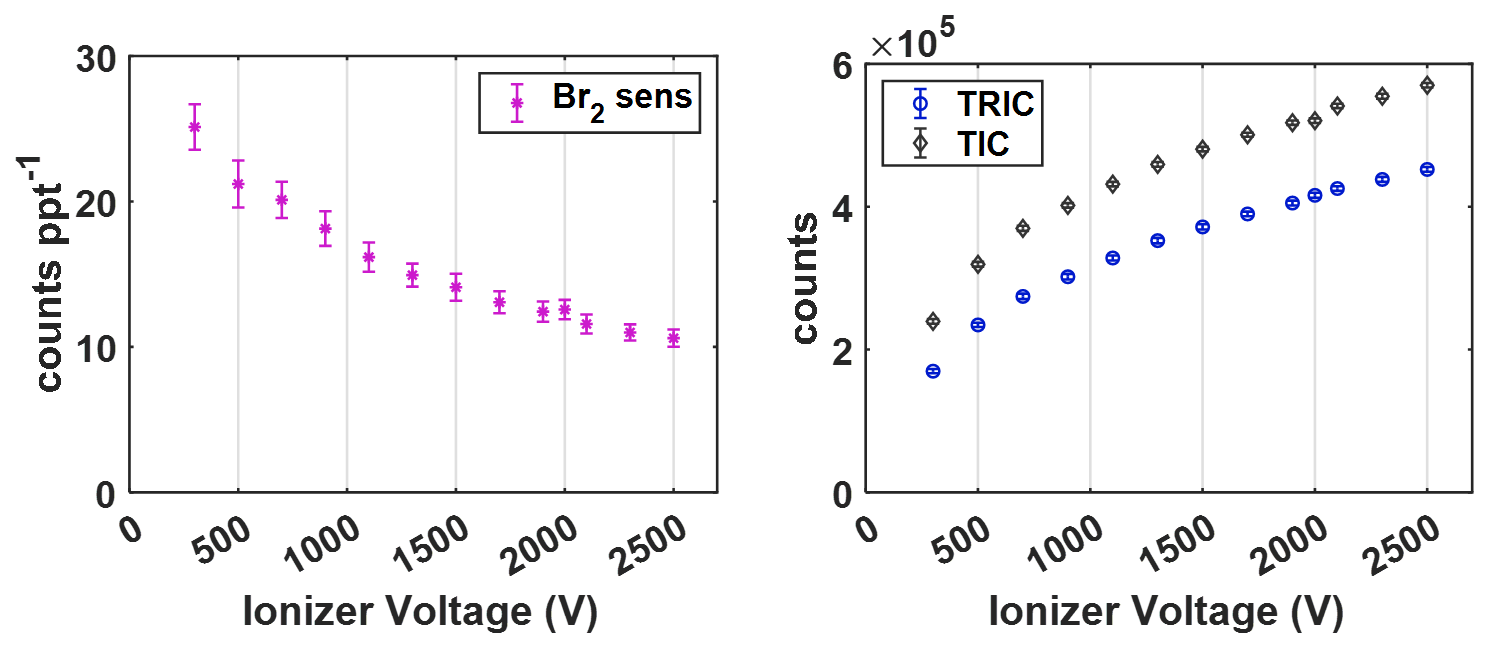
Figure 2 Br₂ average sensitivity (counts ppt⁻¹ per 10⁶ TRIC) vs. electric potential applied to VUV ionizer (left) and average TRIC and Total Ion Counts (TIC) vs. ionizer voltage (right).

4 Wall Effects

Another improvement with the transverse design of the t-IMR is the reduction of so-called wall effects. As mentioned in the introduction, wall or memory effects refer to compounds depositing onto IMR surfaces leading to both lower signals for species at the actual time of sampling as well as increased artificial signal later when molecules are liberated from surfaces and reintroduced in the sample flow. Reducing artificial signal is important for all CIMS applications, particularly for those wanting to measure low concentration species. Multiple laboratory studies have been conducted to quantify and reduce this unwanted effect across different IMRs and instrument techniques. Palm et al. (2019) showed that the fast zero technique in their new low pressure IMR significantly reduces memory effects quantified as the “instrument delay time”, which is defined as the time it takes for a specific compound's measured signal to return to 10 % of its value during a controlled addition to the IMR. In the same study, Palm et al. (2019) also provide a summary of how instrument delay time generally decreases with the calculated saturation vapor pressures and subsequent volatilities (or C^∗ values) of various compounds tested. In other words, less volatile species (lower C^∗) generally take longer to evaporate from IMR surfaces after deposition and will contribute to artificial signal for longer periods of time (longer instrument delay time). The lowest volatility species presented in this study had instrument delay times on the order of 10 min or longer. The goal for the t-IMR is to minimize this effect as much as possible by reducing molecule-surface interactions in the instrument.

To characterize our t-IMR in regard to wall effects, experiments were conducted to generate a suite of organic molecules covering a large range in volatility, via alpha pinene ozonolysis. The setup for this experiment is shown in Fig. A2. Ozone was generated by flowing approximately 4 L min⁻¹ of zero air from a Teledyne model 701 zero air generator through an enclosed cavity containing an ultraviolet lamp with output at 254 nm wavelength (Jelight #82-3309-9). Ozone concentrations registered between 900–1000 ppb in a glass flow tube where it was mixed with a 200 sccm flow of alpha pinene + UHP nitrogen gas. This resulted in a suite of organic products detected by the iodide CIMS, including various levels of oxygenated pinene products (i.e. C₁₀H₁₆O_x). The products were introduced to the t-IMR by manually moving a $\mathrm{1}/\mathrm{2}$ in. OD teflon tube outlet from the glass flow tube in front of either the t-IMR entrance or to exhaust. This output was moved in front of the t-IMR for 5, 10, and 30 s pulses repeatedly throughout the experiment to determine if sampling time influences instrument delay on these timescales.

Shown in Fig. 3 are the 1 Hz time series of thirty five alpha pinene ozonolysis products from this experiment during a representative 30 s pulse. Relative signals for each detected compound, normalized to their mean value during the 30 s pulse are shown colored by their oxygen-to-carbon atom ratios (O : C), indicating the least oxidized in green (O : C < 0.5) to most oxidized in purple (O : C > 1.5). Also plotted with red dashed lines is the value 0.1, representing the threshold corresponding to 10 % of the mean signal for each compound. The absolute signals measured corresponding to concentrations) for these products are consistent across the multiple additions and varied times, reaching the same level with each pulse. The signals drop to below their respective thresholds (red dashed line) on the order of 1–2 s after the products outflow tube was removed from the t-IMR, at 22:35:51 UTC (formatted as hh:mm:ss) as illustrated by the bottom plot of Fig. 3 showing a zoomed in view of the end of the 30 s pulse (highlighted in the grey dashed box for the top plot). Two representative organic molecular compositions are included in this plot: C₁₀H₁₆O₃, likely a collection of relatively high concentration semi-volatile products, and the much less volatile, more oxygenated products having a compoisition of C₁₀H₁₆O₈. These representative products of α-pinene ozonolysis span multiple orders of magnitude in volatility space. C^∗ values were calculated at temperatures of 298 K for these two compounds using their saturation vapor pressures as calculated and published by Hyttinen et al. (2022) using the SIMPOL methodology outlined by Pankow and Asher (2008). The C^∗ value determined for C₁₀H₁₆O₃ is 1.04×10³ µg m⁻³ and that of C₁₀H₁₆O₈ is 26 µg m⁻³ as an upper limit, and $\mathrm{1.7}\times {\mathrm{10}}^{-\mathrm{4}}$ µg m⁻³ as a lower limit. This experiment demonstrates that over a wide range of chemical volatility (and molar mass), instrument delay times remain between 1–2 s, consistent with inlet residence time. The instrument delay time is also demonstrated to be on the order of 1–2 s for an analogous experiment performed for nitric acid, HNO₃. The results of that experiment are shown in Fig. A3. Contextualizing these results with the summary of instrument delay time vs. saturation vapor pressure from Palm et al, the atmospheric pressure t-IMR demonstrates significant improvement in reduction of wall memory effects for lower volatility organic compounds, with instrument delay time on the order of 1 s, much less than the ∼10-minutes reported for low pressure designs. This result is also comparable if not an improvement to the e-folding time (time for signal to drop to 36 % signal) of 1s calculated for the crossflow design presented by Zhao et al. (2017) for nitric acid.

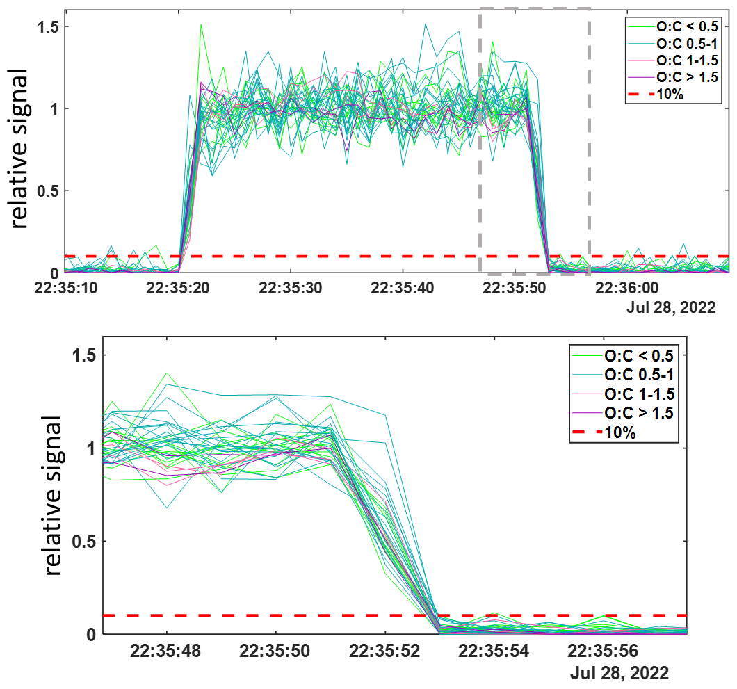
Figure 3 1 Hz time series of 35 α-pinene ozonolysis products generated in a laboratory study and detected in the t-IMR. Compounds shown colored by O : C ratio and reported in normalized signals relative to the averaged detected during addition. Relative 10 % signal lines shown in red. Bottom plot shows zoomed in view of time series as shown in grey box of top plot.

5 In-Situ Observations

The t-IMR was deployed to the field as part of the Bermuda boundary Layer Experiment on the Atmospheric Chemistry of Halogens (BLEACH). The BLEACH campaign took place over two six-week periods from May–June 2022 and January–February 2023. The results presented here will focus on the latter winter leg of the measurements. The t-IMR CIMS was stationed at the Tudor Hill Marine Atmospheric Observatory (THMAO) located on the southwestern shores of Bermuda and operated by the Bermuda Institute of Ocean Sciences (BIOS). The CIMS sampled from atop a 10 m tower on the shore and was contained in weatherproof housing with an attached air conditioner to assist in stabilizing instrument temperatures. To both accelerate ambient air to the IMR chamber as well as shield the inlet from precipitation and high winds, a 3 in. diameter secondary inlet was sealed around the 1 in. t-IMR chamber and was pumped at 110 L min⁻¹, of which 10 L min⁻¹ was sub-sampled by the t-IMR with the same setup of 1.5 kV applied electric potential and iodide ionization scheme described in the previous sections. The additional residence time from this 3 in. secondary inlet at such a pumping speed is calculated to be 0.76 s. which brings the total residence time for ambient molecules to 1.5 s from entering the outer inlet to the pinhole CIMS entrance. Background signals for a given compound were determined by taking the average signal for that compound during a “zero period” where a flow of 14 L min⁻¹ of the UHP N₂ gas overflowed the t-IMR by way of a mass flow controller output manually placed in front of the 1 in. inlet (within the larger 3 in. sheath inlet). These signals are characterized by a local minimum in the H₂OI⁻ signal, as the ionization region is being overflowed with virtually completely dry nitrogen gas as opposed to the more humid ambient conditions. This “zero” signal is then averaged between multiple overflow periods throughout the campaign and subtracted from the corresponding ambient counts for that detected species. LOD is also calculated using signals recorded during zero periods according to the equation from Bertram et al, giving detection limits on the order of tens of ppq for certain low concentration halogenated species on a 1 min integration timescale, including HOBr. These values are presented in Table A1. In calculating LOD, we use background signals and sensitivity values that are not normalized to Total Reagent Ion Counts (TRIC = I⁻ + IH₂O⁻ signals). In the case of Br₂ these parameters are, respectively, 0.48 counts and 8.1 counts ppt⁻¹, which along with the 60 s integration time and a set signal-to-noise ratio of 3, gives the reported LOD of 0.06 ppt. The t-IMR CIMS in iodide mode is capable of measuring multiple reactive halogen species as well as a suite of organic molecules in the ambient conditions at the site. Shown in Fig. A5 is the 1 min time series of I⁻ and IH₂O⁻ signals to demonstrate the dynamic humidity conditions in the t-IMR during the deployment.

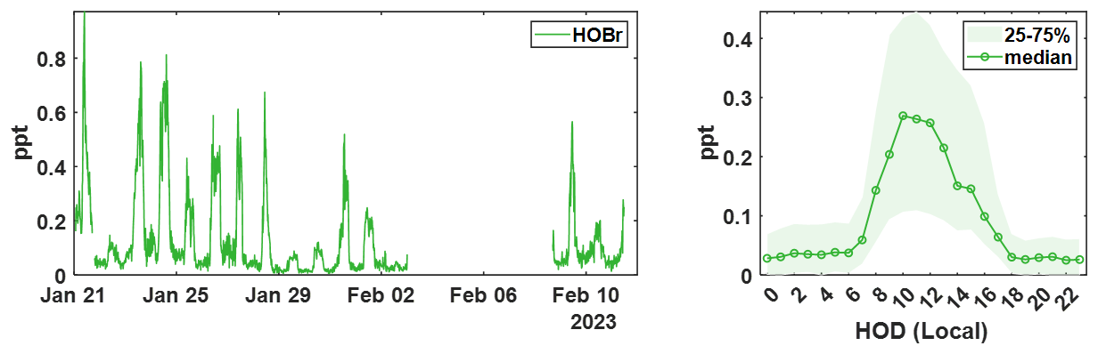
Figure 4 15 min averaged time series of ambient (water-vapor-corrected) HOBr concentrations measured during the winter BLEACH campaign (left) and the diurnal profile showing median signal at each hour of day (HOD) in local time (right). Shading indicates the bounds of the 25th and 75th quartiles for the measured concentrations in each hourly bin.

Shown in Fig. 4 is the time series as well as the diurnal profile for ambient HOBr measured during the winter BLEACH campaign. Median concentrations are shown in the open circle trace for the diel cycle, with shading representing the 25th and 75th percentiles for the entire sampling period. This data is the result of peak-fitting and integrating 1 min pre-averaged spectra from the t-IMR CIMS, after which further binning is performed to give a 15 min data frequency. The time series is quality controlled to exclude any calibrations, zeros, or instrument maintenance. Quantum model simulations to calculate the binding enthalpies (BE) to the reagent I⁻ for each of these molecules were performed, as these values correlate with and therefore may be used as a proxy for the relative sensitivities between these species (Iyer et al., 2016). Geometries of the free molecules and the molecular clusters are optimized at the PBEPBE/aug-cc-pVTZ-PP level of theory using the Gaussian 16 program (Perdew et al., 1996; Kendall et al., 1992; Frisch et al., 2016). Iodine and bromine pseudopotential definitions are taken from the Environmental Molecular Sciences Laboratory (EMSL) basis set library. The final energies are refined at the DLPNO-CCSD(T)/def2-QZVPP level of theory using the ORCA program version 4.2.1 (Feller, 1996; Peterson et al., 2003; Riplinger et al., 2013; Riplinger and Neese, 2013; Weigend and Ahlrichs, 2005; Neese, 2012). The calculated BEs are 24.3 and 15.1 kcal mol⁻¹, respectively for Br₂ and HOBr. Regular calibrations for Br₂ performed throughout the campaign using the same permeation device described in Sect. 3 are used to produce a general sensitivity value for the t-IMR CIMS, which is used for the conversion of instrument signal counts to atmospheric concentration (ppt). In the study by Iyer et al. (2016), a linear correlation is found between the logarithm of iodide-reagent CIMS sensitivity and calculated binding enthalpy for a given compound, $\log C_{f,X}\propto \mathrm{\Delta }{H}_X$ (where C_f,X is the instrument sensitivity and ΔH_X is the binding enthalpy for measured compound X). Using the binding enthalpies and the measured Br₂ sensitivity during calibration, we calculate HOBr sensitivity:

$$\begin{array}{}\text{(2)}& {\displaystyle \frac{\log C_{f,\mathrm{HOBr}}}{\log C_{f,{\mathrm{Br}}_{\mathrm{2}}}}}={\displaystyle \frac{\mathrm{\Delta }{H}_{\mathrm{HOBr}}}{\mathrm{\Delta }{H}_{{\mathrm{Br}}_{\mathrm{2}}}}}\Rightarrow C_{f,\mathrm{HOBr}}=C_{f,{\mathrm{Br}}_{\mathrm{2}}}^{\left(\frac{\mathrm{\Delta }{H}_{\mathrm{HOBr}}}{\mathrm{\Delta }{H}_{{\mathrm{Br}}_{\mathrm{2}}}}\right)}\end{array}$$

Sensitivity values calculated using this method for halogenated species detected during BLEACH23 are presented in Table A1, along with the directly measured Br₂ and HNO₃ sensitivities.

It has been reported in multiple studies that CIMS sensitivity to several classes of compounds is dependent on the humidity, or more specifically, the partial pressure of water vapor ($P_{{\mathrm{H}}_{\mathrm{2}}\mathrm{O}}$) present in the IMR during sampling, which is also related to temperature and pressure (Krechmer et al., 2018; Kercher et al., 2009; Dörich et al., 2021; Zaytsev et al., 2019). We developed a dynamic $P_{{\mathrm{H}}_{\mathrm{2}}\mathrm{O}}$-based sensitivity correction for Br₂ and HNO₃ using laboratory experiments, which is used in conjunction with the direct in-field Br₂ calibrations to generate dynamic sensitivity values for halogen-containing species detected during BLEACH23 (see Appendix B). Integrated signal counts for these compounds (clustered to the iodide reagent) are normalized to TRIC and subsequently divided by the corresponding sensitivity time series, point-by-point, to produce concentration values reported in parts per trillion (ppt) by volume at each 1 min time step. The daily maximum levels of HOBr vary throughout the campaign, but concentrations reliably increase during daylight hours roughly between 07:00 and 17:00 UTC during the winter in Bermuda, corresponding to within the hours of sunrise and sunset for THMAO in Jan-Feb. This aligns with the current understanding of the bromine chemical mechanism in that most gas-phase production of HOBr in the atmosphere requires photochemical reactions (Zhang et al., 2023; Swanson et al., 2022).

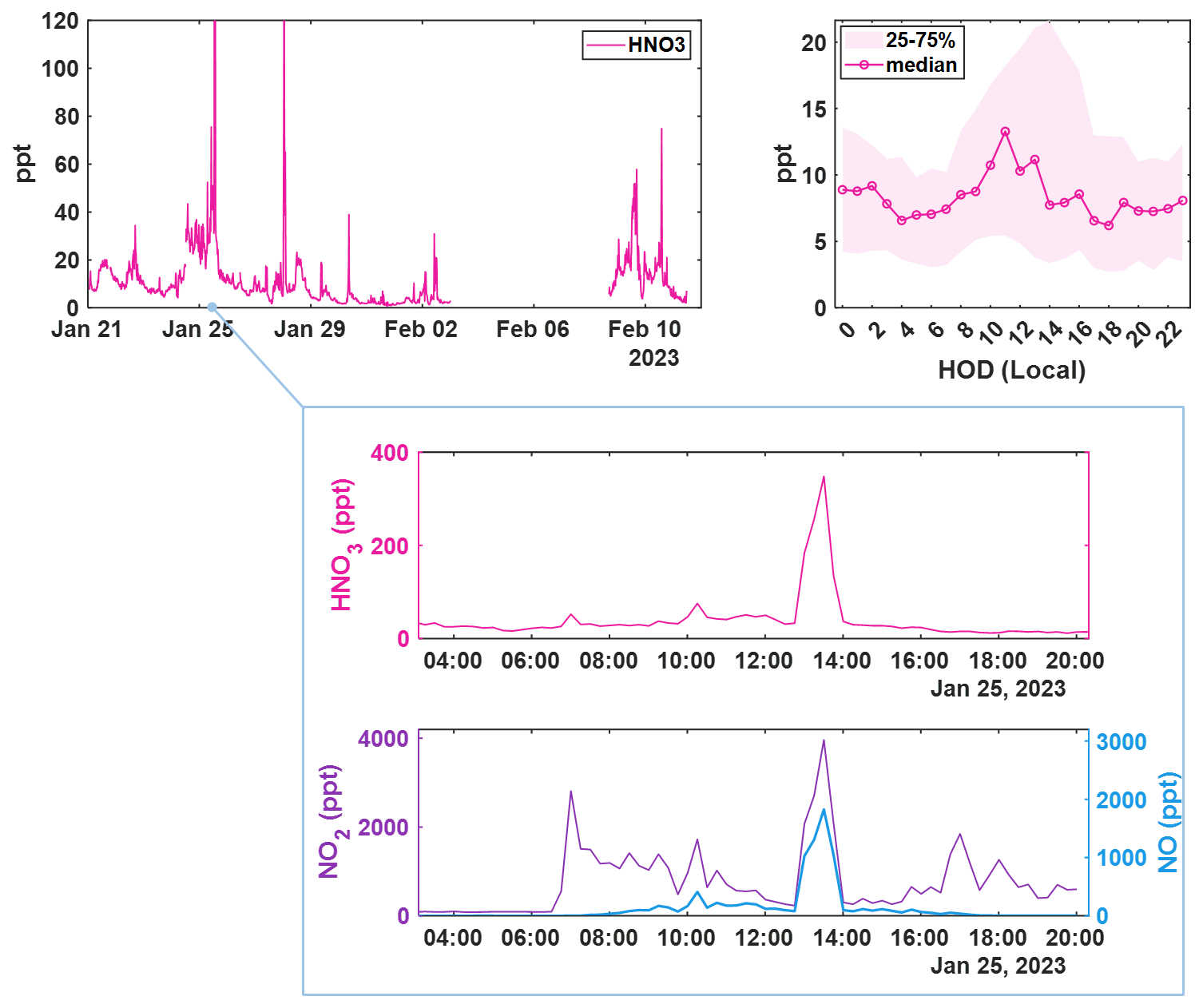
Figure 5 15 min averaged time series of ambient HNO₃ concentrations measured during the winter BLEACH campaign (top left), corrected for IMR water vapor concentrations and the diurnal profile showing mean signal at each hour of day (HOD) in local time (top right). Shading indicates the bounds of the 25th and 75th quartiles for the measured concentrations in each hourly bin. A zoomed in view of a spike (middle) in HNO₃ concentration as measured by CIMS coinciding with (bottom) measurements of NO (blue, right axis) and NO₂ (purple, left axis) as detected by a Laser-Induced Fluorescence (LIF) instrument.

Shown in Fig. 5 is the time series and diel cycle for measured nitric acid concentrations (HNO₃), corrected for humidity changes in the t-IMR. Similarly to those of the HOBr data, 1 min averaged spectra were integrated to produce signal counts, and a sensitivity at the time of in-field Br₂ calibration is determined via binding enthalpies. The BE for HNO₃ is published as 21.52 kcal mol⁻¹ (Iyer et al., 2016). The HNO₃ sensitivity using the BE method is calculated to be 1.4 counts ppt⁻¹. Details about the water vapor correction of HNO₃ can be found in Sect. B. What was determined to be a small contamination of nitric acid on tubing connections involved during zero periods in the BLEACH campaign made it such that the HNO₃ time series could not be background subtracted, though all other quality controls used in the HOBr data are applied here. The diurnal cycle shows median concentrations increasing during daytime hours evident in the shading of the 75th percentile measurements, with a particular period of higher median values in the morning. The relatively elevated concentrations during the day are consistent with the main gas phase production of HNO₃ coming from reaction of NO₂ with OH, requiring photochemistry. This is evidenced by the bottom two plots shown in Fig. 5 which show a zoomed in view of a peak in HNO₃ (cutoff by axis limits in the complete time series for clarity) accompanied by NO and NO₂ concentrations on the bottom plot as measured by a Laser-Induced Fluorescence (LIF) instrument (Rollins et al., 2020). The largest spike in HNO₃ coincides with similar very large spikes in both NO and NO₂, indicative of both high total NO_x and active photolysis. However, there are periods during the night in which HNO₃ is generally elevated and also episodically peaks in concentration. This is likely indicative of nighttime production pathways, presumably hydrolysis of N₂O₅ with H₂O on aerosol surfaces and/or NO3 reactions with dimethyl-sulfide (DMS) or volatile organic compounds (VOCs) (Brown et al., 2004; Reed et al., 2017). Shown in Fig. A6 is a representative overnight time series of HNO₃, NO_x, and ClNO₂ concentrations as well as N₂O₅ signal counts to illustrate this point. Representative mass spectra showing peak fits for both HOBr and HNO₃ as measured with the iodide CIMS are shown in Fig. A4. These in-situ observations demonstrate the capability of the t-IMR to not only be deployed to the field, but also to measure a diverse suite of compounds down to sub-ppt concentrations while minimizing wall effects and instrument residence time.

6 Conclusions

In this work we have characterized a novel atmospheric-pressure IMR inlet (t-IMR) for use with CIMS applications. The crossflow t-IMR is shown to operate under laminar flow conditions with an electric field used to accelerate reagent ions and subsequent ion-ambient molecule clusters across the relatively high-pressure, high flow space to be sampled by the CIMS, resulting in much higher observed ion signals compared to measurements with no applied field, typically by two orders of magnitude. The standard operating electric potential is optimized to retain high total ion signal while also maximizing measured sensitivity. The t-IMR design is also shown to reduce wall memory effects compared to previously studied low-pressure designs, decreasing instrument delay times from the order of minutes to the order of 1 s for a representative suite of varied volatility organic gases. This increases the measurement reliability of ambient gases even at relatively lower volatilities, particularly improving detection of low concentration species. Results from the first field deployment of the t-IMR demonstrate the capability of the design to sample ambient trace gases continuously, down to sub-ppt concentrations in the case of HOBr.

Operating with the atmospheric pressure t-IMR shows several clear advantages, but also introduces some limitations, including less control over ambient pressure and humidity changes. While the high flow through the IMR chamber reduces wall interactions and residence time, this does present potential difficulty in background determinations as overflowing with 10 or more L min⁻¹ of UHP nitrogen gas can be difficult in certain settings where specialty gas quantities are limited. The relatively high sample flow rate also makes it difficult to humidify such a “zero” in applications where a non-dry zero is desired, i.e. with a water bubbler. Since CIMS sensitivity to many compounds has been shown to be somewhat dependent on the amount of water vapor present in the IMR, it is important to quantify the humidity-dependence of sensitivities measured with the t-IMR design. It would also be useful in the future to conduct a sensitivity study for the multitude of organic species that have been measured by iodide reagent chemistry with other IMR designs and conditions for inter-comparison purposes.

Appendix A

Table A1 Limits of detection for halogenated species detected during BLEACH (calculated for 1 min integration time) and corresponding average sensitivity values (C_f,X) based on direct in-field Br₂ calibration and Eq. (2).

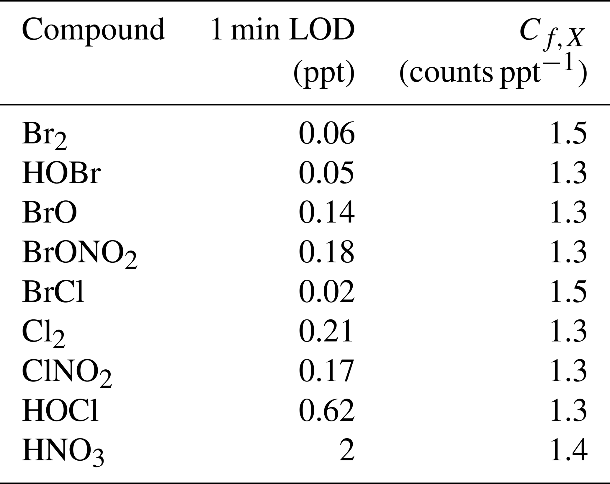
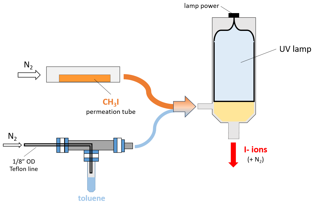
Figure A1 A diagram showing the VUV setup for I⁻ ion production. UHP N₂ is flown over both a CH₃I permeation tube at 1.5 L min⁻¹ (orange) and the headspace of a liquid toluene vial at 2 sccm (0.002 L min⁻¹, light blue), which combine and enter the VUV cavity illuminated by the UV lamp represented with yellow shading. Resulting I⁻ ions exit the VUV housing at a stainless $\mathrm{1}/\mathrm{4}$ in. OD port where an electric potential is applied.

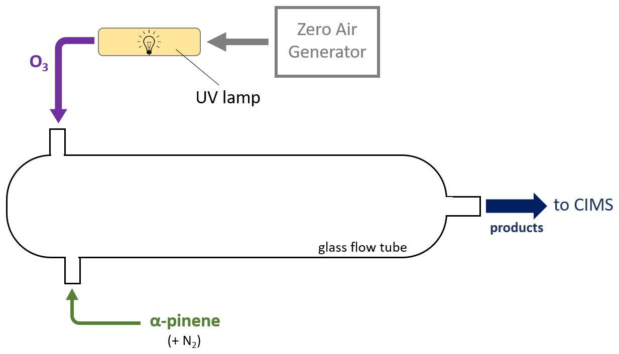
Figure A2 Setup schematic for the alpha-pinene ozonolysis wall effects experiment. A 4 L min⁻¹ flow from the zero air generator is passed through a chamber illuminated by UV light to produce O₃ which is input into a glass flow tube (purple) along with a 200 sccm (0.200 L min⁻¹) flow of gaseous alpha pinene + UHP N₂ (green). Gases mix to form products (dark blue) which are output into the transverse IMR-equipped CIMS.

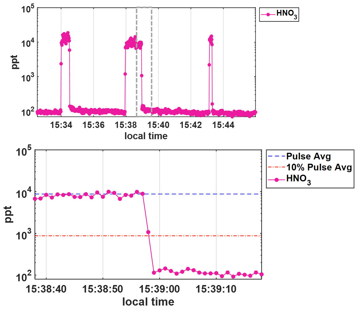
Figure A3 1 Hz HNO₃ concentrations in ppt shown on a log scale during wall effects experiment where (top) HNO₃ is added to the t-IMR in pulses of 20, 60, and 10 s, respectively. The bottom panel shows a zoomed in view (gray dashed box in the top plot) of the 60 s pulse, showing that concentrations return to below 10 % (orange dash line) of the average concentration during addition (blue dash line) on the order of 1–2 s.

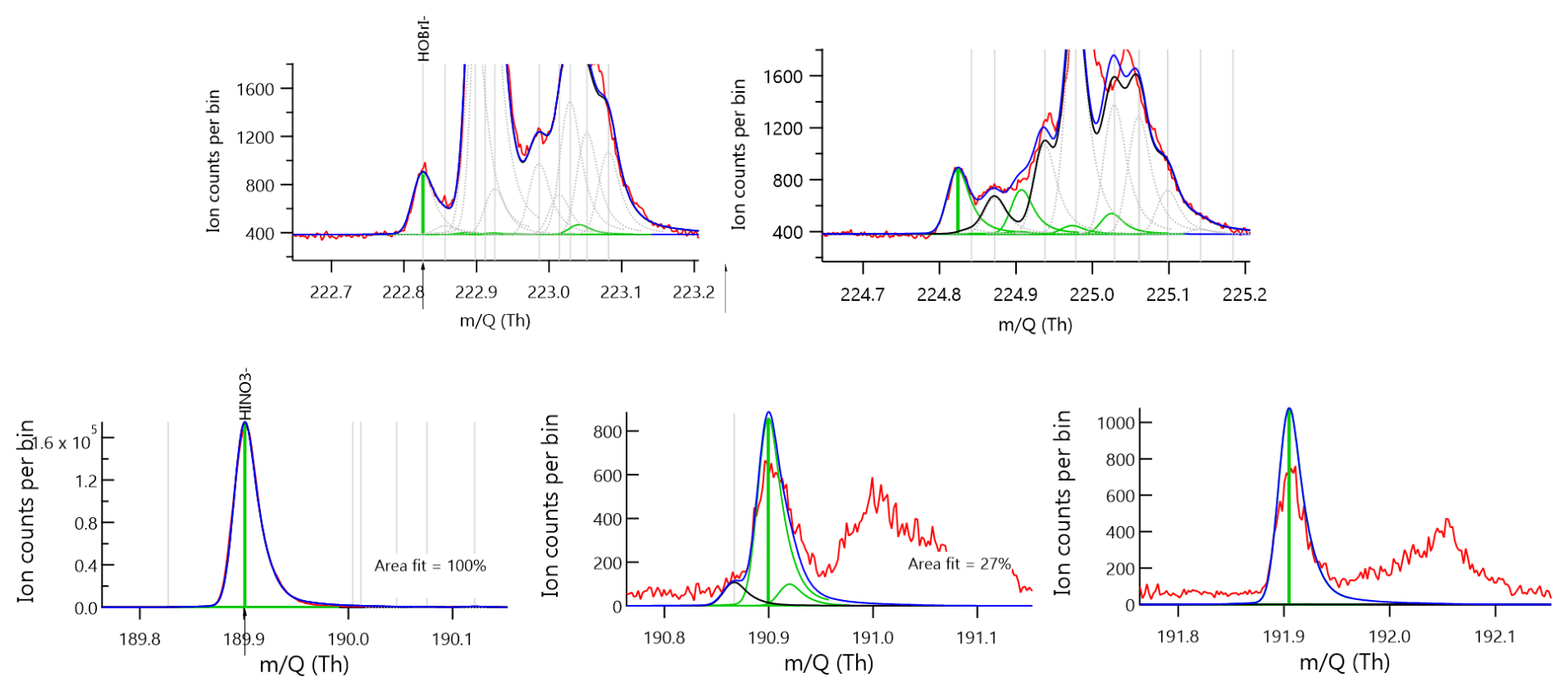
Figure A4 Approximately 15 min integrated mass spectra showing signal in ion counts vs. mass to charge ratio ($m/Q$). Red traces indicate raw data while the dark blue show fitted and assigned peaks using an adjusted Gaussian model. Green bars indicate the mass-to-charge positions and fitted intensities for chemical compositions (top) HOBr and (bottom) HNO₃ when clustered to I⁻. The additional plots to the right show fits for the respective isotopes, m+2 for HOBr and both m+1 and m+2 for HNO₃.

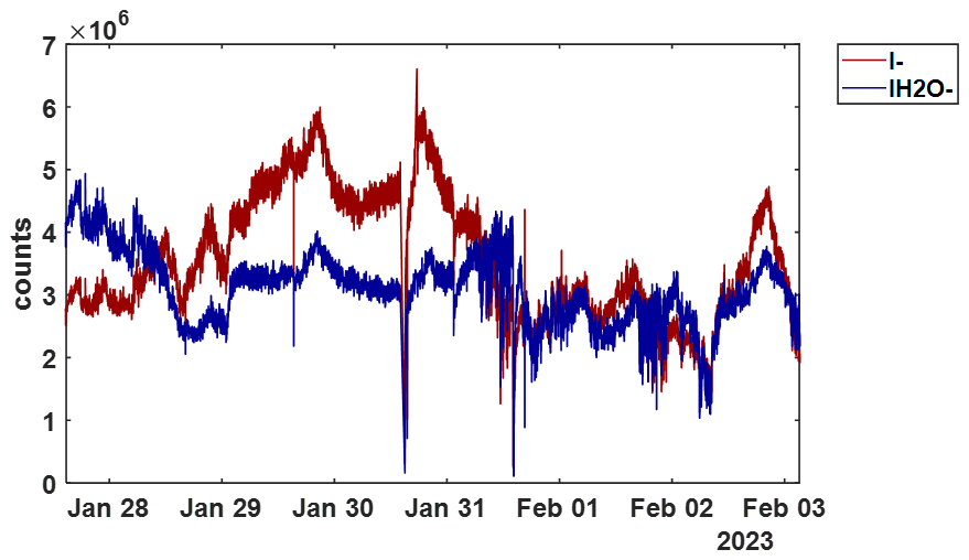
Figure A5 1 min resolved time series of I⁻ (red) and IH₂O⁻ (blue) signals during the BLEACH23 campaign to demonstrate dynamic conditions with the t-IMR equipped CIMS.

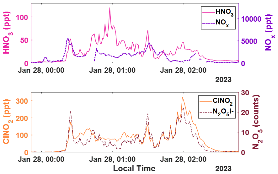
Figure A6 Representative 1 min time series of (top) HNO₃ and NO_x concentrations in magenta and purple dashes, respectively; as well as (bottom) ClNO₂ concentrations and signal counts of N₂O₅, respectively in orange and dark red dashes. The concentrations and signals of all but HNO₃ are background subtracted.

Appendix B: Humidity-based sensitivity Correction

During the wintertime BLEACH campaign, temperatures ranged from a minimum of 16 °C to a maximum of 23 °C and humidity from 51 %–98 %, which combine to give the $P_{{\mathrm{H}}_{\mathrm{2}}\mathrm{O}}$ range of 10 to 25 mbar at ambient pressures on the order of 1 atm (1013.25 mbar). As previously mentioned, the ambient humidity is assumed to equivalent to that inside the IMR throughout ambient sampling, which includes periods of direct Br₂ calibration where RH ranged between 68 %–77 %, which translates along with temperature to $P_{{\mathrm{H}}_{\mathrm{2}}\mathrm{O}}$ values spanning 16.9–17.5 mbar. This is a relatively small window of water vapor pressures during calibration, thus it is important to quantitatively determine the $P_{{\mathrm{H}}_{\mathrm{2}}\mathrm{O}}$ dependence of bromine sensitivity.

This extrapolation is accomplished using a post-campaign laboratory experiment during which Br₂ is delivered to the IMR at a constant rate from the same permeation device deployed during BLEACH. Upstream of the bromine gas output, the humidity (and thus water vapor pressure) in the IMR is modulated via the addition of UHP N₂ that is both unaltered (dry) and passed through a room temperature bubbler where water is held in an air-tight flask with two ports for N₂ input (below water level) and humidified output. The dry and humidified N₂ gas are carried into t-IMR at varying relative flow rate fractions, with the sum of both remaining constant at 7 L min⁻¹. Several minutes are elapsed after step changes in the dry and humidified flows, to allow sufficient time for humidity and Br₂ ion signals to stabilize. Only data during these equilibrated periods (i.e. the final 1–2 min) are used for sensitivity analysis. Humidity in the t-IMR during laboratory experiments is measured downstream of the ion flow/MS sampling port in the exhaust line using the probe of an Elitech model GSP-6 temperature and humidity logger, positioned upstream of the IMR pump.

Shown in Fig. B1 is the resulting Br₂ sensitivity in counts ppt⁻¹ (per 10⁶ TRIC) scattered against partial water vapor pressure (in mbar), as calculated using measured humidity, temperature, and a constant pressure of 1 atm. Both horizontal and vertical error bars represent one standard deviation in observed $P_{{\mathrm{H}}_{\mathrm{2}}\mathrm{O}}$ and sensitivity, respectively. Data from the experimental setup described above are shown with blue markers and labeled as “Lab”. Data from direct calibration during the winter 2023 and summer 2022 BLEACH campaigns are shown in black and red, respectively, with $P_{{\mathrm{H}}_{\mathrm{2}}\mathrm{O}}$ in these cases calculated using the humidity, temperature, and pressure measurements at THMAO. A modified gaussian fit is applied to all data from the laboratory and BLEACH campaigns, shown in purple. The equation for this modified gaussian fit extrapolates from previous work from Lee et al. (2014), which determined bromine sensitivity for a low pressure IMR ($P_{{\mathrm{H}}_{\mathrm{2}}\mathrm{O}}<\mathrm{1}$) and another study from Zhao et al. (2017), reporting that sensitivities for multiple compounds decay at a decreasing rate above a water vapor pressure threshold on the order of 10 mbar. The resulting fit equation has the format:

$$\begin{array}{}\text{(B1)}& \begin{array}{rl}y=& k_{\mathrm{1}}+k_{\mathrm{2}}\log \left({\displaystyle \frac{x}{k_{\mathrm{3}}}}\right)+k_{\mathrm{4}}\exp \left(-(k_{\mathrm{5}}\cdot x+k_{\mathrm{6}})\right)\\ & \cdot \exp \left({\left({\displaystyle \frac{-(x-k_{\mathrm{7}})}{k_{\mathrm{8}}}}\right)}^{\mathrm{2}}\right)+k_{\mathrm{9}}\exp (-k_{\mathrm{10}}\cdot x)\end{array}\end{array}$$

where y corresponds to Br₂ sensitivity, x to $P_{{\mathrm{H}}_{\mathrm{2}}\mathrm{O}}$, and k_1–10 representing constant fit parameters.

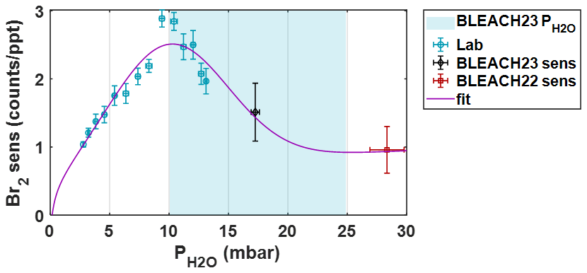
Figure B1 Bromine sensitivity vs. partial pressure of water vapor ($P_{{\mathrm{H}}_{\mathrm{2}}\mathrm{O}}$) with data determined from the post-campaign laboratory experiment (blue), and direct calibrations from the winter BLEACH23 (black) and summer BLEACH22 (red) campaigns. A custom modified-Gaussian fit using all data points is shown in purple. Blue shading indicates the range of $P_{{\mathrm{H}}_{\mathrm{2}}\mathrm{O}}$ calculated from measured temperature and humidity during BLEACH23 (10–24 mbar).

The fit shows an initial increase in sensitivity with increasing $P_{{\mathrm{H}}_{\mathrm{2}}\mathrm{O}}$, plateauing and reaching a maximum at approximately 10.3 mbar, followed by a slower decline to a slightly positively sloped asymptote with a value around 0.9–1 counts ppt⁻¹ at higher humidities/vapor pressures. There is also a decline in sensitivity to 0 at a partial water vapor pressure of 0.1 mbar, which would give (non-real) negative sensitivity values for a completely dry sample. Though during ambient sampling in the t-IMR operating at atmospheric pressure, $P_{{\mathrm{H}}_{\mathrm{2}}\mathrm{O}}$ values are not expected to register near this range. This is especially apparent during the BLEACH23 campaign, where the water vapor pressure values never fall below 10 mbar, as mentioned previously. Therefore, this potentially problematic lower boundary does not affect the humidity-dependent sensitivity correction for the BLEACH campaign measurements or those carried out in the laboratory.

The modified gaussian fit is used to generate a dynamic sensitivity value for Br₂. We apply this water vapor dependence to other halogen-containing species (i.e. HOBr, for which we assume a similar relationship to $P_{{\mathrm{H}}_{\mathrm{2}}\mathrm{O}}$) by using the directly measured Br₂ sensitivity value and Eq. (2). The fit equation for Br₂ is normalized to a value of 1 at the point of average $P_{{\mathrm{H}}_{\mathrm{2}}\mathrm{O}}$ for in-field calibrations, and then multiplied by the sensitivities of the other compounds calculated using their respective binding enthalpy ratios. Scaling sensitivity to other compounds at the point of Br₂ calibration periods before applying the $P_{{\mathrm{H}}_{\mathrm{2}}\mathrm{O}}$ correction ensures that the conversion for all (halogenated) compound signals to concentration from ion signal is based on a direct, in-situ sensitivity measurement under identical conditions. Humidity and temperature measurements at THMAO have the same 1 min resolution as the pre-averaged CIMS data, resulting in a 1-to-1 time series match of $P_{{\mathrm{H}}_{\mathrm{2}}\mathrm{O}}$ and thus 1 min resolved humidity-corrected sensitivity values.

A similar experiment is performed while delivering HNO₃ to the t-IMR, again while modulating humidity with a combined dry and bubbler flow. The experiment utilizes a custom made permeation device where concentrated nitric acid fills a permeable PTFE tube sealed at each end with solid PTFE caps. In this case, there are no in-field calibrations to extend available data to higher $P_{{\mathrm{H}}_{\mathrm{2}}\mathrm{O}}$ values. The results are shown in Fig. B2 with experimental data shown in blue. An exponential fit is applied (shown in purple in the figure), with an R² value of 0.98 and equation formatted as $y=a{e}^{-bx}$, where y corresponds to HNO₃ sensitivity, x to $P_{{\mathrm{H}}_{\mathrm{2}}\mathrm{O}}$, with a and b as constants. This fit (and the experimental data shown) are normalized such that the sensitivity is equal to 1 for the average $P_{{\mathrm{H}}_{\mathrm{2}}\mathrm{O}}$ during calibrations (= 17.3 mbar). As with HOBr, the sensitivity is calculated at each time step using $P_{{\mathrm{H}}_{\mathrm{2}}\mathrm{O}}$ measurements, this normalized fit, and the HNO₃ sensitivity based on in-field Br₂ calibrations and BEs. This time series of sensitivity is then used to convert signals to concentration.

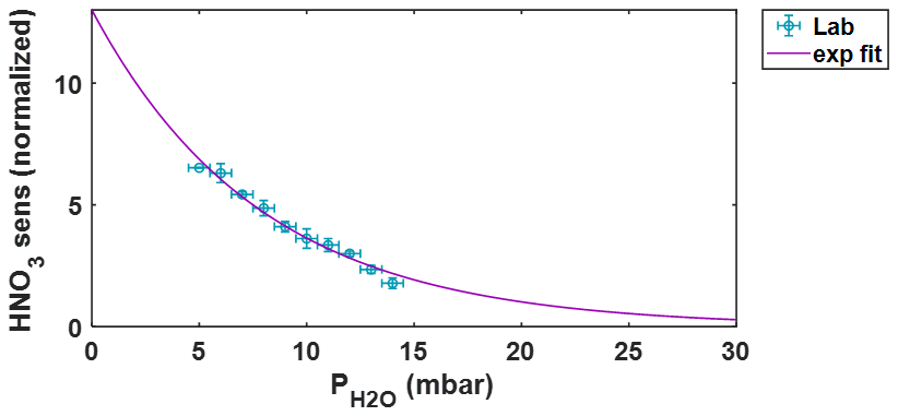
Figure B2 HNO₃ sensitivity vs. partial pressure of water vapor ($P_{{\mathrm{H}}_{\mathrm{2}}\mathrm{O}}$) from a laboratory experiment (blue). An exponential fit using all data points is shown in purple. Data are normalized so that the sensitivity is equal to 1 at $P_{{\mathrm{H}}_{\mathrm{2}}\mathrm{O}}$ = 17.3 mbar, the average during in-field calibration.