The ASK-16 motorized glider: an airborne eddy covariance platform to measure turbulence, energy, and matter fluxes

Airborne eddy covariance measurements can bridge the gap between local (tower-based) and regional (satellite/inversion-derived) flux data, as they provide information about the spatial distribution of turbulent fluxes for larger regions. Here, we introduce an airborne eddy covariance measurement platform based on an ASK-16 touring motor glider (TMG; also referred to as a power glider, hereafter referred to as motorized glider), which is equipped to measure the three-dimensional (3D) wind vector, and atmospheric conditions, and we derive airborne turbulent fluxes for the use of measurement campaigns over European landscapes. This study describes the measurement setup of the platform and explains the workflows that were used to calculate and calibrate the 3D wind vector, turbulent fluxes, and their associated source areas. The glider is equipped with an 858 AJ Rosemount five-hole probe, a Picarro G2311-f gas analyzer, a Novatel FlexPak G2-V2 GNSS–INS system, Vaisala temperature and humidity sensors (HMT311), and an OMEGA CHAL-003 thermocouple temperature sensor. Measurement data are processed with PyWingpod (Python) and eddy4R (R) software packages to calculate wind vectors and turbulent fluxes and assign footprints to the calculated fluxes. To evaluate the quality of the obtained fluxes, different quality assessments have been performed, including the determination of detection limits, spectral analysis, stationarity tests, the analysis of integral turbulence characteristics, and measurement noise and error evaluation. The uncertainty of w is between 0.15 and 0.27 m s⁻¹ (median = 0.23 m s⁻¹), and the uncertainty of u and v ranges between 0.16 and 0.55 m s⁻¹ (median = 0.25 m s⁻¹). Analysis of exemplary flux data from flight transects indicates that the platform is capable of producing spatially highly resolved turbulent fluxes over heterogeneous landscapes. Overall, results from our analysis suggest that the ASK-16 airborne platform can measure turbulent fluxes with a similar quality to earlier established high-quality platforms.

1 Introduction

Eddy covariance is the standard method to quantify the exchange of energy and matter fluxes in the atmospheric boundary layer (Baldocchi, 2003; Rebmann et al., 2018) and to understand their environmental drivers (e.g., Jung et al., 2020; Xu et al., 2017). Deployed from flux towers, eddy covariance provides observations with a high temporal resolution, but the spatial coverage of these observations is limited (Kaharabata et al., 1997). Airborne eddy covariance measurements, on the other hand, can quantify fluxes from local to regional scale (e.g., Hannun et al., 2020; Metzger et al., 2013; Serafimovich et al., 2018; Zulueta et al., 2011) and can additionally capture dispersive fluxes (Metzger et al., 2021; Wolfe et al., 2018). Therefore, airborne eddy covariance measurements provide a perfect base to complement tower measurements and can be combined with tower data to gain information content (Metzger et al., 2021; Zulueta et al., 2011). In addition, airborne measurement systems provide high spatial flexibility and provide the opportunity to measure turbulent fluxes in landscapes that are normally difficult to access (e.g., Tetzlaff et al., 2015).

To date, a large variety of airborne eddy covariance platforms have been developed. The first platforms already measured turbulent fluxes more than 40 years ago (Desjardins et al., 1982; Lenschow et al., 1980). Over time, airborne flux measurement systems have evolved with the development of (1) modern measurement equipment (e.g., O'Shea et al., 2013a; Wolfe et al., 2018), (2) flux quality assessment methods (Vellinga et al., 2013; Vickers and Mahrt, 1997; Mann and Lenschow, 1994), and (3) flight pattern optimization (Metzger et al., 2021; Vihma and Kottmeier, 2000), as well as (4) the inclusion of wavelets in the flux calculation to obtain spatially highly resolved fluxes (Mauder et al., 2007; Metzger et al., 2017). Nowadays, modern airborne flux platforms can provide eddy covariance fluxes that are similar to high-quality data from flux towers (e.g., Gioli et al., 2004). Operating platforms for airborne eddy covariance measurements include helicopter-borne turbulence probes (Helipod; Bange et al., 2006), weight-shift microlight aircraft (Metzger et al., 2012; Metzger, 2013), drones (Sun et al., 2021), and different research aircraft (e.g., the NRC Twin Otter – Desjardins et al., 2016; Sky Arrow ERA – Gioli et al., 2006; Polar 5 – Hartmann et al., 2018; FAAM BAe-146 – O'Shea et al., 2013b; NASA C-23 Sherpa – Wolfe et al., 2018; MetAir Diamond – Neininger et al. 2001)

Commonly, airborne eddy covariance campaigns focus on measuring sensible heat fluxes, latent heat fluxes, and carbon fluxes in landscapes ranging from being relatively homogeneous to highly complex (e.g., Bange et al., 2006; Kirby et al., 2008; Metzger et al., 2013; Wolfe et al., 2018; Zulueta et al., 2013; Kohnert et al., 2017). A few airborne platforms have additionally been equipped with methane gas analyzers to obtain methane fluxes for various landscapes, including agricultural fields in Switzerland (Hiller et al., 2014), arctic permafrost regions in Canada (Mackenzie Delta; Kohnert et al., 2017, 2018) and Alaska (Serafimovich et al., 2018; Zona et al., 2016; Sayres et al., 2017; Chang et al., 2014), wetlands (O'Shea et al., 2013b; Hannun et al., 2020), gas extraction sites (Yuan et al., 2015), and agricultural landscapes (Desjardins et al., 2018; Hannun et al., 2020; Wolfe et al., 2018). Additional airborne eddy covariance campaigns have been performed to determine the regional fluxes of nitrogen oxides (NO_x) in London (Vaughan et al., 2016, 2021), regional fluxes of volatile organic compounds (VOCs) in Mexico City (Karl et al., 2009) and London (Vaughan et al., 2017), and regional ozone fluxes near Boulder (Lenschow et al., 1980). Overall, these examples show that airborne eddy covariance platforms are successful at providing regional turbulent fluxes of various compounds in a large variety of landscapes.

In this study, we equipped a Schleicher ASK-16 touring motor glider (operated by the Freie Universität Berlin, Germany) with sensors to measure turbulent fluxes of carbon, methane, and energy at the regional scale. This new measurement platform enables a variety of research opportunities, including

• 1.

  studying the comparability of tower fluxes and airborne fluxes and the spatial representativeness of eddy covariance towers,

• 2.

  studying the regional spatial distributions of energy and matter fluxes and their dominating (spatial) drivers, and

• 3.

  applying and developing upscaling approaches to create regional-scale surface flux maps.

Additionally, several location-specific measurement flights were recorded between 2017 and 2022 to (1) study carbon and methane fluxes over differently managed peatland areas in northern Germany and (2) evaluate the exchange of greenhouse gases between lake surfaces and the atmosphere (Germany).

This paper will introduce the new ASK-16 airborne measurement platform and the system specifications, including measurement equipment, precision, and accuracy. Detailed descriptions of the (1) wind calibration, (2) wind calculation, (3) flux calculation, and (4) footprint calculations are provided, and the quality assessment of the different data products is described. To demonstrate the capability and the performance of this new airborne eddy covariance platform, different calibration steps are applied, and measurement flights are described. Finally, to assess the quality, uncertainty, and limitations of the measurement platform, the precision of the obtained wind vectors and fluxes is evaluated.

2 Methodology

2.1 The aircraft and measurement setup

A Schleicher ASK-16 motorized glider (also known as a powered glider; registration D-KMET; Alexander Schleicher GmbH, Poppenhausen, Germany) was deployed with a large set of sensors (Table 1) to measure airborne eddy covariance fluxes (Fig. 1). This motorized glider was manufactured in 1973, has a wingspan of 16 m, has an airspeed ranging from 17.8 to 56 m s⁻¹ (64–200 km h⁻¹), and is typically used for measurement operations of approximately 2–3 h and can, depending on the weight and balance, fly up to 6 h. The ASK-16 is operated by the Institute of Space Science at the Freie Universität Berlin, Germany, and has mainly been used for in situ gas concentration and meteorological measurements in the past (e.g., measurements of cooling tower plumes as documented by Fortak, 1975, 1976, or recently as part of the S-5p campaign activities funded by the ESA; see https://s5pcampaigns.aeronomie.be/, last access: 10 January 2025). In 2015, the aircraft had an extensive overhaul as a preparation for the currently presented measurement campaigns and other scientific missions.

Table 1 Overview of installed sensors on the ASK-16 eddy covariance measurement platform, including model and the manufacturer information. Additional information about the measured variables and their accuracy and precision is given in Table 2.

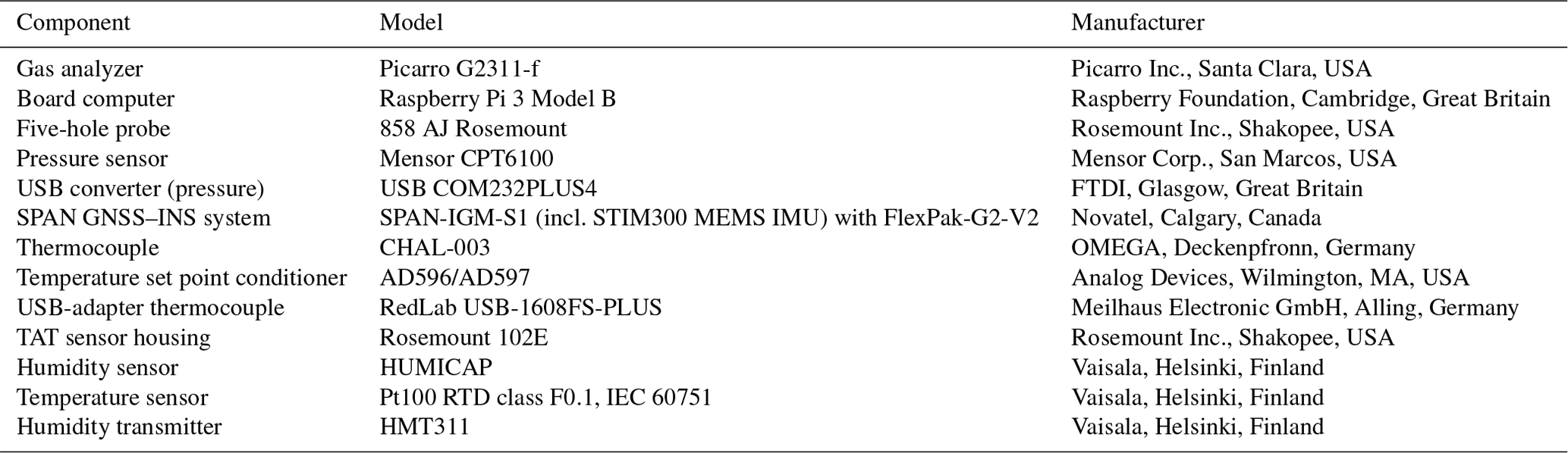
Table 2 Overview of the recorded variables, recording frequency, response rate (in brackets), measurement range, and the accuracy and the precision of the measurement. In most cases, measurement uncertainty and range were obtained from data sheets from the manufacturers (Picarro, Vaisala, Novatel, Mensor, Omega, Rosemount) and from Buetow (2018), Lehmann (2022), National Institute for Standards and Technology (1999), and Yang et al. (2016). The precision of recorded variables from the INS–GNSS (indicated with ^*) was obtained from on-ground measurements on 4 May 2022 in Lüsse, Germany, where the aircraft remained stationary for ca. 1 h.

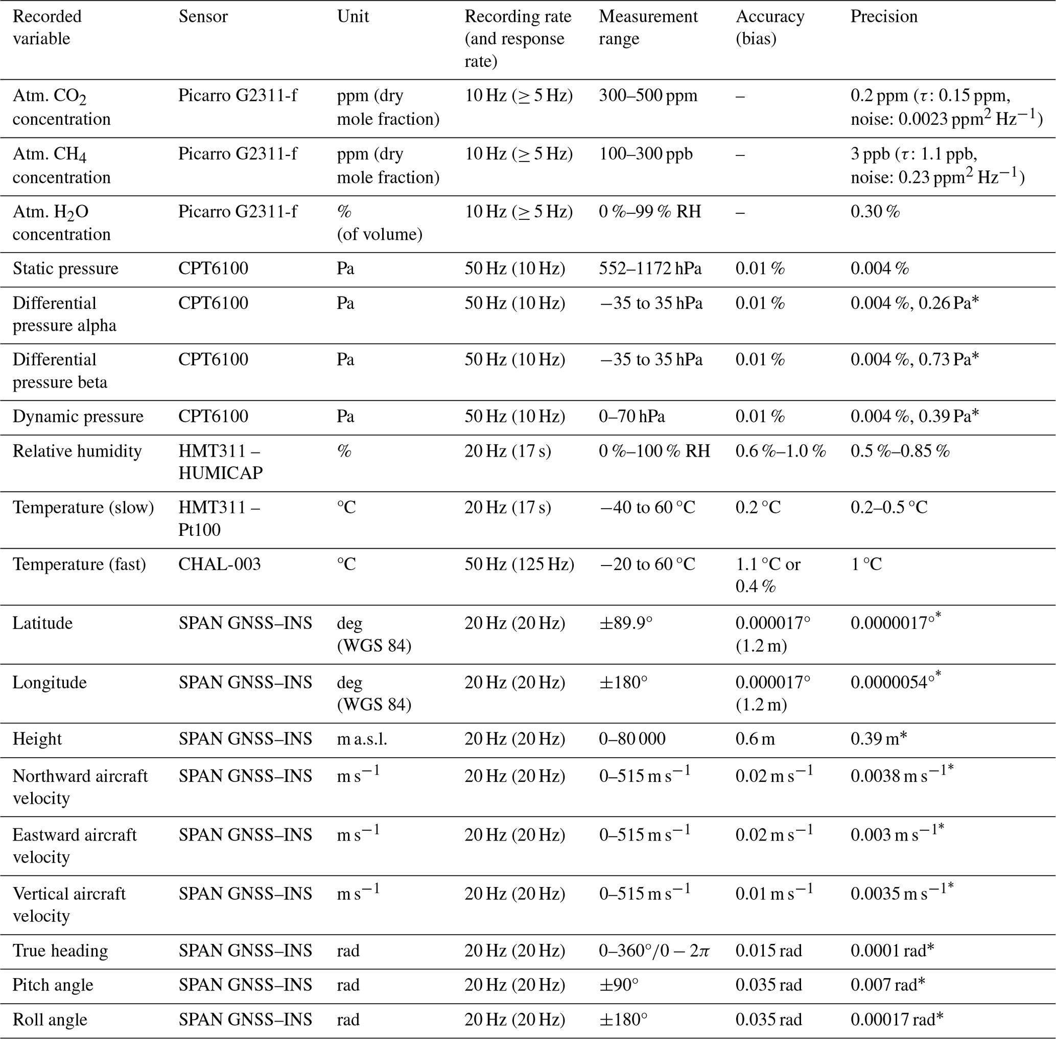
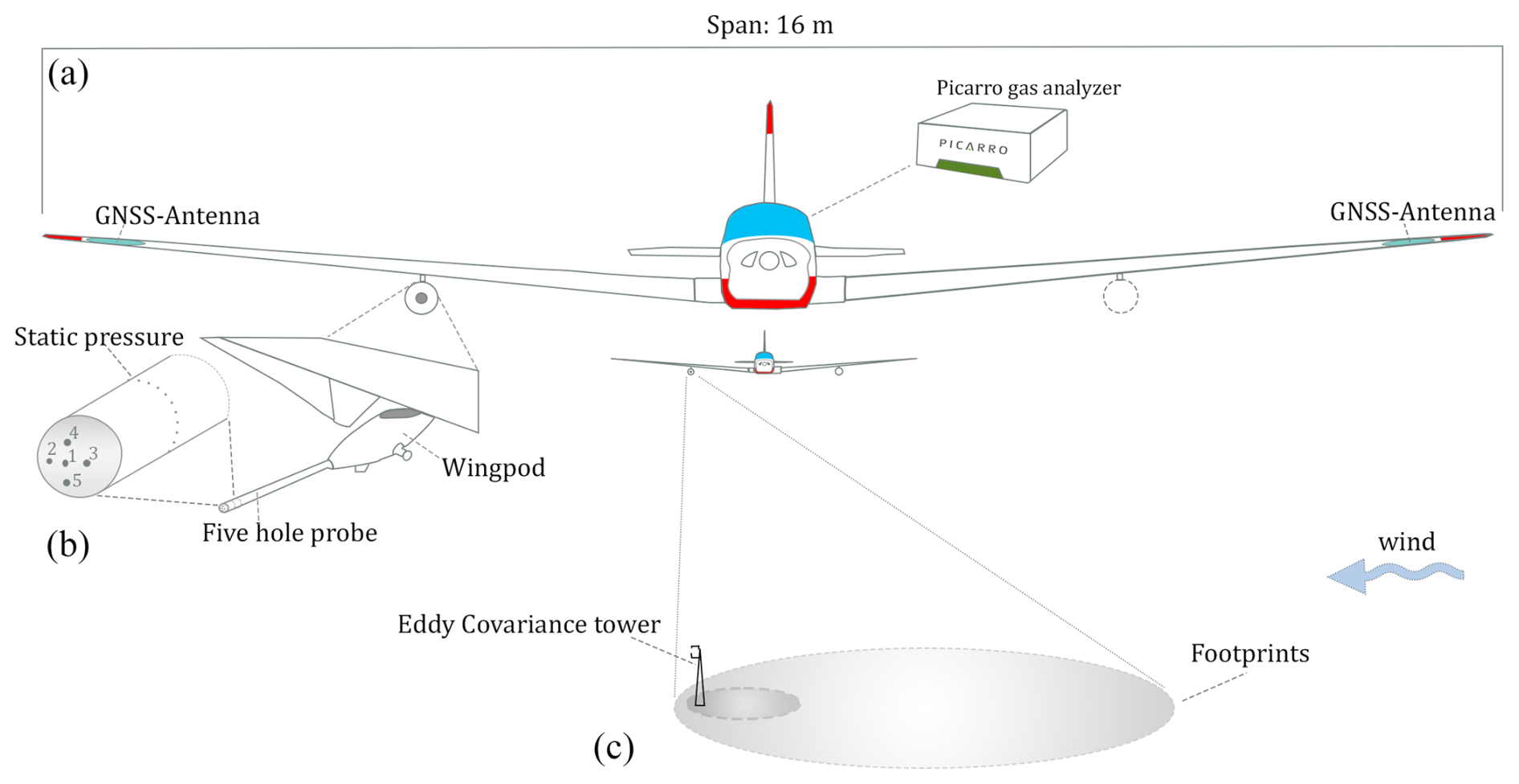
Figure 1 Setup of the ASK-16 eddy covariance measurement platform showing (a) the general measurement setup, (b) the five-hole probe, and (c) a schematic representation of the footprint of such an airborne measurement platform in comparison to an eddy covariance tower. Keep in mind that the real difference in footprint magnitude depends on the measurement heights of the tower and the aircraft. More details about the instrumentation aboard the ASK-16 are provided in Table 1.

For airborne eddy covariance campaigns, the motorized glider is equipped with sensors to obtain high-frequency fluctuations in wind, CO₂, CH₄, temperature, and water vapor (Table 1 and Fig. 1). A Picarro G2311-f gas analyzer (Picarro Inc., Santa Clara, USA) is installed in the cabin of the ASK-16 to measure high-frequency gas concentrations (10 Hz). On the front of the wingpod, an 858 AJ Rosemount five-hole probe (858 AJ, Rosemount Inc., Shakopee, USA) is mounted, which is connected to four CPT6100 pressure transducers (Mensor Corp., San Marcos, USA) located within the pod. The distance between the inlet of the tube and the gas analyzer and the five-hole probe was small (< 0.5 m). The tube was ca. 6 m long, had a flow rate of ca. 5.8 standard liters per minute, and had an inner diameter of ca. 0.04 m. Based on these characteristics, the transport time of the gas between the inlet tube and the G2311-f gas analyzer was ca. 0.8 s. Behind the pressure transducers, a SPAN-IGM-S1 system (Novatel, Calgary, Canada) is installed that integrates a combined GNSS–INS solution. Global Navigation Satellite Systems (GNSS) antennas are installed in the wings of the motorized glider, which are connected with the IMU and the satellite receiver. To increase the GNSS position and angle accuracy, a second GPS receiver was connected to the GNSS–INS system (FlexPak G2-V2; Novatel, Calgary, Canada). Additionally, the wingpod contains a Pt100 RTD temperature sensor (class F0.1 IEC 60751, Vaisala, Helsinki, Finland) and HUMICAP humidity sensor (Vaisala, Helsinki, Finland), which are connected to a HMT311 temperature and humidity transmitter (Vaisala, Helsinki, Finland). In 2019, a CHAL-003 thermocouple temperature sensor (OMEGA, Deckenpfronn, Germany) was additionally installed on the outside of the wingpod, close to the five-hole probe to measure high-frequency temperature and calculate sensible heat fluxes. All time stamps of the sensor blocks are synchronized to the inertial navigation system.

All sensors in the wingpod are connected to a Raspberry Pi 3 (Model B; Raspberry Pi Foundation, Cambridge, United Kingdom) through Universal Serial Bus (USB) interfaces (see Table 1). Data logging is managed with hgpstools (https://bitbucket.org/haukex/hgpstools, last access: 10 January 2025, developed by Hauke Dämpfling, Leibniz Institute of Freshwater Ecology and Inland Fisheries (IGB), Berlin, Germany), an open-source software package written in Perl. The software manages the communication between the single board computer (Raspberry Pi) and the sensors. Table 2 provides a full list of all recorded variables, their measurement frequency, and their measurement uncertainty.

2.2 Data processing: eddy4R and PyWingpod

To process the data and calculate wind vectors and turbulent fluxes, two software packages were used in this study: eddy4R (Metzger et al., 2017) and PyWingpod. Figure 2 shows the entire data processing procedure for the ASK-16 flight data: from raw data to wind vector data to calculated flux output. It shows which processing steps are performed by which software package and what output data are generated. The structure of this paper follows the processing steps visualized in Fig. 2.

First, the data were processed with the PyWingpod toolbox, developed in Python (version > 3.7) by the German Research Centre for Geosciences (GeoForschungsZentrum Potsdam) and the Free University of Berlin (Freie Universität Berlin) to specifically process the wingpod data of the ASK-16. This software package includes different libraries created for the preprocessing and calibration of the wingpod data. It also incorporates functions to calculate the final wind vector and additional meteorological variables, which are partially based on functions in EGADS, version 0.8.9 (EUFAR General Airborne Data-processing Software), a Python-based toolbox for processing airborne atmospheric data which can be accessed via GitHub (https://github.com/EUFAR/egads, last access: 10 January 2025). The software package PyWingpod provides several additional functions to visualize the data during these different data processing steps and can generate additional output (e.g., figures, tables, .kml files, and shapefiles), which can be used for further data exploration.

Afterwards the wind vector output and wingpod data were merged with Picarro data and further processed in eddy4R (Metzger et al., 2017) to calculate fluxes and footprints. eddy4R consists of a family of EC code packages (currently eddy4R.base, eddy4R.qaqc, eddy4R.stor, eddy4R.erf, eddy4R.turb, and eddy4R.ucrt), each consisting of a set of functions that have been developed in the open-source R language (R Core Team, 2021). Using a combination of functions from the eddy4R universe, wavelet-based fluxes, Reynolds fluxes, and footprints were calculated, and a quality and uncertainty assessment of the fluxes was performed (Fig. 2 – blue region).

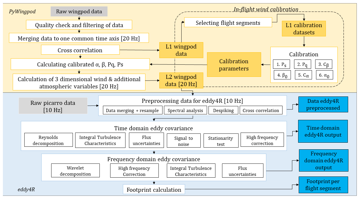
Figure 2 Workflow ASK-16 platform for processing airborne eddy covariance data. The yellow section describes workflows performed in the Python toolbox PyWingpod. The blue region shows the workflow as performed in eddy4R (Metzger et al., 2017). Colored boxes display input/output of by the software: gray boxes represent raw input; yellow boxes represent output created by PyWingpod, whereas blue boxes present output created by eddy4R packages.

2.3 Wind vector calculation

One of the two main components of the eddy covariance technique is the measurement of the turbulent wind vector at high frequency (Vellinga et al., 2013), for which we used the calculations as described in detail by Lenschow (1986) and Lenschow and Spyers-Duran (1989). As the wind vector is measured from a moving platform (motorized glider), the wind vector (V_wind) is calculated as a difference between the true airspeed (V_tas; measured by the five-hole probe) and the groundspeed (V_gs; measured by the GNSS–INS system) according to the following equation:

$$\begin{array}{}\text{(1)}& V_{\mathrm{wind}}=V_{\mathrm{gs}}-V_{\mathrm{tas}}+\mathrm{\Omega }\times L.\end{array}$$

The displacement term Ω×L accounts for the displacement between the INS–GNSS and the five-hole probe, where L describes the lever arm length (distance between accelerometer and five-hole probe, here 0.85 m), and Ω represents the angular velocities of the motorized glider (Mallaun et al., 2015). A more detailed description of the wind calculation procedure can be found in Lenschow and Spyers-Duran (1989).

2.4 Measurement calibration

To reduce the aerodynamic position errors of the five-hole probe (alignment of the probe relative to the flow field and the position in the airflow around wings and fuselage), several calibration flights were performed in order to increase the accuracy of the calculated three-dimensional (3D) wind vector. Calibration was performed on the static pressure (p_s), dynamic pressure (p_q), and the differential pressure measurements (p_α, alpha pressure; p_β, beta pressure) to improve V_tas. As you can see in the calibration equations below, p_α and p_q are used for the calculation of the angle of attack (α; see Eq. 2), and p_β and p_q are used for the calculation of the sideslip angle (β; see Eq. 3):

$$\begin{array}{}\text{(2)}& \mathit{\alpha }={\displaystyle \frac{p_{\mathit{\alpha }}}{C_{\mathit{\alpha }}\cdot p_q}}-{\mathit{\alpha }}_{\mathrm{0}}.\end{array}$$

Here, C_α and α₀ are the calibration parameters, which describe the sensitivity to the inverse slope of p_α and the offset of the angle of attack.

$$\begin{array}{}\text{(3)}& \mathit{\beta }={\displaystyle \frac{p_{\mathit{\beta }}}{C_{\mathit{\beta }}\cdot p_q}}-{\mathit{\beta }}_{\mathrm{0}}\end{array}$$

In this equation, C_β describes the inverse slope of p_β in the calibration equation and β₀ the offset.

The calibration of the pressure measurements is an important procedure for airborne eddy covariance measurements, as the calculated wind is highly sensitive to input uncertainties (see, e.g., Metzger et al., 2011). In this paper, we focus on describing the on-ground and in-flight calibration procedures applied for ASK-16 wingpod data specifically. Detailed descriptions of all available state-of-the-art in-flight calibration procedures are, for example, provided by Drüe and Heinemann (2013), Vellinga et al. (2013), and Mallaun et al. (2015).

2.4.1 Temporal and spatial alignment of the wingpod data

Time lags between sensors can be caused by differences in processing speeds of different sensors (Drüe and Heinemann, 2013). Although these lags are mostly small (< 1 s; Drüe and Heinemann, 2013), such lags need to be detected, as time alignment is crucial to ensure an accurate wind and reliable turbulent fluxes. Therefore, potential time lags between measurement data recorded by different devices were assessed before other calibration procedures were performed. To assess the time alignment of the sensors, the assumption was made that measurements from the same measurement group (A/D converter or sensor block) should have the same lag, which is similar to the approach used by Drüe and Heinemann (2013). In our case, we assessed the time lags for four different sensor groups: pressure sensors (block 1), INS–GNSS sensors (block 2), temperature sensors (block 3), and all HMT Vaisala sensors (block 4). While performing cross-correlation analysis for the different sensor groups, no clear lags were observed between any of the wingpod's sensor groups. Therefore, no time shifts were applied to any of the four sensor groups within the wingpod. Temporal alignment of the wingpod data and the Picarro data is performed at a later stage in the data processing using eddy4R (see Fig. 2). Generally, the lag between the gas analyzers and the wind measurements is corrected using a high-pass-filtered cross-correlation technique as detailed in Sect. 2.5 (Metzger et al., 2017; Hartmann et al., 2018). Spatial alignment between the INS–GNSS and the five-hole probe is also assessed during the pressure angle calibration. We used the offset of β₀ and α₀ to describe the offset in the alignment of pitch and yaw angles. The alignment of the roll angle between the INS–GNSS and the five-hole probe was not assessed and set to 0, similar to Vellinga et al. (2013).

2.4.2 On-ground calibration of the wingpod data

Before in-flight calibration maneuvers were analyzed, on-ground calibration was performed to correct for potential offsets in the pressure sensor data. Such offsets can affect the final wind vector and therefore need to be determined. Before the start of a measurement flight, the wind inflow into the pressure holes was covered by placing a glass fiber composite non-airtight cap onto the five-hole probe. The on-ground pressure data for this wind-free period were analyzed afterwards to characterize the bias in dynamic pressure (q_i), α pressure (p_α), and β pressure (p_β). In this setup, the static pressure offset could not be assessed. For the available datasets, we mostly used a 30 min pressure record to determine the offsets. If the duration of the on-ground and wind-free period was shorter, we used the available time frame with stable measurements, with the restriction of having at least 10 min of data. In our case, the pressure offsets were very small and ranged between 1 and 10 Pa for the different pressure measurements.

2.4.3 In-flight calibration maneuvers

In our study we used five in-flight calibration maneuvers (reverse heading, pitching, yawing, and speed maneuvers and wind squares) for the calibration of pressure measurements (q_i, q_s, q_α, and q_β), the corresponding α and β angles (see Sect. 2.4), and for the evaluation of the calibration procedure (Fig. 3). Each individual in-flight calibration procedure mainly focuses on the calibration of a single variable, while trying to rule out or minimize the effect of external factors on that specific calibration parameter.

During a speed maneuver (Fig. 3a), the speed of the aircraft is first slowly increased (acceleration segment) and afterwards slowly decreased (deceleration segment) at a relatively constant altitude. This procedure is repeated multiple times to study the effect of speed variations on the different pressure measurements of the five-hole probe (α, P_q, and P_s). During a pitching maneuver (Fig. 3b), the nose of the aircraft moves sinusoidal upwards and downwards by the deflection of the aircraft's elevator. The airplane turns around its lateral axis, altering the pitch angle (θ) of the aircraft, and induces a change in the angle of attack (α). This maneuver is used for the calibration of α and uses the concept that pitch oscillations should not significantly affect the vertical wind measurement (w).

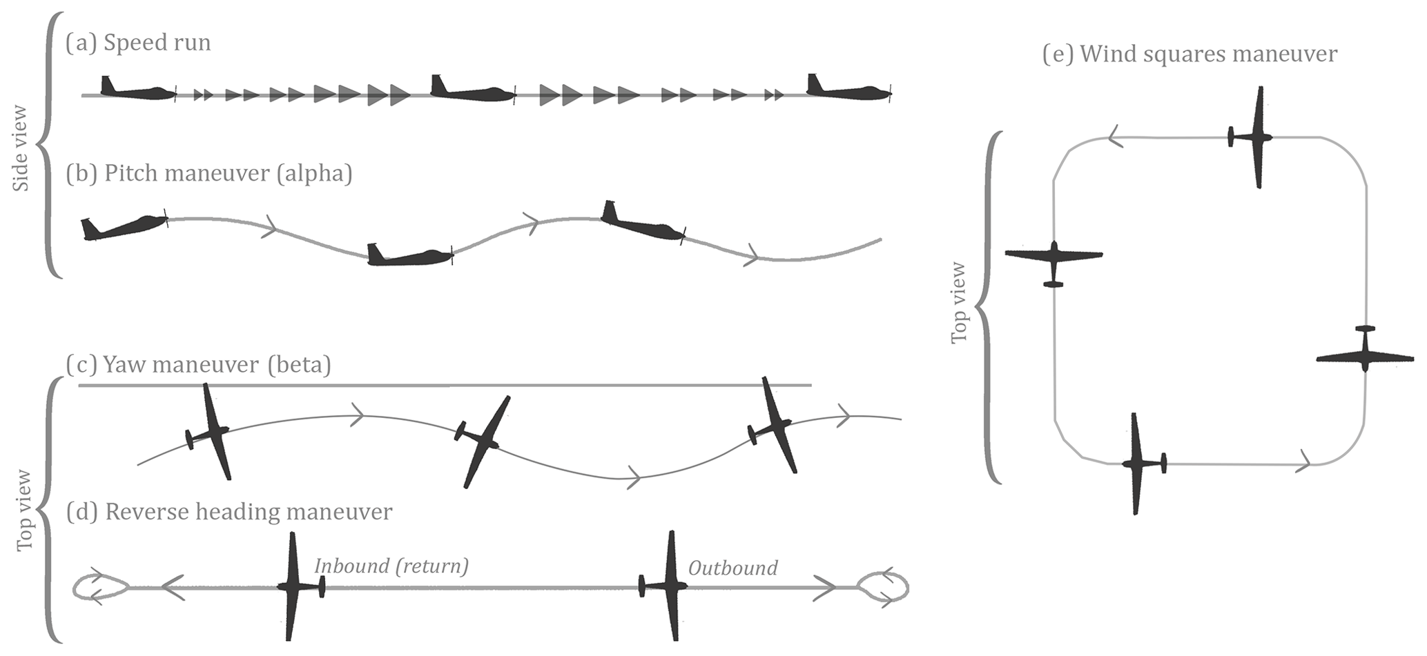
Figure 3 Schematic illustration of flight maneuvers performed with the ASK-16 to calibrate the pressure measurements of the five-hole probe, including speed runs (a), jaw and pitch maneuvers (b, c), reverse heading maneuvers (d), and wind squares maneuvers (e).

Yawing maneuvers (Fig. 3c), on the other hand, are performed to calibrate the sideslip angle (β). During a yawing maneuver, the aircraft is rotated harmonically sinusoidal around its vertical axis (heading; nose moving left/right) by engaging the rudder and aileron(s). The aircraft is kept at a (more or less) constant altitude. To calibrate for β, we use the assumption that the horizontal components of the wind (u, v) should not be affected by yaw maneuvers. Reverse heading maneuvers (Fig. 3d), also called return track flights (Hartmann et al., 2018), were performed for the calibration of the dynamic pressure (q_i) and β and α angles. The aim of this maneuver is to fly two times through a very similar air mass, while keeping the time difference between the outbound and return flight as small as possible. Wind squares (Fig. 3e) are box-shaped flight patterns, where the airplane flies a straight track four times, separated by 90° turns. During this maneuver, altitude and airspeed are kept as constant as possible. In our case, the maneuver was used as a second check to assess the quality of the calibration procedure (see Sect. 2.6).

As several of the in-flight calibrations require the calculation of an a priori wind, the order of the calibration procedure can slightly affect the calibration outcome. Here, the order of the calibration was based in the first instance on a sensitivity analysis (Lehmann, 2022) starting with the two least sensitive parameters (here static pressure and dynamic pressure). Due to the difference in magnitude and importance of the wind components for airborne eddy covariance flux calculations, we furthermore first optimized the parameters related to the horizontal wind components (C_β and β₀) and then optimized the parameters that are directly connected to the vertical wind component (C_α and α₀), as proposed by Metzger et al. (2011). Although cross-dependences in the calibration procedure can be dealt with by iteratively optimizing the calibration (Metzger et al., 2011), this was not performed in our study. Here, we assume that the range and amount of calibration maneuvers will be sufficient to obtain suitable calibration parameters during different flight conditions.

Flight maneuver data were processed with the PyWingpod Python software package (Wiekenkamp et al., 2024b) to determine the calibration coefficients as described in the upcoming sections. In this study, no wind tunnel experiments were performed, but results from earlier studies (both wind tunnel experiments and in-flight calibrations) were used as a reference. As the wingpod of the ASK-16 was first installed in 2017 and re-installed in 2019, two calibration parameter sets were calculated for the static pressure, dynamic pressure, α, and β (calibration parameters for 2017–2018 and calibration parameters for 2019–2022).

2.4.4 Static pressure calibration

Although the static pressure measurement should represent that of a free airstream, the measured static pressure can be influenced by the flow around the aircraft, causing it to differ from the ambient static pressure. This pressure deviation is often referred to as static pressure defect (p_s,err) and needs to be defined to adjust the measured static pressure. Past research has shown that the static pressure defect depends on (1) the speed of the aircraft but also on (2) changes in the flow angles α and β (Bögel and Baumann, 1991; Drüe and Heinemann, 2013; Tjernström and Friehe, 1991). In this study, the static pressure defect (p_s,err) is determined via speed runs (at relatively constant altitude) and yawing maneuvers, according to Kalogiros and Wang (2002). Speed maneuvers with varying p_α were used to assess the effect of the airplane on speed fluctuations (recorded in the dynamic pressure) and the effect of different α flow angles on the static pressure. Yaw maneuvers were used to assess the effects of different β flow angles on the static pressure. Data from each single maneuver were used to fit the following polynomial equation:

$$\begin{array}{}\text{(4)}& p_{\mathrm{s},\mathrm{err}}=\left(a_{\mathrm{1}}\times p_q\right)+\left(a_{\mathrm{2}}\times p_q\times p_{\mathit{\alpha }}^{\mathrm{2}}\right)+\left(a_{\mathrm{3}}\times p_q\times p_{\mathit{\beta }}^{\mathrm{2}}\right),\end{array}$$

where p_q represents the dynamic pressure, a₁–a₃ are the calibration parameters, and p_β and p_α are the differential pressure measurements. Speed maneuvers were used to determine a₁ and a₂, and yaw maneuvers were used to calibrate a₃. During the determination of calibration parameters for each single maneuver, the calibration data were offset-corrected (resulting in an absolute offset of 0). To exclude the influence of following calibrations (C_α, C_β, α₀, and β₀) on the adjusted pressure, possible influences of sideslip and angle of attack on the static pressure were accounted for using the differential pressure measurements p_α and p_β. To rule out the influence of altitude fluctuations during the speed maneuvers, the static pressure was first normalized by altitude. Here, the barometric pressure was calculated for the assigned measurement height. Afterwards, a polynomial function was fitted between the normalized static pressure (independent variable) and one or multiple dependent variables (p_α, p_β, and p_q), resulting in a function that can be used to correct the measured static and dynamic pressure.

2.4.5 Dynamic pressure calibration

The dynamic pressure calibration was performed in two steps. First, the dynamic pressure was adjusted by adding the static pressure defect (Sect. 2.4.4, Eq. 4) to the dynamic pressure measurement. Afterwards, we used the dynamic pressure calibration method as proposed by Hartmann et al. (2018), using the assumption that the average groundspeed over an outbound (vector index 1) and return flight (vector index 2) is equal to the average true airspeed:

$$\begin{array}{}\text{(5)}& {\displaystyle \frac{\mathrm{1}}{\mathrm{2}}}\times \left({\displaystyle \frac{v_{\mathrm{gs},\mathrm{1}}}{\cos \left(\mathit{\gamma }\right)}}+{\displaystyle \frac{v_{\mathrm{gs},\mathrm{2}}}{\cos \left(\mathit{\gamma }\right)}}\right)={\displaystyle \frac{\mathrm{1}}{\mathrm{2}}}\times \left(\left|v_{\mathrm{tas},\mathrm{1}}+v_{\mathrm{tas},\mathrm{2}}\right|\right)=v_{\mathrm{ref}}.\end{array}$$

Based on the magnitude of the drift (and the difference between χ, the true track, and θ, the true heading ($\mathit{\chi }-\mathit{\theta }=\mathit{\gamma }$)), we needed to include cos (γ) in our equation (Eq. 5). Afterwards, the reference undisturbed dynamic pressure (p_q.ref) was determined using the following equation:

$$\begin{array}{}\text{(6)}& p_{q.\mathrm{ref}}={\displaystyle \frac{\frac{\mathrm{1}}{\mathrm{2}}\times \mathrm{1}}{\mathit{\rho }\times {v_{\mathrm{ref}}}^{\mathrm{2}}}}.\end{array}$$

Next, we plotted the average measured dynamic pressure (p_q.i) against the reference undisturbed pressure (p_q.ref) to calculate a correction factor (c_q):

$$\begin{array}{}\text{(7)}& p_{q.\mathrm{ref}}=c_q\times p_{q.i}.\end{array}$$

This calculated correction factor was then used to adjust the measured dynamic pressure.

2.4.6 C_β and β₀ calibration

Similar to the static and dynamic pressure, the angle of attack and sideslip angle are affected by pressure field deformations around the aircraft, which can cause deviations between the measured and the real α and β angles (Drüe and Heinemann, 2013). To correct for these deviations, the sideslip angle was calibrated using Eq. (3). To determine C_β, yawing maneuvers were used, which are commonly applied for such calibration (e.g., Bögel and Baumann, 1991; Drüe and Heinemann, 2013; Mallaun et al., 2015; Williams and Marcotte, 2000). In a first step, the wind vector is calculated for a yawing maneuver. Afterwards, the sum of the standard deviation in the horizontal wind components u and v is calculated. Iteratively, this summed standard deviation is optimized using the Nelder–Mead optimization algorithm in SciPy (Virtanen et al., 2020).

To determine β₀ (the offset of β), we used a set of outbound and return flights (reverse heading maneuvers). Here, the difference between the average horizontal wind components (u and v) was iteratively minimized for each maneuver (Williams and Marcotte, 2000; Drüe and Heinemann, 2013) using the Nelder–Mead optimization method in SciPy (Virtanen et al., 2020). As local flight conditions and the selection of the exact flight segments can affect the outcome of the β₀ optimization, the mean β₀ was calculated from a large set of reverse heading maneuvers.

2.4.7 C_α and α₀ calibration

The calibration of the angle of attack α was performed using a variety of calibration methods. Similar to the correction of the sideslip angle, the angle of attack can be calibrated using Eq. (2). First C_α is determined using flight data from slow pitching maneuvers. For these flight maneuvers, first the vertical wind speed was calculated, using an offset of 0 (α₀) and the manufacturer-supplied correction factor of 0.079 $[\mathrm{1}/\mathit{°}]$ as provided by Rosemount (Drüe and Heinemann, 2013). Here, we assumed that the obtained variability in vertical wind speed was mainly caused by the movement of the airplane and should be minimized (Bögel and Baumann, 1991; Mallaun et al., 2015). Therefore, we optimize the sensitivity parameter C_α iteratively by minimizing the standard deviation of the vertical wind (w) with the Nelder–Mead optimization algorithm in SciPy (Virtanen et al., 2020).

Afterwards, we used flight data from straight level flights with small speed variations to obtain a calibration parameter for α₀. This second calibration procedure assumes that if we fly long enough over a straight track, the average vertical wind component should ideally reach 0. Therefore, we first calculate the average wind speed over the flight segment without offset and then iteratively optimize α₀ by minimizing the absolute average vertical wind component.

As an alternative approach, data from speed maneuvers and/or reverse heading maneuvers can be used to calibrate α, as proposed by Hartmann et al. (2018). For this calibration procedure, we used the fact that, without aircraft pressure field deformations, the angle of attack equals the pitch angle $(\frac{p_{\mathit{\alpha }}}{p_q}=\mathit{\theta })$. This is only valid during straight level flights and for fixed-wing aircraft, where α varies with airspeed. Similar to Hartmann et al. (2018), speed maneuver data were first used to assign the relationship between $\frac{p_{\mathit{\alpha }}}{p_q}$ and θ, while accounting for vertical movement of the plane (w_p). Based on the obtained relationship, C_α and α₀ were calculated. In a second step, we selected flight sections where the vertical movement of the plane was less than 1.5 m s⁻¹.

2.5 Flux and footprint calculation

After the wind data were calibrated and the 3D wind vector was calculated (20 Hz), these data were merged with data from the Picarro gas analyzer (10 Hz). In this case, a nearest-neighbor interpolation was applied to the wind and Picarro data to bring both datasets on a common time axis with a resolution of 10 Hz and retain the amplitude of the original measurements. Subsequently, outliers were detected in the different data products using a nonlinear median filter algorithm with a window of seven points (N = 3) according to Brock (1986) and Starkenburg et al. (2016). Afterwards, two types of flight segments are extracted from the combined dataset: (1) vertical flight segments and (2) straight level segments (legs). Data from vertical flight segments (potential temperature, relative humidity, and CH₄ and CO₂ concentrations) are used to infer the thickness of the atmospheric boundary layer. Straight horizontal flight segments (legs) are further processed to calculate surface fluxes.

Data from flight legs were further used for flux processing with eddy4R (Metzger et al., 2017). Lag times were obtained for every flight leg by performing a high-pass-filtered cross-correlation between w^′ and the gas concentrations (H₂O, CO₂, and CH₄) as proposed in Hartmann et al. (2018). CO₂ and CH₄ concentrations were afterwards shifted according to the median lag of a particular flight. As the latency of H₂O can be variable within a single flight, no median lag for an entire flight was applied. Instead, individual lags were assigned for each individual flight leg of a specific flight. No lag correction was applied to the temperature data, as no clear lag could be determined between w^′ and T^′.

The flux calculation for each leg was performed with the eddy4R (Metzger et al., 2017) packages according to Metzger et al. (2012, 2013), following the workflow as shown in Fig. 2. Although airborne fluxes are also calculated using a time-domain-based approach, the focus here is on the fluxes calculated with a time–frequency-domain-based (wavelet-based) approach. This wavelet-based approach is explained in detail by Metzger et al. (2013). In short, a continuous wavelet transform approximation according to Torrence and Compo (1998) was performed for each individual leg, for all relevant variables (u, w, T, H₂O, CO₂, and CH₄) using the Morlet wavelet as a mother wavelet. Afterwards, a cross-scalogram was calculated using the measured vertical wind and a second scalar (here T, H₂O, CO₂, and CH₄). Next, the integral of the cross-scalogram was calculated at the original resolution and for each flux segment using a given window size. Based on the flight altitude of the ASK-16 (ca. 150–250 m above the surface), fluxes were calculated every 200 m with an overlapping moving window of 2000 m. Using a time–frequency resolved version of the eddy covariance methods results in a higher spatial discretization where multiple flux segments are calculated for a single leg. Using wavelets, contributions from the longer wavelengths (large eddies) are incorporated in these flux segments. Instead of obtaining only a single flux estimation per flight leg, we can now obtain an entire transect of fluxes.

The step size and window length used in our flux calculation were chosen based on previous work by Metzger et al. (2012, 2013), taking into account the altitude of the aircraft, atmospheric mixing, the characteristic length scales, and resolution of surface features. The window size for flux calculation, set to 2000 m, is designed to balance the trade-off between random error (which decreases with larger window sizes) and resolution (which increases with smaller windows). As shown in Metzger et al. (2013), longer windows reduce random flux error due to the inverse proportionality between random error and the square root of the averaging length (Lenschow and Stankov, 1986). Additional details on the rationale behind the selected window and step sizes are provided in Metzger et al. (2013), which discusses the balance between resolution and error in flux calculations over heterogeneous landscapes.

Although this approach results in fluxes with largely overlapping samples, the individual overlapping samples are still very valuable, because they preserve high spatial resolution. This is critical for capturing sharp transitions in fluxes (e.g., from land to lake) and for reducing random noise in turbulent atmospheric conditions. Additionally, wavelet-based flux calculation benefits from this approach, as it allows for multi-scale analysis and better characterization of spatial heterogeneity, compared to traditional Reynolds-averaging methods that smooth out small-scale variations.

Footprints were calculated by combining the Kljun et al. (2004) along-wind footprint with a Gaussian crosswind distribution function as described in Metzger et al. (2012). This combination makes the footprint formulation more applicable for higher altitudes and thus for airborne eddy covariance. Inputs for the calculated footprint function include (1) the measured friction velocity, (2) measurement altitude, (3) the standard deviation of the lateral and vertical wind (σv, σw), (4) the boundary layer height, and (5) the calculated roughness length according to Högström (1988). After the calculation of the footprints, single segment footprints, leg-integrated footprints, and flux footprints (flux × footprint) were calculated. This will enable us to create follow-up products, such a flux topographies (e.g., Kohnert et al., 2017) or integration with earth observations to regional flux maps through physics-guided artificial intelligence (e.g., Metzger et al., 2013; Serafimovich et al., 2018; Vaughan et al., 2021).

2.6 Measurement accuracy and quality assessment

To obtain information about the quality and uncertainty of the measurements during the flights, several analyses were performed for individual flights and single flight legs. Airborne turbulent fluxes that are obtained by using the eddy covariance method are only valid under (1) steady-state conditions with (2) developed turbulence (Foken, 2017). To evaluate the flight conditions, the integral turbulence characteristics were calculated and stationarity was assessed. Stationarity was assessed using (1) a trend analysis and (2) an internal instationarity analysis according to Foken and Wichura (1996) and Vickers and Mahrt (1997). Although wavelet-based fluxes (Morlet) are less sensitive to instationarities (see, e.g., Schaller et al., 2017), we still use these characteristics as a quality measure for the calculated fluxes. For each flight segment, integral turbulence characteristics were calculated for measured and modeled u, w, and u^* according Thomas and Foken (2002). Leg segments that surpassed the threshold above 100 % were flagged.

Besides flight conditions, measurement errors and flux detection limit are important, as they provide information about the potential and limitations of the measurement platform. Flux detection limits were calculated for each single flight leg by performing a random flux uncertainty estimation according to Billesbach (2011). Here, a random flux uncertainty estimation is used, where fluxes are recalculated for randomly shifted time series to assess the flux detection limits. Systematic and random statistical errors were calculated according to Mann and Lenschow (1994) and Lenschow and Stankov (1986). Spectral characteristics of the individual measured gases and wind components were assessed by looking at the spectra of the wind components, fast temperature, and measured gases, as performed, e.g., by Hartmann et al. (2018), Metzger et al. (2011), and Wolfe et al. (2018).

The use of 2 km integration windows with 200 m step size may introduce some autocorrelation due to 90 % overlapping samples, which could artificially reduce ensemble random errors:

$$\text{Error}={\displaystyle \frac{\mathit{\sigma }}{\sqrt{N}}},$$

where σ is the standard deviation of the random error in individual samples and N is the number of independent samples. We have accounted for this by recognizing that overlapping samples are autocorrelated, and the effective sample size N_eff is reduced accordingly, following the formula

$$N_{\mathrm{eff}}={\displaystyle \frac{N}{\mathrm{1}+\mathrm{2}{\sum }_{k=\mathrm{1}}^K\mathit{\rho }\left(k\right)}}.$$

Here, ρ(k) is the autocorrelation function of the sample with lag k, and K is the maximum lag where significant autocorrelation exists. Using N_eff in place of N corrects the ensemble random error to reflect the increased autocorrelation between samples.

3 Results and discussion

3.1 Wind calibration results

In this study, the calibration of the static and dynamic pressure, as well as sideslip angle and angle of attack, was performed following the calibration scheme in Fig. 2, as described in detail in the methodology of this paper. For the calibration of all pressure-sensor-related calibration parameters, pitching maneuvers, yawing maneuvers, reverse heading maneuvers, and speed maneuvers were used (see Sect. 2.4.3–2.4.7). Information about the meteorological conditions during these flight maneuvers is provided in Sect. S1 in the Supplement: “Flight Maneuver Information”. Whereas metadata and calibration results from single calibrations are provided in Sect. S1, median calibration values and standard deviations that were assigned to the calibration periods 2017/2018 and 2019/2022 are given in Table 3. The description and discussion of the calibration results follow the order of calibration.

Table 3 Overview of obtained calibration parameters for the different monitoring periods (2017–2018 and 2019–2022) and their uncertainty (described by standard deviation σ of all obtained parameters obtained during the specific flight period). Final calibration parameters are described here by the median of all parameters that were obtained for the particular flight period (see Tables S1–S5 and Sect. S1). Values in brackets (C_α and α₀) present the calibration parameters obtained from the speed runs (see Fig. 8 and Sect. 3.1.4).

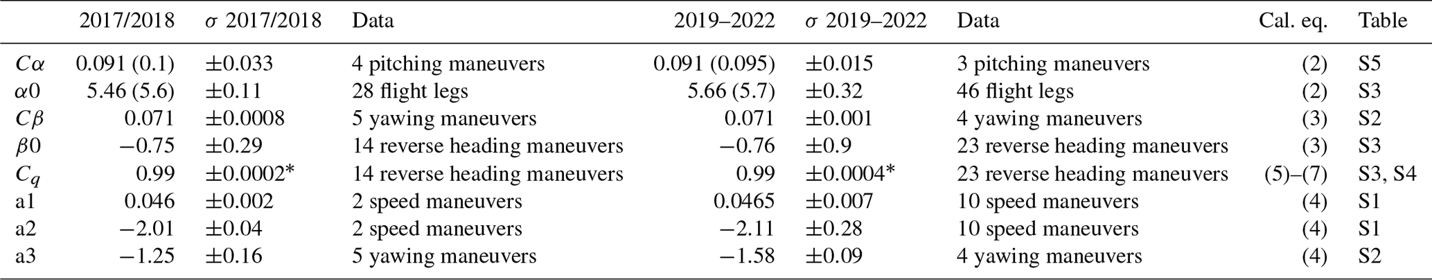
^* Standard deviations of C_q calibrations were based on the regression between the average q_i and q_ref values of reverse heading maneuvers as shown in Fig. 5.

3.1.1 Static pressure

The static pressure defect was assessed using data from 12 speed runs and nine yawing maneuvers that were performed over northern Germany between 2017 and 2022 (for more details, see Sect. S1 and Tables S1 and S2 in the Supplement), of which most speed runs were performed in 2019. Overall, external factors that could affect the calibration were relatively small and likely did not have a large effect on the determination of the static pressure defect. In most cases, speed runs were performed at an altitude of approximately 1000–1100 m a.s.l.; the maximum change in groundspeed during the speed maneuvers was approximately 21 m s⁻¹ (median over all speed runs), and the average vertical wind (w) was close to 0 (see Table S1). Yawing maneuvers were performed at an altitude ranging between 608 and 2602 m, and most maneuvers had an average vertical wind speed close to 0 m s⁻¹ (see Table S2).

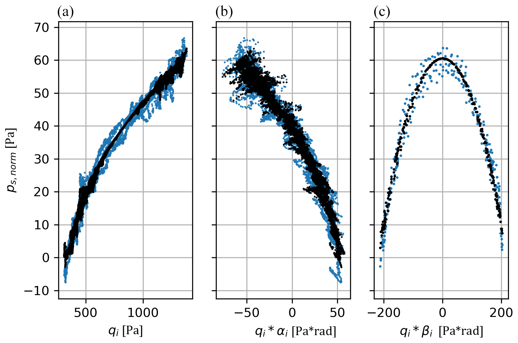
Figure 4 Example of the static pressure (p_s) calibration procedure for a calibration flight on 7 June 2018. A polynomial fit is calculated for the relationship between the altitude-normalized static pressure and (a) the indicated dynamic pressure (pq_i), (b) α_i, and (c) β_i, resulting in the following function: p_s,norm = $\mathrm{0.048}\times p_q-\mathrm{1.98}\times p_q\times {\mathit{\alpha }}_i^{\mathrm{2}}-\mathrm{1.25}\times p_q\times {\mathit{\beta }}_i^{\mathrm{2}}$. The blue dots in the figure present the measured data, and the black dots represent the fitted relationship (polynomial function).

In general, the static pressure defect could be well explained for all available maneuvers. Figure 4 shows an exemplary calibration for a speed and a yawing maneuver flown on 7 June 2018. Clearly, the static pressure defect could be explained by the variability in dynamic pressure and pressure angles (coefficient of determination (r²) = 0.98 for the speed maneuver and 0.86 for the yawing maneuver). For all other maneuvers, the static pressure defect was also well explained by p_q, p_α and p_β, resulting in r² values ranging between 0.91 and 0.99 for all speed maneuvers (median r² = 0.985) and between 0.71 and 0.98 for all yawing maneuvers (median r² = 0.97).

3.1.2 Dynamic pressure

The dynamic pressure was calibrated with 37 reverse heading maneuvers that were performed in Germany (DE) and the Czech Republic between 2017 and 2022 (for more details, see Sect. S1, Tables S3 and S4). In general, the average vertical wind was close to 0, and the conditions during the outbound and return flight were very similar (track length, flight time, wind speed, wind direction, wind vectors; see Table S4). Before the calibration parameters for the dynamic pressure were defined, we also checked if the average v_gs of each of the 37 flight pairs is similar to the average v_tas over both flight sections. This is crucial, as this is an important assumption for the calibration of the dynamic pressure according to Hartmann et al. (2018), specifically for Eq. (6). As shown in Fig. 5a, the relationship between v_gs and v_tas (where we account for γ, the difference between the true track and true heading) is located very close to the 1:1 line (y=1.02x). This means that flight conditions during both flight segments (outbound and return) were very similar, and dynamic pressure could be calibrated with Eq. (4).

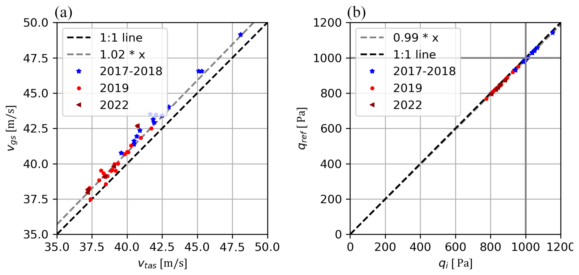
Figure 5 (a) Relationship between mean V_tas and V_gs for 37 reverse heading maneuvers colored by measurement year (2017–2018, 2019, and 2022). (b) Relationship between the average indicated dynamic pressure (q_i) and the reference dynamic pressure (for 37 reverse heading maneuvers; see Eqs. 5 and 6).

The results of the dynamic pressure calibration are presented in Fig. 5b. Clearly, the relationship between the average indicated dynamic pressure (q_i) and the average reference dynamic pressure (q_ref) of two overpasses is close to the 1:1 line (y=0.99x; see Table 3). These findings are different from Hartmann et al. (2018), who found a clear underestimation of the indicated dynamic pressure (c_q=1.165) as measured by the five-hole probe of the Polar 5 aircraft, showing that a correction of the dynamic pressure was required. Similar to Hartmann et al. (2018), we use the median average deviation from the regression line to estimate the accuracy of the calibration. Considering all 37 measurement flights, the median average deviation of the model residuals was 0.01 hPa, which is similar to the calibration accuracy obtained by Hartmann et al. (2018).

3.1.3 Sideslip angle

The in-flight calibration of β was performed using data from 9 yawing maneuvers and 37 reverse heading maneuvers that were recorded between 2017 and 2022 (for more details, see Sect. S1 and Tables S2–S4). Figure 6 shows an example of a sideslip angle calibration (C_β) for 21 September 2019. During the maneuver, five oscillations were performed, and the period of each oscillation was ca. 4.2 s (≈ 0.24 Hz). The amplitude of the maneuver was ca. 10° (crosswind), and the variability in the horizontal wind components after calibration was relatively small (σ(u) = 0.2 m s⁻¹; σ(v) = 0.16 m s⁻¹). This remaining variance of u and v followed the criterion proposed by Lenschow and Spyers-Duran (1989) and was below 10 % of the induced crosswind, suggesting a successful calibration.

Overall, the determination of C_β was successful, as the 10 % variance criterion according to Lenschow and Spyers-Duran (1989) was fulfilled for all nine yawing maneuvers. The overall standard deviation of u and v was small for all maneuvers (median σ(u) and σ(v) = 0.25 m s⁻¹), suggesting that the obtained calibration parameters can largely reduce the effects of heading changes on the horizontal wind vectors. The variability of the obtained C_β for the entire measurement period (2017–2022) was very small (σ(C_β) = 0.001), resulting in very similar calibration values for 2017/2018 (median C_β = 0.071; N = 5 maneuvers) and 2019/2022 (0.071; N = 4 maneuvers). This is in agreement with Hartmann et al. (2018), who already stated that C_β should not change over time (between different measurement campaigns).

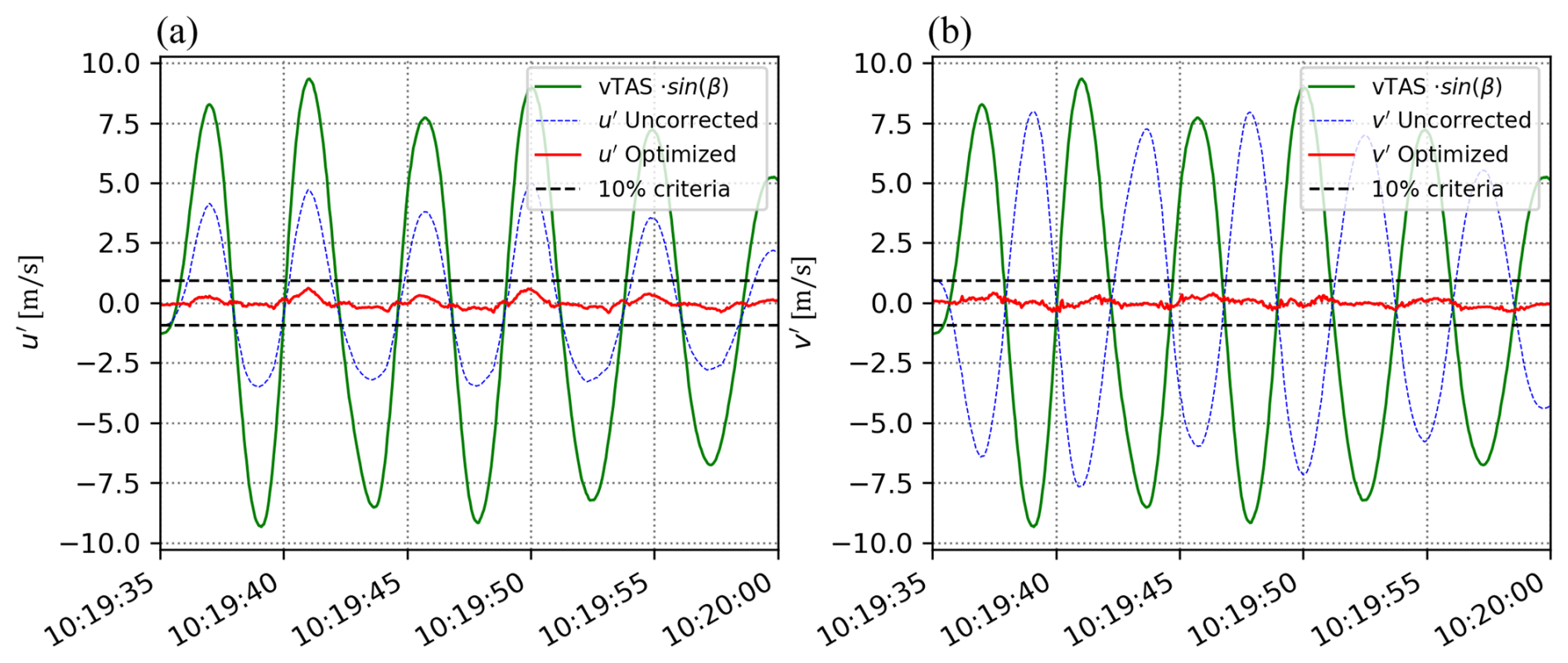
Figure 6 Results of sideslip angle calibration C_β for a yawing maneuver performed with the ASK-16 on 21 September 2019. During the determination of C_β, the standard deviation in u and v is optimized simultaneously. The blue line indicates u^′ (a) and v^′ (b) wind vectors with no consideration of C_β (C_β = 1); the red line shows the optimized u^′ and v^′ wind vectors (C_β = 0.071). Striped black lines indicate the maximum allowed deviation of u^′ and v^′ (10 % of the induced crosswind – in green) as proposed by Lenschow and Spyers-Duran (1989); σ_u and σ_v were 0.2 and 0.16 m s⁻¹, respectively.

The offset of β (β₀), on the other hand, is more likely to change after remounting the wingpod (Hartmann et al., 2018). The offset of β was determined with the 37 reverse heading maneuvers (see Sect. S1 and Table S4 for details on maneuver conditions). The variability in β₀ was the quite large (ranging from 0.49 up to −2.11), and the difference in mean u and v for the outbound and return flight ranged from small (0.01 m s⁻¹) to being substantial (1.98 m s⁻¹). These differences can also be caused by changes in local wind conditions and other flight conditions (e.g., altitude, difference in track). The differences in wind speed and wind direction are, on the other hand, acceptable, especially considering that it is impossible to have entirely similar atmospheric conditions during both legs. Overall, the average β₀ is very similar for both calibration periods (2017/2018: −0.75; 2019/2022: −0.76) and should provide a good offset value to reduce aircraft-related differences in average horizontal wind components as much as possible. As the given pairs contain quite different meteorological conditions, the applied parameterization should be applicable to a wide range of flight conditions (while fulfilling stationarity and integral turbulence characteristics criteria).

3.1.4 Angle of attack

Seven pitching maneuvers were performed between 2017 and 2022 to determine C_α (for more information see Sect. S1, Table S5). Figure 7 shows two examples of angle-of-attack calibrations for (a) a pitching maneuver performed on 18 July 2018 and (b) another maneuver that was performed on 7 June 2018. The amplitude of the vertical velocity of the aircraft during the pitching oscillations ranged from 7 m s⁻¹ (Fig. 7b) up to 15 m s⁻¹ (Fig. 7a), and the period of each oscillation was ca. 12.4–14.5 s. Similar to the yawing maneuvers, the variability in the vertical wind vector after calibration was relatively small (σ(w) = 0.17–0.27 m s⁻¹) compared to the amplitude of the vertical velocity of the aircraft (w_p = 15 m s⁻¹). The total oscillation was much smaller than the maximum allowed variation in w as proposed by Lenschow and Spyers-Duran (1989), showing that the calibration of the angle of attack was successful.

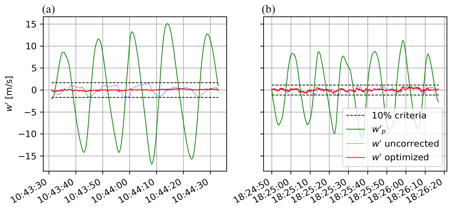
Figure 7 Results of the angle-of-attack calibration C_α for a pitching maneuver performed with the ASK-16 from (a) 18 July 2018 and (b) 7 June 2018. The blue line indicates vertical wind speed w^′ without any specific calibration (C_α = 1); the red line shows the optimized wind vector w^′ optimized (here C_α = 0.091 in panel a and 0.093 in panel b). During the determination of C_α, the standard deviation of w^′ is optimized. The mean vertical wind was subtracted from the measurement to better visualize the residual error in w during the pitching oscillation. Striped black lines indicate the maximum allowed deviation of w^′ (10 % of the vertical aircraft movement $w_p^{\prime }$) as proposed by Lenschow and Spyers-Duran (1989).

This variation criterion was also fulfilled for the other six flight maneuvers, resulting in small standard deviations of w during all flights (median σ(w) = 0.23 m s⁻¹; mean σ(w) = 0.21 m s⁻¹). The measurement conditions (altitude, average wind speed, groundspeed, and true airspeed) were variable during the different pitching maneuvers, showing that the proposed C_α values are applicable under different conditions (see Supplement; Table S5). At the same time, C_α for all flights was very similar (2017/2018: 0.091; 2019/2022: 0.091), illustrating that the calibration parameters are robust. Altogether, these results show that the slope (C_α) can reduce the effects of changes in pitch angles on the calculated vertical wind speed.

The offset of alpha (α₀) was determined by minimizing the absolute average w for the 74 legs that were earlier used for the calibration of the dynamic pressure and the offset of beta (see Supplement; Table S3). For the entire monitoring period (2017–2019), the offset of α₀ varied between 5.20 and 7.01, which can be related to the highly variable conditions during the legs. Still, the average w for all legs was relatively close to 0, and the average α₀ values (2017/2018: 5.46; 2019: 5.66) should be able to correct the offset of the angle of attack (α) under quite different flight conditions.

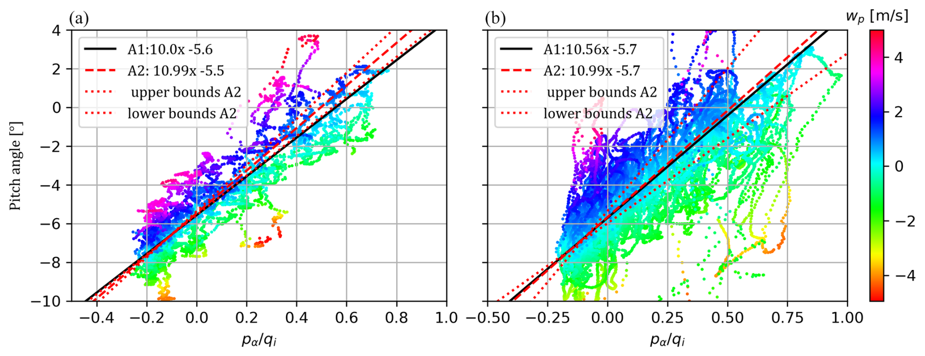
Figure 8 Relationship between the p_α/q_i [–] and the pitch angle [°], for (a) 2017/2018 and (b) 2019/2022, color coded based on the vertical velocity of the aircraft (w_p [m s⁻¹]). The black lines present the relationship, based on a simple linear regression data where |w_p|<1.5 (represented by Eq. A1). The red lines present the correction of the angle of attack based on seven pitching maneuvers and 76 flight legs (represented by Eq. A2; see Table 3).

An alternative approach to look at the correction factors for α is to look at speed runs and plot p_α/q_i and the pitch angle, with respect to the vertical velocity of the aircraft w_p as proposed by Hartmann et al. (2018). Table S1 shows the speed runs that were used for the alternative calibration of α (Eq. A1). Figure 8 shows the relationship between $\frac{p_{\mathit{\alpha }}}{q_i}$ and the pitch angle for all maneuvers in 2017/2018 and 2019 and 2022, including only segments where w_p was smaller than 5 m s⁻¹. Clearly, the alternative calibration based on the speed run data (w_p < 1.5 m s⁻¹; black curve) fits the data quite similarly compared to the first calibration approach (Eq. A2, red curve with uncertainty boundaries; based on pitching oscillations and straight flight legs). The fact that both methods provide quite similar calibration curves shows that both approaches can be used to calibrate α.

3.2 Wind quality evaluation

The quality of the final wind product obtained from the ASK-16 measurement flights can be assessed from a different perspective, using multiple analysis results. First, we assess the quality of the wind vector based on the calibration results from the different maneuvers as presented in Sect. 3.1. In general, the calibration results have shown that the effect of aircraft movement on the measured wind vector can be significantly reduced by the obtained calibration parameters (see Table 3). The obtained parameters seem to be robust as they show little variation during different flight conditions (wind speed, temperature, humidity, measurement altitude, etc.).

Additionally, yaw and pitch maneuvers can provide us with information about the remaining uncertainty of the wind components. Sideslip and angle-of-attack calibration results show that the remaining uncertainty (precision; here defined as standard deviation during pitching/yawing maneuver) of w, u, and v is in most cases between 0.2 and 0.25 m s⁻¹ when the vertical speed of the aircraft is on average 0.21 m s⁻¹. Considering that the horizontal and vertical movement of the aircraft is generally much smaller during real measurement flights, the real accuracy of w, u, and v is expected to be smaller.

Another way to look at the quality of the calibration is to look at the wind vectors obtained during wind square maneuvers. Figure 9 shows uncalibrated and calibrated wind speed, wind direction (Fig. 9a and b), u, and v (Fig. 9d and e) during a wind square maneuver flown on 21 September 2019. Here, the uncalibrated wind vectors show a clear change of u and v with the horizontal movement of the aircraft (yaw angle ψ), indicating that the wind vectors are affected by the movement of the aircraft. This bias is not visible in the calibrated wind vector, where we see a more homogeneous wind field and a generally smaller variability in wind speed, wind direction, u, and v. Considering that the wind calibration parameters have been obtained independently, these results show that the calibration parameters that reduce aircraft-movement-induced effects on the wind vectors can be successfully applied to other flight data.

A third way to assess the quality of the obtained wind vectors is to assess the data in frequency space. Figure 10 shows power spectra of the calculated u, v, and w; the measured temperature; and the abundance of CH₄ CO₂ and H₂O for a flight leg (ca. 26 km long) flown on 21 August 2019 over northeast Germany. Flight legs were flown at an altitude of 150–230 m a.g.l., the wind was coming from the west, and the boundary layer thickness during these flights was between 2250 and 2300 m above the surface (see Sect. S2). In Fig. 10a, we clearly see that the wind follows a $-\mathrm{5}/\mathrm{3}$ drop-off, describing the energy decay of turbulent elements according to Kolmogorov's law (Foken, 2017). Similar observations were made by Metzger et al. (2012), and these results suggest that the different frequencies were appropriately represented in the measurements.

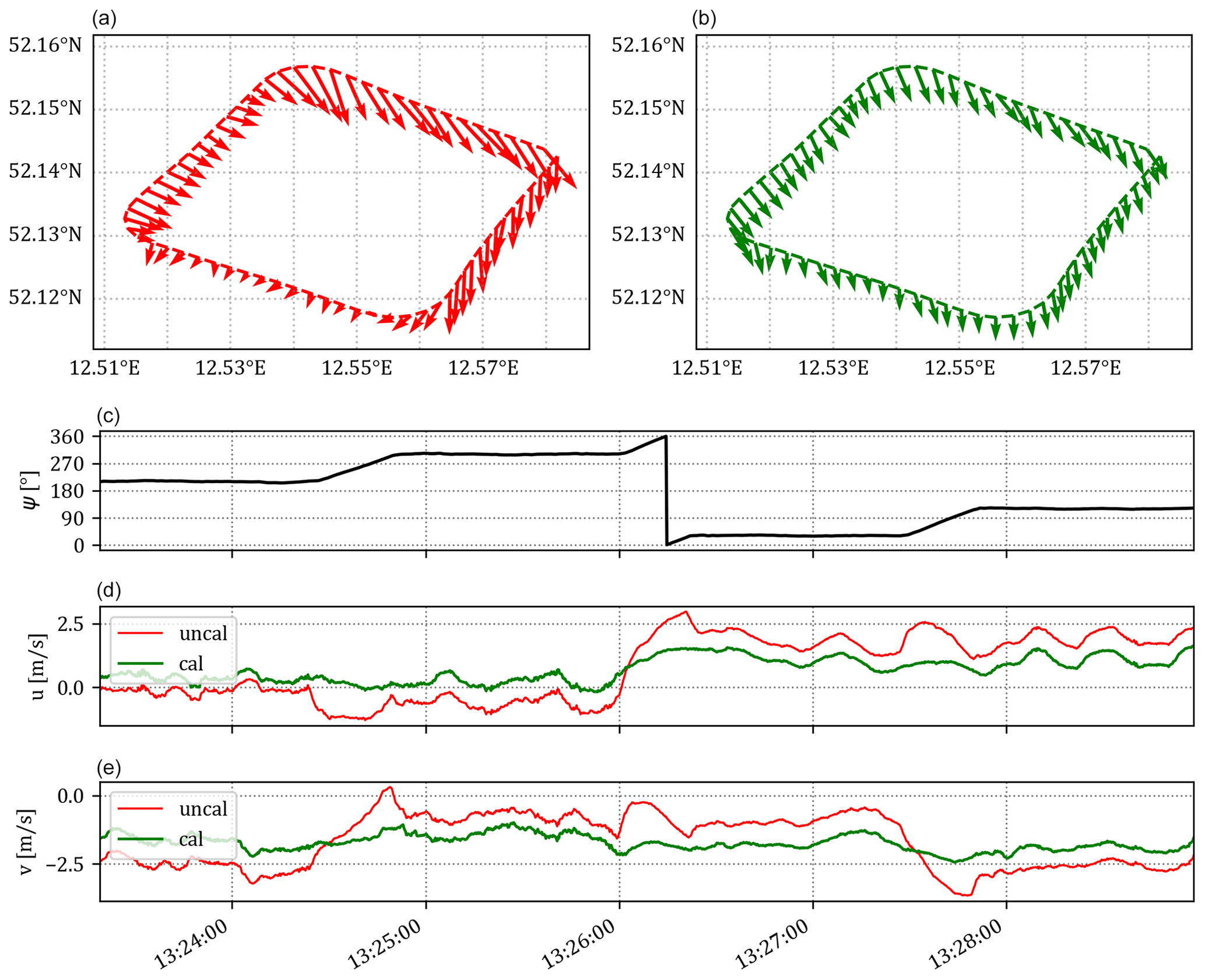
Figure 9 Comparing calibrated (cal; green, b) and uncalibrated (uncal; red, a) wind vectors for a wind square maneuverer (duration: ca. 5.5 min), flown close to Bad Belzig, Germany (52.1427° N, 12.5952° E), on 21 September 2019. The heading as measured by the INS–GNSS (c) is plotted above both horizontal wind components u and v (d, e) to indicate the effect of the aircraft movement on the wind vector before and after calibration.

The spectra of the measured gases and temperature, on the other hand, did not follow the $-\mathrm{5}/\mathrm{3}$ drop-off as nicely. The observed spectral shapes indicate that these datasets contained more white noise. These results are similar to spectral analyses that were earlier reported by Wolfe et al. (2018) and Hartmann et al. (2018), who also identified noise in the power spectra of CH₄ and CO₂ data obtained from closed-path LGR fast gas analyzers. However, as the white noise is generally uncorrelated to the wind data, this should not affect the obtained fluxes (see, e.g., Hartmann et al., 2018). The H₂O power spectrum shows clear signal attenuation (loss in signal) at higher frequencies, which is common for closed-path systems (e.g., Polonik et al., 2019). This will, however, contribute to only small losses of fluxes (covariances) for the aircraft flying approximately 150–230 m above the surface. Cospectra (Sect. S3, Fig. S5) also clearly indicate that the noise signal (visible in the spectral plots) is not correlated with the vertical wind and does not cause any artificial flux signal.

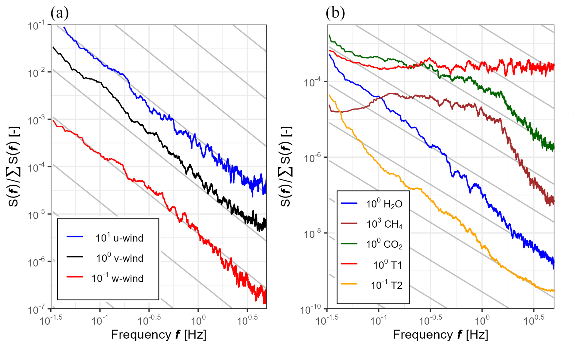
Figure 10 Power spectra of the fluctuations of (a) the 3D wind vector, (b) the measured gases, and the air temperature data (T1: thermocouple; T2: Vaisala Pt100 sensor). The raw spectra are obtained from a 10 min time series and are smoothed (Daniell kernel from stats library in R), normalized by total spectral power, and therefore non-dimensional. All straight slopes show a $-\mathrm{5}/\mathrm{3}$ decrease, showing the theoretical decay of turbulence with increasing frequency according to (gray lines) Kolmogorov's law (Foken, 2017). These power spectra show flight data from one flight leg (flight date: 21 August 2019; altitude: between 220 and 310 m a.s.l.) over a heterogeneous landscape (land use: mainly forest and lakes), close to the Müritz national park in Germany.

3.3 Fluxes and footprints over northeast Germany

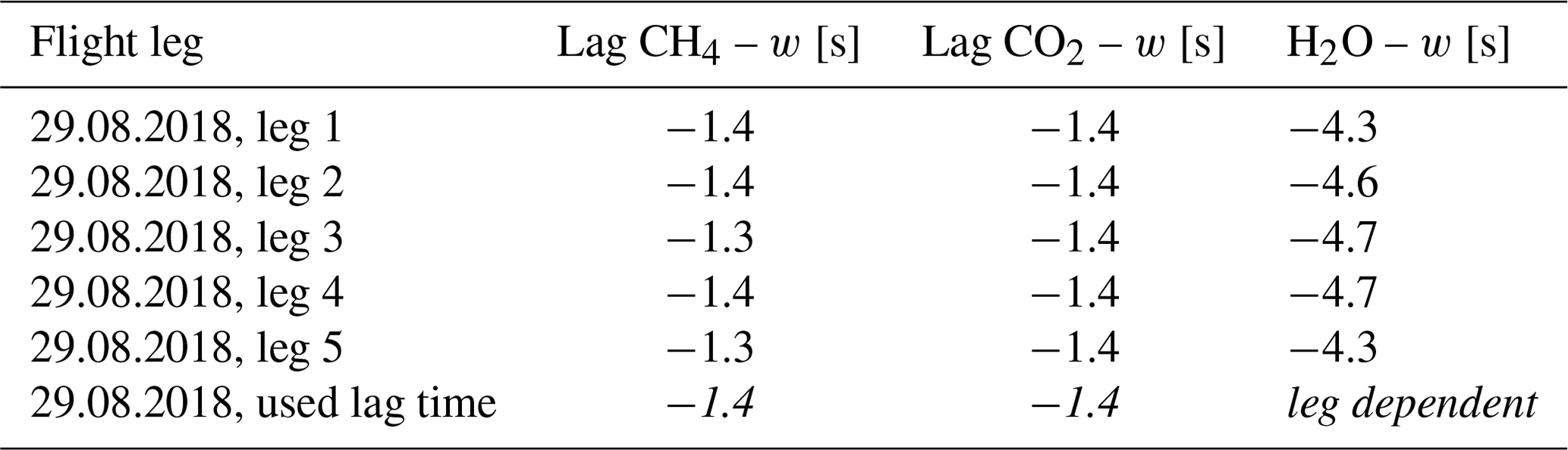
To illustrate the flux output that was obtained with the eddy4R packages, we used flight data from 29 August 2018 flown in the surroundings of Demmin (53.9056° N, 13.0498° E) and the Kummerower See (53.7991° N, 12.8499° E; also known as Lake Kummerow) in northeast Germany. During this measurement flight, five flight legs were flown over a heterogeneous transect with lake, forest, agricultural, grassland, and peatland segments (Fig. 12e). Figure 11 shows exemplary wavelet- and Reynolds-based CO₂ fluxes for the first flight leg (northeast to southwest). Obtained lag times between the gas analyzer (Picarro) and the wind are documented in Table 4.

Table 4 Obtained lags (in seconds) between the measured gases by the Picarro G2311-f and the calculated wind vector for five flight legs on 29 August 2018. Fluxes for these flights and a quality assessment of these fluxes are provided in Figs. 11 and 12 and Table 5. Time lags for latent heat fluxes were flight leg dependent, meaning that the lag time of that specific flight leg was used for time synchronization (italics).

The dominant blue color in the cross-scalogram (Fig. 11a) reveals that we mainly measured an uptake of CO₂ (negative fluxes). The spatial pattern of the fluxes (Fig. 11d) is similar for the wavelet-based and Reynolds-based CO₂ fluxes, although the Reynolds-based fluxes are generally somewhat smaller and more noisy (due to undersampled low frequencies). This is expected, as wavelet-based fluxes contain lower-frequency information that is not present in the 2 km Reynolds-based flux data. In general, the highest CO₂ uptake is observed during the last 6 to 8 km of the flight tracks and is then decreasing until the southwestern end of the track.

The data in Fig. 11 only present the spatially measured CO₂ flux for one flight leg. To get a broader overview of the measured fluxes, Fig. 12 shows information about the fluxes itself (a–c), their footprints (averaged over all legs; see Fig. 12d and e), and the variability in fluxes (a–c) measured during the different flight legs. Clearly, the CO₂ fluxes measured during the other flight legs were also negative, and the average spatial CO₂ flux pattern was similar to the pattern already observed in Fig. 11. CH₄ fluxes, on the other hand, were positive and showed a mirroring trend, with the largest peak in emissions in the region where the largest uptake of CO₂ was observed. These peaks in methane emissions and carbon uptake are connected to areas with high percentages of forest and peatland coverage. CO₂ uptake was largest for an area with 52.6 % of forest and 13.9 % of peatland coverage (63.5 % of total coverage, green triangles in Fig. 12), and CH₄ fluxes were largest for an area with 50 % of forest and 22 % of peatland coverage (72 % of total coverage, red dots in Fig. 12; according to CLC 2018, version 2020, European Environment Agency, 2020). At the same time, the highest variability in latent heat fluxes is observed in the region where the highest percentage of peatland was observed (see Fig. 12c). Figure 12 already provides a quick insight about how measured fluxes can be connected to land surface properties. Past research has already revealed that larger airborne eddy covariance datasets can have a large potential in connecting fluxes and surface properties (e.g., Metzger et al., 2013; Serafimovich et al., 2018; Vaughan et al., 2021; Zulueta et al., 2013).

Figure 11 CO₂ flux data for a flight leg (leg 2; see Table 5) flown over northeast Germany (close to Demmin, Mecklenburg-Vorpommern, Germany), which was recorded on 29 August 2018. The cross-scalogram (a) shows positive (red, upward fluxes) and negative covariances (blue, downward fluxes) between CO${}_{\mathrm{2}}^{\prime }$ (b) and w^′ (c). In this case, blue color dominates in the cross-scalogram, indicating that uptake of CO₂ dominates during this flight leg at this time of the year. The final scale-integrated fluxes at high resolution (light-blue area) and the 2 km integrated fluxes (dark-blue line) are shown on the bottom in comparison to Reynolds decomposed fluxes (dotted black lines, calculated every 200 m for 2 km windows). Flight distance as presented on the x axis of panel (a) is representative for all panels. The latitude on the x axes (UTM, zone 33N) corresponds with coordinates in Fig. 12.

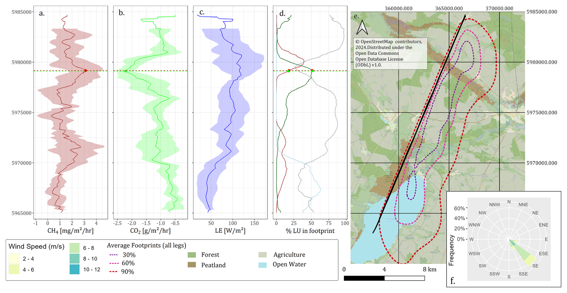
Figure 12 Transect with measured CO₂, CH₄, and LE (latent heat) fluxes over a heterogeneous landscape in northeast Germany (close to Demmin; date: 29 August 2018). The location of the transect is shown in panel (e) (background: OpenStreetMap). Flux data in panels (a)–(c) are based on airborne flight data from five flight legs, where thicker lines show the median fluxes and the colored areas surrounding these lines indicate the standard deviation of these fluxes. Besides the measured fluxes, land use cover and average footprints (based on footprints from all five individual legs) are shown in panels (d) and (e). The land use classification presented in this map (e) is a simplified version of the Corine land cover classification of 2018 (Corine Land Cover (CLC) 2018, version 2020_20u1 (European Environment Agency, 2020)). Panel (f) shows a wind rose with the dominant wind direction(s) during the five flight legs.

3.4 Flux quality evaluation

After assessing the quality of the wind vector, the quality of the measured fluxes also needs to be evaluated. Table 5 shows the results of the stationarity assessment, the assessment of the integral turbulence characteristics, and the calculated detection limits of the fluxes for the measurement flight. As a reference, the Reynolds fluxes for all the flight legs are also provided. Mind that these fluxes do not represent the variability in the fluxes (as shown in Fig. 12) but rather the overall leg-averaged flux.

Table 5 Quality assessment of five flight legs flown on 29 August 2018, close to Demmin, Germany (see Fig. 12). The table includes information about the leg-based fluxes (Reynolds Fluxes), the integral turbulence characteristics (ITCS), stationarity, and the detection limits of the measured fluxes according to Billesbach (2011).

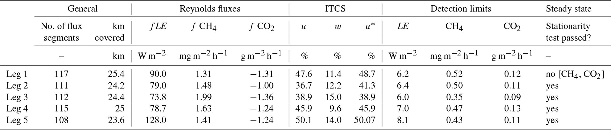
The detection limits of the fluxes are generally much lower than the measured leg-based fluxes. Most of the 200 m based fluxes are also above these detection limits, indicating that the observed fluxes in this region are high enough to be measured with our current setup. As airborne eddy covariance fluxes can only be measured under stationary conditions, stationarity needs to be assessed. In most cases, the stationarity test was also passed, except for the first flight leg, where the stationarity requirements were not met for CH₄ and CO₂ fluxes. The integral turbulence characteristics are ≤ 100 % for all flight segments during all legs, indicating that the turbulence conditions were adequate during the flight.

One way to look at the uncertainty of the calculated fluxes is to evaluate the variability in obtained fluxes for repeated flight paths. Figure 12 clearly shows the variability and therewith the uncertainty of the fluxes during a flight over a heterogeneous landscape indicated by the shading. The uncertainty is calculated as the standard deviation of five repeated measurements (flight legs) per 200 m segment. Although part of the differences in fluxes might be assigned to differences in footprints, it does give an indication of the uncertainty of the obtained fluxes. Based on the repeated flight legs, the variability in CH₄ fluxes was 86.2 ± 57.7 %, the variability y in CO₂ fluxes was 32.9 ± 12.9 %, and the variability in latent heat fluxes was 36.6 ± 13.0 % per 200 m segment. Clearly, Fig. 12 shows that even when we consider these uncertainties, general trends in energy and matter fluxes can still be clearly identified.

Another way to evaluate the uncertainty of the calculated fluxes is to calculate the systematic (SE) and random statistical errors (RE) according to Mann and Lenschow (1994) and Lenschow and Stankov (1986). Table 6 summarizes these errors both for Reynolds-based and wavelet-based fluxes. Please mind that these errors mainly describe the errors of single segments (except for the relative error according to Billesbach, 2011). Larger random errors were generally observed for smaller CH₄ fluxes, which is in agreement with the observations by Wolfe et al. (2018). As we calculate a flux over a 2 km window for every 200 m, flux segments overlap spatially, which will decrease the error over a specific region. Generally, the systematic errors are very small (in most cases up to 1 %), and the random errors for single leg segments are much larger (< 100 % for Reynolds fluxes and > 100 % for wavelet fluxes). As the random shuffling method by Billesbach (2011) can also be used to determine the random error of the flux (e.g., Dong et al., 2021), this random flux error that is representative for a leg-averaged flux was also added to the table.

Table 6 Error assessment of airborne fluxes for the ASK-16 platform. This table provides an overview of the systematic errors (SE) and the random errors (RE) of the calculated CO₂, CH₄, and LE fluxes (both wavelet and Reynolds) in percentage (%). Errors were calculated according to Mann and Lenschow (1994), Lenschow and Stankov (1986), and Billesbach (2011). All flux errors are given for flight segments (a flux is calculated for a 2 km window every 200 m). The random flux error according to Billesbach (2011) was only calculated for the entire flight leg. Numbers in italics provide summary statistics (total number of segments, average SE and RE) for the whole measurement flight.

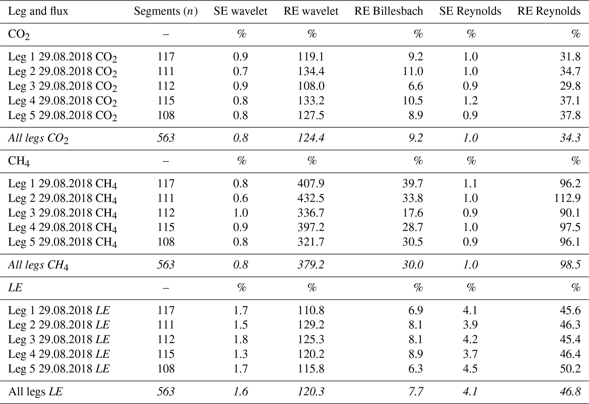
The obtained magnitudes of the systematic and random errors are similar to earlier studies (e.g., Wolfe et al., 2018; Metzger et al., 2012). The difference in errors between Reynolds- and wavelet-based fluxes can be explained by the fact that Mann and Lenschow (1994) assume that fluxes over a 2 km window only use flux data within that window. This is not the case for wavelet-based fluxes, where time series information from the entire lag is used for the derived covariances within a given window. This was already described in Wolfe et al. (2018) and could explain the much larger random errors for the wavelet-based fluxes. The errors based on the repeated flight legs (Fig. 12) and the Reynolds-based fluxes are much more similar and are expected to be more realistic. Overall, this suggests that random errors of individual leg segments (here 2 km averaged fluxes) are rather in the range of 30 %–40 % for LE and CO₂ and 80 %–100 % for CH₄.

4 Conclusion and outlook

In this paper, we have described the ASK-16 airborne measurement platform, which can be used to measure airborne eddy covariance fluxes. Here, we have demonstrated that this platform can produce a 3D wind vector that has a similar quality to other airborne eddy covariance measurement platforms (Metzger et al., 2011; Mallaun et al., 2015; Hartmann et al., 2018). Although the spectra of the gas measurements and the fast temperature showed white noise, this should not affect fluxes as noise is uncorrelated to the measured wind (Hartmann et al., 2018). This paper has also provided a way to evaluate the quality of the obtained fluxes with the help of different tools that are available within the eddy4R toolbox, including stationarity tests, ITCS, and the identification of detection limits. Detection limits for the turbulent fluxes were between 6–8 W m⁻² for LE, 0.35–0.52 mg m⁻² h⁻¹ for CH₄, and 0.09–0.13 g m⁻² h⁻¹ for CO₂.

The flux products that can be obtained for the ASK-16 platform were illustrated using exemplary flux transects over northeast Germany. The measurement errors of the fluxes have similar magnitudes to previously well-established airborne platforms (e.g., Metzger et al., 2012; Wolfe et al., 2018). Additionally, the flux transect data have illustrated that the ASK-16 can be used to measure turbulent fluxes over a heterogeneous landscape, such as northeast Germany, and that the obtained fluxes can be linked to surface properties. Considering the spatial distribution of eddy covariance towers and the potential of airborne platforms to cover large regions, platforms such as the ASK-16 are useful tools to bridge these scales.