Estimating vertical profiles of ice water content and snowfall rate from radar measurements in the G-band

We present theory and simulations to show that at frequencies of order 200 GHz (G-band) the radar cross section (σ_r) of ice particles larger than ∼ a quarter wavelength (0.375 mm) is nearly directly proportional to their mass (m). Hence measurements of radar reflectivity (Z) at this frequency are directly proportional to the ice water content (IWC), with no other assumptions about the shape or breadth of the particle size distribution required. For the same reason, vertically pointing Doppler velocities at this frequency provide the mass-weighted mean vertical velocity of the particles, and the product of Z with the mean Doppler velocity (MDV) is proportional to the snowfall rate (S). This presents the opportunity for straightforward and accurate retrievals of ice microphysics.

We explore the sensitivity of such retrievals to the scattering model for ice particles. We find that all seven models examined, four with random orientation and three with horizontal orientation, have σ_r∝m in this regime, but that the coefficient of proportionality varies between models. The dominant factor controlling this coefficient is the mass-size relationship for the ice particles, and specifically the mass of a wavelength-sized ice particle. If this information is known, or can be assumed, then the ice population parameters above can be retrieved with high accuracy. For mass-weighted mean diameters D_m>0.5 mm the variation in the IWC–Z relationship is within ≈ 30 %, and the variation in the S–(Z×MDV) relationship is within ≈ 15 %.

The method is applied to retrieve IWC and S during two case studies, with measurements from the GRaCE 200 GHz Doppler radar at Chilbolton Observatory in the UK. In the first of these case studies, retrieved snowfall rates from particles falling aloft in a precipitating ice cloud were compared to gauge data at the surface. In the second case study, retrieved ice water contents from a deep non-precipitating stratiform ice cloud were compared to measurements made using an evaporative water content probe on board the Facility for Airborne Atmospheric Measurements (FAAM) BAe-146 instrumented research aircraft. In both cases a statistical comparison was necessary because of imperfect colocation of the radar measurements and in-situ/gauge sampling. The measurements fall within the distributions of the retrieved water content and snowfall fields, and follow consistent trends with time (Case 1) and height (Case 2), providing evidence that this method produces realistic retrievals.

Application of the same technique at even higher radar frequencies would allow clouds with smaller particles (e.g. in high altitude cirrus clouds) to be characterised. Because of the increased gaseous attenuation at such frequencies, the latter may be more practical from airborne or spaceborne platforms.

1 Introduction

Recent technological advancements have enabled the development of G-band (110–300 GHz) radars with high enough sensitivities for atmospheric remote sensing. There have been a number of successful ground-based and airborne demonstrators such as VIPR in USA (Cooper et al., 2018, 2021; Millán et al., 2024; Roy et al., 2020, 2022; Lamer et al., 2021), GRaCE in UK (Courtier et al., 2022, 2024, 2025), CloudCube in USA (Socuellamos et al., 2024a, b, c), and more recently GRaWAC in Germany (Bühler et al., 2025). As hypothesised by Battaglia et al. (2014), the demonstrator instruments have shown that measurements in the G-band contain valuable information for a variety of atmospheric scenarios. In terms of humidity and liquid clouds, G-band data has been used successfully to profile water vapour (Roy et al., 2020) and, when combined with other frequencies, to retrieve small amounts of liquid water in warm shallow clouds (Socuellamos et al., 2024c) and improve microphysical retrievals in light rain (Courtier et al., 2024). In the ice phase, Lamer et al. (2021) and McCusker et al. (2025) highlight that using a dual-frequency pair inclusive of G-band data allows sizing of smaller ice particles than has been possible using lower frequencies such as Ka and W bands.

Although there is currently no G-band cloud radar in space, with the highest frequency space-borne radars operating in the W-band (on-board CloudSat (Marchand et al., 2008) and the Doppler radar on EarthCARE (Illingworth et al., 2015)), the aforementioned findings suggest that a spaceborne G-band radar could be on the horizon. Indeed, GRaCE and CloudCube are intended as demonstrators for future satellite missions. Ideally such missions will exploit the benefits of multi-frequency observations; however it is also important to explore simpler methods, which may be accessible using a single frequency, or provide a robust first estimate of the microphysical state of the cloud before refinement using dual-frequency ratios (which typically have higher uncertainty). The success of EarthCARE's Doppler capability (Kim et al., 2025) also motivates us to consider the information content of Doppler measurements, in addition to reflectivity.

Algorithms that currently exist to retrieve ice water content (IWC) and snowfall rate (S) from radar measurements can be of varying complexity, but the simplest methods are direct statistical relationships between reflectivity and ice population properties, i.e. Z–IWC or Z–S relationships. These relationships may be used directly to retrieve particle properties, or may form the initial estimate for an optimal estimation retrieval (this is the case, for example, in the EarthCARE cloud and precipitation microphysics (C-CLD) algorithm (Mroz et al., 2023), where the estimate is subsequently refined using the Doppler velocity information).

However, it is well documented that the relationship between Z and microphysical parameters of interest is not unique, and varies considerably (e.g. Protat et al., 2016; Matrosov and Heymsfield, 2008). Brown et al. (1995) show IWC as a function of Z at W-band, computed from a large number of in-situ particle size distributions. The IWC for a given reflectivity is spread over approximately an order of magnitude across the various cloud samples, with typical uncertainties on the order of a factor of two, and this variation is driven by variations in the breadth and shape of the particle size distribution (PSD), i.e., how wide or narrow the range of particle sizes is, and how the particle sizes are distributed around the mean. Retrieving S from reflectivity presents similar problems, with order of magnitude variability in the value of S for a given Z (Hiley et al., 2011; Fuller et al., 2023 and references therein). Because Z and IWC (or Z and S) are proportional to different moments of the PSD, their interrelationship is sensitive to what that PSD shape and width is. Interestingly, the variability in the IWC–Z relationship decreases as Z increases, due to increased non-Rayleigh scattering (Brown et al., 1995) and it is this phenomenon that we will exploit in the current study.

In this manuscript, we explore the usefulness of radar reflectivity and Doppler velocity in the G-band for estimating IWC and S, with a view towards a future spaceborne G-band radar. We consider theory and simulations, along with measurements from a ground-based G-band radar, to determine what information is required for accurate retrievals. We show that IWC and S can be retrieved with a single frequency G-band radar provided that the mass of a wavelength-sized particle is known or can be assumed, while the details of the PSD breadth and shape are not required. Two case studies are provided to illustrate the practical application of the theory, and to demonstrate that the retrievals are consistent with in-situ measurements of IWC and S. This work presents the first known retrievals of ice cloud and snowfall properties using a G-band radar, representing a major step forward in the use of high-frequency radar for atmospheric remote sensing. Unlike traditional optimal estimation approaches, which are computationally intensive but widely adopted, the method introduced here is both computationally efficient and robust, offering a practical alternative without compromising reliability.

2 Parameters of interest

Our first measurement parameter is the equivalent radar reflectivity factor Z:

$$\begin{array}{}\text{(1)}& Z={\mathrm{10}}^{\mathrm{18}}{\displaystyle \frac{{\mathit{\lambda }}^{\mathrm{4}}}{{\mathit{\pi }}^{\mathrm{5}}|K_{\mathrm{water}}{|}^{\mathrm{2}}}}\underset{\mathrm{0}}{\overset{\mathrm{\infty }}{\int }}N\left(D\right){\mathit{\sigma }}_{\mathrm{r}}\left(D\right)\mathrm{d}D,\end{array}$$

and we denote the logarithmic equivalent as dBZ = 10log ₁₀(Z). N(D) is the particle size distribution (PSD, m⁻⁴), such that there are N(D)dD ice particles with maximum dimension in the interval $[D,D+\mathrm{d}D]$, and σ_r(D) is the radar cross section (m²) of each ice particle of that size. λ is the free space wavelength, 1.5 mm at 200 GHz. The factor 10¹⁸ is present to convert the SI units of N, σ_r and λ to the conventional reflectivity unit of mm⁶ m⁻³. We choose to normalise Z using $|K_{\mathrm{water}}{|}^{\mathrm{2}}=\mathrm{0.93}$, which is the value for liquid water at cm-wavelengths, following the approach of Hogan et al. (2006).

In addition to Z, we can also consider the mean Doppler velocity (MDV), which is the average of the vertical velocity of the particles v(D) (equal to the still-air fall speeds of the particles, plus any vertical air motion), weighted by their radar cross sections and PSDs, i.e.

$$\begin{array}{}\text{(2)}& \mathrm{MDV}={\displaystyle \frac{{\int }_{\mathrm{0}}^{\mathrm{\infty }}N\left(D\right){\mathit{\sigma }}_{\mathrm{r}}\left(D\right)v\left(D\right)\mathrm{d}D}{{\int }_{\mathrm{0}}^{\mathrm{\infty }}N\left(D\right){\mathit{\sigma }}_{\mathrm{r}}\left(D\right)\mathrm{d}D}}.\end{array}$$

Our retrieval parameters are IWC and S, which can be written in terms of the PSD as:

$$\begin{array}{}\text{(3)}& {\displaystyle }\mathrm{IWC}=\underset{\mathrm{0}}{\overset{\mathrm{\infty }}{\int }}N\left(D\right)m\left(D\right)\mathrm{d}D\text{(4)}& {\displaystyle }S=\underset{\mathrm{0}}{\overset{\mathrm{\infty }}{\int }}N\left(D\right)m\left(D\right)v\left(D\right)\mathrm{d}D,\end{array}$$

where m is the particle mass (in kg).

Note that the equations above give IWC with units of kg m⁻³ and S with units of kg m⁻³ m s⁻¹. Thus to express IWC in g m⁻³ and S in mm h⁻¹ (as we do in the following section) requires multiplication by 10³ and 3600 respectively.

As we will see shortly, at high frequencies such as G-band, Z becomes almost directly proportional to IWC, while the product (Z×MDV) becomes nearly directly proportional to S. This is in stark contrast to the behaviour at lower frequencies, such as Ka-band, and is a result of the non-Rayleigh scattering which occurs when the particle becomes comparable in scale to the wavelength.

3 Simulations of ice and snow parameters using realistic particle scattering models

In this section, we perform simulations of IWC and S using Eqs. (3) and (4). To illustrate the concept, we use the Large Plate Aggregate mixture from the ARTS scattering database (Eriksson et al., 2018), which combines pristine plate habits to cover the smaller sizes of the PSD with aggregates of plates to represent the larger sizes. The particles are randomly oriented in 3D, and details on their mass can be found in Sect. 5 and Table 1. We assume an exponential PSD: $N\left(D\right)=N_{\mathrm{0}}\exp (-\mathrm{\Lambda }D)$ where the slope parameter Λ controls the breadth of the distribution (and hence the average particle size), while the intercept parameter N₀ scales the particle concentrations up and down to allow IWC to vary independently of particle size.

Table 1 Relevant coefficients for the four particle mixtures from the ARTS scattering database (Eriksson et al., 2018) and the three habits from the rimed database of Mroz and Leinonen (2023) used in this study.

^∗ Since the shape data is not available for the particles from the database of Mroz and Leinonen (2023), the values of $c_{R_{\mathrm{g}}}$ cannot be calculated directly. Thus we use the value of $c_{R_{\mathrm{g}}}\approx \mathrm{0.287}$ suggested by Leinonen and Szyrmer (2015).

3.1 Ice Water content

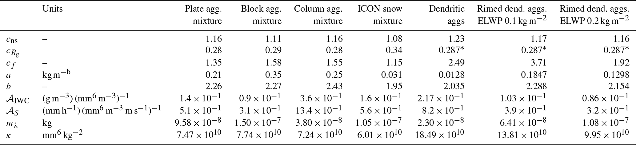
Simulations of IWC are presented in Fig. 1. The left column shows IWC versus radar reflectivity at C-, Ka-, W-, and G-band.

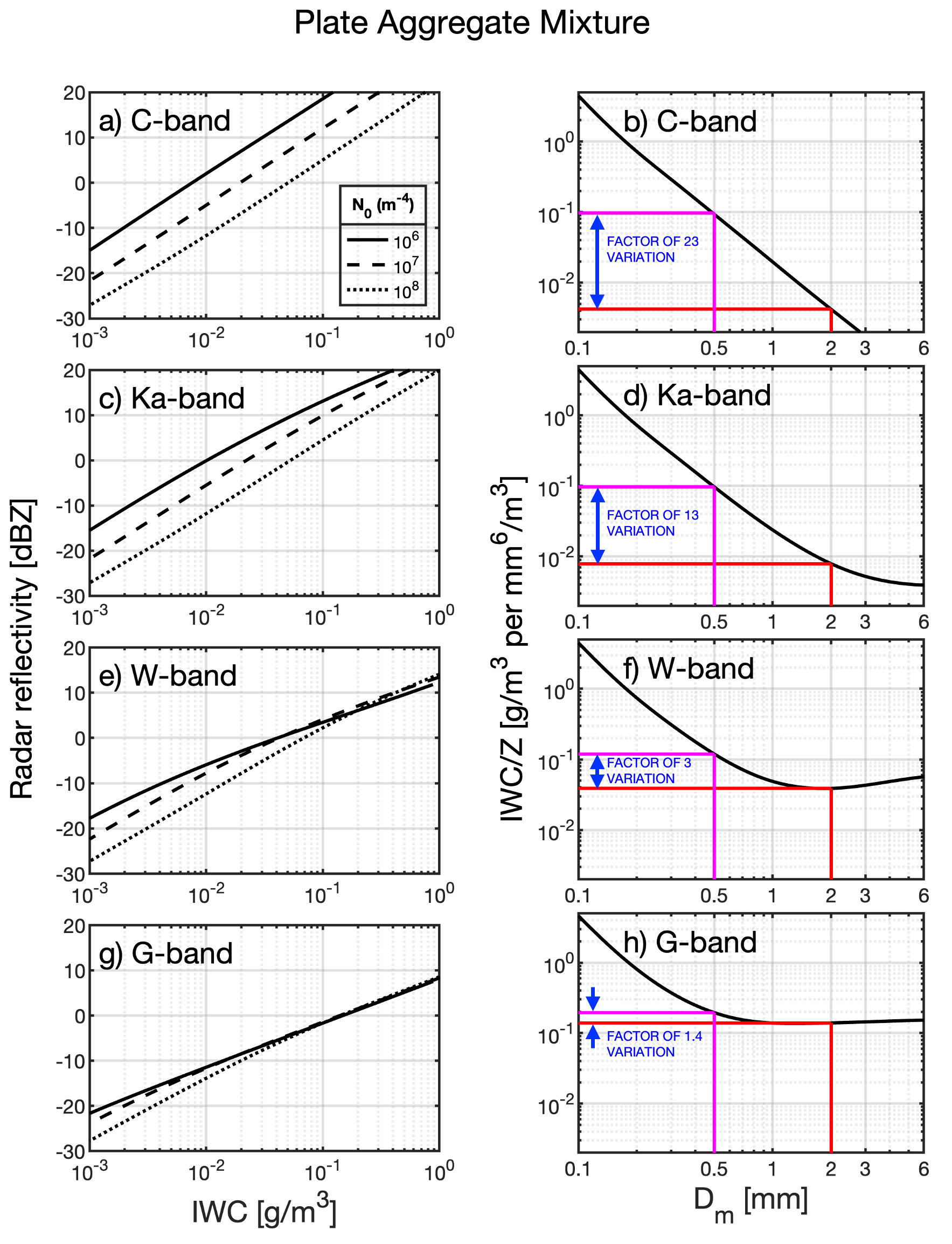
Figure 1 Simulations using the Large Plate Aggregate mixture from the ARTS database, assuming exponential PSDs. The different rows from top to bottom show simulations in the C-, Ka-, W-, and G-band. The left column shows the radar reflectivity (dBZ) for a range of IWC, where the different linestyles represent different values of N₀ in the PSDs. The right column shows the ratio $\mathrm{IWC}/Z$ for a range of D_m.

The three different linestyles show results using N₀=10⁶, 10⁷, 10⁸ m⁻⁴. It is clear from Fig. 1a and c that at lower frequencies in the C- and Ka-bands, the relationship between IWC and Z varies considerably with N₀, while the sensitivity to PSD parameters decreases systematically with frequency (Fig. 1e and g). For example, consider a reflectivity measurement of 0 dBZ. The IWC corresponding to this value is highly sensitive to N₀ in the C- and Ka-bands, with differences of 152 % (C-band) and 137 % (Ka-band) between N₀=10⁶ and N₀=10⁸ m⁻⁴. The difference in IWC between N₀=10⁶ and N₀=10⁸ m⁻⁴ decreases with frequency. There is a smaller (but still considerable) difference of 52 % in the W-band, while the difference in the G-band is much smaller, at 7 %.

The right column shows the ratio $\mathrm{IWC}/Z$ for different values of the mass-weighted mean particle diameter

$$\begin{array}{}\text{(5)}& D_{\mathrm{m}}={\displaystyle \frac{{\int }_{\mathrm{0}}^{\mathrm{\infty }}N\left(D\right)m\left(D\right)D\mathrm{d}D}{{\int }_{\mathrm{0}}^{\mathrm{\infty }}N\left(D\right)m\left(D\right)\mathrm{d}D}}.\end{array}$$

At C- and Ka-band, the ratio $\mathrm{IWC}/Z$ decreases continuously with D_m (Fig. 1b and d). This means there would be large uncertainties associated with retrieval algorithms based on a direct relation between Z and IWC, because D_m is unknown a-priori. At higher frequencies, the variation in $\mathrm{IWC}/Z$ becomes smaller, particularly at larger D_m. Figure 1d shows that in the W-band $\mathrm{IWC}/Z$ steadily decreases at small D_m, reaching a minimum at around 2 mm before slightly increasing again at large D_m. At G-band (Fig. 1f), the ratio approaches an almost constant value for sufficiently large D_m.

The variation in $\mathrm{IWC}/Z$ with D_m in the interval 0.5–2 mm is a factor of 23 at C-band, 13 at Ka-band, 3 at W-band, but only a factor of 1.4 at G-band (corresponding to a 33 % variation relative to the mean). In other words, a direct retrieval of IWC from Z in the G-band would have considerably lower uncertainties than at lower frequencies.

In this illustration we have used a single scattering model. The sensitivity to this choice is explored further in Sect. 5.

3.2 Snowfall Rate

Figure 2 shows simulations related to the snowfall rate S. The left column shows the product Z×MDV for a range of S values. As above, the different linestyles show results using different values of N₀. The results mirror those for IWC shown in Fig. 1, with the sensitivity of the simulations to N₀ decreasing with frequency. For a measurement of $Z\times \mathrm{MDV}=\mathrm{1}$ mm⁶ m⁻³ m s⁻¹, the difference in S between N₀=10⁶ and N₀=10⁸ m⁻⁴ is 137 %, 122 %, 24 %, and 13 % for C-, Ka-, W-, and G-band, respectively.

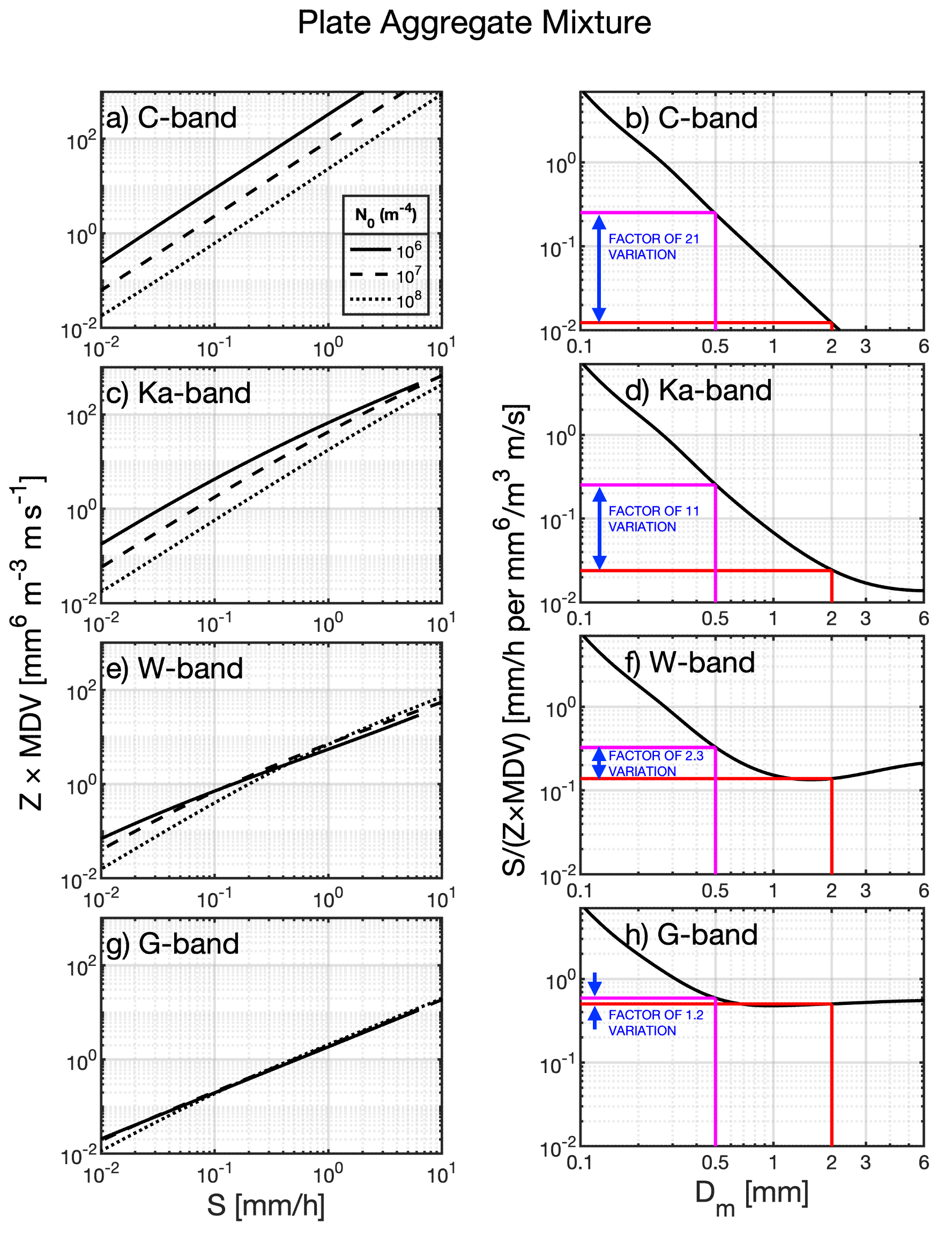
Figure 2 As in Fig. 1, but here the left column shows Z×MDV for a range of S, and the right column shows the ratio $S/(Z\times \mathrm{MDV})$ for a range of D_m.

The right column shows the ratio $S/(Z\times \mathrm{MDV})$ for a range of D_m. These simulations also mirror those presented for $\mathrm{IWC}/Z$, whereby the ratio decreases with D_m in the C- and Ka-bands, but becomes more constant at large D_m in the G-band. The $S/(Z\times \mathrm{MDV})$ ratio varies by a factor of 1.2 for D_m between 0.5 and 2 mm in the G-band (corresponding to a 15 % variation relative to the mean), while for C-, Ka-, and W- bands the ratio varies by factors of 21, 11 and 2.3 respectively, which again suggests that S can be retrieved from measurements of Z and MDV in the G-band.

4 Theory

In the previous section, G-band scattering simulations showed that the ratios $\mathrm{IWC}/Z$ and $S/(Z\times \mathrm{MDV})$ approach a near constant value for values of D_m greater than ≈ 0.5 mm. In this section, we will consider the theory behind those results.

In the Rayleigh regime (i.e. where D≪λ), the radar cross section scales in proportion to the square of the volume of ice within the particle (Doviak and Zrnić, 1993):

$$\begin{array}{}\text{(6)}& {\mathit{\sigma }}_{\mathrm{r}}=\mathrm{36}{\mathit{\pi }}^{\mathrm{3}}{\mathit{\lambda }}^{-\mathrm{4}}{\displaystyle \frac{m^{\mathrm{2}}}{{\mathit{\rho }}_{\mathrm{ice}}^{\mathrm{2}}}}{\left|{\displaystyle \frac{\mathit{ϵ}-\mathrm{1}}{\mathit{ϵ}+\mathrm{2}}}\right|}^{\mathrm{2}}{c}_{\mathrm{ns}},\end{array}$$

where m is the particle mass, ρ_ice is the density of solid ice, and ϵ is the complex dielectric constant of solid ice. As a result, in that regime, we have:

$$\begin{array}{}\text{(7)}& Z_{\mathrm{Rayleigh}}=C_{\mathrm{Rayleigh}}\underset{\mathrm{0}}{\overset{\mathrm{\infty }}{\int }}N\left(D\right)c_{\mathrm{ns}}m(D{)}^{\mathrm{2}}\mathrm{d}D,\end{array}$$

where

$$\begin{array}{}\text{(8)}& C_{\mathrm{Rayleigh}}={\mathrm{10}}^{\mathrm{18}}{\displaystyle \frac{\mathrm{36}|K_{\mathrm{ice}}{|}^{\mathrm{2}}}{\mathrm{0.93}{\mathit{\pi }}^{\mathrm{2}}{\mathit{\rho }}_{\mathrm{ice}}^{\mathrm{2}}}}\end{array}$$

and $|K_{\mathrm{ice}}{|}^{\mathrm{2}}$ is the dielectric factor for ice, which is ≈0.174 at cm and mm wavelengths (Hogan et al., 2006; Westbrook et al., 2007; Hogan et al., 2017). The dimensionless coefficient c_ns is a function of the shape of the particle, and its orientation relative to the polarisation of the radar, and is of order unity. For spherical particles c_ns=1. The Rayleigh Gans Approximation (RGA, see McCusker et al., 2019 and references therein) also assumes that c_ns≈1, reflecting its assumption that the scatterer is composed of a weak dielectric, and hence that the electric field incident on any part of an ice particle is equal to the applied field from the radar. In reality, the coupling between neighbouring parts of the ice particle enhances the mean electric field (McCusker et al., 2019), and increases c_ns to values larger than one. For example, Hogan et al. (2017) suggest that for aggregates of non-spherical ice crystals, $\mathrm{1}<c_{\mathrm{ns}}<\mathrm{2}$. In what follows, we will assume that c_ns is independent of D and can be taken outside the integral in Eq. (7).

Evidently Z_Rayleigh does not scale in proportion to IWC. To convert from one to the other, it is therefore necessary to independently estimate the shape and width of the PSD (and to know the relationship between m and D).

There is extensive literature (e.g. Locatelli and Hobbs, 1974; Mitchell et al., 1990) that suggests ice particle mass and maximum dimension are connected to one another statistically, via a power law relationship, i.e. m=aD^b. Such power law relationships for aggregates and complex crystals are indicative of a geometry that is statistically fractal, with fractal dimension equal to b. For aggregates, the exponent b is typically ≈2, and this leads to $Z_{\mathrm{Rayleigh}}\propto {\int }_{\mathrm{0}}^{\mathrm{\infty }}{D}^{\mathrm{4}}N\left(D\right)\mathrm{d}D$, while $\mathrm{IWC}\propto {\int }_{\mathrm{0}}^{\mathrm{\infty }}{D}^{\mathrm{2}}N\left(D\right)\mathrm{d}D$. Again, this emphasises that at low frequencies (where scattering is close to the Rayleigh regime), Z is a significantly higher moment of the PSD than the ice water content or snowfall rate.

Equation (7) is appropriate for scattering by ice particles at centimetre wavelengths; however at millimetre wavelengths non-Rayleigh effects become increasingly important. In this case, the radar cross section has a more complex dependence on particle size. Physically, as the dimensions of the particle become comparable to the wavelength, interference begins to occur between the waves that are scattered from different parts of the particle. We express this non-Rayleigh behaviour via a dimensionless factor f which depends on the size of the particle relative to the wavelength:

$$\begin{array}{}\text{(9)}& Z=C_{\mathrm{Rayleigh}}{c}_{\mathrm{ns}}\underset{\mathrm{0}}{\overset{\mathrm{\infty }}{\int }}N\left(D\right)m\left(D{)}^{\mathrm{2}}f\right(D/\mathit{\lambda })\mathrm{d}D.\end{array}$$

For fractal aggregates, Sorensen (2001) used RGA to deduce the scaling of f when the particle is large enough compared to the wavelength, and found that it had a power law dependence, which for backscattering is:

$$\begin{array}{}\text{(10)}& f\approx c_f{\left({\displaystyle \frac{\mathrm{4}\mathit{\pi }{R}_{\mathrm{g}}}{\mathit{\lambda }}}\right)}^{-b}.\end{array}$$

Here R_g is the radius of gyration, which as we will show later is proportional to D, and the non-dimensional coefficient c_f is of order unity. Berg (2008) used the discrete dipole approximation (DDA) to confirm that this power law scaling is still evident even when RGA is not strictly applicable (such as is the case for ice: e.g. McCusker et al., 2021). Inserting this into Eq. (9), we obtain:

$$\begin{array}{}\text{(11)}& Z\approx C_{\mathrm{Rayleigh}}{c}_{\mathrm{ns}}{c}_f{\left(\mathrm{4}\mathit{\pi }{c}_{R_{\mathrm{g}}}\right)}^{-b}{\mathit{\lambda }}^b\underset{\mathrm{0}}{\overset{\mathrm{\infty }}{\int }}N\left(D\right)m(D{)}^{\mathrm{2}}{D}^{-b}\mathrm{d}D,\end{array}$$

where $c_{R_{\mathrm{g}}}=(R_{\mathrm{g}}/D)$, which as we will demonstrate later has a typical value of around 0.3. Equation (11) is valid provided that the particles dominating the reflectivity are sufficiently large relative to the wavelength. Based on our simulations in Figs. 1 and 2, this occurs when D_m≳0.5 mm. Inserting the mass-size relationship m=aD^b into Eqs. (11) and (3), we obtain our key result, valid in the regime where the particles dominating the radar measurements are comparable to, or larger than the wavelength:

$$\begin{array}{}\text{(12)}& Z\approx \mathit{\kappa }{m}_{\mathit{\lambda }}\underset{\mathrm{0}}{\overset{\mathrm{\infty }}{\int }}N\left(D\right)a{D}^b\mathrm{d}D=\mathit{\kappa }{m}_{\mathit{\lambda }}\mathrm{IWC},\end{array}$$

where the coefficient $\mathit{\kappa }=C_{\mathrm{Rayleigh}}{c}_{\mathrm{ns}}{c}_f(\mathrm{4}\mathit{\pi }{c}_{R_{\mathrm{g}}}{)}^{-b}$ and m_λ=aλ^b is the mass of a wavelength-sized particle i.e. m(D=λ).

In the same way, we can show that

$$\begin{array}{}\text{(13)}& \begin{array}{rl}(Z\times \mathrm{MDV})\approx & C_{\mathrm{Rayleigh}}{c}_{\mathrm{ns}}{c}_f(\mathrm{4}\mathit{\pi }{c}_{R_{\mathrm{g}}}{)}^{-b}{\mathit{\lambda }}^b\\ & \underset{\mathrm{0}}{\overset{\mathrm{\infty }}{\int }}N\left(D\right)m\left(D{)}^{\mathrm{2}}{D}^{-b}v\right(D)\mathrm{d}D=\mathit{\kappa }{m}_{\mathit{\lambda }}S.\end{array}\end{array}$$

It also follows that the mean Doppler velocity is equal to the mass-weighted vertical velocity of the snowflakes.

The results in Eqs. (12) and (13) explain the near-constant values of $\mathrm{IWC}/Z$ and $S/(Z\times \mathrm{MDV})$ for large D_m at G-band in Figs. 1f and 2f. The key parameters in these relationships are therefore m_λ and κ, and we now investigate these factors in depth.

5 Estimation of m_λ, κ, and its components

From Eqs. (12) and (13), we expect $\mathrm{IWC}/Z$ and $S/(Z\times \mathrm{MDV})$ to approach a constant value $\mathcal{A}=\mathrm{1}/\left(\mathit{\kappa }{m}_{\mathit{\lambda }}\right)$ if D_m is large enough (note that the numerical values of the two ratios differ due to unit conversions, as discussed below). This is backed up by the simulations which showed that curves of $\mathrm{IWC}/Z$ and $S/(Z\times \mathrm{MDV})$ are increasingly independent of D_m if particle size is large enough compared to the wavelength, i.e. D_m≳0.5 mm in the G-band. We have seen that κ is composed of the coefficients c_ns, c_f, $c_{R_{\mathrm{g}}}$ which we may expect to vary between scattering models as well as the exponent b of the mass-size relationship. The other key parameter is m_λ which depends purely on the mass-size parameters a and b along with the (known) radar wavelength. In what follows we estimate the various components of κ, and tabulate $a,b,m_{\mathit{\lambda }}$ for a number of scattering models, to determine which parameter the results are most sensitive to, i.e. what properties we need to know to perform accurate retrievals.

Table 1 provides estimates for the mass-size parameters a and b, as well as the coefficients c_ns, $c_{R_{\mathrm{g}}}$ and c_f for a number of different shape/scattering models. As well as the Large Plate Aggregate mixture, we consider three other mixtures from the ARTS database, namely the Large Block Aggregate mixture, Large Column Aggregate mixture, and the ICON snow mixture. These are described in more detail in Ekelund et al. (2020). These different mixtures cover a range of different mass-size relationships, with the block aggregate mixture producing the heaviest particles for a given D, and the column aggregate mixture producing the lightest particles. Note that since we are mainly interested in particles larger than a few hundred micrometres in size, the values of a and b provided in Table 1 correspond to the aggregates in the mixture (see Table 5.3 in Ekelund et al., 2021), rather than the whole mixture of monomers and aggregates. The particles in all four ARTS mixtures are randomly oriented in 3D.

In addition to the ARTS mixtures, we also analysed data for three habits from the database of Mroz and Leinonen (2023), which includes both unrimed and rimed aggregates of dendrites. Here we include results for the unrimed aggregates, along with aggregates with an effective liquid water path (ELWP) of 0.1 and 0.2 kg m⁻². The ELWP corresponds to what the liquid water path would be, if riming were 100 % efficient. In other words, larger ELWP corresponds to particles which are more heavily rimed. In contrast to the ARTS database, the Mroz and Leinonen (2023) data includes a large number of particle realisations scattered across a broad range of sizes. In our analysis, we took the particle properties and scattering data from this large ensemble, and rebinned them into uniform size bins. The values of a and b provided in the table for these models were then estimated by fitting a power law function to the average mass m in each D bin. Another difference in this database compared to the ARTS particles, is that the snowflakes are now preferentially oriented so that their short dimension is in the vertical and longer dimensions are in the horizontal. As we will see later, this has some relevance for the extent of non-Rayleigh scattering at a given D.

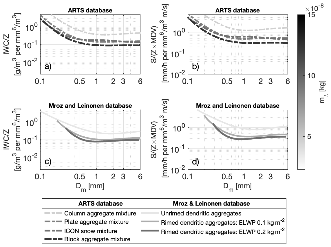
Figure 3 G-band simulations using exponential PSDs and different particle habits from the ARTS scattering database (Eriksson et al., 2018) (dashed lines in panels (a) and (b)) and the database of Mroz and Leinonen (2023) (solid lines in panels (c) and (d)). Panels (a) and (c) show the ratio $\mathrm{IWC}/Z$, and panels (b) and (d) show $S/(Z\times \mathrm{MDV})$ for a range of D_m. The lines are shaded in order of the m_λ values provided in Table 1, with darker shades representing larger m_λ.

By inspection of the simulation data we can estimate 𝒜 directly from the region of the $\mathrm{IWC}/Z$ curve where the values become nearly constant. In Fig. 3, we present simulations with the 7 different scattering models to show the effect of particle habit. This figure follows the same format as Figs. 1f and 2f. Figure 3a and b show results using the ARTS mixtures, and Fig. 3c and d use particles from the Mroz and Leinonen (2023) database. The shading of the lines was chosen based on the value of m_λ for each habit (see Table 1). The particles with smallest m_λ (i.e the unrimed dendritic aggregates) are plotted using the lightest shade of grey, with darker shades representing habits with increasing m_λ. It is clear that the different habits show similar qualitative behaviour, but different quantitative behaviour. The ratios are generally higher for lower mass particles, and lower for more massive particles. This suggests that m_λ is a key sensitivity for the method presented here. In other words, knowledge of m_λ is required in order to determine the magnitude of the asymptotic value. We note that for a given m_λ, the ratios are different between the two databases. Since oriented particles have their mass distributed more widely in the horizontal and more narrowly in the vertical compared to particles with random orientation, a particle of a given mass will exhibit less non-Rayleigh scattering if it is oriented. This results in increased c_f, thus increasing κ, as seen in Table 1.

Evidently, the curves are not perfectly flat. The plate and block aggregate mixtures from ARTS appear to approach an asymptotic limit more rapidly, whilst some of the others (such as the column aggregate mixture and the unrimed dendritic aggregates) show slight oscillations of $\mathrm{IWC}/Z$ and $S/(Z\times \mathrm{MDV})$ with D_m. In the following section, we hypothesise that this is related to the form of the function f, which captures the deviation from Rayleigh scattering, and in particular how closely f of the aggregate models follows the power law scaling assumed in Sect. 4.

Since, in practice, these curves are not perfectly flat, we choose a representative value at D_m=2 mm (i.e. centrally within the 1–3 mm interval used to estimate c_ns and $c_{R_{\mathrm{g}}}$, as discussed below) and tabulate this as 𝒜_IWC in Table 1.

For completeness, we also estimate the asymptotic value of $S/(Z\times \mathrm{MDV})$ which is tabulated as 𝒜_S. Since our figures have S in units of mm h⁻¹, 𝒜_S and 𝒜_IWC are not numerically equal, but should be trivially related to each other by a unit conversion, and indeed we find these two independent estimates are consistent to within 6 %.

To work out the dimensionless non-spherical scattering coefficient c_ns, we calculated Z at 3 GHz (i.e. in the Rayleigh regime) using an exponential PSD, and compared it to results calculated using Rayleigh spheres of the same mass (i.e. Eq. 7 with c_ns=1). Dividing the two quantities gives c_ns. This was repeated for PSDs with different D_m, and an average of the values obtained in the interval D_m=1–3 mm is shown in Table 1.

Estimation of $c_{R_{\mathrm{g}}}=R_{\mathrm{g}}/D$ is straightforward for the ARTS particles, since we have the full shape data of each particle, and from that we estimated R_g and D directly. Again, we computed a representative average value of this parameter. To do this, we first computed a mass-weighted average of $c_{R_{\mathrm{g}}}^{-b}$ across the particle size distribution, and then inverted the result to obtain an overall value of $c_{R_{\mathrm{g}}}$ for the complete distribution:

$$\begin{array}{}\text{(14)}& c_{R_{\mathrm{g}},m}={\left[{\displaystyle \frac{{\int }_{\mathrm{0}}^{\mathrm{\infty }}N\left(D\right)m\left(D\right)c_{R_{\mathrm{g}}}^{-b}\mathrm{d}D}{\mathrm{IWC}}}\right]}^{-\mathrm{1}/b}.\end{array}$$

Repeating this process for PSDs with D_m=1–3 mm as before, we took a median of the resulting values and this is the figure shown in Table 1. The rationale for averaging $c_{R_{\mathrm{g}},m}^{-b}$ is that the coefficient appears in this (nonlinear) form in κ. $c_{R_{\mathrm{g}},m}^{-b}={\int }_{\mathrm{0}}^{\mathrm{\infty }}N\left(D\right)m\left(D\right)c_{R_{\mathrm{g}}}^{-b}\mathrm{d}D/\mathrm{IWC}$. As for c_ns, we use the median value for D_m in the range 1–3 mm.

Since detailed shape data is not openly available for the particles from the database of Mroz and Leinonen (2023), $c_{R_{\mathrm{g}}}$ cannot be calculated in the same way for those particles. However, Leinonen and Szyrmer (2015) suggest that $c_{R_{\mathrm{g}}}\approx \mathrm{0.287}$, which is consistent with the values calculated for the ARTS particles, and this is the value we have used in our analysis.

After calculating c_ns and $c_{R_{\mathrm{g}}}$, the only unknown coefficient is c_f. To obtain c_f, we can use the asymptotic values of 𝒜 from our simulations, and divide this by the value of $\mathrm{1}/\mathit{\kappa }{m}_{\mathit{\lambda }}$ that would be obtained if c_f were equal to one. We used 𝒜_IWC to determine the value of c_f given in Table 1. This means calculating $\mathrm{1}/\mathit{\kappa }{m}_{\mathit{\lambda }}$ using κ and m_λ in the table is equivalent to 𝒜_IWC in the table (allowing for a unit conversion of 10³ to convert the SI units of IWC kg m⁻³ to the more convenient units of g m⁻³ used in Figs. 1 and 3).

The values of c_ns and $c_{R_{\mathrm{g}}}$ are quite consistent across the various particle models, with values lying in the ranges 1.16±6 % and 0.31±10 % respectively. There is a higher variation (factor of 3.2) in c_f. However the values are fairly consistent for the ARTS habits with values of 1.15–1.58, while the majority of the variation in c_f comes from the particles in the rimed database. A larger value of c_f=2.49 is found for the unrimed dendritic aggregates, and the largest value of c_f=3.71 is found for rimed dendritic aggregates with ELWP = 0.1 kg m⁻². As riming increases to ELWP = 0.2 kg m⁻², c_f decreases to 1.92.

The coefficients are used to calculate κ in Table 1, which is found to be very similar for all four ARTS mixtures considered, varying by only 25 %. However, m_λ varies by a factor close to 4 for these mixtures. This implies that in some cases it may be suitable to assume a value for κ, meaning the only thing we need to know is m_λ. In other words, we don't need to assume a particular scattering model, the only parameter required to perform a retrieval is the mass of a wavelength-sized particle. There is greater variability in κ for the particles from the rimed database. Considering all seven particle habits used here, κ varies by a factor of 3 (which is likely to be driven by the large variation in c_f since the variability is small for the other coefficients). However m_λ varies more strongly, by a factor of 6.5. Thus we suggest that m_λ is the primary sensitivity in controlling what 𝒜 is.

6 Testing the assumed power-law scaling of the non-Rayleigh scattering (f)

As discussed in Sect. 4, Sorensen (2001) used RGA to demonstrate that for fractal aggregates large enough compared to the wavelength (i.e. $\frac{\mathrm{4}\mathit{\pi }{R}_{\mathrm{g}}}{\mathit{\lambda }}\gtrsim \mathrm{1}$), f is characterised by the power law given in Eq. (10). We now test in more detail whether that approximation holds for realistic ice particle models from the scattering databases. The data in both databases were calculated using the numerically exact discrete dipole approximation. Provided the resolution of the discretisation is sufficient, the DDA provides an accurate solution to Maxwell's equations (Yurkin and Hoekstra, 2007).

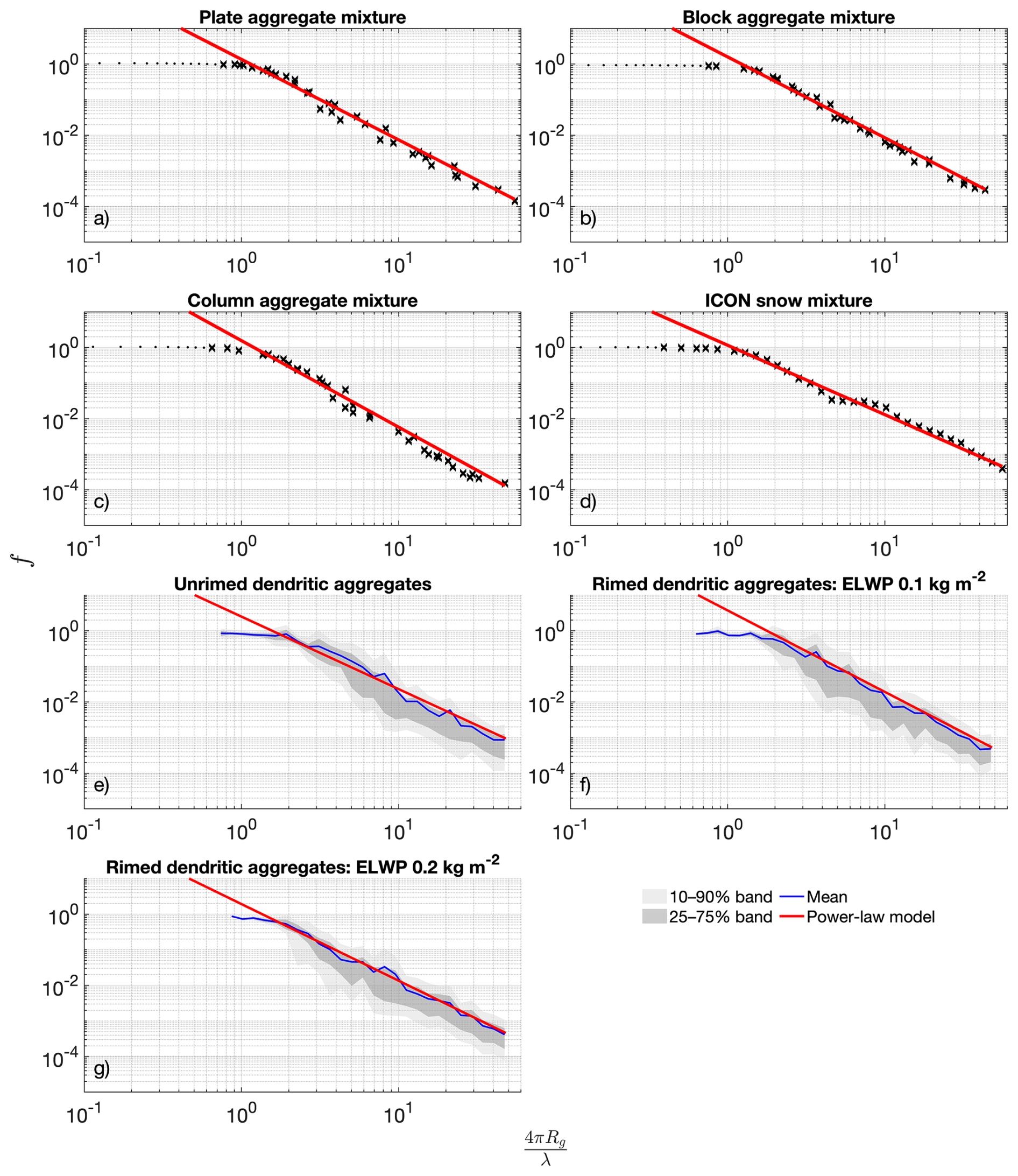
Figure 4 Comparison of f as a function of $\frac{\mathrm{4}\mathit{\pi }{R}_{\mathrm{g}}}{\mathit{\lambda }}$ for the particle habits used in this study. Panels (a)–(d) show results for the ARTS mixtures: black dots and crosses represent monomers and aggregates, respectively, with f computed using Eq. (15). Panels (e)–(g) summarise aggregates from the rimed database. For each logarithmic bin in $x=\frac{\mathrm{4}\mathit{\pi }{R}_{\mathrm{g}}}{\mathit{\lambda }}$, a kernel density estimate of log ₁₀f is used to obtain smooth quantiles. The light grey band shows the 10 %–90 % range, the darker band shows the interquartile range, and the blue line shows the mean. Red lines in all panels show the theoretical power-law expression (Eq. 10), which captures the scaling for $\frac{\mathrm{4}\mathit{\pi }{R}_{\mathrm{g}}}{\mathit{\lambda }}⪆\mathrm{1}$. For the ARTS particles, R_g is computed directly for each particle; for the Mroz and Leinonen (2023) database we use R_g≈0.287D (Table 1).

The red lines in Fig. 4 show f computed using Eq. (10), for the particle habits outlined in Table 1. From the equations outlined in Sect. 4, we can write the non-Rayleigh radar cross section as:

$$\begin{array}{}\text{(15)}& {\mathit{\sigma }}_{\mathrm{r}}=\mathrm{36}{\mathit{\pi }}^{\mathrm{3}}{\mathit{\lambda }}^{-\mathrm{4}}{\displaystyle \frac{m^{\mathrm{2}}}{{\mathit{\rho }}_{\mathrm{ice}}^{\mathrm{2}}}}{\left|{\displaystyle \frac{\mathit{ϵ}-\mathrm{1}}{\mathit{ϵ}+\mathrm{2}}}\right|}^{\mathrm{2}}{c}_{\mathrm{ns}}f.\end{array}$$

Thus we may also calculate f for realistic ice particle models by using σ_r and m from the databases, and c_ns from Table 1. Figure 4 shows f as a function of $\frac{\mathrm{4}\mathit{\pi }{R}_{\mathrm{g}}}{\mathit{\lambda }}$, computed for the various particles in this study. In Fig. 4a–d, dots correspond to monomers from each ARTS mixture and crosses to the associated aggregates. At small values of $\frac{\mathrm{4}\mathit{\pi }{R}_{\mathrm{g}}}{\mathit{\lambda }}$, f≈1 and these particles correspond to the monomer habits in the mixture, along with some of the smaller aggregates. The crossover to power law scaling for f begins at $\frac{\mathrm{4}\mathit{\pi }{R}_{\mathrm{g}}}{\mathit{\lambda }}\approx \mathrm{1}$ for each of the ARTS habits, following the expected behaviour of Sorensen (2001). Figure 4e–g summarise the aggregates from the Mroz and Leinonen (2023) rimed database using statistical envelopes rather than individual symbols. For each logarithmic bin in $\frac{\mathrm{4}\mathit{\pi }{R}_{\mathrm{g}}}{\mathit{\lambda }}$, a kernel density estimate of log ₁₀f is used to derive smooth quantiles, which are shown as grey shaded bands, with the mean shown by the blue line. These panels reveal similar overall behaviour to the ARTS mixtures, but the crossover to power law scaling occurs at slightly larger values closer to 2. This shows that power law scaling is indeed evident in the scattering data for complex aggregates, rimed and unrimed, in the G-band, validating a cornerstone of our theoretical interpretation. Using the values of $c_{R_{\mathrm{g}}}$ in Table 1, we can see that the point where the crossover to power law scaling begins corresponds to $D\approx \mathit{\lambda }/\mathrm{4}$, at which size scattering from ice at the front and back of the particle would be out of phase in the backward direction. At 200 GHz (λ=1.5 mm) this critical diameter is 0.375 mm.

As outlined in Sect. 4, the power law scaling of f led to the results in Eqs. (12) and (13), whereby an almost direct proportionality between Z and IWC, and Z×MDV and S was deduced. In other words, the power law scaling of f drives the flattening of the ratios $\mathrm{IWC}/Z$ and $S/(Z\times \mathrm{MDV})$ in the G-band. Although we determined in the previous section that m_λ is the key parameter to determine the magnitude of the asymptotic value, the power-law behaviour of f is the factor which drives the flattening of $\mathrm{IWC}/Z$ in the first place. This influence is evident when comparing the data in Figs. 4 to 3. In Fig. 4, the data for the block and plate aggregate mixtures closely match the power law, and the ratios in Fig. 3 are the flattest for these habits. For example, in the range D_m=1–6 mm, the $\mathrm{IWC}/Z$ ratio varies by only 3 % and 11 % for the blocks and plates, while there are larger, more systematic deviations from the idealised power law curve for the large column aggregate mixture and the ICON snow mixture, resulting in larger variations in $\mathrm{IWC}/Z$ of 26 % and 27 %. The power law generally overestimates the column aggregate mixture data at larger values of $\frac{\mathrm{4}\mathit{\pi }{R}_{\mathrm{g}}}{\mathit{\lambda }}$. For the ICON snow mixture, the power law underestimates the data at $\frac{\mathrm{4}\mathit{\pi }{R}_{\mathrm{g}}}{\mathit{\lambda }}=\mathrm{1.5}$, overestimates it at $\frac{\mathrm{4}\mathit{\pi }{R}_{\mathrm{g}}}{\mathit{\lambda }}=\mathrm{4.5}$, and underestimates it again around $\frac{\mathrm{4}\mathit{\pi }{R}_{\mathrm{g}}}{\mathit{\lambda }}=\mathrm{10}$. Because λ is fixed, and R_g∝D, these under/overestimations feed through to the scattering properties of different particle sizes, and as D_m is varied, these particle sizes are weighted to a greater or lesser extent in the value of Z and MDV, producing weak oscillations around the anticipated constant value of $\mathrm{IWC}/Z$ and $S/(Z\times \mathrm{MDV})$.

7 Sensitivity to the form of the particle size distribution (PSD)

Analysis of in-situ observations has generally led to cloud PSDs being parameterised by either exponential or gamma distributions e.g. Sekhon and Srivastava (1970) and Heymsfield et al. (2002, 2013). In this subsection, we consider the effect of PSD shape on our results. So far, we have assumed an exponential distribution shape. To investigate the sensitivity to this assumption, G-band simulations for plate aggregates are repeated using gamma PSDs $N\left(D\right)=N_{\mathrm{0}}{D}^{\mathit{\mu }}\exp (-\mathrm{\Lambda }D)$, where μ is a shape parameter. If μ=0, the gamma PSD reduces to an exponential PSD, while increasing μ decreases the small particle concentration, and produces a less disperse distribution. Negative values of μ are also possible, which give very broad distributions, including large numbers of small particles. Care is required when μ<0 since some moments of the distribution can become divergent – this is not the case for IWC, S or Z in the $\mathit{\mu }=-\mathrm{1}$ case shown here. The different coloured lines in Fig. 5 show results for representative values of μ, ranging from −1 to 5 (based on the analysis in Mason et al., 2019). Figure 5a and b show the ratios $\mathrm{IWC}/Z$ and $S/(Z\times \mathrm{MDV})$ for a range of D_m. Furthermore, Fig. 5c and d show the percentage difference of the ratios for nonzero μ values relative to our nominal simulations at μ=0 from Figs. 1 and 2.

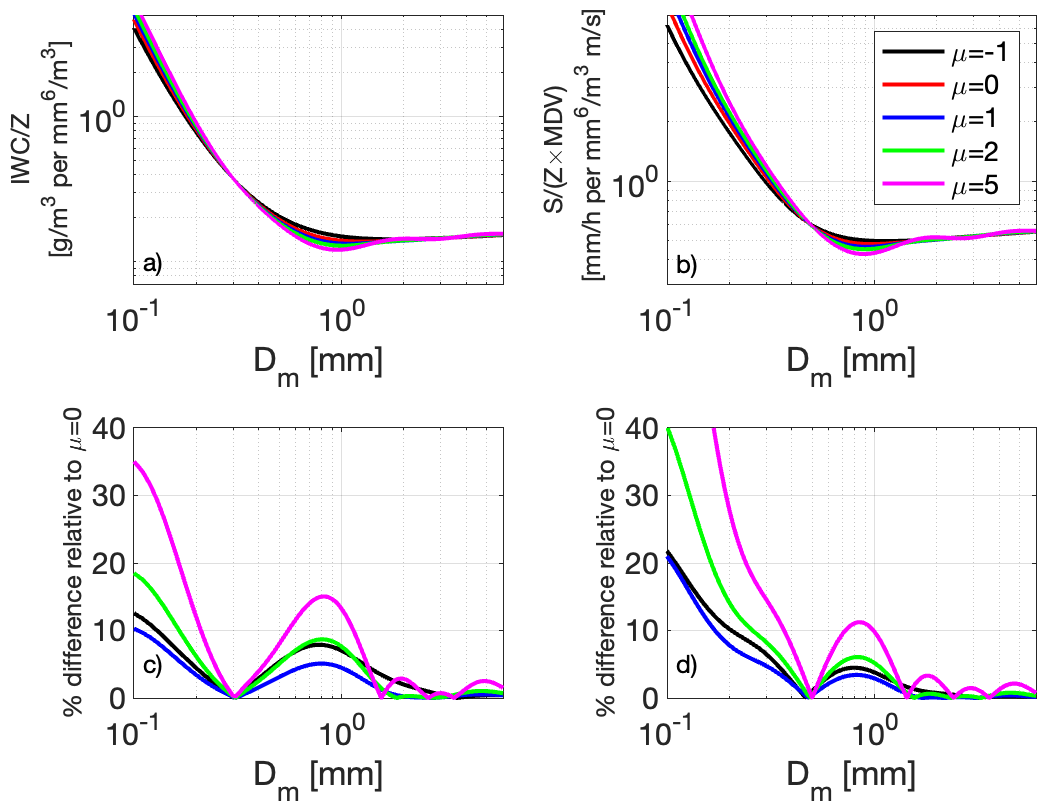
Figure 5 G-band simulations using the plate aggregate mixture and gamma PSDs. Panels (a) and (b) show the $\mathrm{IWC}/Z$ and $S/(Z\times \mathrm{MDV})$ ratios for a range of D_m. The different line colours correspond to different values of the shape parameter μ, where μ=0 (red lines) is equivalent to an exponential PSD. Panels (c) and (d) show the percentage difference relative to the μ=0 case.

It is clear that in the region of D_m we are interested in, the results are not very sensitive to the PSD shape parameter. Varying μ between −1 and 2 causes differences of less than 9 % for IWC, and less than 6 % for S, relative to using an exponential distribution. The differences are higher, with more oscillatory behaviour, for the largest value of μ (5), but remain below 12 %. This weak oscillatory variation is likely because as μ increases, the PSD becomes increasingly narrow, and dominated by a more restricted range of particle size. The scattering model comprises a single particle per size bin, and for this situation these will be aggregates of varying (random) configurations. The scattering properties fluctuate with size as a result of the random realisations, and the integrated values at high μ are more sensitive to these fluctuations, because of the narrower weighting in D space. In nature, these fluctuations may not be evident, because natural clouds probed by radar consist of an enormous ensemble of particles at all sizes. We therefore suspect this sensitivity to μ is an upper limit to the true sensitivity to PSD shape.

At very small D_m (below 0.3 mm) there is stronger sensitivity to the PSD shape, as the scattering becomes increasingly influenced by smaller particles in the Rayleigh regime. However, since our target in this work is D_m>0.5 mm, this is not a concern.

8 Application to case studies

To illustrate the practicalities of retrieving IWC and S using Eqs. (12) and (13), we now present measurements of two ice-phase clouds which passed over the Chilbolton Observatory in the UK, using the GRaCE 200 GHz cloud radar. This instrument has a 0.1° vertically-pointing beam, transmits around 80 mW output power in a pulse of variable duration, and records full Doppler spectra profiles, which can then be analysed to estimate Z and MDV. Further details can be found in Courtier et al. (2022). The aim of this section is to (a) demonstrate how retrievals can be made in practice, and (b) to provide some in-situ evidence (from a precipitation gauge in Case 1, and aircraft measurements in Case 2) that the S and IWC retrievals produced are realistic.

8.1 Attenuation

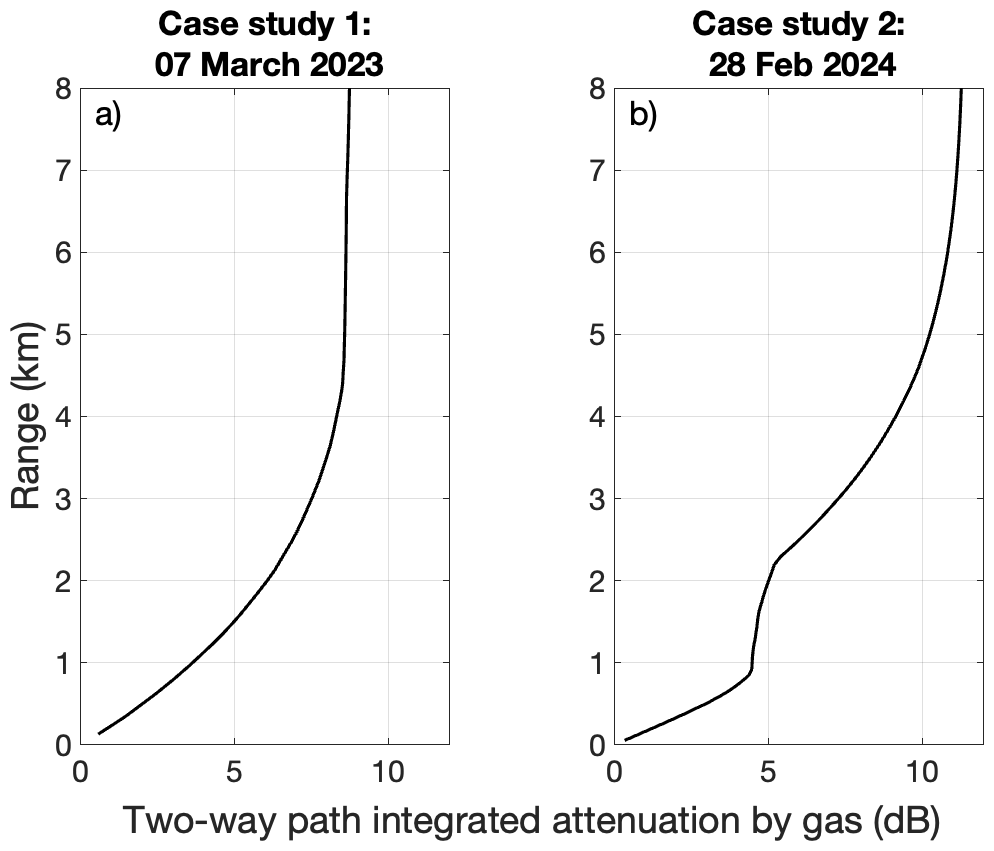
Attenuation is very important at G-band (Battaglia et al., 2014). In what follows, reflectivity data has been corrected for water vapour attenuation using the absorption model of Liebe (1989), along with nearby soundings at Larkhill (approximately 30 km from Chilbolton; Case 1) and a dropsonde released at 11 : 22 (<10 km from Chilbolton; Case 2). The vapour attenuation profiles are shown in Fig. 6.

Figure 6 Two-way path integrated attenuation by water vapour in the G-band calculated using the absorption model of Liebe (1989) and soundings from Larkhill on (a) 7 March 2023, and (b) 28 February 2024.

Attenuation by ice particles in the cloud is much smaller than from water vapour, but not completely negligible. Figure 7a shows a relationship between attenuation in the G-band and reflectivity at Ka-band, derived from simulations using the particle models in this study (see Appendix A). The advantages of using the Ka-band reflectivity as a variable to diagnose attenuation is the fact that there is significantly less attenuation from all sources (vapour, ice, liquid water) than there is in the higher frequency bands, so the value of Z that is measured at Ka-band is the true reflectivity of the particles at that frequency. In the cases presented here, Ka-band data from the Copernicus 35 GHz cloud radar with a 0.25° vertically-pointing beam was also available (Walden, 2025). This allows us to diagnose attenuation by ice using the relationship shown in Fig. 7a, which is used to correct the G-band reflectivity data. In Case 1, the estimated two-way path integrated attenuation by ice at 4 km ranges from values < 0.1 to about 4.8 dB, with an average correction throughout the day of around 1.4 dB. In Case 2, the path integrated attenuation at 8 km is less variable throughout the day, ranging from 0.6–2.6 dB, while the average correction is similar to Case 1, at 1.3 dB.

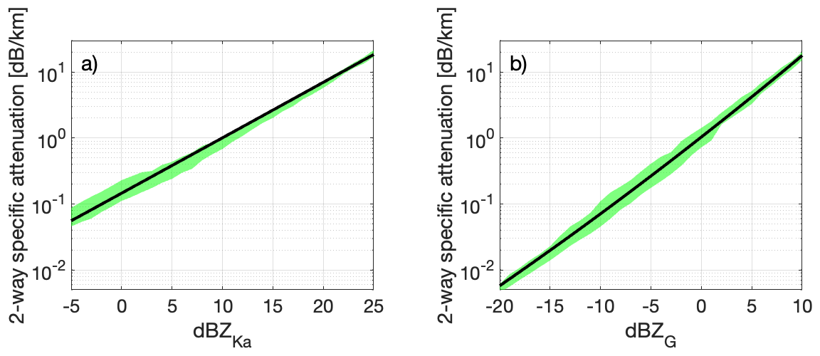
Figure 7 Panel (a) shows the relationship derived between dBZ_Ka and attenuation by ice in the G-band. We used this relationship to correct for attenuation by ice in the data presented here. Panel (b) shows a fit derived in the same way, but with dBZ_G on the x-axis. Note that the x-axis limits in panels (a) and (b) are different. The green shaded regions show the interquartile range of the data, representing variations due to differences in the scattering model and PSDs.

Since the ideas presented in this manuscript could, in principle, be applied when only a single frequency is available, Fig. 7b shows the same relationship but now correlating attenuation at G-band with unattenuated reflectivity at G-band. Application of this second relationship is more complicated, because it requires the unattenuated reflectivity to be estimated. One approach might be to correct the reflectivity from the surface upward, moving range gate by gate. We include this information for completeness, but in what follows we will apply ice attenuation corrections based on the Ka-band profile measured at the same time.

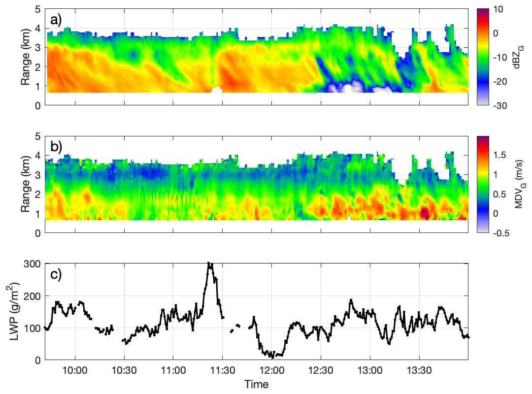
Figure 8 Panels (a) and (b) show dBZ and MDV measured by the GRaCE G-band radar at Chilbolton observatory on 7 March 2023. The liquid water path (LWP) retrieved from a collocated RPG HATPRO-G5 microwave radiometer (Humidity And Temperature PROfiler; Walden, 2024a), using the instrument's software, is shown in panel (c).

Supercooled liquid water is also a significant source of attenuation at G-band (Battaglia et al., 2014). In Case 2 there is no evidence of significant liquid water. In Case 1, retrievals from a collocated RPG HATPRO-G5 microwave radiometer (Humidity And Temperature PROfiler; Walden, 2024a), using the instrument's software, suggest that the liquid water path is typically between 50 to 200 g m⁻² (Fig. 8c). This corresponds to a total 2-way attenuation through the cloud of approximately 1 to 4 dB in the G-band. In what follows we do not attempt to correct for this, which may lead to underestimation of IWC and S in the upper portions of the cloud system. However, the key data of interest for our analysis is in the lower parts of the cloud (near 1 km height), where the attenuation is likely to be smaller, and the agreement with gauge data in Case 1 suggests that this is not a major effect, particularly given the uncertainties inherent in comparing gauge data from the surface with radar data aloft.

8.2 Case study 1: 7 March 2023

On 7 March 2023 a shallow snow band passed over the observatory, and was sampled by the GRaCE radar. This case study is analysed in more detail in McCusker et al. (2025), which includes a dual-frequency retrieval of D_m, indicating that almost everywhere in the cloud field has D_m>0.5 mm. This is therefore an appropriate target for our retrieval method.

Panels (a) and (b) of Fig. 8 show dBZ and MDV measured by the GRaCE G-band radar over a 4 h period. During this time both the cloud depth (4 km) and liquid water path (∼ 100 g m⁻²) were reasonably consistent, albeit with some localised fluctuations in both quantities. After 14:00 UTC the cloud became increasingly shallow and broken, with larger, more variable liquid water path. During the 4 h window presented here, the majority of the reflectivity values lie in the range −10 to 0 dBZ. Doppler velocities are typically around 0.3 m s⁻¹ at 3 km (positive velocity is downward), increasing in magnitude at lower altitudes to around 0.7–1.5 m s⁻¹ at 1 km.

There were no airborne in-situ cloud measurements collected on this day, so cloud particle imagery is not available to constrain the choice of scattering model. However, McCusker et al. (2025) examined the Doppler spectra for this case study. Through analysis of triple frequency diagrams in spectral space, they concluded that the measurements were consistent with the Mroz and Leinonen (2023) rimed snowflakes. Taking this as guidance, and acknowledging that in Fig. 8c the liquid water path (LWP) oscillates around 0.1 kg m⁻², we use the rimed dendritic aggregates with ELWP 0.1 kg m⁻² from Table 1 for the retrieval. Using these values we simply compute $\mathrm{IWC}=Z\times {\mathcal{A}}_{\mathrm{IWC}}$ and $S=Z\times \mathrm{MDV}\times {\mathcal{A}}_S$.

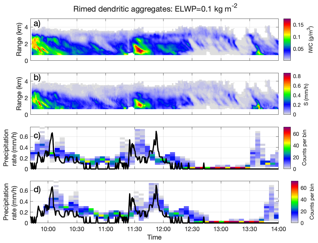
Figure 9 Panels (a) and (b) show IWC and S retrieved from the measured Z and MDV on 7 March 2023 shown in Fig. 8 using 𝒜_IWC and 𝒜_S estimated from the simulations for rimed dendritic aggregates with ELWP = 0.1 kg m⁻². The coloured histogram data in panels (c) and (d) show the values of retrieved S from the bottom ∼ 500 m of cloud. Overlaid on the histograms is a black line showing the 1 min moving average precipitation rate measured from a drop counting rain gauge at Chilbolton. In panel (d) the histogram data has been shifted in time by 14.5 min to account for the approximate time it may take for precipitation to reach the rain gauge at the ground.

The resulting IWC and S values are shown in panels (a) and (b) of Fig. 9. Under the assumption of rimed dendritic aggregates, the retrieved IWC is typically a few hundredths of a gram per cubic metre, with a few isolated fallstreaks of larger IWC values reaching 0.17 g m⁻³. Light snowfall rates with values of S generally less than 0.3 mm h⁻¹ are retrieved, with some isolated streaks producing higher values around 0.6 mm h⁻¹.

To assess the realism of the retrieved fields, we have compared the snowfall rate retrieved in the lower parts of the cloud (we use the lowest ∼ 500 m of available data) to a fast response precipitation gauge at the ground (Norbury and White, 1971). The sounding from Larkhill indicates that the 0 °C wet-bulb isotherm is around 100 m above the surface on this day, so the snowflakes are likely to have at least partially melted by the time they reach the gauge funnel. The results are shown in Fig. 9c and d. The colours are time series of the histogram of S retrieved from the radar aloft over the 500 m deep layer. The black line in each panel displays the precipitation rate from the gauge, showing measurements of light precipitation. In Fig. 9c it is clear that peaks in the precipitation rate at the ground are measured at a later time than when peaks in S are retrieved in the lower cloud regions. This corresponds to the time taken for particles in this region to reach the ground. In Fig. 9d we account for a time delay by shifting the histogram data in time by 14.5 min. This corresponds to particles in the 500 m deep layer falling at approximately 0.8–1.3 m s⁻¹. Qualitatively, the histogram of retrieved S displays similar behaviour to the rain gauge measurements. At times of higher precipitation rate, the location and magnitude of the peaks are captured quite accurately in the retrieval. At times of low precipitation rate, the values of retrieved S are slightly larger than observed by the gauge. This could be the result of evaporation, or variations in the properties of the particles in time (for example the mass-size relationship may change as the amount of riming varies). Towards the end of the time series, there is a peak in retrieved S that is not reflected in the gauge measurements. This discrepancy is likely due to the narrow, small-scale nature of the feature, as evident in panels (a) and (b) of Fig. 8. The retrieval represents conditions approximately 1 km above the surface, and we are assuming vertical precipitation when performing a comparison with measurements at the surface. However, in reality, horizontal advection or wind drift may cause the precipitation to fall outside the gauge's catchment area, leading to a lower recorded value at the surface. This highlights the strength of radar-derived snowfall rates in resolving localised precipitation that surface gauges may fail to detect.

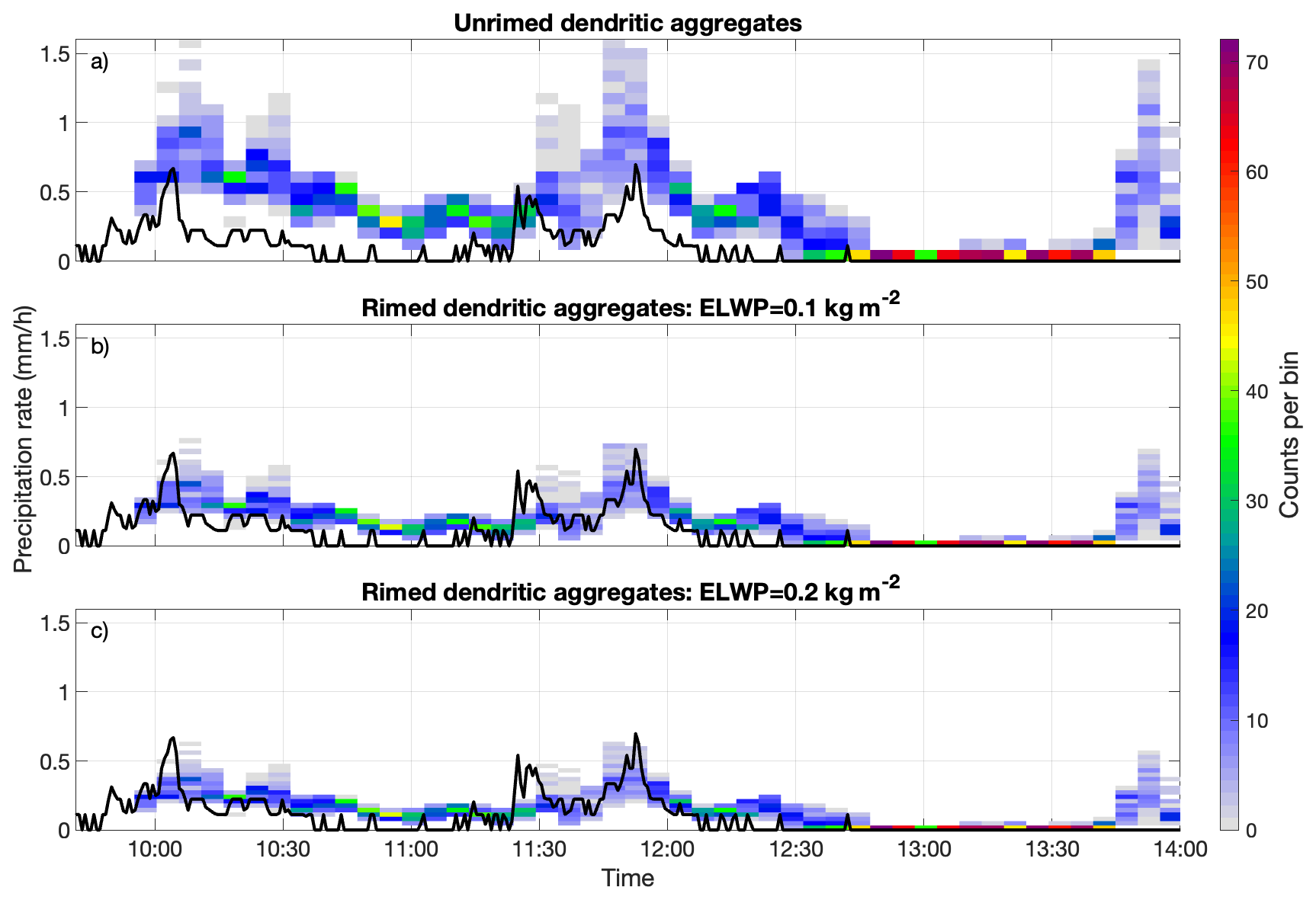
Figure 10 Sensitivity of S retrievals to the choice of particle habit. As in Fig. 9d, the histograms show S retrieved from the bottom ∼ 500 m of cloud, while the black lines show the 1 min moving average precipitation rate measured from a drop counting rain gauge at Chilbolton. Panels (a)–(c) show results using the three particle habits from the database of Mroz and Leinonen (2023). Panel (a) uses unrimed dendritic aggregates, panel (b) uses rimed dendritic aggregates with ELWP = 0.1 kg m⁻² (i.e. the original result in Fig. 9d), and panel (c) uses rimed dendritic aggregates with ELWP = 0.2 kg m⁻².

To assess the sensitivity of our results to the choice of particle model, we repeat the analysis from Fig. 9 using different scattering assumptions (Fig. 10). Figure 10b shows the original result obtained using rimed dendritic aggregates with an ELWP of 0.1 kg m⁻². For comparison, Fig. 10a uses unrimed dendritic aggregates (i.e., lower-mass particles), while Fig. 10c uses rimed aggregates with a higher ELWP of 0.2 kg m⁻². The use of unrimed particles results in larger retrieved values of S, approximately doubling compared to the baseline in Fig. 10b. In contrast, increasing the riming from ELWP = 0.1 to 0.2 kg m⁻² yields only a modest reduction in S of about 0.1 mm h⁻¹, corresponding to a difference of roughly 20 % between the two rimed models. These results reflect the differences in 𝒜_S values in Table 1, which vary more substantially between the unrimed and rimed models, but remain similar for the two rimed models.

8.3 Case study 2: 28 February 2024

The GRaCE G-band radar also collected measurements from Chilbolton on 28 February 2024. The Facility for Airborne Atmospheric Measurements (FAAM) BAe-146 research aircraft (http://www.faam.ac.uk, last access: 17 December 2025) performed a flight on this day (C374), operating as part of the Characterising CirRus and icE cloud acrosS the specTrum-Microwave (CCREST-M) project. This provided a unique opportunity to collect G-band radar measurements from GRaCE along with sampling in-situ microphysics almost coincidentally.

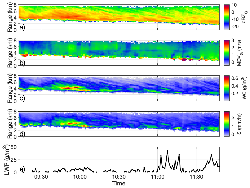
Figure 11 Panels (a) and (b) show dBZ and MDV measured by the GRaCE G-band radar at Chilbolton observatory on 28 February 2024, while panels (c) and (d) show retrieved IWC and S. The retrievals assume that $\mathit{\kappa }=\mathrm{7}\times {\mathrm{10}}^{\mathrm{10}}$ mm⁶ kg⁻², and m_λ is calculated using the Brown and Francis (1995) mass-size relationship. Panel (e) shows the LWP retrieved from the RPG HATPRO-G5 microwave radiometer, using the MWRpy software (Walden, 2024b).

GRaCE collected observations of cloud associated with an approaching warm front. The system eventually brought rain which attenuated the G-band signal. We focus on the deep stratiform ice cloud ahead of the surface rainfall. Panels (a) and (b) of Fig. 11 show dBZ and MDV from 09:12–11:48 UTC. Lidar data collected from the Vaisala CL51 instrument (Walden, 2024c) during this case study revealed some low-level liquid cloud beneath the ice cloud, at a height of approximately 0.3–0.6 km. The total 2-way attenuation by the liquid cloud was calculated using the LWP retrieved from the RPG HATPRO-G5 microwave radiometer using the MWRpy software (Walden, 2024b; Fig. 11e), and the reflectivity values from the ice cloud have been corrected based on those estimates. Similar to the first case study, the reflectivity values in Fig. 11a typically range from around −10 to 0 dBZ. As well as a systematic trend for higher reflectivities at lower altitude, fall streaks are also apparent in the data indicating significant horizontal variability within the cloud. Doppler velocities mainly range from ≈0.5 to 1.2 m s⁻¹.

As discussed in previous sections, m_λ is the key sensitivity for the method presented here. From Table 1, it can be seen that for the ARTS aggregate mixtures, $\mathit{\kappa }\approx (\mathrm{7}\pm \mathrm{1})\times {\mathrm{10}}^{\mathrm{10}}$ mm⁶ kg⁻². Thus, in many cases where the cloud particles are mixtures of unrimed pristine crystals and aggregates, one could set $\mathit{\kappa }=\mathrm{7}\times {\mathrm{10}}^{\mathrm{10}}$ mm⁶ kg⁻² and calculate m_λ using a pre-defined mass-size relationship, such as the one given by Brown and Francis (1995). This eliminates the requirement of a specific particle habit assumption. Since the particle imagery shows that the dominant crystal habits throughout this case study were unrimed bullet rosettes and columns, along with relatively small aggregates of those habits (see CIP-15 imagery in Fig. 12), we believe this is a suitable method to use here. Using the Brown and Francis (1995) mass-size relationship corresponding to D (as presented in Hogan et al., 2012) results in a value of $\mathcal{A}=\mathrm{1}/\mathit{\kappa }{m}_{\mathit{\lambda }}=\mathrm{2.8}\times {\mathrm{10}}^{-\mathrm{1}}$ g mm⁻⁶. This value of 𝒜 is used to convert measurements of Z and MDV to IWC and S (IWC [g m⁻³] = Z×𝒜; S[mm h⁻¹] = $Z\times \mathrm{MDV}\times \mathcal{A}\times \mathrm{3.6}$). These are shown in panels (c) and (d) of Fig. 11. The retrieved ice water content varies from a few hundredths of a gram per cubic metre up to around 0.6 g m⁻³ in certain regions of the cloud (4.5 km, 09:50 UTC). The snowfall rate has a similar dynamic range, with rates of a few tenths of a millimetre per hour up to a peak of ≈2.5 mm h⁻¹.

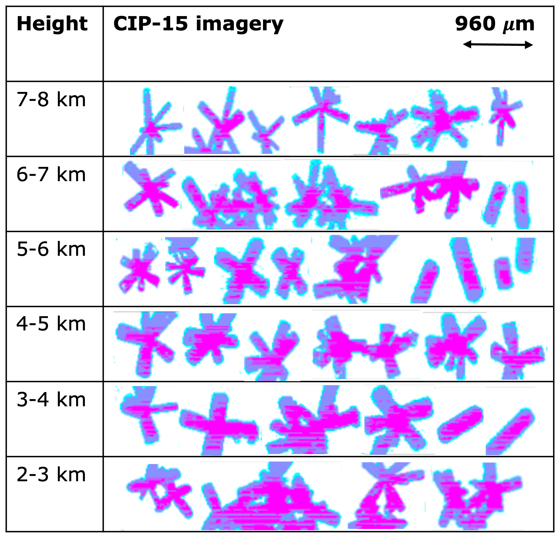
Figure 12 Examples of CIP-15 imagery at different heights on 28 February 2024. The pixel resolution is 15 µm. The imagery is displayed using three different colours to represent different levels of light intensity reduction at the detector: cyan (25 %), blue (50 %), and magenta (75 %).

In Fig. 13 we plot the IWC estimates from the G-band radar as a 2D probability histogram. The black line overlaid on the histogram shows a profile of IWC estimated using measurements of the liquid and total water (ice plus liquid) contents from the Nevzorov probe, which is accurate to within about 0.002 g m⁻³ (see Abel et al., 2014 for a description of the probe on the FAAM BAe-146 research aircraft). The aircraft performed a stepped descent through the cloud and we use data collected between 11:18–12:48 UTC in order to obtain an IWC profile throughout the entire height range. The profile was constructed by averaging Nevzorov IWC measurements collected at different altitudes during this time into 90 m range bins to match the range resolution of GRaCE on that day. The grey shaded region shows the range of values measured in each 90 m altitude bin, with the differences resulting from cloud inhomogenity. The red line overlaid on the histogram shows a profile of IWC obtained from integrating the PSD measured with the CIP-15 and CIP-100 probes during the aircraft descent, assuming the Brown and Francis (1995) mass-size relationship. As with the Nevzorov data, the shading indicates the range of values within each bin. This shows that the Brown and Francis (1995) relationship is generally consistent with the aircraft measurements. However, between about 4.8–6 km, the CIP IWC is lower than the Nevzorov IWC, indicating that particles in this region may have a higher mass than what is predicted by the Brown and Francis (1995) relationship.

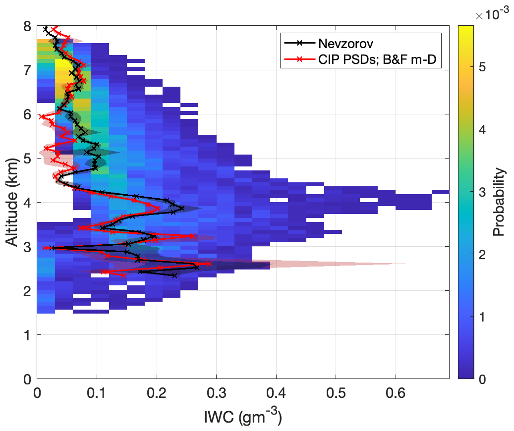
Figure 13 Probability histogram of retrieved IWC from dBZ_G, using $\mathit{\kappa }=\mathrm{7}\times {\mathrm{10}}^{\mathrm{10}}$ mm⁶ kg⁻² and m_λ from the mass-size relationship of Brown and Francis (1995). The black line shows the measured IWC profile using the Nevzorov probe on board the FAAM aircraft. The red line shows the IWC obtained from integrating the PSD measured with the CIP probes, assuming the Brown and Francis (1995) mass-size relationship. Both IWC profiles are averaged into 90 m range bins to match the range resolution of GRaCE, but shaded regions are included to show the range of values measured in each altitude bin.

We also estimated D_m using the CIP PSD data, which was found to be >0.5 mm at ranges of 7 km and below. Thus we expect the retrieval to be applicable to the majority of this cloud. D_m<0.5 mm at the very top of the cloud (higher than 7 km), so we may expect the retrieval to have lower accuracy in this region.

This comparison allows us to test the realism of the retrieval using the in-situ data, but the colocation of the two datasets in time and space is imperfect since the radar data shown were collected during the time period 09:12–11:48 UTC, while the IWC data were collected between 11:18–12:48 UTC. Moreover the radar was sampling vertical profiles at Chilbolton, while the aircraft sampled along a 120 km long radial extended out to the southwest of Chilbolton. As a result, only a statistical comparison is possible. Figure 13 shows that the Nevzorov IWC profile falls within the distribution of the retrieved values (with the exception of a shallow layer near 4.5 km height). Above 5 km the aircraft profile follows the peak of the radar distribution to within ≈ 0.03 g m⁻³. At lower altitudes the IWC profile from the aircraft shows large non-monotonic variations with height, which suggests there is significant inhomogeneity in the cloud. Despite these large fluctuations, the data still appear to fluctuate around the centre of the distribution of the radar retrievals. Overall, this comparison gives us further confidence that the method we are investigating in this paper produces realistic results.

9 Discussion and conclusions

In this study, we demonstrate, for the first time, the near-linear relationship between G-band radar reflectivity and ice water content, leveraging the strong non-Rayleigh scattering characteristics unique to these frequencies. This simplifies retrieval methods significantly compared to lower-frequency radars. We explore the strong non-Rayleigh scattering produced by ice particles in the G-band, and present theory and simulations to show that measurements of Z and Z×MDV are almost directly proportional to IWC and S, respectively. This is in stark contrast to the behaviour that occurs at lower frequencies, and presents the opportunity for simple but accurate retrievals of cloud ice quantities. In principle, these retrievals could take place using G-band measurements alone, provided the profiles can be corrected for attenuation by water vapour (the dominant component), liquid water (if present) and ice. Alternatively the approach here can be incorporated into a more sophisticated multi-frequency retrieval. One approach would be to use the simple Z–IWC relationship as a robust first estimate of the water content profile, which is subsequently refined using the dual frequency ratio data.

We provide theoretical background and analysis to show that the near constant values of $\mathrm{IWC}/Z$ and $S/(Z\times \mathrm{MDV})$ are expected for fractal aggregates that are large compared to the wavelength. The behaviour is driven by the power law scaling of f, the dimensionless factor used to express non-Rayleigh scattering behaviour, and is consistent with the analysis of Sorensen (2001). Since this latter behaviour was originally derived using RGA (which, as McCusker et al., 2019 and others have shown, does not capture the full physics of the scattering process), and since radar measurements of ice particles were not the intended application of Sorensen's study, it is necessary to turn to DDA scattering data on realistic ice particles to evaluate whether the anticipated scaling holds for real snowflakes. The simulations show that the power law scaling is indeed evident, and the expected linear relationship between IWC and Z is obtained. Some small fluctuations around this linear relationship are present (which are more evident when visualising their ratio as a function of D_m in Figs. 1 and 3). Digging into the details on the non-Rayleigh function f indicates that this fluctuation is driven by deviations from the overall power law scaling of f. We speculate that these deviations are driven by variability in the particle geometry (e.g. different random realisations of aggregates) for different particle sizes. The direct proportionality of IWC and Z is most accurate when f of the assumed particle model closely follows this assumed power law scaling.

The expected magnitude, 𝒜, of the asymptotic value of $\mathrm{IWC}/Z$ is dependent on κ and m_λ, but crucially is not sensitive to PSD parameters, and we show that the dominant factor controlling the magnitude of 𝒜 is m_λ, i.e. the mass of a wavelength-sized ice particle. If m_λ is known (i.e. we can place a constraint on the mass-size relationship), then we expect retrievals to have uncertainties within $\approx \pm \mathrm{30}$ % for IWC, and within ±15 % for S. These uncertainties become even narrower for D_m≳0.8 mm. The variability of κ between different particle scattering models is significantly smaller than the variability of m_λ, varying by only 25 % for the four unrimed particle mixtures from the ARTS database. In contrast, m_λ varies by a factor of almost 4 between the ARTS models. This suggests that it may be acceptable to fix the value of κ, leaving m_λ as the only free parameter to select in the retrieval method. This in turn would mean there is no requirement to base the retrieval on the existing scattering database particle models - instead it is sufficient to know m_λ from an appropriate mass-size relationship. We note that the unrimed and rimed dendritic aggregates from the database of Mroz and Leinonen (2023) have larger values of κ, which we propose is caused by the increase in c_f resulting from particle orientation. However, κ for all seven particle models considered here varies by a factor of 3, which is still considerably less than the factor of 6.5 variability in m_λ. In the future, we plan to examine the behaviour of different particle models and test the overall variability in κ and other parameters. Such an analysis would benefit from the availability of additional scattering data in the G-band.

The method is applicable in the regime where particles dominating the radar measurements are comparable to or larger than a quarter of a wavelength, and our data indicates this is satisfied for clouds where D_m⪆0.5 mm. Particles in this size range are frequent in low and mid-level ice clouds where $\mathrm{0}<T<-\mathrm{20}$ °C (Field et al., 2005). In high level cirrus clouds, the ice particles may be smaller than this, and the errors incurred in applying this method will be larger. The decline in accuracy for small particles is gradual and monotonic: at D_m=0.35 mm, $\mathrm{IWC}/Z$ and $S/(Z\times \mathrm{MDV})$ are typically a factor of 2 larger than the values in Table 1. At D_m=0.2 mm, $\mathrm{IWC}/Z$ is typically a factor of 6 larger than the values in Table 1, while $S/(Z\times \mathrm{MDV})$ is typically a factor of 4 larger. These deviations lead to underestimates of IWC and S. In addition, we have shown in Fig. 5 that there is increased sensitivity to the shape of the PSD at low D_m.

We applied the theory to two case studies, showing that the method gives feasible results. Firstly, we explored a case study from 7 March 2023 and compared values of retrieved S at low altitude to the precipitation rate measured at the ground, which showed similar results and a well correlated time series. Secondly, we looked at a case study from 28 February 2024. The availability of in-situ measurements on this day allowed comparison of the retrieved IWC to measurements made using the Nevzorov probe on board the FAAM aircraft. This comparison showed that the measurements generally fall within the distribution of the retrievals. This is promising evidence that a G-band spaceborne radar sampling vertical profiles of the kind that are currently being sampled by EarthCARE would provide valuable observations of the vertical profiles of ice in clouds and snow falling close to the surface. In the latter retrieval, 𝒜 was calculated using $\mathit{\kappa }=\mathrm{7}\times {\mathrm{10}}^{\mathrm{10}}$ mm⁶ kg⁻² and m_λ using the mass-size relationship of Brown and Francis (1995), thus eliminating the requirement of a specific particle habit from a scattering database. Further in-situ validation experiments involving coincident radar measurements and aircraft-based particle sampling would significantly strengthen confidence in the retrieval method.

We have shown that the ratios $\mathrm{IWC}/Z$ and $S/(Z\times \mathrm{MDV})$ become flatter with increased frequency as one moves from C or Ka-band to W to G-band, and the value of D_m above which the ratios become almost constant also decreases at higher frequencies. In order for a direct retrieval method to be accurate at even smaller sizes (D_m<0.5 mm), radars operating at frequencies higher than 200 GHz could be considered. This may allow the retrieval of IWC in high level cirrus clouds where the particles are typically smaller (Field et al., 2005). The trade-off is that gaseous attenuation becomes very large in the lower atmosphere at sub-millimetre wavelengths. However, this may be acceptable if the aim is to target the upper parts of the troposphere from space or airborne platforms, since the density of water vapour is much smaller, and therefore the gas attenuation in window regions is much more modest (0.5 dB km⁻¹ two-way at 340 GHz for an ice saturated atmosphere at −30 °C, 400 hPa). For example, we are currently developing a short-range 340 GHz radar for in-situ characterisation of snow; similar technology, with a larger antenna and transmit power, could be used to profile cirrus clouds from above.

Appendix A: Derivation of relationships between reflectivity and attenuation by ice

In Sect. 8, we present relationships derived between reflectivity and attenuation by ice. To correct for ice attenuation in this study, we use the relationship in Fig. 7a which was derived between Ka-band reflectivity and attenuation in the G-band, but we also provide a relationship in Fig. 7b between G-band reflectivity and attenuation in the G-band. Both relationships were derived by performing simulations using the particle models in this study, i.e the four particle mixtures (Large Plate Aggregate mixture, Large Block Aggregate mixture, Large Column Aggregate mixture, and the ICON snow mixture) from the ARTS scattering database (Eriksson et al., 2018) and the three habits (unrimed dendritic aggregates, and rimed dendritic aggregates with ELWP of 0.1 and 0.2 kg m⁻²) from the database of Mroz and Leinonen (2023). The simulations use PSDs measured in-situ during a case study on 13 February 2018, which was part of the PICASSO field campaign operating in the region of Chilbolton, UK (i.e. the same geographical region and similar time of year as the case studies considered in this manuscript). A range of PSDs were measured at different altitudes of frontal cloud, at temperatures as low as −35 °C, using the 2-Dimensional Stereo probe (2D-S; Lawson et al., 2006) and the High-Volume Precipitation Spectrometer (HVPS-3; Lawson et al., 1993) instruments on board the FAAM aircraft. The 2D-S is useful for measuring smaller particles in the size range 10 µm–1.28 mm, while the HVPS-3 is capable of fully measuring large particles up to 19.2 mm. The model particles and measured PSDs were used to calculate dBZ_Ka, dBZ_G, and the specific attenuation by ice in the G-band. Figure 7 includes green shading which shows the interquartile range of the simulations (representing variations in specific attenuation due to differences in the scattering model and PSDs). The black lines show relationships of the form $f\left(x\right)={\mathrm{10}}^{a{x}^{\mathrm{2}}+bx+c}$ that were fit to all the simulated data. The fits allow us to estimate the attenuation by ice given a measured value of dBZ. For x = dBZ_Ka the coefficients are $a=\mathrm{3.922}\times {\mathrm{10}}^{-\mathrm{6}}$, $b=\mathrm{8.284}\times {\mathrm{10}}^{-\mathrm{2}}$, $c=-\mathrm{0.8533}$, and for x = dBZ_G they are $a=\mathrm{3.618}\times {\mathrm{10}}^{-\mathrm{4}}$, $b=\mathrm{1.2}\times {\mathrm{10}}^{-\mathrm{1}}$ and $c=\mathrm{1.492}\times {\mathrm{10}}^{-\mathrm{2}}$.