GNSS-RO residual ionospheric error (RIE): a new method and assessment

Global Navigation Satellite System (GNSS) radio occultation (RO) observations play an increasingly important role in monitoring climate changes and numerical weather forecasts in the upper troposphere and stratosphere. Because the magnitudes of the RO bending angle are small at these altitudes, quantifying and removing residual ionospheric error (RIE) are critical to accurately retrieve atmospheric temperature and refractivity. Yet, RIEs remain poorly characterized in terms of the global geographical distribution and its variations with the local time and altitude influenced by the solar cycle and solar geomagnetic disturbances. In this study we developed a new method to determine RIE from the RO excess phase measurement on a profile-by-profile basis. The method, called the ϕ_ex-gradient ($\mathrm{d}{\mathit{\varphi }}_{\mathrm{ex}}/\mathrm{d}{h}_{\mathrm{t}}$) method, is self-sufficient and based on the vertical derivative of the RO excess phase (ϕ_ex) with respect to tangent height (h_t), which can be applied to individual RO bending angle observations for RIE correction. In addition to the RIE in bending angle measurements, RIEs can also be found in the RO ϕ_ex measurements in the upper atmosphere where an exponential dependence is expected. RIEs are likely to impact the RO temperature retrieval by inducing a small-scale variance that is solar-cycle-dependent. We found that the RIE values derived from the $\mathrm{d}{\mathit{\varphi }}_{\mathrm{ex}}/\mathrm{d}{h}_{\mathrm{t}}$ method can be both positive and negative, which is fundamentally different from the κ method that produces only positive RIE values. The new algorithm reveals a latitude-dependent diurnal variation with a larger daytime negative RIE (up to ∼ 3 µrad) in the tropics and subtropics. Based on the observed RIE climatology, a local-time-dependent RIE representation is used to evaluate its impacts on reanalysis data. We examined these impacts by comparing the data from the Goddard Earth Observing System (GEOS) data assimilation (DA) system with and without the RIE. The RIE impact on GEOS DA temperature is mainly confined to the polar regions of the stratosphere. Between 10 and 1 hPa the temperature differences are ∼ 1 K and exceed ∼ 3–4 K in some cases. These results further highlight the need for RO RIE correction in modern DA systems.

1 Introduction

Global Navigation Satellite System (GNSS) radio occultation (RO) data are assimilated at numerical weather prediction (NWP) centers for global and regional analysis/reanalysis using an observation operator such as the RO processing package (ROPP) (Culverwell et al., 2015). Because of the high accuracy of RO measurements in the upper troposphere and lower stratosphere (UT/LS), GNSS-RO data have become a valuable source of information in data assimilation (DA) systems for climate and weather predictions and applications (Foelsche et al., 2011; Kursinski et al., 1997). Assimilating GNSS-RO vertical profiles of the bending angle (α or BA) was found to have significantly positive impacts on weather prediction skills (Poli et al., 2010; Cucurull et al., 2013), both directly (through temperature and humidity in UT/LS) and indirectly (through radiance bias correction). Recent observing system simulation experiments (OSSEs) suggest that the forecast skills would continue to improve with increased global coverage and growth of GNSS-RO data without saturation (Harnisch et al., 2013; Privé et al., 2022).

However, the benefit of GNSS-RO data in DA requires the α measurements to contain no residual ionospheric error (RIE) and that all ionospheric contributions can be fully removed with a linear combination of the measurements from two L-band frequencies. The current algorithm to correct the ionospheric effects is to use a linear combination of the simultaneous RO measurements from two L-band frequencies (a.k.a, L1 and L2) (Vorob'ev and Krasil'nikova, 1994; Culverwell et al., 2015). Although the RIEs after the linear combination correction are small in the α measurements, recent studies have found that they can still impact the DA quality. For example, Danzer et al. (2013) highlighted a solar cycle variation induced by the daytime ionosphere in the simulated atmospheric bending angle. Because GNSS-RO data have been increasingly assimilated in global analysis and reanalysis systems for climate records, it remains unclear to what extent RIEs may have affected the neutral atmospheric variables in terms of bias and variability. The added variability in the DA products can be as important as their mean because these DA data have been widely used to study atmospheric planetary and gravity waves.

Identifying RIE sources, characterizing their amplitudes, and developing a correction method have been an active field of research. Higher-order ionospheric correction and propagation path differences are considered to be the leading causes of the RIE. Without the dual-frequency, first-order (f⁻²) correction, ionospheric bending can induce a pointing error of ∼ 100 m in h_t and ±0.02° in BA (Hajj and Romans, 1998). Ionospheric contributions are often not fully removed by the dual-frequency method, which depends on several factors. The most important factors include ionospheric structure (Ladreiter and Kirchengast, 1996; Syndergaard 2000; Mannucci et al., 2011), magnetic field and electron density (Ne) (Hartmann and Leitinger, 1984; Brunner and Gu, 1991; Morton et al., 2009; Hoque and Jakowski, 2011), radio wave propagation path difference (Coleman and Forte, 2017), and horizontal inhomogeneity (Syndergaard and Kirchengast, 2022). Among them, the ionospheric inhomogeneity and complex structural variability appear to be the key to many of the uncorrected RIEs. Depending on the underlying mechanism, the magnitudes of RIEs can vary from 10⁻⁸ to 10⁻⁶ rad in α. Because climate change signals are often small, it is imperative to characterize and reduce GNSS-RO RIEs as much as possible (Ringer and Healy, 2008; Gleisner et al., 2022).

Several methods have been proposed to correct RIEs in the α measurements before they are assimilated (Syndergaard 2000; Gorbunov, 2002; Healy and Culverwell, 2015; Zeng et al., 2016; Angling et al., 2018; Liu et al., 2020; Danzer et al., 2021). Syndergaard (2000) emphasized the ionospheric E-layer impacts where the L1 and L2 may propagate through slightly different paths due to sharp vertical gradients at the lower ionosphere such as the sporadic E. Such path differences can result in an error as large as ∼ 1 m in iono-free or atmospheric excess phase (ϕ_ex) measurements in the E-region or −0.3 µrad in α at h_t=60 km, but this error tends to decrease gradually with h_t. Gorbunov (2002) developed an optimal estimation method by balancing between the α measurement error and its climatology at high h_t to reduce RIE impacts on the lower atmosphere. Healy and Culverwell (2015) introduced the so-called κ method to remove high-order RIE contributions to α, which is proportional to the squared difference between L1 BA (α₁) and L2 BA (α₂) or ${\mathit{\alpha }}_{\mathrm{RIE}}\left(h_{\mathrm{t}}\right)=-\left|\mathit{\kappa }\right|\cdot {\left({\mathit{\alpha }}_{\mathrm{1}}-{\mathit{\alpha }}_{\mathrm{2}}\right)}^{\mathrm{2}}$. The κ profile is estimated using realistic ionospheric Ne profiles and only negative α_RIE values with a typical amplitude of 10–20 rad⁻¹ (Healy and Culverwell, 2015; Angling et al., 2018). From the open-loop (OL) tracking of the L2C signal, Zeng et al. (2016) applied an empirical method for the ionospheric correction to extrapolate the (α₁−α₂) profile down to a very low h_t. Their extrapolation approach is similar to the κ method by fitting the (α₁−α₂) values at high h_t. Slightly larger (between −10 and −30 µrad) values were found for (α₁−α₂) at h_t=60 km. Angling et al. (2018) showed a similar amplitude (−10 µrad) for the (α₁−α₂) at h_t=60 km with a global ionosphere model. As a result, the κ method was extended globally as a function of solar zenith angle (χ) and solar cycle (F10.7). The κ model predicts a lower RIE value during the daytime and higher F10.7. Danzer et al. (2020) further validated the κ model for RIE correction with the European Centre for Medium-Range Weather Forecasts reanalysis (ERA-Interim; Dee et al., 2011; and ERA5, Hersbach et al., 2020), reporting warming (0.2–2 K) effects at 40–45 km prior to the κ-model correction (0.01–0.05 µrad). Using a different model, the so-called bi-local correction approach, Liu et al. (2020) showed that the α_RIE values are comparable to the κ model with an amplitude < 0.05 µrad, but the standard deviation of α_RIE is larger than its mean at all heights. Using a 3D ray-tracing technique, Li et al. (2020) found that the simulated RIE can be both positive and negative on the order of ±0.1 µrad. In summary, current and recent studies display large differences in the estimated RIE amplitudes and morphologies. Thus, it remains unclear what spatiotemporal distribution is the correct representation of these RIEs and how these errors would impact the assimilated data in terms of local time and solar cycle variations if the RIE-prone RO data were injected to DA systems.

In this study we developed a new method for RIE estimation using the vertical gradient of the RO ϕ_ex profile calculated at high h_t, hereinafter referred to as the ϕ_ex-gradient or $\mathrm{d}{\mathit{\varphi }}_{\mathrm{ex}}/\mathrm{d}{h}_{\mathrm{t}}$ method. We show that $\mathrm{d}{\mathit{\varphi }}_{\mathrm{ex}}/\mathrm{d}{h}_{\mathrm{t}}$ is directly related to the RIE-induced (α₁−α₂) difference, and the RIE value determined at high h_t can be extrapolated to the α measurements in the low-h_t domain. Our analysis reveals a different morphology of the RIE from the estimated (α₁−α₂) in terms of diurnal cycle, latitudinal variability, and solar cycle dependence. Impacts of the diurnal and latitudinal variations of RIE specified by the $\mathrm{d}{\mathit{\varphi }}_{\mathrm{ex}}/\mathrm{d}{h}_{\mathrm{t}}$ method are assessed by performing the DA experiments with and without the RO RIE in the Goddard Earth Observing System for Instrument Teams (GEOS-IT).

2 GNSS-RO data

2.1 Bending angle (α) and excess phase (ϕ_ex)

Bending of the RO ray path occurs where a vertical gradient exists in the refractive index, which can be from the ionosphere and the neutral atmosphere, and the bending angle is given by

$$\begin{array}{}\text{(1)}& \mathit{\alpha }=-\mathrm{2}a{\int }_a^{\mathrm{\infty }}{\displaystyle \frac{\mathrm{1}}{n\sqrt{n^{\mathrm{2}}{r}^{\mathrm{2}}-a^{\mathrm{2}}}}}\left({\displaystyle \frac{\mathrm{d}n}{\mathrm{d}r}}\right)\mathrm{d}r,\end{array}$$

where a is impact parameter, r is the radius from the Earth's center, and n is the refractive index from the group velocity of radio wave propagation. As discussed in detail by Wu (2018), the radio wave group and phase velocities have opposite effects on the excess phase measurement. The bending, which is the radio wave energy propagation with the group velocity, causes the phase delay. On the other hand, the phase speed of radio wave propagation in plasma can exceed the light speed, causing a phase advance.

In the bending situation, if dn/dr < 0, as in the neutral atmosphere, the propagation ray is bent down towards the Earth (α<0). In the ionosphere the bending can be both upwards and downwards. In the top of ionosphere, where dn/dr > 0, the propagation ray tends to be bent upwards, whereas in the bottom of the ionosphere, where dn/dr < 0, the ray is bent downwards by the vertical gradient of Ne. The ionospheric bending between the GNSS transmitter and LEO (low-Earth-orbit) receiver depends on the transmitter's radio wave frequency (f), while the neutral atmospheric bending is independent of the frequency. The first-order ionospheric bending effect can be removed using a linear combination of GNSS-RO processing (Vorob'ev and Krasil'nikova, 1994) as follows:

$$\begin{array}{}\text{(2)}& \mathit{\alpha }=f_{\mathrm{1}}^{\mathrm{2}}/\left(f_{\mathrm{1}}^{\mathrm{2}}-f_{\mathrm{2}}^{\mathrm{2}}\right)\cdot {\mathit{\alpha }}_{\mathrm{1}}-f_{\mathrm{2}}^{\mathrm{2}}/\left(f_{\mathrm{1}}^{\mathrm{2}}-f_{\mathrm{2}}^{\mathrm{2}}\right)\cdot {\mathit{\alpha }}_{\mathrm{2}},\end{array}$$

where f₁ and f₂ are L1 and L2 frequencies, and $f_{\mathrm{1}}^{\mathrm{2}}/(f_{\mathrm{1}}^{\mathrm{2}}-f_{\mathrm{2}}^{\mathrm{2}})=\mathrm{2.5457}$ and $f_{\mathrm{2}}^{\mathrm{2}}/(f_{\mathrm{1}}^{\mathrm{2}}-f_{\mathrm{2}}^{\mathrm{2}})=\mathrm{1.5457}$. In the absence of ionospheric bending, $\mathit{\alpha }={\mathit{\alpha }}_{\mathrm{1}}={\mathit{\alpha }}_{\mathrm{2}}$, which is denoted by α_c as the correct value. In the case where the ionospheric bending effect is not completely removed by Eq. (2), an RIE exists in the α measurement, mathematically expressed as

$$\begin{array}{}\text{(3)}& \mathit{\alpha }={\mathit{\alpha }}_{\mathrm{c}}+{\mathit{\alpha }}_{\mathrm{RIE}}.\end{array}$$

The phase advance in the ionospheric plasma propagation is often confused with the bending effect as a misconception because it has the same f dependence as in Eq. (2), except with the opposite sign. Under this misconception, the phase advance contribution would be interpreted as an upward bending. Without modeling both phase delay (from bending) and phase advance (from radio propagation in plasma) accurately, the residual error can lead to a term α_RIE in Eq. (3). Although α_RIE is expressed in bending angle units, it may come from phase advance errors such as high-order f dependence. Nevertheless, a phase advance error can occur from the indirect impact of a propagation path change even though the path length remains same. In reality, the propagation path and phase advance differences coexist as the dual-frequency radio waves transverse through an inhomogeneous ionosphere (Appendix A).

In this study we keep the conventional definition of RIE in terms of bending angle error, namely α_RIE, but relate it to the error of excess phase measurements that fundamentally causes α_RIE. In a simplified wave propagation model, Melbourne (2004) obtained a first-order linear relation between α and the excess Doppler delay (i.e., ϕ_ex derivative with respect to time),

$$\begin{array}{}\text{(4)}& \mathit{\alpha }\cong -{\displaystyle \frac{\mathrm{d}{\mathit{\varphi }}_{\mathrm{ex}}}{\mathrm{d}t}}\cdot {\displaystyle \frac{\mathrm{1}}{V_{\perp }}},\end{array}$$

where V_⊥ is the LEO motion perpendicular to its line of sight (LOS) to the GNSS transmitter. The atmospheric ϕ_ex can be obtained from L1 (${\mathit{\varphi }}_{{\mathrm{ex}}_{\mathrm{L}\mathrm{1}}}$) and L2 (${\mathit{\varphi }}_{{\mathrm{ex}}_{\mathrm{L}\mathrm{2}}}$) phase measurements with the linear combination similar to Eq. (2).

$$\begin{array}{}\text{(5)}& {\mathit{\varphi }}_{\mathrm{ex}}=f_{\mathrm{1}}^{\mathrm{2}}/\left(f_{\mathrm{1}}^{\mathrm{2}}-f_{\mathrm{2}}^{\mathrm{2}}\right)\cdot {\mathit{\varphi }}_{{\mathrm{ex}}_{\mathrm{L}\mathrm{1}}}-f_{\mathrm{2}}^{\mathrm{2}}/\left(f_{\mathrm{1}}^{\mathrm{2}}-f_{\mathrm{2}}^{\mathrm{2}}\right)\cdot {\mathit{\varphi }}_{{\mathrm{ex}}_{\mathrm{L}\mathrm{2}}}\end{array}$$

For a rising–setting occultation, V_⊥ is the ascending–descending rate of RO sampling with respect to h_t, or the GNSS–LEO straight line height (SLH), which yields $V_{\perp }\cong \mathrm{d}{h}_{\mathrm{t}}/\mathrm{d}t$. In the upper atmosphere V_⊥ is typically ∼ 2 km s⁻¹. Substituting this V_⊥–h_t relation into Eq. (4), we have

$$\begin{array}{}\text{(6)}& \mathit{\alpha }\cong -\mathrm{d}{\mathit{\varphi }}_{\mathrm{ex}}/\mathrm{d}{h}_{\mathrm{t}}.\end{array}$$

In the upper atmosphere where there is little bending (i.e., α_c≈0), a significant nonzero component in $\mathrm{d}{\mathit{\varphi }}_{\mathrm{ex}}/\mathrm{d}{h}_{\mathrm{t}}$ indicates the existence of α_RIE. Here, $\mathrm{d}{\mathit{\varphi }}_{\mathrm{ex}}/\mathrm{d}{h}_{\mathrm{t}}$ can be both positive and negative but not necessarily from bending only. Thus, Eq. (6) is used as a theoretical basis in this study to derive α_RIE from the GNSS-RO Level-1B ${\mathit{\varphi }}_{{\mathrm{ex}}_{\mathrm{L}\mathrm{1}}}$ and ${\mathit{\varphi }}_{{\mathrm{ex}}_{\mathrm{L}\mathrm{2}}}$ data.

2.2 RIE and detection method

For accurate estimation of the climate temperature trends from the GNSS-RO, it is important to identify, characterize, and correct the RIE in the observed α profiles. At high altitudes, where magnitudes of RIEs may equal and/or exceed the background α values, the observed α noise significantly varies from profile to profile. As shown in Figs. 1–3, the oscillatory nature of the α profile between 60 and 80 km precludes it from utilizing the α profile to reliably determine the RIE. In the case of Fig. 1, a positive bias might exist in the mean α value at 60–80 km, whereas it is not a clear case in Fig. 2 where an E-layer may have contaminated the profile. In addition, the atmospheric bending remains non-negligible at 60 km. Thus, in this study we focus on the estimation of RIE using the RO data at heights above 65 km.

Although ionosphere-induced α oscillations in α₁ and α₂ are largely removed by Eq. (2), RIEs can occur at various heights obviously associated with the α₁ and α₂ oscillations, while the larger negative ones near 70–74 km are all correlated. These residuals can be readily traced back to the ϕ_ex measurements and their height derivatives. Another example is a step jump of the ϕ_ex profile at ∼ 70 km in Fig. 3, which results in a large and sharp spike in α. Despite the high (100 Hz) sampling rate of COSMIC-2 GNSS-RO, which helps to remove more ionospheric effects than the data from a lower sampling, these RIE signatures can still be seen in the α and ϕ_ex profiles. On one hand, the sharp α spikes like those in Figs. 2–3 may not play a significant role in the lower atmosphere because these RIEs tend to be confined near the spike altitude. On the other hand, as seen in Fig. 4, the spike from the sporadic E (Es) superimposed on a systematic slope ($\mathrm{d}{\mathit{\varphi }}_{\mathrm{ex}}/\mathrm{d}{h}_{\mathrm{t}}$) should be considered an RIE. This extended slope appears to originate from the ionosphere above ∼ 100 km (Fig. 4c) and can affect the α measurements far below 100 km.

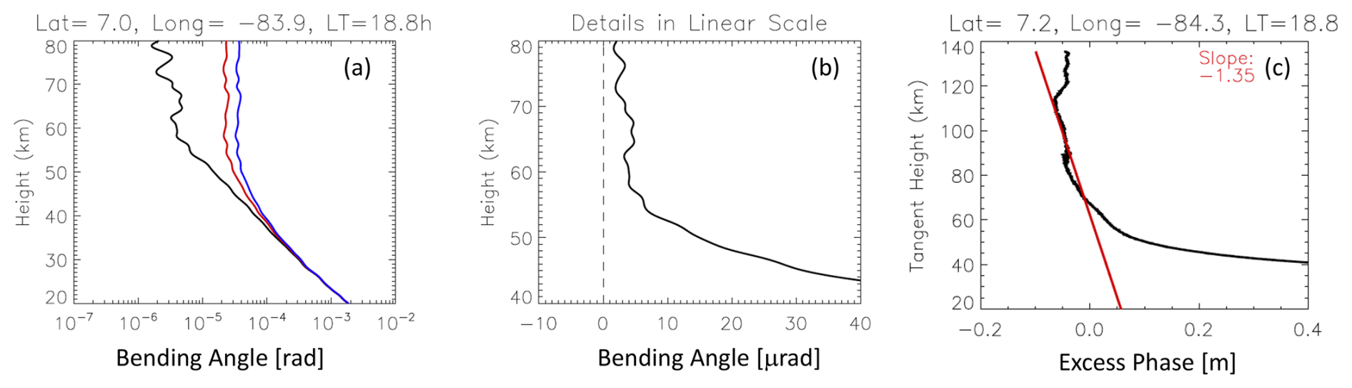
Figure 1 An example of COSMIC-2 atmospheric α profiles in (a) logarithmic and (b) linear scale and (c) the corresponding ϕ_ex profile from 1 January 2022. The red and blue profiles in (a) are the L1 and L2 bending angle α, respectively. The dashed line in (b) indicates no RIE if the α average at 60–80 km is zero. The red line in (c) is a linear fit to the α data between 65 and 120 km, the slope of which is $\mathrm{d}{\mathit{\varphi }}_{\mathrm{ex}}/\mathrm{d}{h}_{\mathrm{t}}$. The units of the bending angle α and excess phase ϕ_ex are indicated in square brackets.

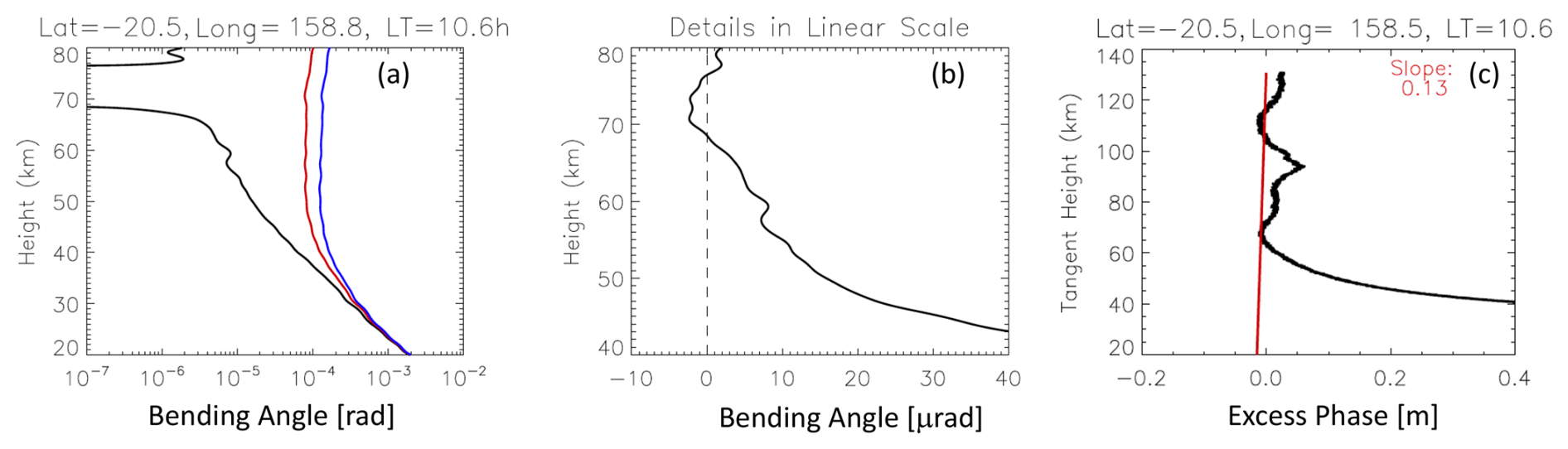
Figure 2 As in Fig. 1 but for another example where an ionospheric E-layer is present in the ϕ_ex profile.

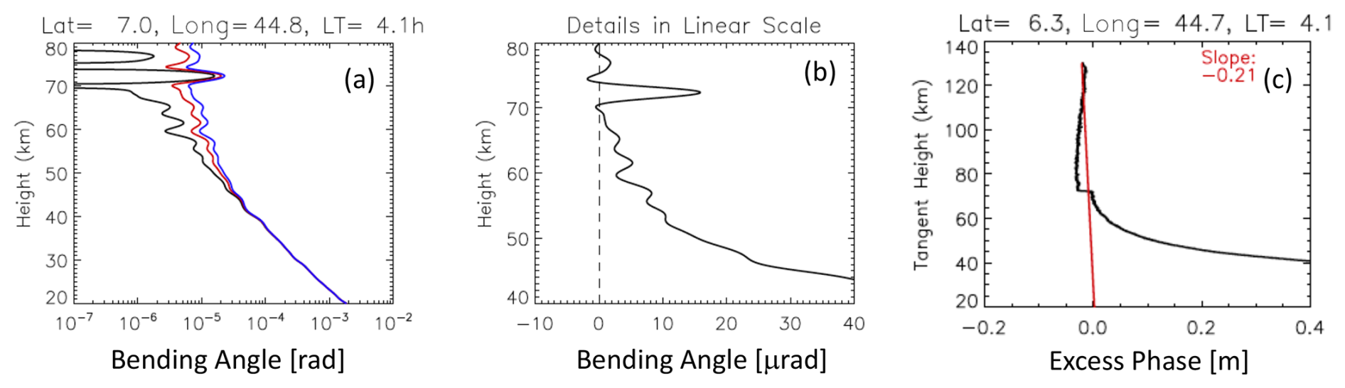
Figure 3 As in Fig. 1 but for a case with a sharp jump in the ϕ_ex profile near 70 km and a moderate derivative $\mathrm{d}{\mathit{\varphi }}_{\mathrm{ex}}/\mathrm{d}{h}_{\mathrm{t}}$.

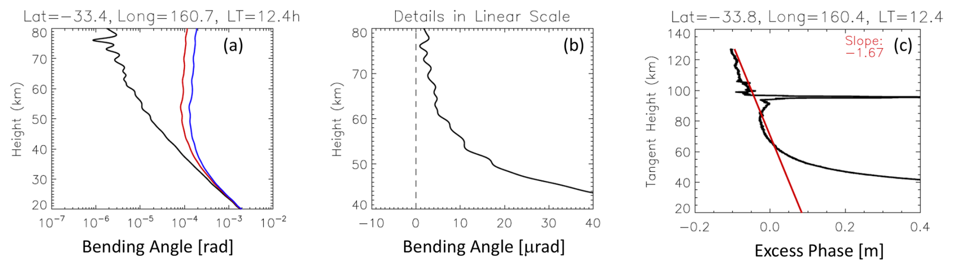
Figure 4 As in Fig. 1 but for a case with a sharp spike in the ϕ_ex profile near 95 km and a significant derivative $\mathrm{d}{\mathit{\varphi }}_{\mathrm{ex}}/\mathrm{d}{h}_{\mathrm{t}}$.

It is important to develop a method that can overcome the noisy or oscillatory nature of α profiles and estimate the RIE that may have an impact on the temperature retrieval in the upper troposphere and stratosphere. A robust RIE algorithm needs to demonstrate the following capabilities: (i) to adequately handle short or sharp spikes in the E-region; (ii) to be self-sufficient in determining the RIE for each individual α profile, regardless of the ionospheric conditions; and (iii) to be able to estimate the RIE in the presence of large noise. Using the relationship between α and $\mathrm{d}{\mathit{\varphi }}_{\mathrm{ex}}/\mathrm{d}{h}_{\mathrm{t}}$ as described by Eq. (6), we introduce an RIE correction scheme for the α profile, which can be implemented at Level-1B ϕ_ex (excess phase) processing. There are several advantages to using the Level-1B data for the RIE correction. They are as follows.

1. ϕ_ex is a more fundamental measurement than α. As discussed above, other processes in the radio wave propagation can induce RIEs even in the situation without bending. Thus, both positive and negative values are physically meaningful and allowed for $\mathrm{d}{\mathit{\varphi }}_{\mathrm{ex}}/\mathrm{d}{h}_{\mathrm{t}}$.

2. The inversion from the ϕ_ex to α profile in RO data reduction can introduce additional noise, which can make the RIE estimation more difficult. The ϕ_ex data do not contain the smoothing parameter and a priori constraints needed in the inversion algorithms. These parameters can affect the RIE determination since they may vary significantly between software developers and versions. In the $\mathrm{d}{\mathit{\varphi }}_{\mathrm{ex}}/\mathrm{d}{h}_{\mathrm{t}}$ method, the least-squared linear fit to the iono-free ϕ_ex profile can use quality control applied directly to the Level-1B data.

3. ϕ_ex contains the information in the L1 (${\mathit{\varphi }}_{{\mathrm{ex}}_{\mathrm{L}\mathrm{1}}}$) and L2 (${\mathit{\varphi }}_{{\mathrm{ex}}_{\mathrm{L}\mathrm{2}}}$) measurements independently, rather than the corrected profile from Eq. (5). The original Level-1B data with the high-rate sampling retain useful insights and allow further investigations on the cause(s) of RIEs.

To estimate the RIE for α, we carry out a linear fit to the iono-free ϕ_ex data at h_t > 65 km for each RO profile independently, i.e.,

$$\begin{array}{}\text{(7)}& {\mathit{\varphi }}_{\mathrm{ex}}=-\mathrm{\Delta }\mathit{\alpha }\cdot h_{\mathrm{t}}+{\mathit{\varphi }}_{\mathrm{0}}{h}_{\mathrm{t}}>\mathrm{65}\mathrm{km},\end{array}$$

where ϕ₀ is the constant from the fitting and the slope $\mathrm{\Delta }\mathit{\alpha }\equiv -\mathrm{d}{\mathit{\varphi }}_{\mathrm{ex}}/\mathrm{d}{h}_{\mathrm{t}}$. Hereafter, we use Δα as an approximation of bending angle α, which is derived from the vertical derivative of excess phase profile. If there is no RIE, Δα=0. Large Δα≠0 values are interpreted as an RIE for the α profile. The 65 km altitude cutoff in the Δα calculation is to ensure that the fitting will not be influenced by the neutral atmospheric bending. To compare with the RIE estimated from the κ method, we simply multiply (Δα₁−Δα₂)² with κ, where Δα₁ and Δα₂ are respectively derived from ${\mathit{\varphi }}_{{\mathrm{ex}}_{\mathrm{L}\mathrm{1}}}$ and ${\mathit{\varphi }}_{{\mathrm{ex}}_{\mathrm{L}\mathrm{2}}}$. As shown and discussed in the following section, there are important differences between the RIE climatologies derived from the κ method and the $\mathrm{d}{\mathit{\varphi }}_{\mathrm{ex}}/\mathrm{d}{h}_{\mathrm{t}}$ method. Note that Eq. (7) does not rely on any auxiliary data or model such as the international reference ionosphere (IRI), nor does it assume the spherical symmetry of the electron density (Ne) profile. As shown in Mannucci et al. (2011) and Coleman and Forte (2017), the spherical symmetry assumption can become problematic for the RIE evaluation in the presence of complex ionospheric structures and small-scale variability of the ionosphere.

Quality control (QC) on the ϕ_ex data is required to ensure the fitting yields a reasonable Δα. Table 1 summaries the QC flags and procedures applied to GNSS-RO data in the RIE estimation. Because of complex impacts from ionospheric variability, the ϕ_ex data processing algorithm needs to deal with large ϕ_ex oscillations properly, especially non-monotonic profiles with multiple extremes at altitudes > 65 km. These extraordinary ϕ_ex profiles include multiple layers with different ϕ_ex slopes in between, large jumps in the measurement, noisy profiles due to ionospheric scintillations, and disturbances from Es layers. With the QC no. 1 and QC no. 2 criteria in Table 1, we ensure that the ϕ_ex profile has enough samples and a good signal-to-noise ratio (SNR) at 60–120 km to yield a useful fit from Eq. (7). Since the GNSS-RO L1 (${\mathit{\varphi }}_{{\mathrm{ex}}_{\mathrm{L}\mathrm{1}}}$) and L2 (${\mathit{\varphi }}_{{\mathrm{ex}}_{\mathrm{L}\mathrm{2}}}$) measurements do not have absolute calibration, they are first initialized using the top value of each RO profile. Hence, the ϕ_ex values at 60–120 km should not be too far from zero (Figs. 1–4). However, profiles with very large ϕ_ex values or large standard deviations about the mean do exist. To deal with these cases, QC no. 3 and OC no. 4 are applied to the ϕ_ex data prior to the fitting. As noted above, Eq. (7) can handle a constant offset in the ϕ_ex data after the data are screened by QC no. 3, but QC no. 4 helps to minimize the impacts from data spikes (e.g., Es) and E-layer residuals (e.g., Fig. 2). Based on our algorithm experiments (see the Discussion section), the ϕ_ex profile is required to have a top reaching a sufficiently high altitude for a reliable RIE estimate to overcome the Es effects that are largely confined to 80–100 km. Lastly, the ϕ_ex data may have a large gap in the profile, which could also yield a problematic fit from Eq. (7) and should be excluded (QC no. 6). In this study we are not interested in very large Δα values that are greater than 2000 µrad (QC no. 7).

Table 1 QC in ϕ_ex data processing for Δα.

Note: *thresholds in QC no. 4 and QC no. 5 require further tests to achieve optical results.

3 RIEs from the ϕ_ex-gradient method

3.1 Δα morphology

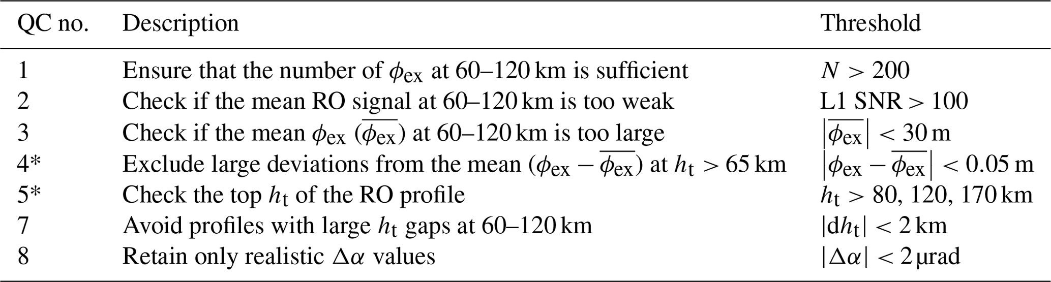
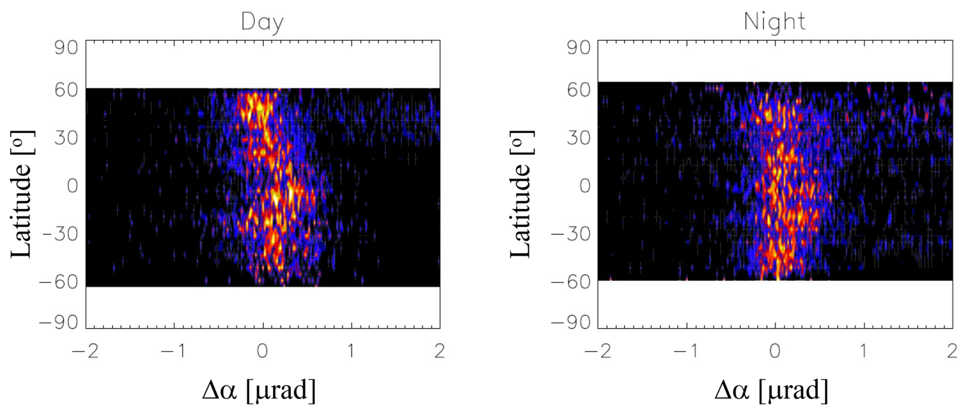
Statistical properties of the Δα estimated from the slope ($\mathrm{d}{\mathit{\varphi }}_{\mathrm{ex}}/\mathrm{d}{h}_{\mathrm{t}}$) at high altitudes vary with local time, latitude, season, and solar activity, and they may also differ from each other depending on the RO receiver type. To examine the probability distribution from different RO receivers, we first derive Δα without imposing QC no. 4 in Table 1 and aggregate the monthly Δα data in terms of a normalized probability density function (PDF) as a function of latitude separately for both day (χ< 90°) and night (χ> 90°). Because of large sampling differences, the PDFs are normalized to the peak value in each latitude bin. Figures 5–8 show the results from COSMIC-1 (January 2013), COSMIC-2 (January 2022), Spire (January 2022), MetOp-B (January 2023), and FY3-E (January 2023). For comparisons under a similar environment, we chose 2013 and 2022–2023 when there were high solar activities. January is a generally higher Ne month in the Southern Hemisphere (SH) due to more solar illumination. The top height of GNSS-RO profiles is required to reach 120 km (QC no. 5) for these comparisons. Not every GNSS-RO sensor has this high-altitude coverage in regular operation (e.g., MetOp and FY3). However, starting in early 2022 MetOp-B and MetOp-C began to acquire GNSS-RO profiles above 120 km routinely. MetOp-B/C satellites have a Sun-synchronous orbit with an Equator crossing time (ECT) of 08:00–10:00 and 20:00–22:00. Thus, the comparison of MetOp-B/C with the COSMIC-1 observations is feasible but from different solar maximum years and with different local time coverage. Both COSMIC-1 and COSMIC-2 constellations, as well as Spire, have a coverage of all local times over a period of 1 month. The new GNSS receivers on FY3-E (March 2022–present) have been providing the RO sampling with a top above 120 km with a varying ECT (04:00–06:00 and 16:00–18:00).

The COSMIC-2 Δα PDFs show a slightly noisy or wider distribution compared to COSMIC-1 (Figs. 5–6). But data from both reveal a larger (more positive) Δα RIE in the SH than in the Northern Hemisphere (NH). This hemispheric difference is more pronounced during the day than at night. The daytime low-latitude PDFs appear to have a longer tail at negative Δα values, which is consistent with the statistics from Spire data (Fig. 7). The Spire Δα PDFs have a width falling between COSMIC-1 and COSMIC-2 but show a similar hemispheric difference. The ϕ_ex measurement noise may contribute partly to the Δα spread, but the RIE is considered to be a major cause of the nonzero Δα and its standard deviation.

The Δα derived from the meteorological satellites (i.e., MetOp-B and FY3-E) (Figs. 8–9), which have a weaker SNR (signal-to-noise ratio) and a higher orbital altitude compared to the COSMIC-1/2 and Spire constellations, tends to have a noisier PDF. It is unclear whether the noisier behavior is related to sampling or orbital parameters or to the RO receiver design and the observing environment on spacecraft. Since MetOp and FY3 employed very different receiver designs but have a similar SNR to Spire, their Δα PDF difference from COSMIC and Spire might be related to the orbital altitude. Another factor is the receiver environment on the spacecraft. The RO receivers on COSMIC and Spire satellites are considered to be the primary payload and do not have much interference from other instruments on board. Interference and multipath issues can be a susceptibility problem when multiple instruments are on board spacecraft like MetOp and FY3. Interferences from other radio frequencies and structures may affect the RO receiver performance for high-quality ionospheric measurements.

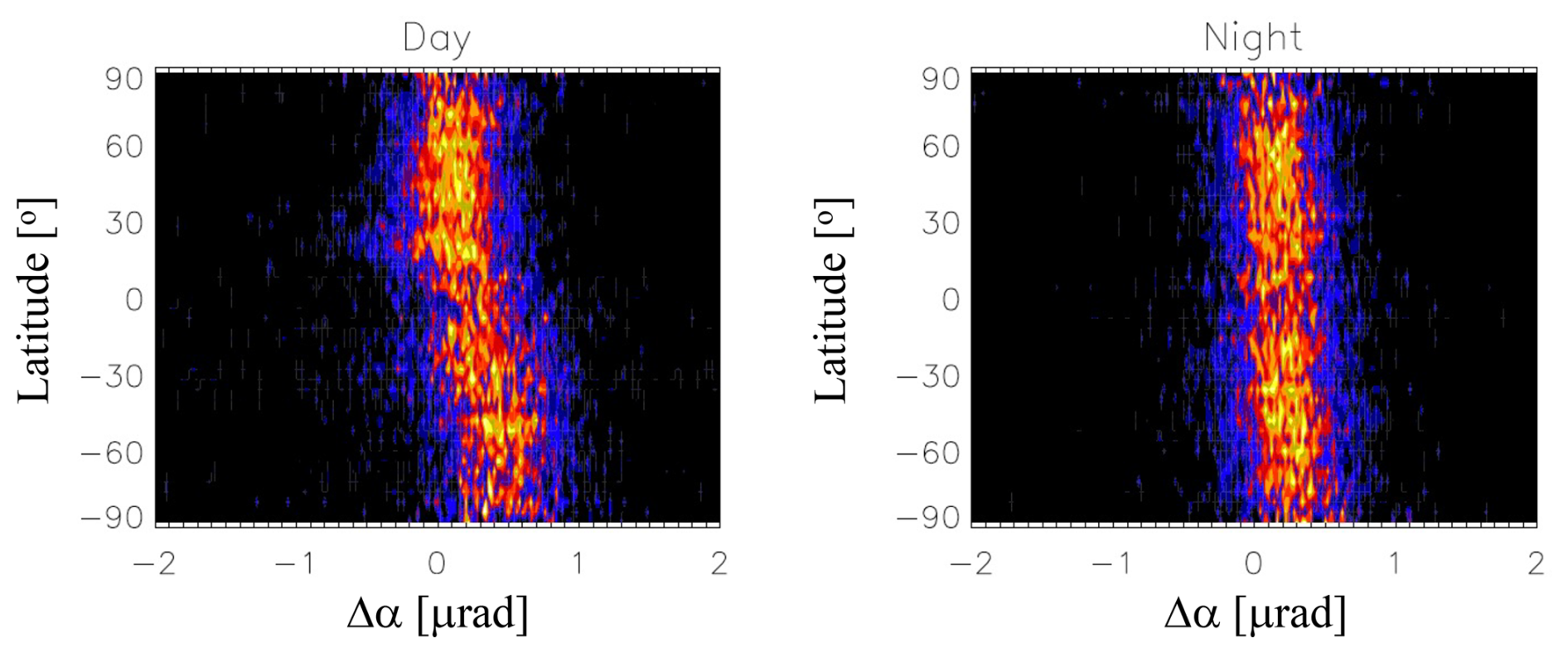
Figure 5 Latitude dependence of the probability density function (PDF) of COMSIC-1 Δα in µrad for day and night from January 2013. The PDF is normalized independently to its peak value at each 4° latitude bin. The PDF colors vary linearly between 0 (black) and 1 (yellow).

Figure 6 As in Fig. 5 for COMSIC-2 from January 2022.

Figure 7 As in Fig. 5 for Spire from January 2022.

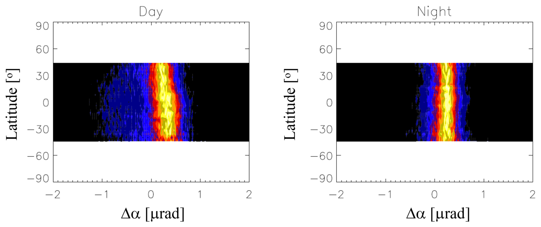
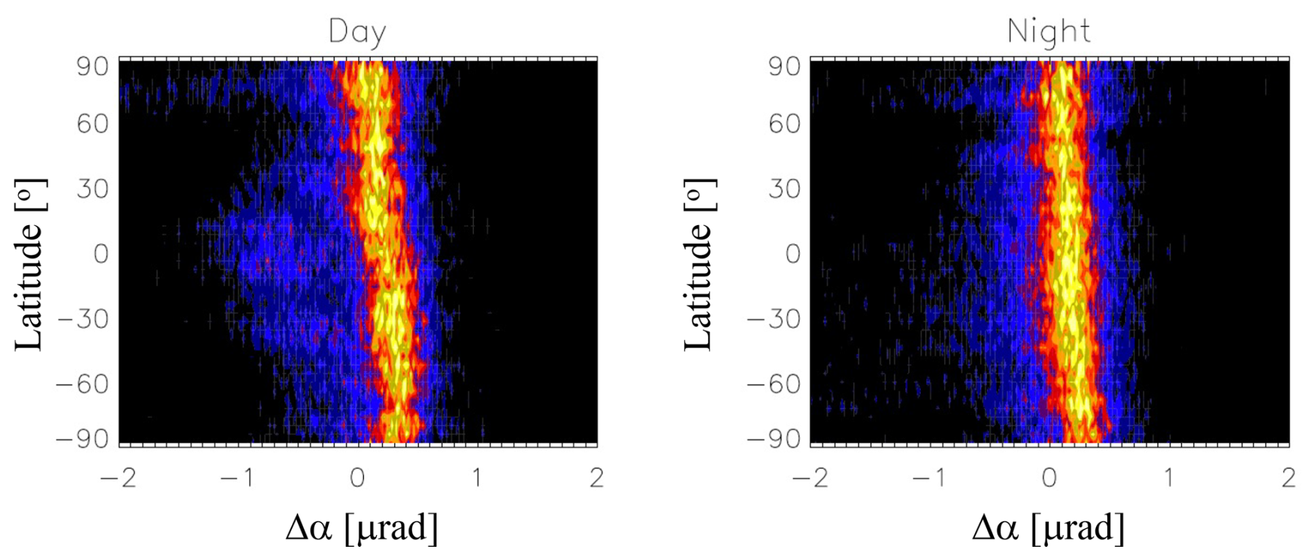
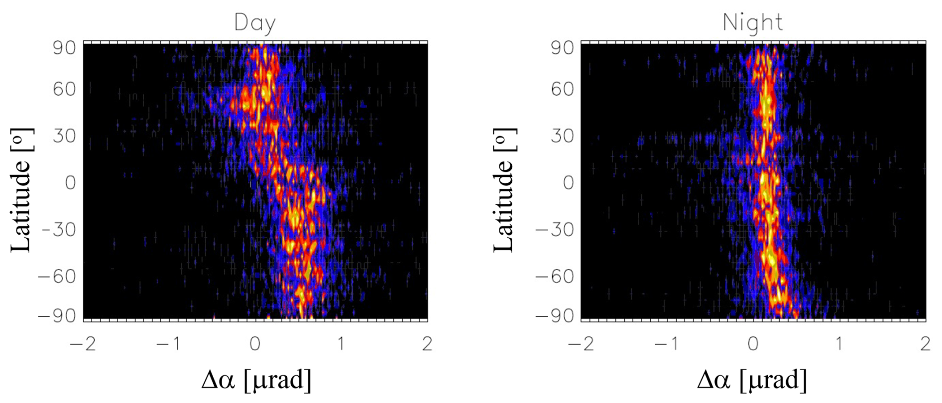
Figure 8 As in Fig. 5 for MetOp-B from January 2023. MetOp-C (not shown here) has very similar Δα PDFs to MetOp-B.

Figure 9 As in Fig. 5 for FY3-E from January 2023.

3.2 Diurnal and solar cycle variations

The mean (μ) and standard deviation (σ) of Δα from January and July 2013 show a nonuniform distribution that varies with local solar time (LST), geographical location, season, and solar activity (Figs. 10–11). To illustrate the LST and latitudinal dependence, we used the COSMIC-1 measurements from January and July 2013 when solar activity was near its maximum. The monthly data are aggregated to 4° latitude and 2 h LST bins using the quality screening criteria as shown in Table 1 with QC no. 4 and QC no. 5 (120 km). For the solar cycle variation, we used all COSMIC-1 data from 2006 to 2019 and averaged all LSTs to produce a time series of monthly zonal mean. During most of its mission (2007–2017), COSMIC-1 had a full diurnal sampling from its six-satellite constellation on a precessing orbit. But in the later period, failure of some satellites degraded the diurnal sampling and yield a slightly noisy result in the time series.

There are significant differences between the Δα morphologies derived from the $\mathrm{d}{\mathit{\varphi }}_{\mathrm{ex}}/\mathrm{d}{h}_{\mathrm{t}}$ method (Figs. 10–11) and the κ method (Fig. 12). The $\mathrm{d}{\mathit{\varphi }}_{\mathrm{ex}}/\mathrm{d}{h}_{\mathrm{t}}$ method reveals both negative and positive values in the Δα distributions, showing mostly negative values during the daytime and positive at night. The κ method always produces a negative RIE value from the product of a negative κ value and (Δα₁−Δα₂)², regardless of day and night. To further illustrate their differences, we applied the same method (Eq. 7) separately to the ϕ_exL1 and ϕ_exL2 data and derived $\mathrm{\Delta }{\mathit{\alpha }}_{\mathrm{1}}\equiv -\mathrm{d}{\mathit{\varphi }}_{\mathrm{exL}\mathrm{1}}/\mathrm{d}{h}_{\mathrm{t}}$ and $\mathrm{\Delta }{\mathit{\alpha }}_{\mathrm{2}}\equiv -\mathrm{d}{\mathit{\varphi }}_{\mathrm{exL}\mathrm{2}}/\mathrm{d}{h}_{\mathrm{t}}$. Unlike the (Δα₁−Δα₂)² distribution derived using an ionospheric electron density model (Angling et al., 2018), the (Δα₁−Δα₂)² distributions and variations derived from the multiyear COSMIC-1 RO data (Fig. 12) are more realistic, and they can be properly compared to the Δα morphology derived from the $\mathrm{d}{\mathit{\varphi }}_{\mathrm{exL}\mathrm{2}}/\mathrm{d}{h}_{\mathrm{t}}$ method.

Since the (Δα₁−Δα₂)² distribution was introduced to provide a leading-order (f⁻²) correction of the ionospheric impact on the radio wave propagation, it is expected that the higher-order and bending-independent RIEs may be not captured by the κ method. In other words, the distribution and variation of (Δα₁−Δα₂) difference cannot be fully characterized by (Δα₁−Δα₂)² . For the evaluation of RIE impacts on temperature and humidity in the later section, (Δα₁−Δα₂) represents the persistent bias term in the inversion problem applied to the α data. As seen in Fig. 10, not only are the two subtropical Δα peaks negative during the daytime, but they also exhibit different mean values with a larger magnitude in the NH. This subtropical difference is much less pronounced in the (Δα₁−Δα₂)² distribution (Fig. 12). In addition, the summer–winter contrast (January vs. July) is more pronounced in the Δα distribution than in the (Δα₁−Δα₂)² as used by the κ method. The seasonal and hemispheric differences between the Δα and (Δα₁−Δα₂)² morphologies are reflected in their solar cycle variations as well. The κ-method correction with (Δα₁−Δα₂)² shows a variation symmetric about the Equator (Danzer et al., 2020), similar to the distribution revealed in Fig. 12c. Thus, depending on how the RIE is derived, the application of two different RIE corrections as described above would likely have different impacts on the neutral atmospheric retrievals and the α data assimilation.

Solar cycle variations are more pronounced in the daytime Δα than in the nighttime (Fig. 11), as expected for the RIE associated with the photoionization in the ionosphere. The Δα time series derived from the $\mathrm{d}{\mathit{\varphi }}_{\mathrm{ex}}/\mathrm{d}{h}_{\mathrm{t}}$ method shows a larger negative daytime RIE with a hemispheric asymmetry during the solar maximum years, but a larger positive nighttime RIE during the solar minimum years. At high latitudes, a summertime positive RIE appears to be a repeatable phenomenon with slightly higher values in the NH nighttime. There is an indication of weak solar cycle variations in the daytime high-latitude Δα. The solar cycle variations from COSMIC-1 are consistent with the MetOp-A/B/C observations (not shown), which have global coverage at two fixed LSTs. In summary, the solar cycle variation of the RIE derived from the $\mathrm{d}{\mathit{\varphi }}_{\mathrm{ex}}/\mathrm{d}{h}_{\mathrm{t}}$ method differs substantially from those from the κ method based on (Δα₁−Δα₂)². The time series of RIEs derived from the κ method exhibits little high-latitude variation and has a similar daytime solar cycle in both NH and SH subtropics.

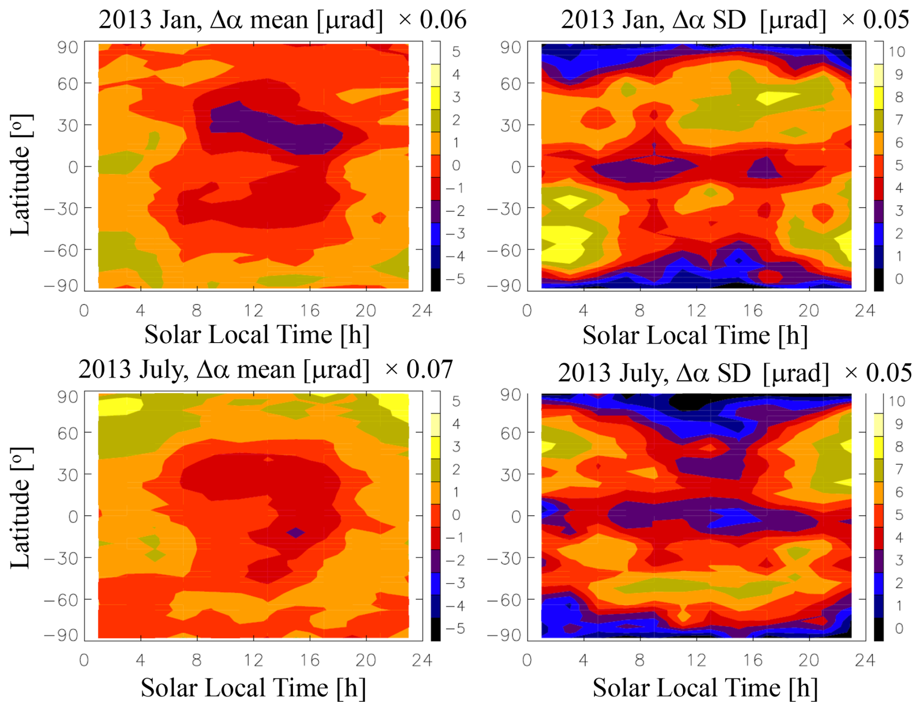
Figure 10 Latitude (4° bin) and solar local time (2 h bin) dependence of COSMIC-1 RIE Δα mean (μ) and standard deviation (σ) from January and July 2013. All color numbers have a scale factor indicated at the top of each color bar.

In addition to the mean distribution of Δα, its spatiotemporal variability also plays an important role in the RIE correction. If the underlying processes are not random and vary nonlinearly with RIE, a spatial or temporal average may not eliminate the RIE impacts on the neutral atmosphere retrievals. Because the fast and nonlinear ionospheric processes may impact the RIE, we further characterize the Δα variation in terms of mean (μ) and standard deviation (σ) on a monthly gridded map. In this calculation we compute the monthly μ and σ maps of Δα on a latitude × longitude (4° × 8°) grid for every 2 h LST bin. Figure 10 shows the LST and latitude distributions of μ and σ from January and July 2013. Both variables exhibit a strong diurnal variation, which is latitude-dependent, with a large σ amplitude at midlatitudes and during the nighttime. The correlations between the μ and σ distributions are complicated, but in both months the σ amplitude can be greater than the Δα mean, particularly in the nighttime. The seasonal dependence of the σ diurnal variation shows a larger amplitude at midlatitudes in the winter daytime and evening and in the summer nighttime.

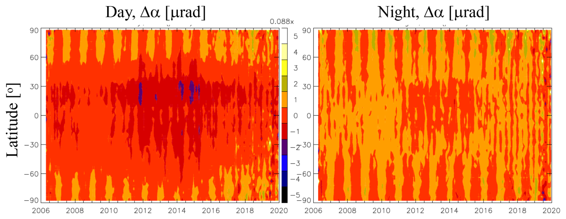
Figure 11 Long-term variations of the daytime and nighttime mean Δα from COSMIC-1 as a function of latitude during 2006–2020. All color numbers have a scale factor indicated at the top of each color bar.

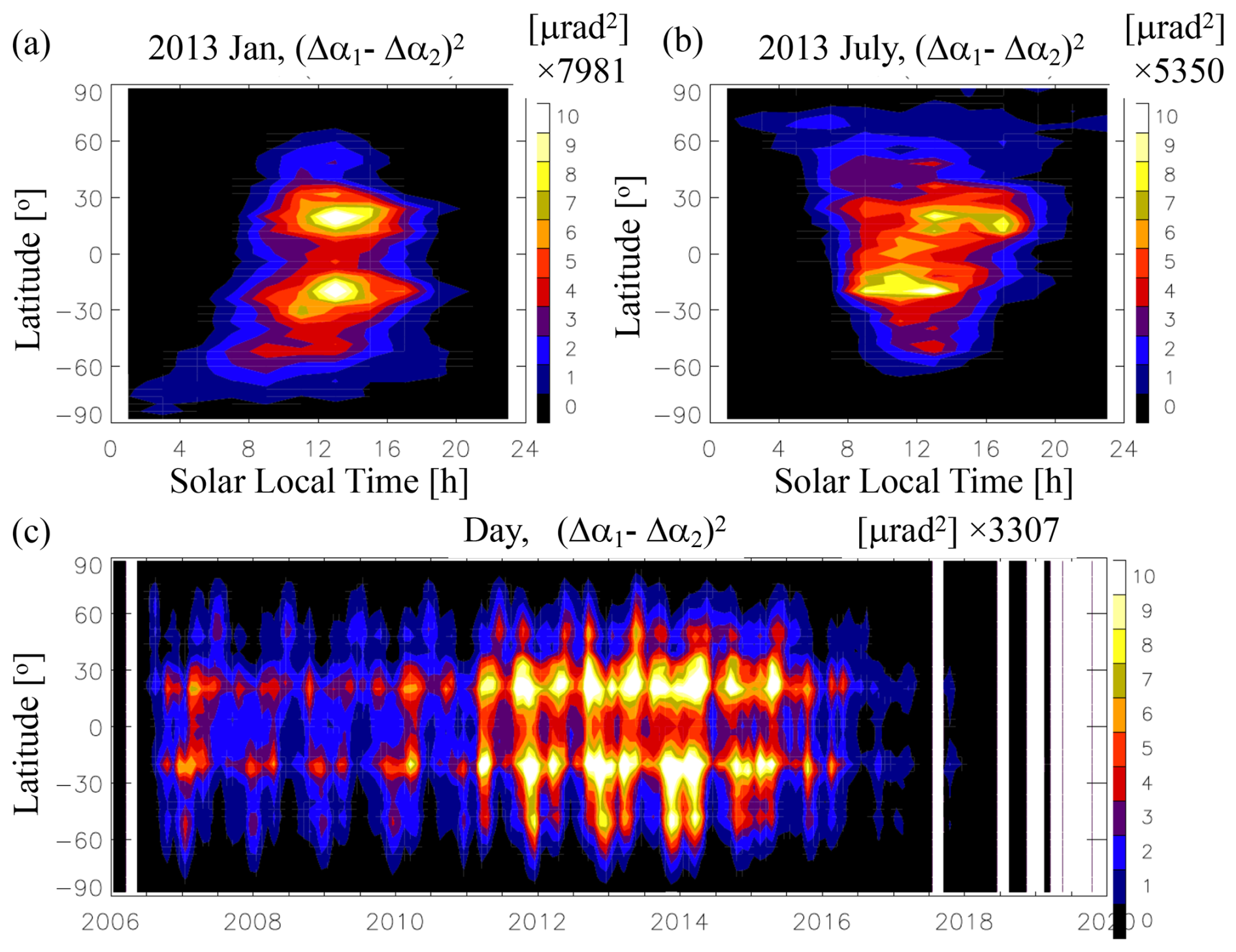
Figure 12 The (Δα₁−Δα₂)² distribution and variations derived from the COSMIC-1 data using $\mathrm{\Delta }{\mathit{\alpha }}_{\mathrm{1}}\equiv -\mathrm{d}{\mathit{\varphi }}_{\mathrm{exL}\mathrm{1}}/\mathrm{d}{h}_{\mathrm{t}}$ and $\mathrm{\Delta }{\mathit{\alpha }}_{\mathrm{2}}\equiv -\mathrm{d}{\mathit{\varphi }}_{\mathrm{exL}\mathrm{2}}/\mathrm{d}{h}_{\mathrm{t}}$. The (Δα₁−Δα₂)² distribution here can be compared to the RIE derived from the κ method in Fig. 10 by multiplying a κ value between −10 and −15 rad⁻¹ for 60 km. All color numbers have a scale factor indicated at the top of each color bar.

3.3 Longitudinal variations and dependence on geomagnetic field

It is well recognized in previous studies that ionospheric variability can be also driven by the atmospheric waves originating in the lower atmosphere and the geomagnetic forcing from above (Forbes et al., 2006; Immel et al., 2006). The underlying ionospheric processes of RIEs are likely dependent on geomagnetic activity as well as on longitudinal and seasonal wave variability. Thus, it is important to quantify the Δα distribution and its variations in the geographical and geomagnetic coordinate systems. The monthly averaged geographical Δα maps derived from COSMIC-1 data for January and July 2013 show a large nighttime longitudinal variation in Δα (Fig. 13), which may be induced by the atmospheric planetary waves forced in the lower atmosphere and mesosphere. There is also an indication that the daytime Δα distributions vary slightly with the geomagnetic field at low and middle latitudes in both seasons. At high latitudes, however, there is no noticeable Δα variation or connection to the auroral activity in the polar caps. The dependence of RIE on the geomagnetic field variation is expected from the high-order ionospheric effect (Hoque and Jakowski, 2007), and such RIEs can be both positive and negative (Vergados and Pagiatakis, 2011).

It is interesting to note that the nighttime Δα distributions bear a strong resemblance to those derived for the Es climatology in summer and winter (Wu et al., 2005; Arras et al., 2009). Previous studies showed that the occurrence of Es from global GNSS-RO observations tends to peak at 90–110 km altitudes near midlatitudes during the summer months and is strongly modulated by the solar diurnal and semidiurnal migrating tides. Syndergaard (2000) discussed the Es-induced morphology of RIE, showing a frequent influence of Es below the occurrence altitude. This study also suggested the RIE correction scheme for the Es-induced errors.

However, it remains unclear to what extent Es may contribute to the RIE amplitude and variability. Although the $\mathrm{d}{\mathit{\varphi }}_{\mathrm{ex}}/\mathrm{d}{h}_{\mathrm{t}}$ method attempts to minimize the Es impacts using more measurements from higher altitudes (Fig. 2), the RIE maps from Fig. 13 seem to indicate that Es may have a significant role in the nighttime RIE variation. The fact that $\mathrm{d}{\mathit{\varphi }}_{\mathrm{ex}}/\mathrm{d}{h}_{\mathrm{t}}$ is correlated more with Es than with the geomagnetic field suggests that the spatial inhomogeneity effect might play a significant role in RIE. As described by Syndergaard and Kirchengast (2022) in a bi-local ray-trace model, an RIE would arise due the L1 and L2 path split at the tangent point (Appendix A). Most of the contribution to RIE comes from the near-side propagation after the split, where the L1 and L2 phase advance (in plasma propagation) and phase delay (from F-region bending) can go through significantly different paths. Because the E- and F-region ionospheric variabilities are driven by different processes, their contributions to the RIE may depend on latitude, longitude, local time, and geomagnetic field. As elucidated by Syndergaard and Kirchengast (2022), path differences between the L1 and L2 propagation in a 3D structured ionosphere are the major cause of various RIEs, which can vary with the geomagnetic field and the spatial distribution and gradient of electron density. However, in a comparison between the simulated bi-local and κ-model RIEs, Liu et al. (2024) found a significant geomagnetic impact through high-order contributions to the refractive index but no significant effect from ionospheric asymmetry. One possibility of the negligible impact from ionospheric asymmetry in the ray-trace simulations by Liu et al. (2024) is the way the asymmetry was incorporated into the model. In the study by Liu et al. (2024), an asymmetry factor was induced to partition the vertical TEC (vTEC) on the near- and far-side ionosphere divided at the tangent point. This is likely a different inhomogeneity from the propagation path split implied by Syndergaard and Kirchengast (2022). It would require a strong vertical gradient in Ne such as Es to split the propagation paths between L1 and L2. The vTEC partitioning approach implemented by Liu et al. (2024) may not induce an extraordinarily strong vertical Ne gradient in the inhomogeneous ionosphere to test the impacts from the case with fine structures. Hence, depending on the relative importance of these contributions, the RIE correction methods are likely to yield different impacts on the neutral atmospheric measurements.

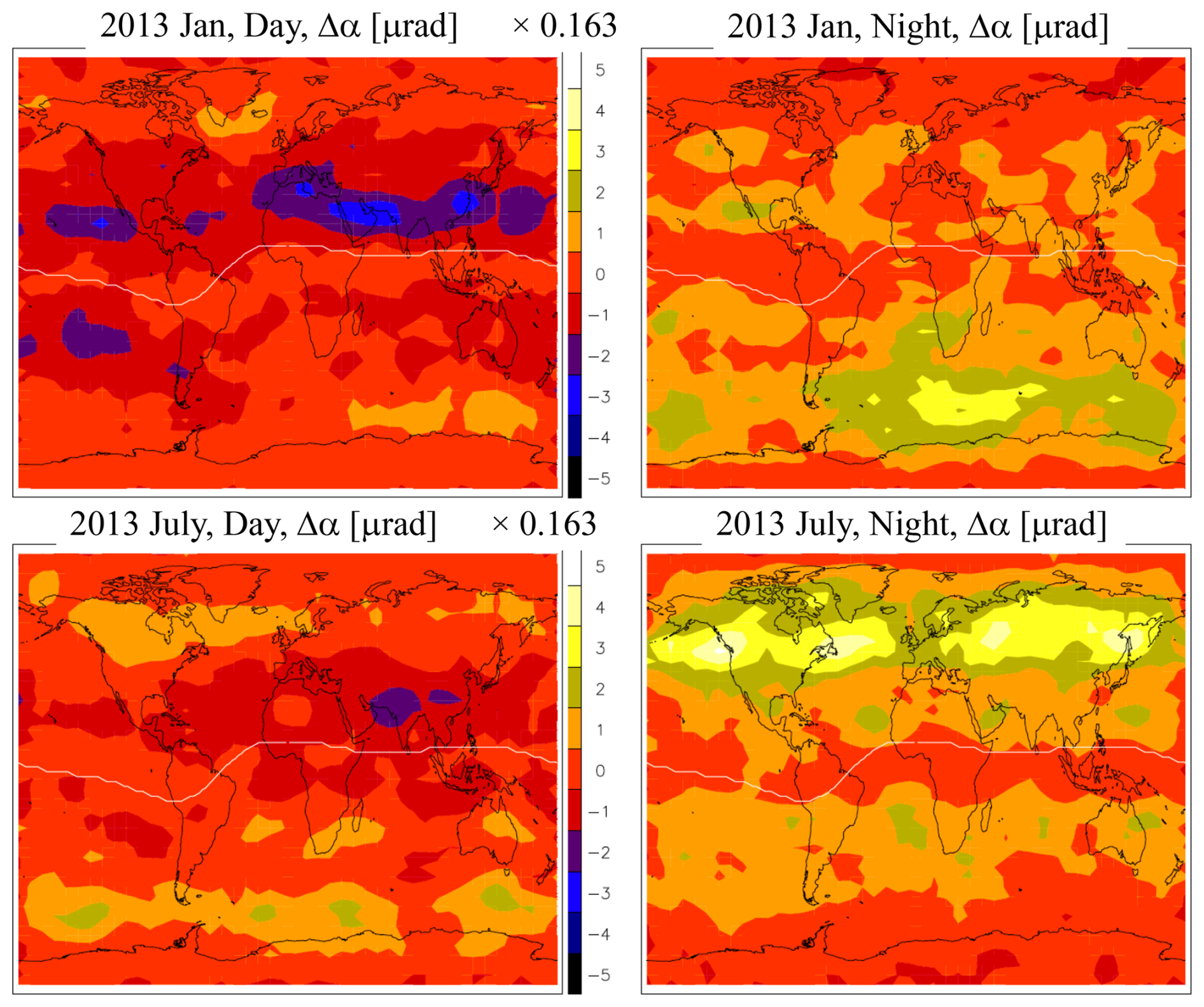
Figure 13 Geographical maps of the Δα derived from COSMIC-1 $-\mathrm{d}{\mathit{\varphi }}_{\mathrm{exL}\mathrm{1}}/\mathrm{d}{h}_{\mathrm{t}}$ measurements for January and July 2013; the white lines display positions of the geomagnetic Equator. All color numbers have a scale factor indicated at the top of each color bar.

4 RIE impacts on data assimilation (DA)

4.1 Goddard Earth Observing System for Instrument Teams (GEOS-IT)

To quantify potential impacts of the observed Δα morphology on the neutral atmosphere, we conducted several data assimilation (DA) experiments using the GEOS-IT DA configuration of the NASA GMAO/GSFC (https://gmao.gsfc.nasa.gov/GMAO_products/GEOS-IT, last access: 8 February 2025). GEOS-IT retains many characteristics of the GEOS Forward Processing System, including the spatial resolution (∼ 50 km) and the use of a three-dimensional variational (3D-Var) DA algorithm, and allows the instrument teams to benefit from many model enhancements of GEOS, leading to more realistic representations of moisture, temperature, land surface, and analysis changes that introduce the most modern new satellite observations into the system. The GEOS-IT configuration employed in this study (GEOS-5.27 DA system) assimilates GNSS-RO α observations with a 6 h update cycle (McCarty et al., 2016; Gelaro et al., 2017) using the RO forward operator as in the operational NCEP (National Centers for Environmental Prediction) bending angle method (NBAM) (Cucurull et al., 2013). As shown in Cucurull et al. (2014), the GNSS-RO observations have both direct and indirect impacts on the quality and skills of analyses and forecasts of NWP systems. The RO assimilation results in a more accurate bias correction for infrared and microwave radiance measurements and therefore leads to more effective use of satellite radiances by allowing more radiance data that satisfy the quality control requirement. This indirect impact has made the GNSS-RO observations more valuable, even if the number of profiles is relatively small compared to the radiance measurements. Because the GNSS-RO technique is essentially traced to the SI length unit, with little dependence on radiometric calibration, it serves as an anchor of the radiance bias correction for the microwave and IR sounders.

The direct impact of RO data comes from their α sensitivity to the temperature in the upper troposphere and stratosphere. The RO measurements help to constrain the temperatures at 8–40 km in all weather conditions with global and full local time coverage. As a measurement forward model, the ROPP package produces the α data and their errors from the ϕ_ex data (Healy et al., 2007; Cucurull et al., 2013, 2014; Zhang et al., 2022). The GEOS DA algorithm for the RO observations assumes the zero α bias without RIE. As remarked on in previous DA studies above ∼ 30–40 km (Healy et al., 2007), the RIE correction schemes for the α data analysis are important and can affect the DA data quality if not implemented, such as systematic α errors associated with the persistent influence of the ionospheric processes. Despite the effort to minimize the RIE impact by increasing RO measurement uncertainty at altitudes above 40 km, RIE impacts are still evident in the resulting analysis data (Danzer et al., 2013).

The RO observation data used in the DA impact study contain data mostly from COSMIC-1 with a global distribution. The observation error used in the GEOS-IT DA is mostly identical to the NCEP system where the final observation errors are inflated at the super-obbing stage. Super-obbing is a technique to reduce redundant information in the observational data and the data density (Purser et al., 2000). The observation error plays a key role in determining the weight between the model forecast and RO observations in the DA, which is a function of latitude and height. In the next section we introduce the ϕ_ex-based RIE correction scheme as described in Sect. 3 and carry out a set of DA experiments to quantify the impact of RO data with and without the RIE on the GEOS-IT DA products.

4.2 DA experiments

To assess the RIE impacts on DA products, we performed GEOS-IT experiments for Dec–Jan of 2016/2017 using the values derived from the $\mathrm{d}{\mathit{\varphi }}_{\mathrm{ex}}/\mathrm{d}{h}_{\mathrm{t}}$ method (Sect. 2.2). In this experiment period, about 2000 α profiles were analyzed per day from multiple GNSS-RO missions (i.e., GRACE, MetOp-A, and COSMIC-1). The horizontal resolution of GEOS-IT analyses and forecasts is ∼ 50 km, and results were archived at 72 model layers from the surface to ∼ 1 Pa (∼ 80 km). Four DA experiments were conducted: (1) a control (CTL) experiment that assimilates all RO observations assuming no RIE bias, (2) a GPS-denial (NoGPS) experiment excluding all RO data, (3) a constant bias (BiasM2) experiment adding a large constant RIE ($\mathrm{\Delta }\mathit{\alpha }=-\mathrm{2}$ µrad) to all RO data, and (4) the $\mathrm{d}{\mathit{\varphi }}_{\mathrm{ex}}/\mathrm{d}{h}_{\mathrm{t}}$-derived bias experiment (BiasLST) incorporating the latitude- and LST-dependent RIE in α that is similar to the COSMIC-1 observation as shown in Fig. 14.

The month of December 2016 was used to spin up the GEOS-IT analysis forecast system, and the RO data were injected starting from 1 January 2017 for the RIE impact experiments. The objective of these experiments is to quantify the potential impacts of the RIE bias from assimilating the α data with the recent upgrades of the GEOS-IT system (model and DA algorithms). We compared the 1–10 January GEOS-IT analyses by differencing each experiment from CTL for the zonal mean temperatures as well as for hourly means in the middle and upper atmosphere. The importance of RIE impacts depends on the RIE amplitude relative to atmospheric variability at each altitude and how much the GNSS-RO measurements are weighted in the DA system. The GEOS-IT α measurement error covariance matrix used in all DA experiments is identical to the normal RO data assimilation. The α error covariance matrix was designed to reduce the weighting on the RO α data at higher altitudes so that their errors there do not impact the lower atmosphere significantly. Nevertheless, the DA results from the α data with an RIE can still have non-negligible impacts on the DA data in the middle atmosphere.

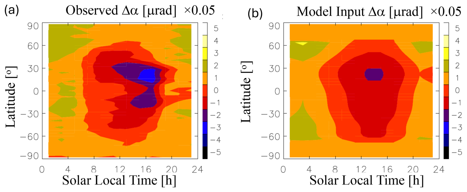
Figure 14 (a) Annual mean Δα variations derived from 2013 COSMIC-1 data. (b) Parameterized Δα variations used as the RIE input for the “BiasLST” DA experiment. All color numbers have a scale factor indicated at the top of each color bar.

4.3 RIE impacts on temperature

The RIE impacts on the DA results tend to grow with time and height in amplitude, despite the reduced sensitivity to the RO α measurement in the upper atmosphere. We chose the 5–7 d period after the GPS measurements are injected with a bias or denial to characterize an accumulated impact from the spatiotemporal growth of the DA system. During the initial growth period (0–5 d), the DA system continues to inject the biased or denied RO data and the rate of growth between CTR and other perturbed runs appears to be large. The growth rate of differences slows down on days 5–7, which yields a better characterization of the RIE impacts.

The 3 d (5–7 January) averaged temperature differences between the CTL and the perturbed experiments (NoGPS, BiasM2, and BiasLST) show significant GPS and RIE impacts on the GEOS-IT analyses (Figs. 15–17). The zonal mean differences (Fig. 15) display the most prominent impacts at high latitudes in the upper stratosphere (above ∼ 30 km). Compared to the NoGPS impacts (Fig. 15a), the GNSS-RO data with an unrealistically large (2 µrad) bias (Fig. 15b) appear to do more harm than good for the DA, showing a bias of 3–30 K in the upper atmosphere and 0.3–0.6 K in the troposphere. The large biases in the upper atmosphere suggest that the DA system trusts the GNSS-RO measurements, with an accuracy better than 2 µrad at these altitudes. In the BiasLST case where the RIE input uses a more realistic value (∼ 0.05 µrad) during the daytime, the RIE impact is reduced to ∼ 1–3 K in the upper stratosphere. The magnitudes of temperature error introduced by this RIE specification (Fig. 14) are comparable to the results reported by Danzer et al. (2020) from the κ method.

In the lower troposphere the GNSS-RO contribution to the DA comes primarily from an indirect impact in which the RO data help to correct the radiance bias between microwave and infrared sounders and allow more radiance data to be assimilated (Healy et al., 2005; Cucurull et al., 2014). The CTL–NoGPS differences (Fig. 15b) show that the impacts of GNSS-RO data are mostly in the polar regions with a temperature improvement of ∼ 0.3–0.9 K. These impacts extend to the lowermost of the polar atmosphere. The large RIE bias (BiasM2, Fig. 15d) has a comparable (0.3–0.6 K) impact on the lower polar atmosphere. For the realistic RIE bias (BiasLST), the impacts are mostly small (< 0.3 K) in the lower troposphere.

It is interesting to observe that the GNSS-RO impacts largely reside in the high-latitude polar regions, which appears to be the case for the denial (NoGPS) and perturbed experiments. These results are consistent with some of the earlier studies with RO-denial experiments, showing a larger impact at higher latitudes (Bonavita, 2014; Cucurull and Anthes, 2015). It is worth pointing out that the large impacts in the polar region occur from day 1 (not shown) when the RO data are injected and exhibit similar magnitude throughout the entire January experiment period. Although the sign of RIE-induced biases may change with time, as seen in planetary wave progression, the largest RIE amplitudes always reside at high latitudes. Because direct and indirect impacts from the GNSS-RO observations may act collectively in the DA output (Healy et al., 2005), these DA experiments seem to indicate that in the RIE impacts might be larger in the region where wave activity is stronger.

In the upper atmosphere where the solar migrating tides become dynamically dominant, the impact of diurnally varying RIEs on these processes needs to be quantified globally. As detailed in Appendix B, the local-time-dependent RIE (BiasLST), despite inducing a mean temperature bias in the mesosphere, does not produce significantly large impacts on the tidal amplitudes there since these waves are locked in phase with the solar forcings from the troposphere and stratosphere.

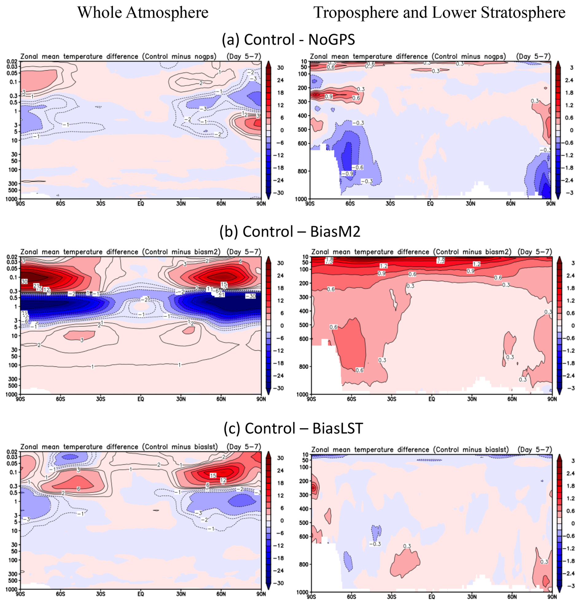
Figure 15 The zonal mean temperature differences between controlled and perturbed experiments. A different color scale is used for the lower atmosphere to highlight small values in this region.

5 Discussion

5.1 Negative and positive RIE values

Causes of RIE are complex because of higher-order effects on the refractive index and effects of the propagation path difference between two frequency bands. Collectively, these effects can induce an RIE from the dual-frequency method if the radio wave propagation through a structured and anisotropic ionosphere (e.g., Davies, 1965; Kindervatter and Teixeira, 2022). Brunner and Gu (1991) modeled the higher-order terms from the series expansion of the refractive index, including the second-order effect from the path difference between the L1 and L2 frequencies and the third-order effect from the geomagnetic field. While the second-order RIEs are mostly negative, the third-order RIEs can be both positive and negative. To quantify the RIE for ground-based receivers, Hoque and Jakowski (2007) developed a correction algorithm that can be applied to real-time GNSS applications and reduce the higher-order phase errors.

In GNSS-RO applications, studies have also found that the second-order RIEs are mostly negative (Liu et al., 2013) and the third-order could have both positive and negative values in α and refractive bias depending on the viewing geometry with respect to the geomagnetic field (Vergados and Pagiatakis, 2011; Qu et al., 2015; Li et al., 2020). These model simulations all suggested a relatively small RIE value that is typically less than 0.1 µrad, generally smaller than what was observed with the $\mathrm{d}{\mathit{\varphi }}_{\mathrm{ex}}/\mathrm{d}{h}_{\mathrm{t}}$ method introduced in Sects. 2 and 3. Nevertheless, the positive and negative Δα values seen in Figs. 5–9 suggest that the first- and second-order RIE effects are equally important. Examining the mean deviation between CHAMP and COSMIC-1 α and a climatology model at 60–80 km altitudes, Li et al. (2020) also reported positive and negative values of RIE, showing larger negative RIEs in the daytime and relatively smaller positive RIEs at night, as seen in Fig. 10. Note that this study did not use any climatology model for α, and the $\mathrm{d}{\mathit{\varphi }}_{\mathrm{ex}}/\mathrm{d}{h}_{\mathrm{t}}$ method is self-sufficient with an empirical linear fitting to each individual profile. In summary, compared to the idealized model simulations, the large variability in the observed positive and negative Δα reflects the complex nature of RIEs in the dynamical ionosphere.

5.2 Impacts of Es and RO top height

An Es layer can produce large RIEs near the layer heights with a long tail extending to lower tangent heights in the GNSS-RO profile (Syndergaard, 2000; Syndergaard and Kirchengast 2022). If the RO measurements stop at or below the Es layer, the $\mathrm{d}{\mathit{\varphi }}_{\mathrm{ex}}/\mathrm{d}{h}_{\mathrm{t}}$ method can be significantly affected by the Es tail and lead to an overestimated RIE. In some GNSS-RO operations (e.g., MetOp), the top of RO data acquisition is often capped at ∼ 85 km. To quantify effects from this low RO top height, we took advantage of the experimental MetOp-A data on 2020D161–2020D254 (9 June–10 September 2020) when the high-rate (100 Hz) GNSS-RO acquisition reached up to ∼ 290 km. This dataset allows us to quantify the RO top impact from different truncation heights.

In this comparative analysis, the $\mathrm{d}{\mathit{\varphi }}_{\mathrm{ex}}/\mathrm{d}{h}_{\mathrm{t}}$ method was applied to the same experimental MetOp-A data from 9 June–10 September 2020 but from different RO truncation tops: 90, 120, and 170 km. The 90 km truncation represents some missions before 2020 such as MetOp and SACC when the high-rate RO data acquisition stopped at ∼ 85 km. The 120 km truncation height has been adopted by several missions (e.g., COSMIC-1, TSX, FY3), whereas the 170 km top operation corresponds to some of the recent commercial GNSS-RO constellations (e.g., Spire and PlanetiQ). More detailed information on the RO sampling parameters of the past and current GNSS-RO missions can be found in Appendix A.

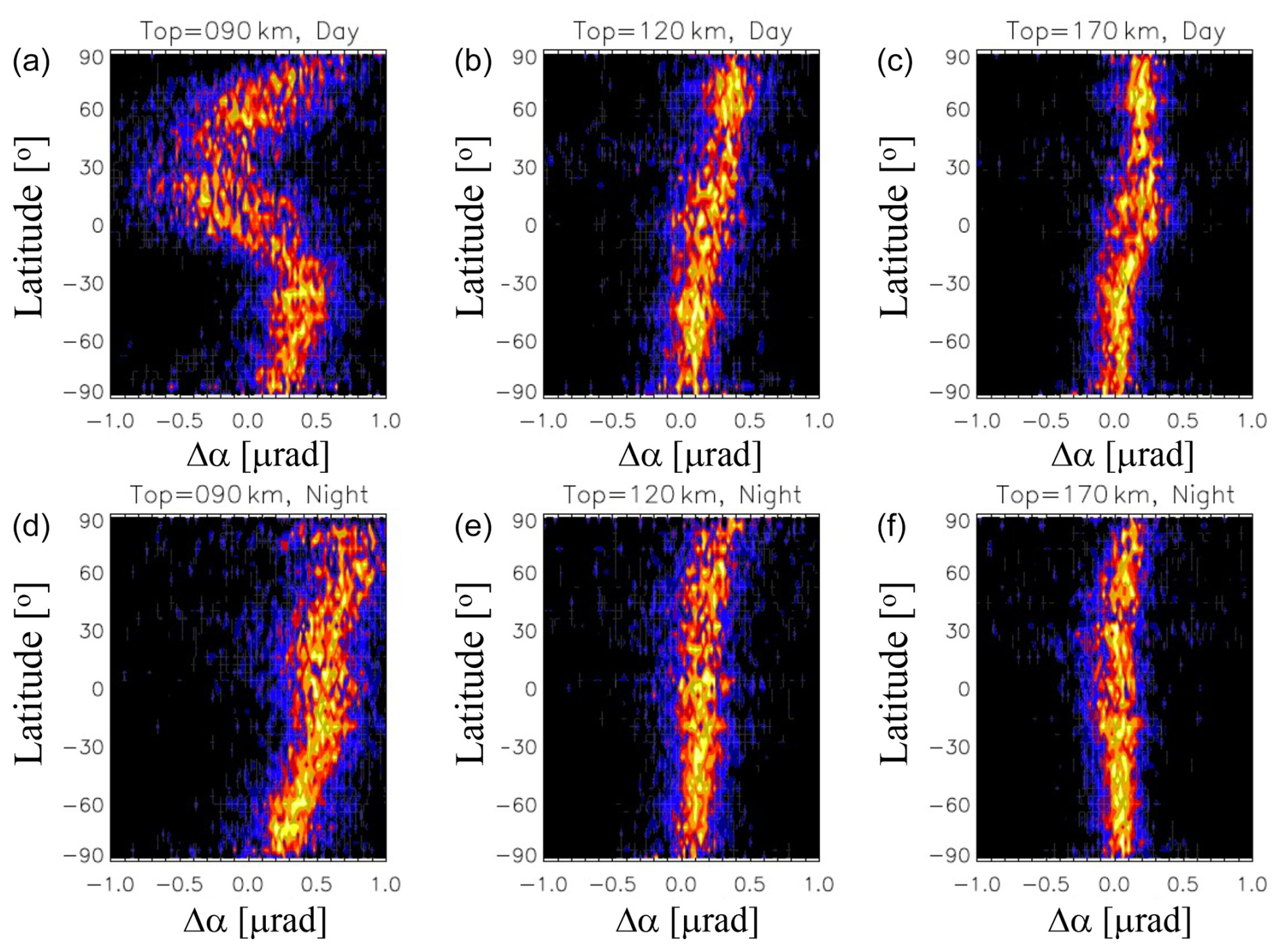
Figure 16 Probability distribution function (PDF) of the RIE derived from the $-\mathrm{d}{\mathit{\varphi }}_{\mathrm{ex}}/\mathrm{d}{h}_{\mathrm{t}}$ algorithm to compare impacts of the RO top-height truncation. The experimental data from the MetOp-A special scan during D161–D254 in 2020 were used in the analysis, and the RIE statistics from day (top panels) and night (bottom panels) are reported separately. The RIE results from three RO cutoff top heights, 90, 120, and 170 km, are selected for comparisons.

As suggested by the results in Fig. 16, it is imperative to raise the RO sounding top to at least 120 km for the RIE estimation because the lower truncation height (90 km) exhibits an inconsistent RIE distribution compared to those obtained with higher truncation heights. The RIEs derived from the 120 and 170 km truncations have similar statistics for both day and night, suggesting that the 120 km truncation would be high enough to overcome the potential Es influence on the RIE calculation. As shown in Fig. 2c, the $\mathrm{d}{\mathit{\varphi }}_{\mathrm{ex}}/\mathrm{d}{h}_{\mathrm{t}}$ method would suffer from the Es tail below the Es layers. Providing a few RO measurements above the Es layer would substantially help to constrain $\mathrm{d}{\mathit{\varphi }}_{\mathrm{ex}}/\mathrm{d}{h}_{\mathrm{t}}$ for the RIE calculation. Therefore, the inconsistent statistics from the 90 km truncation, compared to those derived from a higher RO top, can be explained primarily as Es impacts. If one plans to use the $\mathrm{d}{\mathit{\varphi }}_{\mathrm{ex}}/\mathrm{d}{h}_{\mathrm{t}}$ method to estimate and correct the RIE, the RO top height as summarized in Appendix C becomes an important parameter to know for current and past missions. For past missions with an RO top lower than 120 km, it would require an RIE climatology built upon other missions that can be parameterized as a function of latitude, longitude, local time, and solar cycle.

5.3 RIE signatures from other methods

5.3.1 Deviation from the exponential profile

RIEs and their effects can be evaluated with other methods or comparative analyses by including an α bias against ground-based radar observations (Danzer et al., 2013) and α climatologies (Li et al., 2020). Here, we introduce a method that uses the height variation of the excess phase ϕ_ex profile in the upper stratosphere to compare it with the expected exponential lapse rate. Since α is related to ${\mathit{\varphi }}_{\mathrm{ex}}/\mathrm{d}{h}_{\mathrm{t}}$ (Eq. 6), the ϕ_ex profile contains information on the RIEs seen in α. It is shown in Melbourne et al. (1994) and Wu et al. (2022) that the iono-free ϕ_ex profile is proportional to

$$\begin{array}{}\text{(8)}& {\mathit{\varphi }}_{\mathrm{ex}}\left(h_{\mathrm{t}}\right)\approx \mathrm{1.8}\times {\mathrm{10}}^{-\mathrm{5}}\cdot N\left(h_{\mathrm{t}}\right)\sqrt{H\cdot R_{\mathrm{e}}},\end{array}$$

where N is atmospheric refractivity, H is the atmospheric scale height, and R_e is Earth's radius. Because the refractivity is proportional to air density, it tends to decrease exponentially with height, $N\left(h_{\mathrm{t}}\right)=N_{\mathrm{0}}{e}^{-(h_{\mathrm{t}}-h_{\mathrm{0}})/H}$, from a reference N₀ at height h₀. Hence, a departure from the exponential height dependence as described by Eq. (7) may be used to evaluate an RIE in the ϕ_ex profile.

Several lapse rate comparisons are shown in Fig. 17 where the ϕ_ex profile differences are highlighted in percentage from an exponential fit at heights above 40 km. The exponential model uses the data at 40–45 km for the fitting and extrapolates the model to the heights above and below. The model assumes a constant scale height at these altitudes, which may cause some errors if atmospheric temperature varies by 10 %–20 %. However, any large percentage departures would raise a concern and might indicate an RIE in the ϕ_ex profile. Since Eq. (5) cannot completely remove the ionospheric contribution, the departure from the exponential can be used to better the nature of these RIEs. As discussed above, ionospheric multipaths and horizontal–vertical gradients might play a significant role in the RIE of the ϕ_ex measurements.

Figure 17a is a typical case where the exponential model fits the ϕ_ex profile well up to ∼ 50 km but exhibits negative biases (observation minus model) at higher altitudes. These biases can be as high as 40 %–50 % at 50–60 km, much greater than 10 %–20 % typically seen at lower altitudes. It is possible that the low biases were caused by a colder atmosphere at higher altitudes compared to the temperature at 40–45 km because the scale height H is proportional to temperature and ϕ_ex is proportional to $\sqrt{H}\cdot e^{-(h_{\mathrm{t}}-h_{\mathrm{0}})/H}$ in Eq. (8). For example, explaining a 40% decrease in ϕ_ex would require the temperature to drop from 270 K at 45 km to 210 K at 55 km, which might be feasible with a very strong gravity wave.

Figure 17b illustrates a likely ionospheric effect where a sharp thin layer at ∼ 53 km creates a large disruption in terms of exponential dependence of ϕ_ex with height. The height dependence of ϕ_ex does not obey the normal exponential decrease as expected from the neutral atmosphere, but the departure from the exponential above the layer is also much lower by more than 50 %. It remains unclear why the layer is more disruptive at heights above than below. In other words, if such behavior is representative for the ionospheric effects of thin layers (e.g., Es), their RIEs on the neutral atmospheric measurements might be small.

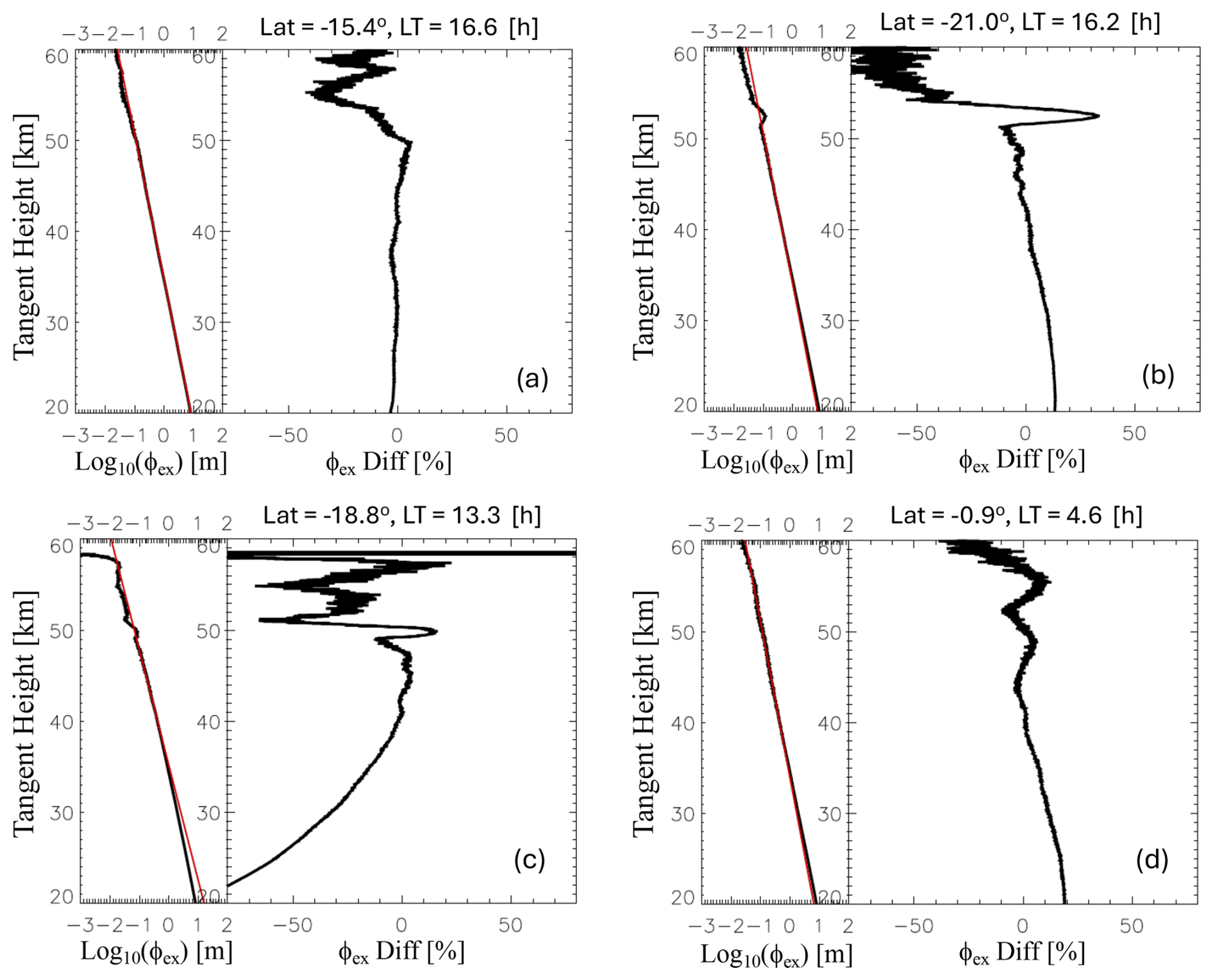
Figure 17 Examples of the departure of excess phase (ϕ_ex) measurements from an exponential fit (red line) at 40–45 km heights. The percentage difference between the observed and modeled ϕ_ex profile is displayed on the right as a function of tangent height. Selected cases are (a) typical negative departure from the exponential fit at higher altitudes, (b) departure from the exponential function due to a layered structure near 52–53 km, (c) largely different exponential dependence at heights above and below 40 km, and (d) wave-like oscillations at high altitudes. These cases were extracted from COSMIC-2 observations on 1 January 2022.

Figure 17c shows very different exponential dependences between the atmosphere below 40 km and above. To explain the 70 % difference using Eq. (8), one would have to assume a temperature difference of 120 K between 25 and 45 km. On the other hand, if a reference from the lower altitudes (e.g., 30 km) were used, it could help to reduce the biases in the lower atmosphere but would induce a much larger (> 100 %) bias at higher altitudes. In summary, this is a case likely caused by an RIE that can have a large departure of the ϕ_ex measurement from the expected exponential dependence with height. The biases above and below 40 km are too large to be explained by a normal atmosphere, but an RIE in the ϕ_ex measurement can certainly induce a large error like this.

Figure 17d displays a wave-like oscillation above 40 km in the bias from the exponential dependence. It perhaps reveals a real atmospheric gravity wave in the ϕ_ex measurement up to 60 km. If no RIE had impacted this profile, it would imply that the RO technique could provide good sensitivity to atmospheric temperature up to 60 km. Because RIEs can produce a local impact at a narrow height range, like Es, as well as an extended impact from the multipath propagation through the F-region, it remains a great challenge to distinguish between good cases like Fig. 20d and RIE-impacted cases like Fig. 20b.

5.3.2 Small-scale temperature variances

Variability of the GNSS-RO temperature profiles can also be used to infer potential RIE impacts, because additional fluctuations induced by RIEs can be as large as the RIE-induced bias. As shown in Fig. 10, the standard deviation of RIE Δα is often greater than the mean, suggesting that these RIE Δα variations might have propagated to the atmospheric temperature retrieval. Because ionospheric variability has a wide range of spatiotemporal scales (e.g., scintillation, Es), it is possible that small-scale RIE Δα variations may be not completely removed and result in artificial wave-like oscillations in the retrieved temperature profiles.

To evaluate RIE impacts on RO retrieval variability, we analyzed the entire MetOp-A/B/C record of temperature data produced by the Radio Occultation Meteorology Satellite Application Facility (ROM SAF) to extract small-scale variances using the algorithm developed previously for Es and gravity wave (GW) studies (Wu et al., 2005; Wu, 2006). This algorithm is similar to those used in other studies (e.g., Tsuda et al., 2000; Schmidt et al., 2008), except that we derived GW variances using a bandpass filter for a more careful treatment of the measurement noise. In the data analysis with this algorithm, each RO temperature profile T(z) is first processed with a running-window smoothing (truncation length Δz) to obtain a background ($\stackrel{\mathrm{‾}}{T\left(z\right)}$). The difference ($T\left(z\right)-\stackrel{\mathrm{‾}}{T\left(z\right)}$) is used to compute the variance for this truncation Δz. The minimum truncation length is defined by the three-point length in the temperature retrieval, which is ∼ 100 m in the upper troposphere and stratosphere and can be used to estimate the measurement noise on a profile-by-profile basis. The bandpass-filtered variance is defined as the variance difference between the Δz and the three-point truncation. The bandpass-filter method has been successfully applied to other satellite measurements for GW studies (Wu and Eckermann, 2008; Gong et al., 2012).

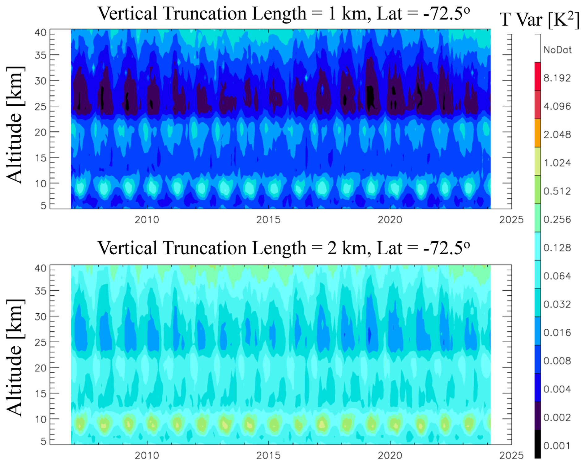
Figure 18 Time–height variation of the monthly small-scale variances derived from MetOp-A/B/C RO dry temperature retrievals at 72.5°.

Figure 18 shows a time series of monthly MetOp temperature variances derived with the bandpass-filter method for truncations of 1 and 2 km at 72.5°. A significant solar cycle variation is evident in the temperature variances, particularly in the upper stratosphere, which suggest that RIE impacts might have an amplitude of 0.03 and 0.3 K² in the 1 and 2 km variances at ∼ 40 km altitude. Similar solar cycle variation exists in the northern high latitudes (not shown) with a comparable amplitude, but the solar cycle dependence becomes less pronounced at low latitudes. It is expected that the RIE impacts would be greater at high latitudes, as revealed in the DA impact study (Sect. 4.3). Although the solar-cycle-dependent temperature variations do not provide a direct indication of whether the RO temperature is artificially biased by a solar cycle influence, earlier studies have found such bias evidence (Danzer et al., 2013; Li et al., 2020).

6 Conclusions

In this study we developed an empirical algorithm to estimate the RO residual ionospheric error (RIE) from the vertical gradient of excess phase (ϕ_ex) measurements at h_t>65 km. The method, called the $\mathrm{d}{\mathit{\varphi }}_{\mathrm{ex}}/\mathrm{d}{h}_{\mathrm{t}}$ method, is self-sufficient and based on the empirical linear fit to the ϕ_ex data on a profile-by-profile basis. The RIE estimation does not rely on any auxiliary data or model sources. $\mathrm{d}{\mathit{\varphi }}_{\mathrm{ex}}/\mathrm{d}{h}_{\mathrm{t}}$ is a good measure of α at high h_t (if there is a bending), but it also contains errors induced by other factors from the radio wave propagation in an inhomogeneous ionosphere such as higher-order frequency dependence. The derived RIE is extrapolated to the RO measurements at the lower h_t, assuming that the entire α profile is impacted by error Δα.

Although the derived RIE (Δα) is dominated by positive values, the $\mathrm{d}{\mathit{\varphi }}_{\mathrm{ex}}/\mathrm{d}{h}_{\mathrm{t}}$ method also produces negative values for both day and night. This is fundamentally different from the κ method that only produces a positive RIE. Diurnal variations of the RIE Δα are latitude- and LST-dependent with larger negative amplitudes (up to −3 µrad) in the daytime tropics and subtropics. The standard deviations of RIE Δα can be greater than their mean values in the climatology averaged by LST and latitude. Significant solar cycle and longitudinal variations are found in the RIE Δα derived from observations. The dependence of RIE on the geomagnetic field is evident but relatively weak compared to the diurnal and geographical variabilities.

RIE impacts on data assimilation (DA) were evaluated with experiments using the NASA GMAO Goddard Earth Observing System (GEOS) that assimilates GNSS-RO α data for MERRA-2. An LST latitude-varying Δα bias similar to the COSMIC-1 RIE climatology was added to the RO data in the GEOS-IT DA experiments. The RIE impacts on the DA temperature were found mostly in the polar stratosphere with a bias as large as 2–4 K at 1 hPa and ∼ 1 K at 10 hPa. There is a small (±0.3 K) temperature bias in the troposphere. The diurnally varying RIE does not appear to impact the migrating tides in the upper stratosphere and mesosphere because the tidal waves are locked to the solar forcings from the lower atmosphere.

The $\mathrm{d}{\mathit{\varphi }}_{\mathrm{ex}}/\mathrm{d}{h}_{\mathrm{t}}$ method requires the RO profile to reach at least 120 km to minimize the sporadic-E (Es) layer influences. Es occurs mostly at 90–110 km with a strong localized effect in this altitude range, but its tailing effect can extend far below the Es layers in the RO ϕ_ex profile. Additional constraints from the RO measurements at 120 km and above would help to suppress the Es influences and provide a more accurate estimate of the RIE from the F-region ionosphere.

RIEs were also found in the RO ϕ_ex measurements by comparing the observed profile with an expected exponential decrease with height. In addition, the RIE impacts can be seen in the small-scale variance of RO temperature retrievals. In both cases, the RIE amplitudes appear to increase with height and become a significant source of error in the upper stratosphere. The findings from this study further emphasize the need to treat RIEs carefully, especially with the growing infusion of commercial GNSS-RO data for climate studies.

Appendix A: Bending delay and phase advance

The radio wave propagation in GNSS-RO can have an excess phase ϕ_ex from both bending delay and phase advance. These opposite effects in ϕ_ex are often confused in the literature because they both have the same first-order dependence on f⁻². The bending effect increases the propagation path length and induces a delay in the excess phase measurements (ϕ_exL1 or ϕ_exL2) because of the group velocity of radio waves. Although the group velocity is equal to or less than the light speed, the phase velocity of radio wave propagation in plasma can exceed the light speed, causing a phase advance in ϕ_exL1 or ϕ_exL2. Two competing effects coexist in the GNSS-RO observations, and both are evident in the E-region ϕ_exL1 and ϕ_exL2 measurements shown in Wu (2018). In these RO ϕ_exL1 and ϕ_exL2 profiles, the F-region effect manifests itself primarily as a phase delay that varies gradually with h_t, while the phase advance from narrow sporadic-E layers is superimposed on the F-region variation.

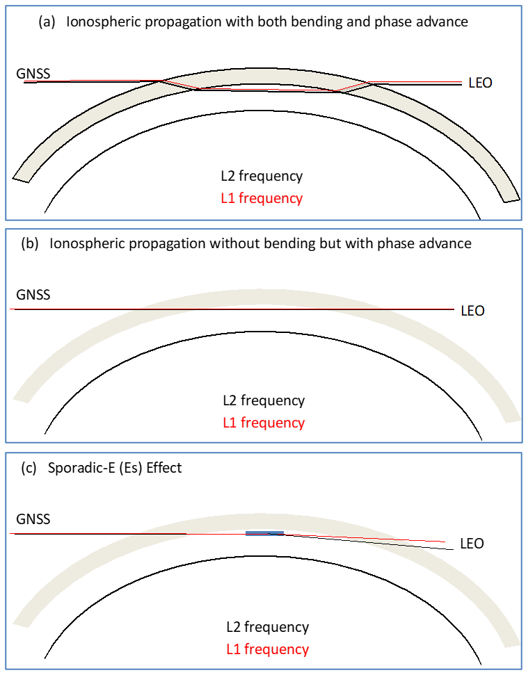
Figure A1 Illustration of radio wave propagation through an idealized ionosphere (a) with and (b) without bending. A sharp vertical gradient in ionospheric electron density can induce a significant bending, whereas the bending is small and negligible if the gradient is weak. The case in panel (a) illustrates the bending from a sharp refractivity gradient between the vacuum and an ionospheric layer. The case in panel (b) assumes a smooth and gradual transition between the vacuum and the ionosphere such that bending is negligible. In both cases the phase advance is significant and non-negligible (see the text for more description).

Because path length changes and phase advances are coupled in GNSS-RO, especially for the radio wave propagation with a long path through a structured ionosphere, quantifying their relative importance in RIE is not trivial. Figure A1 highlights the differences between bending-induced delay and plasma phase advance using an idealized geometry with and without bending. The bending can be upward and downward in the F-region, as the radio wave propagates across an interface with a large refractivity gradient (Fig. A1a). The bending induces a path length change in the L1 and L2 propagation and a subsequent phase delay. However, this delay is offset in the meantime by the phase advance from the radio propagation in plasma. The net effect would depend on how significant the bending is. In the case with little or insignificant bending, as in Fig. A1b, a phase advance still exists and could be misinterpreted as an upward bending even though there is no bending. For a typical Chapman-layer ionosphere, Hoque and Jakowski (2011) found that the bending-induced ϕ_exL1 error is about 1–2 m for the L1 frequency, while the phase advance over a long path length can be as high as tens of meters or over 100 TECu (1 TECu = 0.162 m for L1).

Appendix B: RIE impacts on mesospheric temperature and winds

Solar migrating tides dominate the diurnal variation in the upper-atmospheric temperature and winds. Thus, it is imperative to assess the relative importance of RIE impact as a function of local time. Figures B1–B2 show the local time variations of temperature at 1 and 0.1 hPa where the GNSS-RO RIE errors can be very large compared to the mean α. Interestingly, the local time variations from experiments NoGPS and BiasLST look very similar to that from the control experiment, despite large differences in the zonal mean temperatures. The experiment with a very large bias (BiasM2) appears to dampen the diurnal amplitude by 30 %–50 %. Otherwise, the experiments with NoGPS and BiasLST do not seem to significantly change the tidal phase in LST because the dominant migrating tidal modes are locked in phase with the solar forcings in the troposphere and stratosphere.

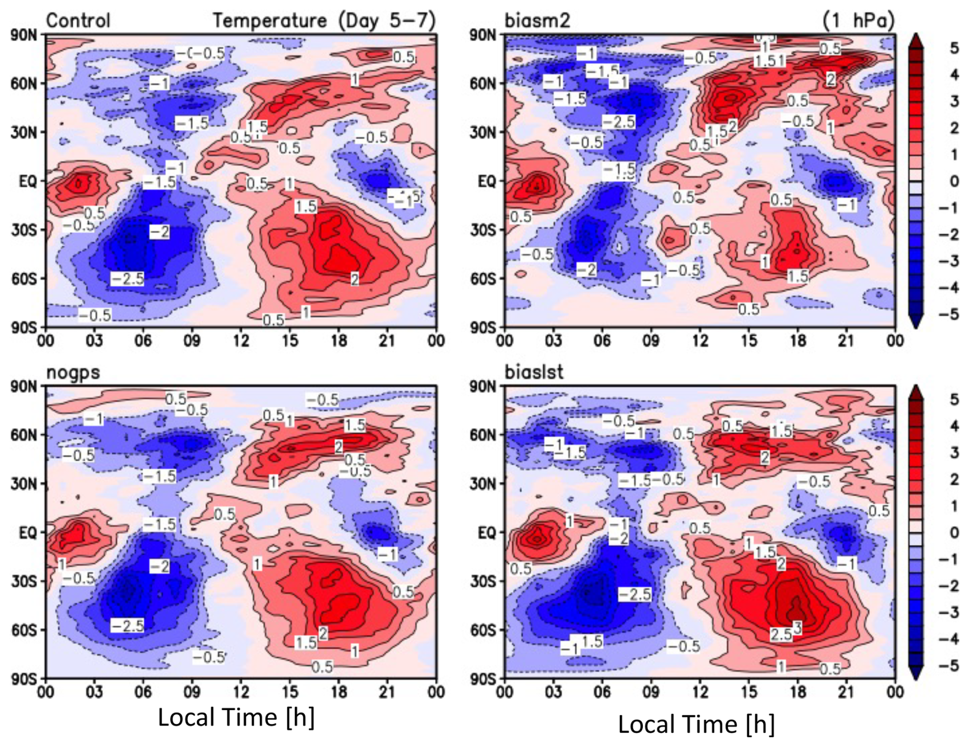
Figure B1 Diurnal temperature variations from the controlled and perturbed experiments at 1 hPa. The temperature perturbations from the zonal mean in Kelvin are contoured in color.

Despite a relaxed value used in the DA covariance matrix in assimilating GNSS-RO α from higher altitudes, the measurement errors such as RIE still have a significant impact on the assimilated winds and temperatures at pressures < 5 hPa. For example, in Fig. B3 the CTL–NoGPS difference suggests that the GNSS-RO data made an equatorward shift of the polar vortex near 0.2 hPa in the Northern Hemisphere winter. In the presence of an RIE like BiasLST, this shift becomes larger at pressures > 0.2 hPa but in the poleward direction at < 0.2 hPa. In the Southern Hemisphere, the BiasLST makes the zonal winds shifted significantly equatorward. Because the reanalysis data have been widely used at these pressure levels (1–0.1 hPa), the RIE impact needs to be carefully evaluated for the period when GNSS-RO data are assimilated.

Figure B2 As in Fig. B1 but for 0.1 hPa.

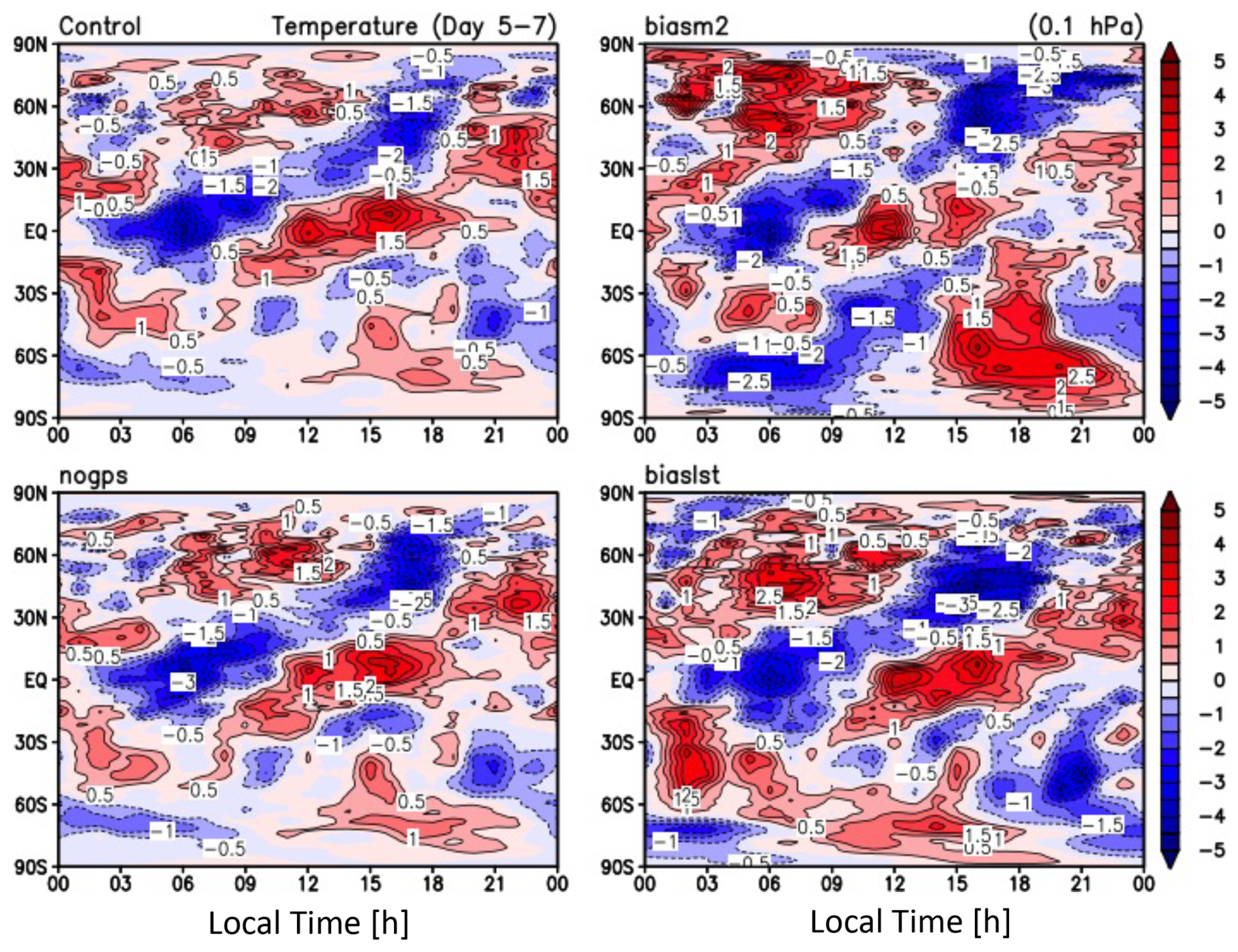
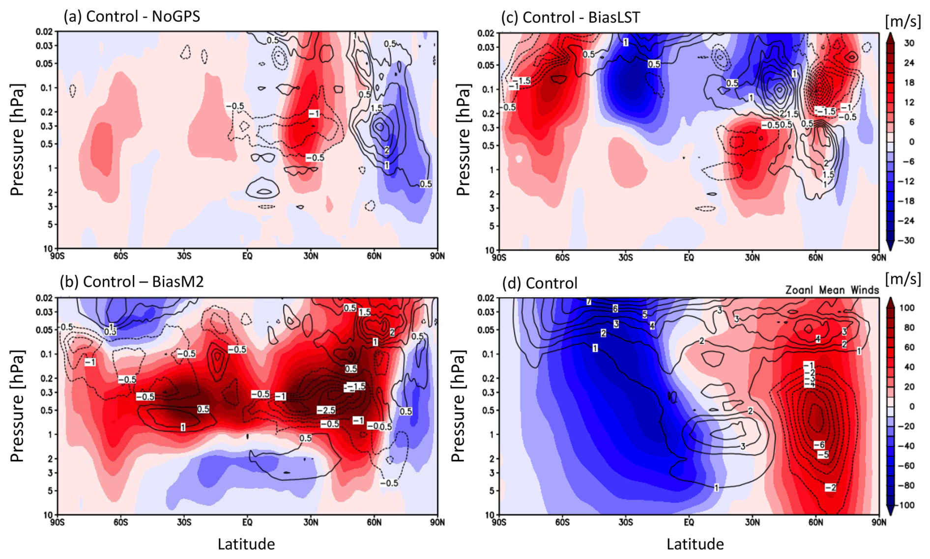
Figure B3 Impacts of the RIEs on upper-atmospheric winds at 10-0.02 hPa from the DA experiments: (a) CTL–NoGPS, (b) CTL–BiasM2, and (c) CTL–BiasLST, sharing the same color scale in panel (c). The mean wind from CTL is displayed in (d). All panels have the zonal winds contoured in color with units of m s⁻¹, superimposed by the meridional winds contoured by lines.

Appendix C: GNSS-RO mission summary

The global GNSS-RO observations can perhaps be divided into three periods in terms of the total number of daily RO profiles: CHAMP period (2001–2006), COSMIC1 period (2006–2019), and COSMIC2 commercial period (2019–present). Advances in commercial RO receiver technologies play a critical role in the increase in the number of RO acquisitions from space in recent years. The BlackJack RO receiver on CHAMP, developed by the NASA Jet Propulsion Laboratory (JPL), was able to track dual-frequency GPS (G) signals for precise (centimeter accuracy range) orbit determination and continuous coverage (Hajj et al., 2004). For the RO observation, the receiver software was also able to schedule high-rate (50 Hz) tracking of setting occultations of up to four GPS satellites. The BlackJack on CHAMP has only aft antennas for the RO sounding, which yielded ∼ 250 profiles per day. The sampling was further improved by tracking rising occultations with the open-loop (OL) tracking successfully demonstrated on the SAC-C and later COMSIC-1 satellites. This advance led to the dual-antenna (aft and fore) and OL tracking IGOR (Integrated GPS and Occultation Receiver) implemented by the COMSIC-1 constellation (BRE, 2003), which produced ∼ 700 daily ROs per satellite, or an average total of ∼ 4000 daily ROs from a six-satellite constellation.

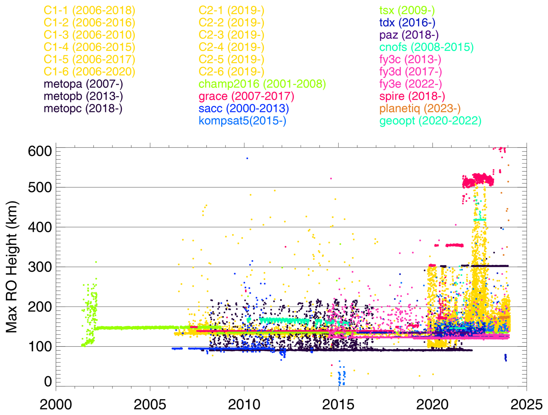
Figure C1 Daily GNSS-RO statistics of the maximum RO top height from the past and current missions in 2001–2023.

Table C1 Summary of GNSS-RO data used in this study.

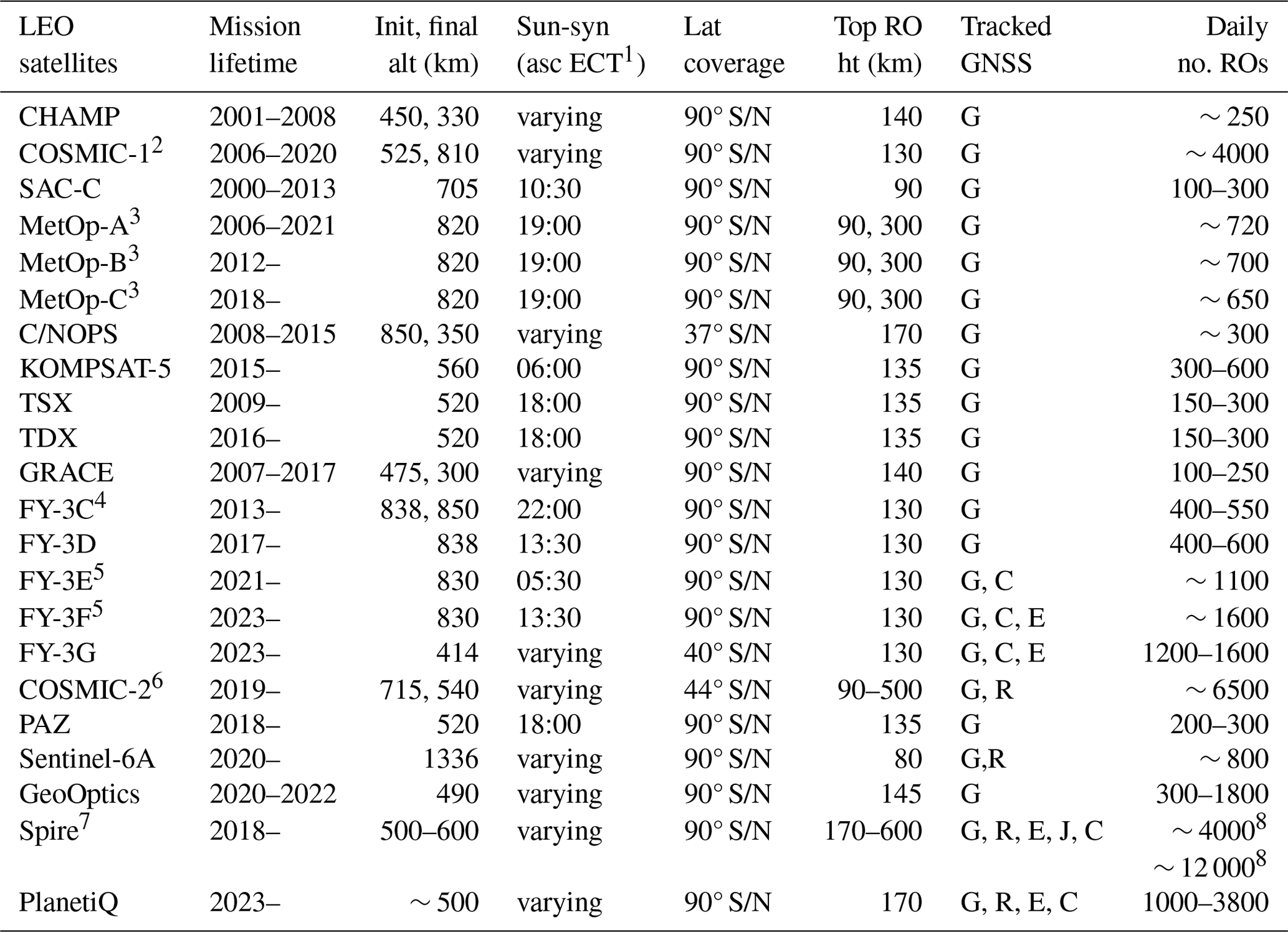
¹ Ascending-orbit Equator crossing time (asc ECT). ² The COSMIC1-3 spacecraft never reached the intended orbital altitude and was operated at 725 km for the rest of its mission. ³ MetOp-A started to drift away from the Sun-sync orbit in ∼ 2021. An extended RO experiment with MetOp-A acquired high-rate data up to h_t=300 km during 2020D161–2020D254. Following the successful experiment, the high-top RO acquisition has been implemented for routine operation in MetOp-B/C since 2021. ⁴ FY-3C started to drift away from the Sun-sync orbit (SSO) in 2016. ⁵ FY-3E started to track GPS (G) and BDS (C), and FY-3F and 3G started to track GPS (G), BDS (C), and Galileo (E) ⁶ The CDAAC COSMIC-2 NRT data contain GNSS-RO profiles from GPS (G) and GLONASS (R). The nominal RO top is ∼ 140 km, but it occasionally reaches up to 300 or 500 km for space weather measurements. ⁷ The Spire GNSS-RO observation tracks GPS (G), GLONASS (R), Galileo (E), and BDS (C) signals routinely to ∼ 170 km, but for space weather observations the tracking often goes up to 300, 350, 500, or 600 km. The tracking of and QZSS (J) occurred briefly before 2021. ⁸ NASA's Commercial Smallsat Data Acquisition (CSDA) data have a larger number of post-processing RO profiles per day from November 2019 to the present. The NOAA Commercial Data Program (CDP) acquires fewer near-real-time (NRT) RO profiles per day compared to the CSDA archive.

The recent boost in the number of GNSS-RO observations, as shown in Fig. C1, came from the availability of civil signals provided by GNSS satellites (GLONASS – R, Galileo – G, and BDS – C) and from the combination of a new four-antenna TriG (Tri-band GNSS) receiver (Esterhuizen et al., 2009) on COSMIC-2 and commercial CubeSat constellations. While operational weather satellites such as MetOp (Zus et al., 2011) and FY3 (Bai et al., 2014) continue to provide global GNSS-RO observations, the commercial data from SmallSat/CubeSat constellations provided by Spire (Angling et al., 2021), GeoOptics (Chang et al., 2022), and PlanetiQ (Kursinski et al., 2021) have become increasingly important to yield the needed spatiotemporal coverage on the globe. The maximum RO top height, listed in Table C1 for these missions, is a key parameter to derive the RIE with the $\mathrm{d}{\mathit{\varphi }}_{\mathrm{ex}}/\mathrm{d}{h}_{\mathrm{t}}$ method presented in this study.