ScintPi measurements of low-latitude ionospheric irregularity drifts using the spaced-receiver technique and SBAS signals

Previous efforts have used pairs of closely spaced specialized receivers to measure Global Navigation Satellite System (GNSS) signals and to estimate ionospheric irregularity drifts. The relatively high cost associated with commercial GNSS-based ionospheric receivers has somewhat limited their deployment and the estimation of ionospheric drifts. The development of an alternative, low-cost, GNSS-based scintillation monitor (ScintPi) motivated us to investigate the possibility of using it to overcome this limitation. ScintPi monitors can observe signals from geostationary satellites, which can greatly simplify the estimation of the drifts. We present the results of an experiment to evaluate the use of ScintPi 3.0 to estimate ionospheric irregularity drifts. The experiment consisted of two ScintPi 3.0 deployed in Campina Grande, Brazil (7.213° S, 35.907° W; dip latitude ∼ 14° S). The monitors were spaced at a distance of 140 m in the magnetic east–west direction and targeted the estimation of the zonal drifts associated with scintillation-causing equatorial spread F (ESF) irregularities. Routine observations throughout an entire ESF season (September 2022–April 2023) were made as part of the experiment. We focused on the results of irregularity drifts derived from geostationary satellite signals. The results show that the local time variation in the estimated irregularity zonal drifts is in good agreement with previous measurements and with the expected behavior of the background zonal plasma drifts. Our results also reveal a seasonal trend in the irregularity zonal drifts. The trend follows the seasonal behavior of the zonal component of the thermospheric neutral winds as predicted by the Horizontal Wind Model (HMW14). This is explained by the fact that low-latitude ionospheric F-region plasma drifts are controlled, in great part, by Pedersen-conductivity-weighted flux-tube-integrated zonal neutral winds. The results confirm that ScintPi has the potential to contribute to new, cost-effective measurements of ionospheric irregularity drifts, in addition to scintillation and total electron content. Furthermore, the results indicate that these new ScintPi measurements can provide insight into ionosphere–thermosphere coupling.

1 Introduction

A series of low-cost, easy-to-install and easy-to-maintain ionospheric scintillation and total electron content (TEC) monitors were developed at The University of Texas at Dallas (UT Dallas; e.g., Rodrigues and Moraes, 2019; Gomez Socola and Rodrigues, 2022). These monitors are referred to as ScintPi and were developed using commercial off-the-shelf (COTS) Global Navigation Satellite System (GNSS) receivers and single-board computers (Raspberry Pi). While ScintPi monitors were not developed to fully replace commercial monitors, they can be used for various scientific and educational applications. For instance, ScintPi monitors have been successfully used in studies of ionospheric irregularities and TEC depletions at low latitudes and at the region of transition between low and middle latitudes (e.g., Sousasantos et al., 2023, 2024; Gomez Socola et al., 2023). ScintPi monitors have also been used in studies of solar radio bursts and their impact on GNSS signals (Wright et al., 2023a) and in student projects related to space weather (Wright et al., 2023b).

Given that ScintPi has a reduced sampling rate (20 Hz) and carrier-to-noise ratio (C$/$No) resolution (1 dB-Hz) compared with typical commercial scintillation monitors, the ability of ScintPi to produce satisfactory drift estimates needed to be investigated. On the other hand, ScintPi is capable of monitoring signals transmitted by geostationary satellites, which would greatly simplify the analyses associated with and interpretation of irregularity drift measurements.

Therefore, here, we present the results of an experimental effort to evaluate the use of ScintPi monitors to estimate ionospheric irregularity drifts. The approach follows that of the so-called closely spaced scintillation technique, which measures time differences between the occurrence of scintillation patterns observed by closely spaced receivers to infer the horizontal velocity component of scintillation-causing irregularities along the receivers' baseline.

Ionospheric plasma drifts represent an important feature of the ionospheric plasma behavior and are responsible for controlling plasma transport and structuring. For instance, vertical (upward) F-region plasma drifts drive the transport of plasma from the magnetic equator to low latitudes through the ionospheric plasma fountain effect (Hanson and Moffett, 1966; Moffett, 1979). This mechanism gives rise to the Equatorial Ionization Anomaly – EIA (Appleton, 1946; Bailey, 1948). Additionally, the so-called pre-reversal enhancement (PRE) in vertical drifts, occurring near sunset, is known to control the development of the equatorial spread F – ESF (Heelis et al., 1974; Farley et al., 1986; Fejer et al., 1999; Fesen et al., 2000).

The magnetic zonal component of the F-region plasma velocity at low latitudes, on the other hand, can reflect the level of coupling between the upper thermosphere and ionosphere (Immel et al., 2006; Wang et al., 2021). During nighttime, the E-region dynamo is greatly reduced, and F-region plasma drifts should reflect the effects of the F-region dynamo alone (e.g., Coley et al., 1994).

Ionospheric plasma drifts are also relevant for certain applications. According to Carrano and Groves (2010), the probability of experiencing loss of lock and likelihood of extended signal reacquisition times depend on factors such as the velocity of the satellite motion with respect to the geomagnetic field and plasma drifts.

Obtaining ground-based measurements of background ionospheric plasma drifts presents significant challenges. For instance, the incoherent scatter radar (ISR) of the Jicamarca Radio Observatory (JRO) is the only instrument capable of making observations of vertical and zonal plasma drifts. While the measurements can be conducted across various heights within the F region, the observations require the operation of high-power transmitters, limiting the number of measurements per year.

The motion of ionospheric irregularities can be measured more easily than the motion of the background ionospheric plasma using, for instance, L-band spaced scintillation receivers (Kil et al., 2000, 2002; Ledvina et al., 2004; Kintner et al., 2004; Kintner and Ledvina, 2005; Cerruti et al., 2006; Otsuka et al., 2006; Sobral et al., 2009; de Paula et al., 2010; Muella et al., 2008, 2009, 2013, 2014, 2017; Cesaroni et al., 2021). Irregularity drifts are often used as an indicator of background plasma drifts at low latitudes. The application of the scintillation-based spaced-receiver technique to measure irregularity drifts is revisited in this study, with a focus on using more cost-effective instrumentation for the measurements.

Gomez Socola and Rodrigues (2022) have already addressed the ability of the sampling rate (20 Hz) and amplitude resolution (1 dB-Hz) of ScintPi 3.0 measurements to produce amplitude scintillation indices that are comparable to those produced by commercial GNSS-based monitors. Here, we present the results of an experimental setup and campaign that targeted an evaluation of the application of the scintillation-based spaced-receiver technique to ScintPi 3.0 measurements and the estimation of irregularity drifts.

The presentation of our work is organized as follows: in Sect. 2, we provide information about the ScintPi 3.0, measurements, spaced-receiver experimental setup and geophysical conditions under which measurements were made; Sect. 3 describes the methodology used to derive irregularity drifts from the ScintPi measurements; in Sect. 4, we present and discuss the results of the measurements and analyses; and Sect. 5 summarizes our main findings.

2 Experimental setup

Scintillation observations were carried out using ScintPi 3.0 monitors. ScintPi 3.0 can be described as a multi-GNSS-constellation, dual-frequency ionospheric scintillation and TEC monitor. ScintPi was developed at UT Dallas using a COTS GNSS receiver and a single-board computer (Raspberry Pi).

The development of ScintPi was motivated by the relatively high cost of commercial GNSS-based scintillation and TEC monitors. While it is not intended to fully replace commercial monitors, ScintPi allows different research and educational initiatives. Details about ScintPi 3.0, along with illustrative examples of measurements and comparison with co-located observations made by commercial receivers, are described in Gomez Socola and Rodrigues (2022). Examples of different types of studies using ScintPi measurements can be found in Gomez Socola et al. (2023), Sousasantos et al. (2023, 2024) and Wright et al. (2023a). Results of an educational effort using ScintPi can be found in Wright et al. (2023b). Of relevance to this study is that ScintPi can measure the strength of signals transmitted by GNSS satellites, achieving sampling rates of 20 Hz and a C$/$No resolution of 1 dB-Hz. In this study, our focus centers on the analysis of signals transmitted by geostationary satellites. The use of geostationary satellites simplifies the analyses and the interpretation of the measurements.

2.1 Deployment and spacing

Because low-latitude equatorial plasma bubbles (EPBs) and the ionospheric irregularities associated with them are known to move in the magnetic zonal direction (Dyson and Benson, 1978; Mendillo and Baumgardner, 1982; Martinis et al., 2003, 2020), the two monitors were placed at a distance of 140 m from one another along the east–west magnetic direction. The site is in a region of −21.39° magnetic declination based on magnetic values from the International Geomagnetic Reference Field – IGRF-13 (Alken et al., 2021) (see Fig. 1b). The spacing was chosen based on expected values of low-latitude irregularity drifts, the sampling rate of the receivers and the availability of locations. The sampling rate of the receivers (or sampling frequency, f_s), the spacing between receivers (d) and the apparent component of the irregularity velocity along the baseline ($v_{\mathrm{scint}}^{\prime }$) dictate the delay (in samples, N ∼ $f_{\mathrm{s}}d/v_{\mathrm{scint}}^{\prime }$) between the two patterns observed by the spaced receivers. Additional details will be provided in Sect. 3. Figure 1a shows the location of the observation site (UFCG). Figure 1b and c describe the placement of the receivers.

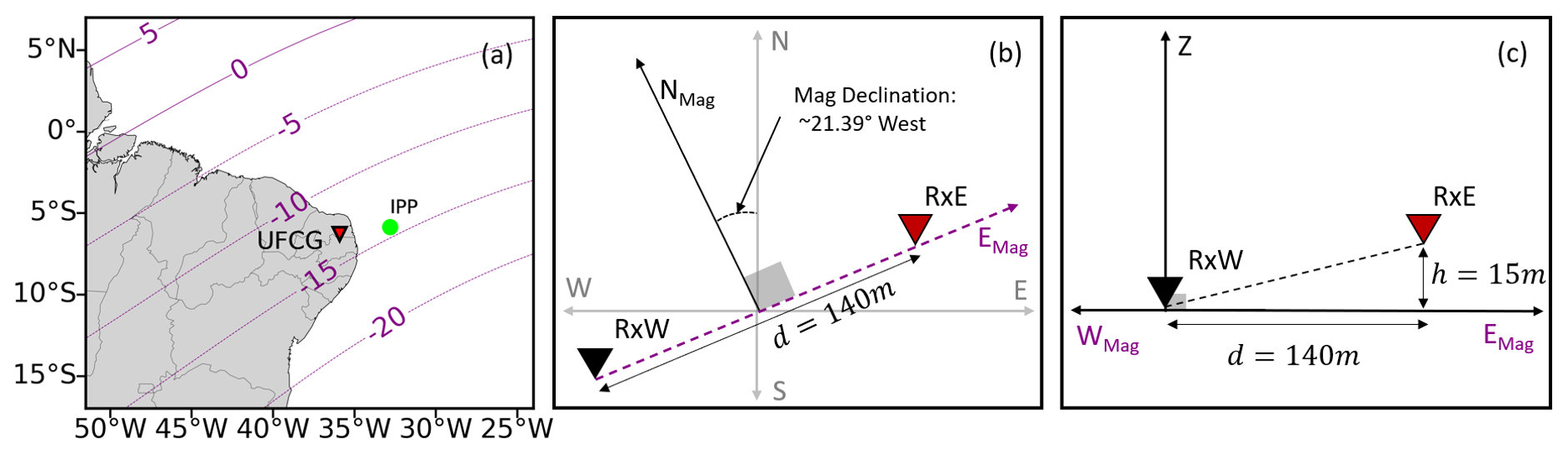
Figure 1 (a) Map showing the location of UFCG, where spaced ScintPi 3.0 monitors were deployed for this study. UFCG is located at ∼ 14° dip latitude, where L-band scintillations occur frequently. Panels (b) and (c) are diagrams showing the placement of the monitors along the magnetic zonal direction for the estimation of ionospheric irregularity drifts using the scintillation-based spaced-receiver technique.

2.2 Measurements

While ScintPi 3.0 can make measurements of signals transmitted by different GNSS satellites (GPS, GLONASS, BeiDou and Galileo), in this study we focused on measurements of signals transmitted by geostationary satellites which can also be measured by ScintPi 3.0. The use of geostationary signals has various advantages. For instance, signals from geostationary satellites provide observations over a fixed location, allowing for unambiguous interpretation of the variability in the observed drifts. Additionally, the decorrelation times of the observed signal fluctuations are not affected by satellite velocities. Perhaps more importantly, the satellite velocity does not have to be considered in the analyses and calculations of ionospheric irregularity drifts.

The signals recorded by GNSS receivers are coded using pseudo-random noise (PRN) sequences, which are codes that each satellite transmits to differentiate itself from other satellites. At the location of UFCG, ScintPi 3.0 monitors can decode signals from the Astra 5B (PRN123) and Astra SES-5 (PRN136) geostationary satellites, stationed at 31.5 and 5° E geographic longitudes, respectively. Unfortunately, data from PRN123 had to be excluded due to its low elevation angle (∼ 14°), which led to non-geophysical amplitude fading caused by multipath effects. PRN136, on the other hand, was positioned at an elevation angle of 42° and azimuth of 84° which provided adequate measurements for this study. The ionospheric pierce point (IPP) for the PRN136 signal is located at 6.77° S, 31.86° W (dip latitude ∼ 15° S), as shown in Fig. 1a. The IPP calculation followed the method outlined by Prol et al. (2017), considering the altitude of the ionospheric F-region peak density at 450 km.

For this study, we analyzed 8 months (1 September 2022–30 April 2023) of nearly continuous measurements. The measurements covered an entire ESF season in Brazil, when scintillations occur frequently. The measurements were made during the ascending phase of solar cycle 25, and the mean solar flux for the period was 148.23 SFU (where SFU denotes solar flux units).

3 Scintillation pattern velocities and ionospheric irregularity drifts

As previously mentioned, ScintPi 3.0 measures the strength of L-band signals transmitted by geostationary satellites. These signals are subject to diffraction by irregularities in the ionospheric plasma density, giving rise to intensity fading (scintillation) patterns observed by monitors on the ground.

At low magnetic latitudes, ionospheric irregularities are known to be elongated along the magnetic field lines and to drift in the zonal magnetic direction (Dyson and Benson, 1978; Mendillo and Baumgardner, 1982; Martinis et al., 2003, 2020). Therefore, an approach to estimate zonal irregularity drift is to measure the scintillation pattern velocity using receivers that are spaced in the magnetic zonal direction.

An experimental setup commonly used to measure the scintillation pattern velocity relies on the estimation of the time delay between scintillation patterns observed by spaced scintillation receivers. This time delay is quantified by the time lag at which the cross-correlation function of the measured signals reaches its maximum (τ₀). The measured (or apparent) scintillation velocity along the receiver baseline (${\mathit{\nu }}_{\mathrm{scint}}^{\prime }$) is then quantified from ${\mathit{\nu }}_{\mathrm{scint}}^{\prime }=d/{\mathit{\tau }}_{\mathrm{0}}$, where d represents the spacing between the receivers (Kil et al., 2000).

In this study, we consider the approach introduced by Briggs et al. (1950) which compensates for the temporal evolution of the intensity pattern. This approach is known as the “full correlation method” and has been widely used in the estimation of irregularity drifts (e.g., Kil et al., 2000; Kintner et al., 2004; Kintner and Ledvina, 2005; Otsuka et al., 2006; Sobral et al., 2009; de Paula et al., 2010; Muella et al., 2008, 2009, 2013, 2014, 2017). We summarize the approach in the following paragraphs.

Briggs et al. (1950) pointed out that the apparent velocity (${\mathit{\nu }}_{\mathrm{scint}}^{\prime }$) has a contribution from the random-like evolution of scintillation-causing irregularities as they move between the line of sight of the two observing receivers. The apparent velocity can be related to the true velocity (ν_scint) through the following expression (Briggs et al., 1950):

$$\begin{array}{}\text{(1)}& v_{\mathrm{scint}}={\displaystyle \frac{v_{\mathrm{scint}}^{\prime }}{\mathrm{1}+t_{\mathrm{0}}^{\mathrm{2}}/{\mathit{\tau }}_{\mathrm{0}}^{\mathrm{2}}}},\end{array}$$

where t₀ is the so-called characteristic time and is the time at which the autocorrelation of the scintillation pattern matches the maximum cross-correlation value. This time is associated with a random component in the motion of the plasma density irregularities; therefore, the ratio $t_{\mathrm{0}}^{\mathrm{2}}/{\mathit{\tau }}_{\mathrm{0}}^{\mathrm{2}}$ determines the extent to which the apparent and the true velocity are equivalent. For instance, when random motion (decorrelation) is negligible, the cross-correlation value for the two scintillation patterns approaches 1. As a result, t₀ will approach 0 and the ratio $t_{\mathrm{0}}^{\mathrm{2}}/{\mathit{\tau }}_{\mathrm{0}}^{\mathrm{2}}$ will be negligible. The measured velocity would then match the true velocity (v_scint ∼ $v_{\mathrm{scint}}^{\prime }$). In contrast, situations where t₀ and $t_{\mathrm{0}}^{\mathrm{2}}/{\mathit{\tau }}_{\mathrm{0}}^{\mathrm{2}}$ depart from 0 indicate that the scintillation pattern velocity has non-negligible contributions from random motion (Kintner et al., 2004). Finally, to quantify the contribution from random motions to the observed velocities, Briggs et al. (1950) introduced the so-called characteristic velocity (ν_c):

$$\begin{array}{}\text{(2)}& {\mathit{\nu }}_c=v_{\mathrm{scint}}\left({\displaystyle \frac{t_{\mathrm{0}}}{{\mathit{\tau }}_{\mathrm{0}}}}\right)={\displaystyle \frac{{\mathit{\nu }}_{\mathrm{scint}}^{\prime }}{\mathrm{1}+t_{\mathrm{0}}^{\mathrm{2}}/{\mathit{\tau }}_{\mathrm{0}}^{\mathrm{2}}}}\left({\displaystyle \frac{t_{\mathrm{0}}}{{\mathit{\tau }}_{\mathrm{0}}}}\right).\end{array}$$

Combining Eqs. (1) and (2), one can write the following:

$$\begin{array}{}\text{(3)}& v_{\mathrm{scint}}^{\prime }=v_{\mathrm{scint}}+{\displaystyle \frac{v_{\mathrm{c}}^{\mathrm{2}}}{v_{\mathrm{scint}}}}.\end{array}$$

Equation (3) shows, more explicitly, that the measured pattern velocity ($v_{\mathrm{scint}}^{\prime }$) has contributions from the true irregularity drifts and from the random characteristic irregularity velocity.

Figure 2 illustrates the estimation of τ₀ and t₀ used to compute true velocities (Eq. 1) and characteristic velocities (Eq. 2). Figure 2a shows a 60 s interval of signal strengths measured by the receivers at UFCG. Note that, despite the low C$/$No resolution (1 dB-Hz), similar fluctuations are observed by both receivers. Also note that fluctuations observed by the west receiver (RxW) precede the fluctuations observed by the east receiver (RxE), indicating eastward motion. Figure 2b shows the cross-correlation function between these two signals. From the maximum cross-correlation coefficient, we obtain the time delay (τ₀) needed to compute the apparent pattern velocity ($v_{\mathrm{scint}}^{\prime }$). Figure 2c shows the autocorrelation of the scintillation pattern measured by the west receiver. The maximum cross-correlation coefficient is used to estimate the characteristic time (t₀) (see the gray line in Fig. 2b and c). Again, we point out that, for high cross-correlation values (e.g., correlation coefficient ∼ 1), t₀ and $t_{\mathrm{0}}^{\mathrm{2}}/{\mathit{\tau }}_{\mathrm{0}}^{\mathrm{2}}$ would have negligible values, and the apparent velocity ($v_{\mathrm{scint}}^{\prime }$; Eq. 1) would converge to the true irregularity velocity (v_scint).

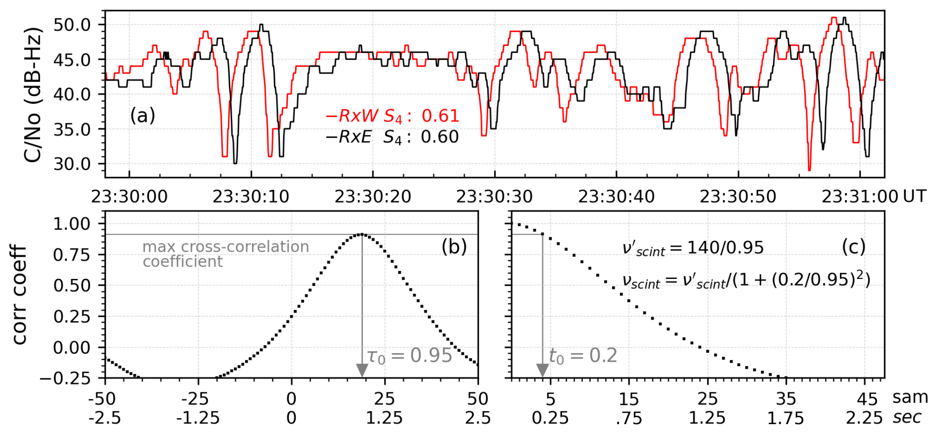
Figure 2 Illustration of the calculation used to derive the characteristic time (t₀) and the time lag of maximum correlation (τ₀). Panel (a) shows an example of 60 s signal strength measurements made with closely spaced ScintPi 3.0 monitors on 4 October 2022. Panel (b) shows the cross-correlation function between power series from the two receivers. Panel (c) shows the autocorrelation for the west receiver. The maximum cross-correlation coefficient is used to estimate the characteristic time associated with the signal decorrelation. The horizontal axes in panels (b) and (c) show both the sample number (sam) and time in seconds.

Further considerations

While most studies (e.g., Kil et al., 2000; Otsuka et al., 2006; de Paula et al., 2010) have used the Briggs formulation (Eq. 1), Ledvina et al. (2004) presented further analysis of the spaced-receiver technique and pointed out additional considerations. First, they highlighted the fact that the scintillation pattern velocity is a projected representation of the velocity of the irregularities, and this velocity will depend, in general, on geometric factors involving the placement of the receivers and the Earth's magnetic field. For instance, differences in the altitudes of the two receivers should be taken into consideration in the estimation of the drifts. They showed that Eq. (1) can be updated to account for differences in the heights of the receivers (Ledvina et al., 2004):

$$\begin{array}{}\text{(4)}& {\mathit{\nu }}_{\mathrm{scintx}}=\left[\mathrm{1}-{\displaystyle \frac{\mathrm{\Delta }h}{d}}\tan \left({\mathit{\theta }}_{\mathrm{vz}}\right)\right]\left[{\displaystyle \frac{v_{\mathrm{scintx}}^{\prime }}{\mathrm{1}+t_{\mathrm{0}}^{\mathrm{2}}/{\mathit{\tau }}_{\mathrm{0}}^{\mathrm{2}}}}\right],\end{array}$$

where ν_scintx represents the scintillation pattern velocity in the east–west direction parallel to the Earth's surface, d is the zonal spacing of the receivers, Δh is the height difference in the receivers and θ_vz is a projection angle in the vertical zonal plane. The projection angle is given by the following (Ledvina et al., 2004):

$$\begin{array}{}\text{(5)}& {\mathit{\theta }}_{\mathrm{vz}}={\tan }^{-\mathrm{1}}\left[{\displaystyle \frac{\tan \left(\mathit{\varphi }\right)\sin \left(\mathit{\theta }\right)-\left(B_x/B_y\right)\tan \left(\mathit{\varphi }\right)\cos \left(\mathit{\theta }\right)}{\mathrm{1}-\left(B_z/B_y\right)\tan \left(\mathit{\varphi }\right)\cos \left(\mathit{\theta }\right)}}\right],\end{array}$$

where ϕ is the satellite zenith angle and θ is the satellite azimuth angle relative to the magnetic meridian (magnetic north). B_x, B_y and B_z are components of the geomagnetic field vector at the IPP location in the magnetic east, north and vertical directions, respectively. B_x is close to zero and the second term in the tan ⁻¹ argument is negligible. The IPP was computed using a mean ionospheric altitude of 450 km that is thought to be adequate for the location and solar flux conditions of the observations (e.g., Nava et al., 2007). Perhaps more importantly, different choices of ionospheric altitude (e.g., 300–600 km) produce similar values of geomagnetic components and do not affect our drift estimates or results.

Using long-term averages of the GNSS coordinates provided by the receivers, we found a height difference of ∼ 15 m (Fig. 1c). Considering values for the experiment at UFCG (described in Sect. 2.2), the expression for the irregularity drifts using the geostationary measurements is updated to the following:

$$\begin{array}{}\text{(6)}& \begin{array}{rl}& {\mathit{\nu }}_{\mathrm{scintx}}\\ & =\left(\mathrm{1}-{\displaystyle \frac{\mathrm{15.3}}{\mathrm{140}}}\left[{\displaystyle \frac{\tan \left(\mathrm{48}\right)\sin \left(\mathrm{84}-(-\mathrm{21.39})\right)}{\mathrm{1}-\left(\frac{B_z}{B_y}\right)\tan \left(\mathrm{48}\right)\cos \left(\mathrm{84}-(-\mathrm{21.39})\right)}}\right]\right)\\ & \left[{\displaystyle \frac{v_{\mathrm{scintx}}^{\prime }}{\mathrm{1}+t_{\mathrm{0}}^{\mathrm{2}}/{\mathit{\tau }}_{\mathrm{0}}^{\mathrm{2}}}}\right]=\left(\mathrm{0.899}\right)\left[{\displaystyle \frac{v_{\mathrm{scintx}}^{\prime }}{\mathrm{1}+t_{\mathrm{0}}^{\mathrm{2}}/{\mathit{\tau }}_{\mathrm{0}}^{\mathrm{2}}}}\right].\end{array}\end{array}$$

Ledvina et al. (2004) also pointed out that deriving zonal irregularities' drifts from the scintillation pattern velocity can be affected by vertical ionospheric drifts (ν_iz) at the IPP location. The vertical drifts would affect the scintillation pattern velocity as follows:

$$\begin{array}{}\text{(7)}& v_{\mathrm{scintx}}=v_{\mathrm{zonal}}+\left[{\displaystyle \frac{-\tan \left(\mathit{\varphi }\right)\sin \left(\mathit{\theta }\right)}{\mathrm{1}-\left(B_z/B_y\right)\tan \left(\mathit{\varphi }\right)\cos \left(\mathit{\theta }\right)}}\right]{\mathit{\nu }}_{\mathrm{iz}},\end{array}$$

where $(B_z/B_y)$ is equivalent to the tangent of the inclination angle of the geomagnetic field (−(tan (ϑ_dip)) at the IPP location and v_iz is the vertical irregularity drift.

For our experimental setup, ϕ = 48°, θ = (105.39°) and ϑ_dip = −29.62°, resulting in ν_scintx = ν_zonal−0.917ν_iz. Here, the azimuth refers to the geographic azimuth of the satellite relative to the magnetic meridian. This means that, for our experimental configuration, the vertical drifts in conjunction with the geometry of the signal path can contribute to the magnitude of the observed scintillation pattern velocities. Outside the pre-reversal enhancement (PRE) time that occurs around sunset, vertical drifts are expected to be much smaller than the values of zonal drifts. Following previous studies (e.g., Cesaroni et al., 2021), the effect of the vertical drifts is not corrected for in our analyses.

4 Results and discussion

4.1 On the estimation of irregularity drifts

We now present and discuss the measurements made by the UFCG ScintPi monitors and the zonal irregularity drifts derived from these measurements. Figure 3 shows a representative example of the measurements and results. The measurements are for the night between 4 and 5 October 2022.

Figure 3 Example of measurements and analyses made with closely spaced ScintPi 3.0 monitors at UFCG for the same night as that shown in Fig. 2 (4–5 October 2022). Panel (a) presents the signal strengths (C$/$No; in dB-Hz) for L1 values from PRN136. Panel (b) displays the severity of scintillation, i.e., the S₄ index. Panel (c) shows the maximum value of the normalized cross-correlation function $\left|r\right|$. Only patterns for which $\left|r\right|$ > 0.5 (highlighted) are used in the computation of the scintillation pattern velocity in this study. Panel (d) shows the estimated mean characteristic velocities, whereas panel (e) presents the estimated mean true scintillation pattern velocities. Error bars in panels (d) and (e) represent the standard deviation around the mean of the values used in the 3 min bins.

Figure 3a shows L1 C$/$No values for the PRN136 signal measured by the two receivers. It shows that, as expected, similar variations in scintillation occurrence and magnitude were observed in both signals. Figure 3b shows 1 min S₄ index values computed for both signals. The S₄ index is a widely index used in scintillation studies to quantify amplitude scintillation (Groves et al., 1997; Kil et al., 2002; Nishioka et al., 2011) and can be defined as the standard deviation of the signal intensity normalized by its average. The observed S₄ values indicate (i) strong L-band scintillation occurring from 22:30 to 23:45 UT (20:30 to 21:45 LT) and (ii) moderate–weak scintillation between 00:30 and 02:30 UT (22:30 and 00:30 LT). Note that the estimates of S₄ for both signals provide nearly identical values most of the time, indicating similar variability in the intensity patterns. This similarity in the signals is better quantified in the high cross-correlation coefficients (i.e., $\left|r\right|$ ≥ 0.75) presented in Fig. 3c.

Figure 3c also shows that, despite the reduced resolution of the signal intensities, high correlation values can still be derived from ScintPi measurements. Additionally, we point out that high cross-correlation coefficients persisted even during weak scintillation activity (i.e., S₄ in the 0.2–0.4 range), indicating that one can compute irregularity drifts even during periods of weak L-band scintillation.

Figure 3d presents the estimates of the characteristic velocity (ν_c). The characteristic velocity has been averaged in 3 min bins (average of three values). The error bars represent the standard deviation of the values used in the averages. One can observe that the characteristic velocity shows higher values early in the evening. We attribute this to periods of more turbulent irregularity motion associated with the development of EPBs. This turbulent or random behavior has been observed in previous studies (e.g., Spatz et al., 1988; Bhattacharyya et al., 2001; Valladares et al., 2002; Kintner et al., 2004; Otsuka et al., 2006).

Finally, Fig. 3e shows our estimates (3 min averages) of the corrected true scintillation pattern velocities (v_scintx). Again, error bars represent the standard deviation of the values used in the averages. As expected, the scintillation pattern velocities reveal a behavior that is similar to that expected for the low-latitude drifts. They show strong eastward drifts early in the evening with weakening drifts towards midnight.

4.2 On the seasonal variability in zonal irregularity drifts

The analysis described in Sect. 4.1 was applied to a dataset containing 242 observation nights between 1 September 2022 and 30 April 2023. The period covers the equatorial spread F (ESF) season in Brazil (Abdu et al., 2003), when scintillation is observed. This period also has measurements from two equinoxes and the December solstice. The results are summarized in Fig. 4.

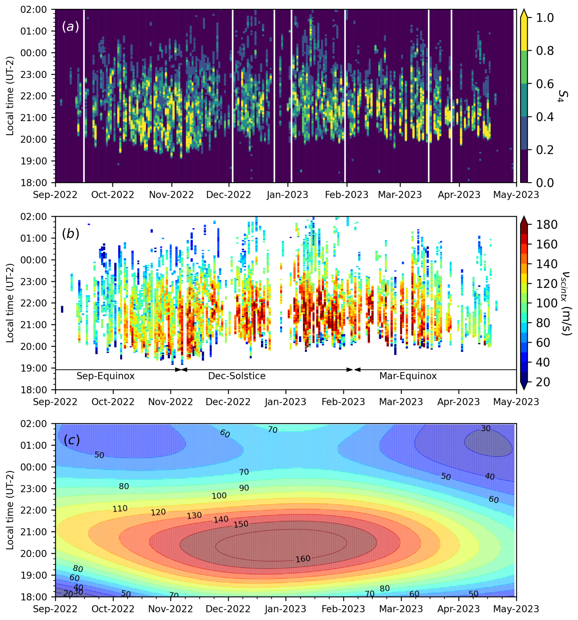
Figure 4 Panel (a) shows the average S₄ index measurements as a function of local time (LT = UT−2) and date for 242 nights between 1 September 2022 and 30 April 2023. The average is for the two S₄ values computed by the spaced monitors. White lines indicate a lack of data caused by power outages at the observation sites. Panel (b) shows zonal irregularity drifts. Different seasons, determined as ±45 d around equinox and solstice days, are also indicated. Panel (c) shows climatological zonal wind velocities (U_z) from the Horizontal Wind Model 14 (HWM14) for a height of 450 km over UFCG; its magnitude values are indicated by the contour line labels.

Figure 4a shows the variation in the observed L-band (1.575 GHz) scintillation as a function of local time and day of the campaign. The vertical white lines indicate missing data due to power outages at at least one of the receiver sites. Figure 4a also displays the day-to-day variability in the scintillation activity observed by the monitors. Moreover, it shows that scintillation occurred on most days. Further, Fig. 4a shows that L-band scintillation was mostly observed between 20:00 LT and local midnight. During some days, however, scintillation occurred until 02:00 LT.

Figure 4b summarizes the magnetic zonal irregularity drift results. The drifts show a behavior that indeed is similar to what would be expected for background nighttime ionospheric plasma drifts at low latitudes (Fejer et al., 1991, 2005). The drifts are predominantly eastward, with larger values (120–200 m s⁻¹) during the early evening, gradually decreasing to 20–80 m s⁻¹ by midnight and into the post-midnight sector. The results in Fig. 4c also show a trend, with lower drift values in September–October and April–May and higher values in the months between.

As mentioned earlier, zonal irregularity drifts are often assumed to be tracers of ionospheric plasma drifts (Ledvina et al., 2004). At low latitudes, theoretical analyses suggest that nighttime zonal drifts are expected to be controlled, in most part, by zonal F-region winds (Rishbeth, 1972; Heelis et al., 1974). For instance, zonal plasma drifts are related to zonal neutral winds (U_z) through a flux-tube-integrated Pedersen-conductivity-weighted integral which is representative of the neutral wind dynamo (Haerendel et al., 1992):

$$\begin{array}{}\text{(8)}& {\mathit{\nu }}_{\mathrm{zonal}}\sim {\displaystyle \frac{\mathrm{1}}{{\mathrm{\Sigma }}_{\mathrm{P}}}}\int {\mathit{\sigma }}_p{U}_{\mathrm{z}}\mathrm{d}s,\end{array}$$

where the integral is performed along a magnetic field line, σ_p is the Pedersen conductivity and Σ_P is the Pedersen conductance. At night, E-region conductivities are greatly reduced and zonal drifts are expected to have contributions coming, predominantly, from winds at F-region heights.

Figure 4c shows the magnetic zonal component of the neutral winds at F-region heights (450 km) over UFCG predicted by the Horizontal Wind Model 14 (HWM14). HWM14 is an empirical model of the neutral winds developed using an extensive set of measurements (Drob et al., 2015). It provides estimates of the geomagnetic quiet-time behavior of the thermospheric winds. Similar to the observed behavior of the irregularity drifts, Fig. 4c shows stronger eastward winds in the early evening and weaker winds towards midnight and into the post-midnight sector. Additionally, HWM14 results show weaker zonal winds in September–October and April–May, contrasting with stronger zonal winds in the months between November and March. The similarity in the behavior between drifts and winds is impressive, given that the plasma drifts depend on combined contributions of winds along magnetic fields, weighted by the conductivity values. We must point out that similarities in the behavior of EPBs and neutral wind magnetic zonal velocities have been reported out before using, for instance, same-night observations made by airglow cameras and Fabry–Pérot interferometers (FPI) located near our site (UFCG) in Brazil (Chapagain et al., 2012).

We point out that the magnitudes of the winds and irregularity drifts differ, with irregularity drifts being, in general, larger than the zonal winds. The difference is attributed to the fact the drifts are the result of conductivity-weighted winds along the magnetic field lines (Eq. 5), whereas the HWM14 winds shown here are for a single height and location (450 km above UFCG). Observations of neutral winds larger than ionospheric drifts have been reported in previous studies (e.g., Wharton et al., 1984; Coley et al., 1994; Navarro and Fejer, 2020). Additionally, HWM14 does not have a solar flux dependency and is representative of the solar conditions under which the drift measurements were made.

Finally, we also point out cases of very low irregularity drift values early in the evening on certain observation nights. See, for instance, the blue markers in some of the drift measurements between 19:00 and 20:30 LT in Fig. 4b. We hypothesize that these low values of zonal drifts can be caused by the contribution of large vertical drifts, associated with the PRE, to the estimates of zonal drifts (Eq. 7). Estimates of nighttime vertical drifts derived from digisonde data for a low-latitude site in Brazil have revealed cases of upward drifts as large as 40 m s⁻¹ during the same time frame of 19:00 and 20:30 LT (e.g., Abdu et al., 2006).

5 Conclusions

We presented the results of an experiment to evaluate the use of ScintPi 3.0 to estimate ionospheric irregularity drifts. ScintPi 3.0 is an alternative, low-cost, GNSS-based scintillation monitor developed to enable research, education and citizen science initiatives (Gomez Socola and Rodrigues, 2022). Of relevance to this study is that ScintPi 3.0 is capable of measuring signals transmitted by geostationary satellites.

The experiment used the spaced-receiver scintillation technique for measurements of ionospheric irregularity drifts (Briggs et al., 1950; Ledvina et al., 2004). It also used measurements made by two ScintPi 3.0 deployed in Campina Grande, Brazil (7.21° S, 35.91° W; dip latitude ∼ 14° S). The monitors were spaced at a 140 m distance in the magnetic east–west direction to measure the zonal component of the drifts associated with scintillation-causing equatorial spread F (ESF) irregularities.

We analyzed measurements made throughout an entire ESF season, between September 2022 and April 2023. We focused our analyses on irregularity drifts derived from geostationary satellite signals, which simplified the analyses and interpretation of the results.

The results confirm that ScintPi 3.0, despite its low cost and low C$/$No resolution (1 dB-Hz), can measure irregularity drifts. The cross-correlation of the signals is mostly well above 0.75, even during late-night weak scintillation. Our drift calculation results also show that the local time variation in the estimated irregularity zonal drifts is in good agreement with previous experimental studies and with theoretical expectations for the behavior of the low-latitude background zonal plasma drifts (e.g., Haerendel et al., 1992; Fejer et al., 2005; Shidler and Rodrigues, 2021). The drifts are predominantly eastward, with the largest values early in the evening and weakening drifts towards local midnight.

Our results also reveal a seasonal trend in the irregularity zonal drifts. We found that this trend is well correlated with the behavior of the zonal component of the thermospheric neutral winds, as predicted by the HMW14. The similarity between the behavior of the neutral winds and observed irregularity drifts is a manifestation of the F-region dynamo, which controls the zonal F-region drifts at night (e.g., Haerendel et al., 1992).