Accurate humidity probe for persistent aviation-contrail conditions

We present a state-of-the-art humidity probe for in situ airborne water vapor measurements tailored to the humidity range relevant for the formation of persistent aviation contrail cirrus clouds. Our probe is based on tunable infrared laser direct absorption spectroscopy (TILDAS). We scan a laser in wavelength across an isolated water (H₂O) absorption line at 7205.246 cm⁻¹ (1.39 µm) to obtain the H₂O volume mixing ratio in sample air at 1 Hz in real time. Our optical design features a combination of single-mode optical fibers and a short-path absorption cell with integrated focusing optics and detector to avoid any absorption path outside of the sample volume. A parallel fiber path and detector capture the laser power profile during the wavelength scan for spectral-baseline normalization. We have built and tested two prototypes and tested them side-by-side in the laboratory against a humidity standard as well as against each other. Without any calibration, we found agreement against the humidity standard of better than 98 % for the relevant H₂O range below 200 ppm. The agreement between both instruments when operated in series measuring the same sample air was 99.7 %. The stability of both instruments was quantified to be ±1 % (1σ) during a 5 d long period where both prototypes operated without any temperature control. We show that our probes can measure H₂O with linear response over 4 orders of magnitude.

1 Introduction

Persistent aviation contrail cirrus clouds are increasingly recognized as a dominant contributor to the non-CO₂ climate impacts of aviation (Kärcher, 2018; Quaas et al., 2021; Voigt et al., 2021; Spangenberg et al., 2013). These clouds form when water vapor from aircraft exhaust condenses and freezes in the cold upper troposphere, particularly under ice-supersaturated conditions. If ambient atmospheric conditions are favorable, such as sufficiently low temperatures and high humidity with respect to ice (RH_i), these contrails can persist and evolve into extensive cirrus cloud fields, contributing significantly to the Earth's radiative budget through their ability to trap outgoing longwave radiation (Lee et al., 2021; Bock and Burkhardt, 2016).

The effective radiative forcing (ERF) from contrail cirrus is now estimated to exceed that of aviation CO₂ emissions over the same time period. According to the updated assessment by Lee et al. (2021), the ERF of contrail cirrus is approximately 57.4 mW m⁻², compared to 34.3 mW m⁻² from aviation-induced CO₂, highlighting their substantial contribution to aviation's climate impact. Consequently, the need for accurate understanding and mitigation of contrail cirrus has become increasingly urgent.

A central factor in the formation and persistence of contrail cirrus is atmospheric humidity (Appleman, 1953). Specifically, the local relative humidity with respect to ice (RH_i) determines whether the ambient conditions support contrail formation and whether these ice crystals will sublimate or persist (Schumann, 1996; Minnis et al., 2004). Slightly subsaturated or supersaturated air with respect to ice is a prerequisite for persistent contrails (Li et al., 2023). Small variations in humidity at cruising altitudes dramatically affect their lifecycle by controlling ice crystal formation, growth and dissipation (Unterstrasser and Gierens, 2010). Therefore, highly spatially and temporally resolved humidity measurements are essential for accurate modelling and prediction.

Approximate H₂O concentration thresholds for RH_i >100 % at various altitudes may be calculated using the standard atmosphere model (ISO 2533:1975; International Organization for Standardization, 1975). For example, at an altitude of 9 km (p∼307 hPa, T∼230 K) the standard atmosphere presents RH_i >100 % at H₂O >279.5 ppmv. At 12 km altitude (p∼193 hPa, T∼217 K) H₂O >89 ppmv satisfies RH_i >100 %. In the real upper troposphere, H₂O as low as 30 ppmv may frequently be observed at cruise altitudes in cloudy conditions, with a sharp drop in probability below this humidity. The upper limit in cloudy conditions at cruise altitude may be placed at 150 ppmv, though the probability distribution has a wider tail towards higher humidity (Dyroff et al., 2015).

In situ measurements of atmospheric humidity and temperature have proven critical to improving our understanding of contrail microphysics and their radiative effects. Campaigns such as MOZAIC/IAGOS (Marenco et al., 1998; Petzold et al., 2015) and CARIBIC (Brenninkmeijer et al., 2007) have provided large-scale, long-term observational datasets using commercial aircraft platforms, allowing the evaluation of supersaturated regions and the frequency of contrail formation (Gierens et al., 2020; Petzold et al., 2020; Li et al., 2023). These datasets are also foundational to the development of contrail-avoidance strategies, where flight trajectories are dynamically adjusted to avoid regions with high RH_i (Teoh et al., 2022). The application of such strategies in flight planning has shown promising results in simulations, with the potential to reduce contrail-related climate forcing significantly (Matthes et al., 2020).

Research-grade airborne humidity sensors have been demonstrated and further enhanced the capability of the scientific community. These include frost-point hygrometers (Hall et al., 2016; Vömel et al., 2016), Lyman-α fluorescence sensors (Meyer et al., 2015; Sitnikov et al., 2007), mass spectrometers (Kaufmann et al., 2016), and tunable diode laser absorption spectrometers (Zondlo et al., 2010; Dyroff et al., 2015; Buchholz et al., 2017; Buchholz and Ebert, 2018; Sarkozy et al., 2020; Graf et al., 2021). These instruments have been used for precise water vapor measurements, but they are one-off instruments for dedicated research campaigns.

The only commercially available and/or flight certified instruments are the WVSS-II (Vance at al., 2015) formerly offered by Spectra Sensors and now by FLYHT (https://flyht.com/weather-sensors/wvss-ii/, last access: 6 January 2026), and the IAGOS core humidity (ICH) sensor (Helten et al., 1998, see also https://www.iagos.org/iagos-core-instruments/h2o/, last access: 6 January 2026) developed by Forschungszentrum Jülich GmbH in cooperation with enviscope GmbH and is manufactured by enviscope GmbH under licence agreement. WVSS-II is a laser-based sensor developed for higher humidity. While offering fast response, its stated detection limit of 50 ppmv and absolute uncertainty of ±50 ppmv or ±5 % (whichever greater) (Vance et al., 2015; Williams et al., 2021; Kaufmann et al., 2018; Groß et al., 2014) it is less suited for the contrail-cirrus relevant humidity range of as low as 30 ppmv, but it remains a powerful tool for lower and middle troposphere measurements.

The ICH instrument measures humidity using a capacitive relative humidity sensor. The sensor technology is very mature, and it is also used on radiosondes to measure vertical profiles of humidity from weather balloons. Its limitation is a very slow time response at low absolute humidity on the order of 2 min (Neis et al., 2015). During this time a jet aircraft at cruising altitude would travel around 30 km. Laser-based systems can provide resolution of 1 km or better.

Many of the above-mentioned instruments have been compared to reference instruments in airborne or laboratory settings. Brunamonti et al. (2025) report agreement of various instruments to within ±7 % at H₂O >10 ppmv during the AquaVIT-4 campaign at the AIDA cloud chamber. This level of agreement under controlled test conditions is very impressive.

Here we describe a new laser-based humidity probe specifically designed for, but not limited to, measurements of upper-tropospheric humidity levels relevant to aviation contrail cirrus. Our design is simple and robust with cost-efficient and scalable production in mind. Our system overcomes the limitations of currently available commercial instruments in terms of sensitivity and time response. In this paper we demonstrate the performance of two prototypes in a laboratory setting.

2 Instrument design

2.1 Optics

Our humidity probe is based on direct laser absorption spectroscopy using an all-fiber based optical system. We use a fiber-coupled distributed feedback (DFB) diode laser (AERODIODE, France) to probe an isolated absorption line of H₂O at a wavelength of 1.39 µm (7205.246 cm⁻¹). We chose this wavelength because we were able to use fiber-coupled lasers originally designed for optical telecommunication (E-band). This technology is very mature, and lasers as well as fiber-optical components and detectors are readily available at relatively low cost. We use a 50:50 fiber-based beam splitter (Thorlabs, TW1430R5A1) to produce two fiber paths of similar optical power from the primary fiber; the sample path and the baseline path (see Fig. 1). For the sample path we use a single-mode fiber pigtail with glass ferrule termination (Thorlabs, SMPF0115-APC). We use a graded-index (GRIN) lens (Thorlabs, GRIN2313A) to create a slightly focused laser beam.

In a first step, a stainless-steel GRIN lens holder is mounted in a production jig that mimics the sample cell geometry while allowing good access to the GRIN lens and fiber ferrule. Both the fiber ferrule and the GRIN lens are permanently glued to the holder using UV-curing adhesive (Thorlabs, NOA61). The small gap between the ferrule and the GRIN lens is bridged with the same glue, which is transparent at the working wavelength and has a similar refractive index to the fiber ferrule and GRIN lens. Before curing the adhesive, the laser beam is aligned on the optical axis with the GRIN lens held in a 3-axis translation stage. The beam is aligned through a pinhole target onto a detector at 30 cm distance from the GRIN lens. Both the pinhole and the detector are located precisely centered on the optical axis. Once alignment is achieved, the glue is immediately cured using ultraviolet (UV) light and GRIN lens holder assembly can be transferred to the sample cell.

The GRIN lens holder has a tapered locating feature, and the sample cell has an equivalent tapered bore, similar to tapered tool holders, e.g. in a milling machine. This allows the GRIN lens holder to be placed centered on the cell's optical axis without any optical adjusters after transferring it from the alignment jig. An O-ring on the tapered face creates a vacuum seal and allows replacement of the GRIN lens assembly should it be required.

The opposite side of the stainless-steel sample cell body holds the sample detector (Thorlabs, PDAPC4). The detector is also integrated into the sample cell. To do so, we first bond an anti-reflection coated wedged window (Thorlabs, PS814-C) to the angled (1°) end face of the cell using NOA61. This window forms the gas seal of our single-pass sample cell with around 30 cm pathlength and internal volume of 72 cm³. We then align and bond the sample detector onto the outward face of the wedged window using NOA61. The position is defined by two 3D-printed detector holders (not shown in Fig. 2). The cell face and wedge angles are chosen such that all reflections from the intermediate surfaces are reflected away from the optical axis or do not re-enter the sample cell entirely. This effectively eliminates optical interference within the sample cell, which could otherwise cause temperature-driven instrument drift. The sample cell has two gas ports for the sample gas in and out flow. A thermistor (YSI 44032, 30 kΩ at 25 °C) is threaded into the stainless-steel cell body near the cell center.

The cell design with the GRIN lens holder and the integrated sample detector effectively eliminates all optical pathlength outside of the sample cell that could otherwise be subject to generating absorption signal not due to the sample volume. Furthermore, the sealed laser package and the sealed detector package are back-filled with H₂O-free air or nitrogen as specified by the manufacturers. This is very important for our humidity probe, as the sample will often contain humidity two orders of magnitude lower than the air surrounding the probe, e.g. an aircraft cabin. We thus eliminate any unknown zero offset in our humidity measurements.

The second fiber path created by the fiber Y-splitter is connected to a single-mode fiber pigtail with glass ferrule termination (Thorlabs, SMPF0115-APC). The glass ferrule is directly bonded to the window of the baseline detector (Thorlabs, PDAPC4). We use this detector to measure the optical power profile of the laser diode as it is scanned in wavelength via injection current. The resulting baseline spectrum does not contain any signal due to absorption of H₂O. We are using this baseline spectrum to continuously normalize the sample spectrum in our spectroscopic fit model.

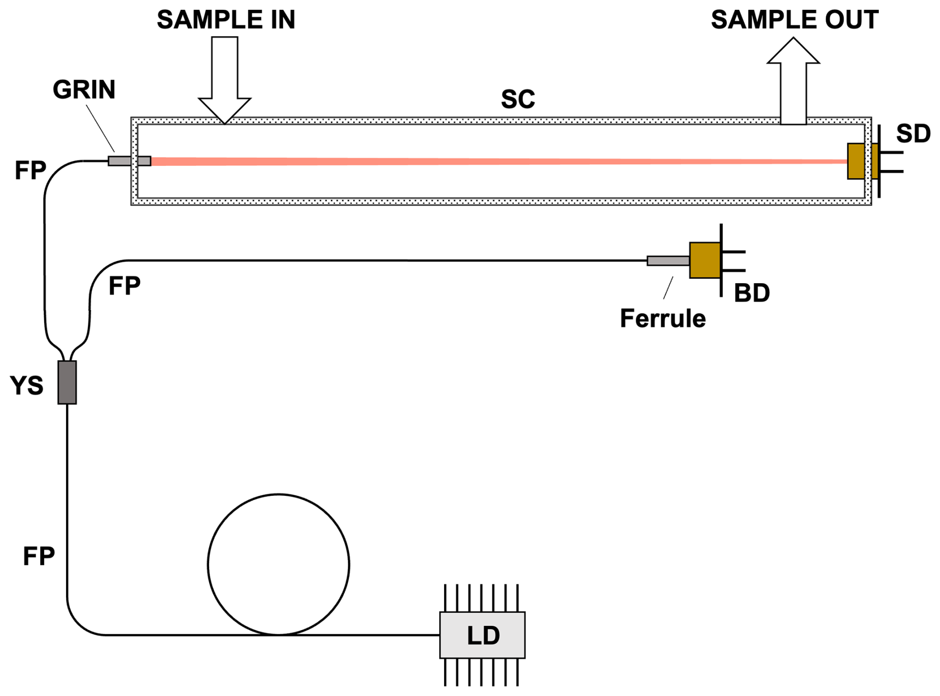
Figure 1 Schematic of the humidity probe. LD: laser diode; FP: fiber pigtail; YS: fiber Y-splitter; SC: sample cell; SD: sample detector; BD: baseline detector.

Figure 2 CAD rendering of the sample cell. Not all components shown. GRIN lens holder not in final position. 1: fiber pigtail; 2: GRIN lens; 3: stainless-steel cell body; 4: thermistor location; 5: wedged window; 6: detector; 7: gas ports. The optical pathlength is around 30 cm and the cell volume is 72 cm³.

2.2 Electronics

Two prototypes were built and tested with the same optical system, but with different electronics packages. For prototype 1 we used a data acquisition system equivalent to what we use in the larger commercial Aerodyne Research TILDAS instruments. This technology is very mature, offers the lowest possible noise, and it served as our benchmark during this study. A personal computer (PC) operated the in-house TDLWintel software package. The software communicated with a set of National Instruments (NI) data acquisition cards. The laser was driven using a state-of-the-art laser driver (Wavelength Electronics QCL-125) with very low current noise. Upon pre-averaging of the spectra, they were fit in TDLWintel at 1 Hz in real time to produce H₂O mixing ratios using the measured sample-gas temperature and pressure.

For prototype 2 we used a different electronics system (RedWave Labs, Universal Platform for Spectroscopic Instruments). This technology was obtained for this project due to its very compact design and integration of up to 3 low-noise laser drivers. While similar in principle to the prototype 1 system, it combines a low power PC, up to 3 laser drivers, and a data acquisition system into a very compact unit. We have developed software that operates the Universal platform with one laser. Spectra were pre-averaged on the unit's field programmable gate array (FPGA) before being transferred to the PC for processing and storage. The lasers and detectors of both prototypes are the same model and vendor.

2.3 Spectroscopy

The laser wavelength was rapidly scanned by linearly ramping the laser injection current in time from below threshold to 50 mA (70 mA for prototype 2) at a frequency of 2666 Hz (334 Hz for prototype 2) as shown in Fig. 3. The final 10 % of the time of each laser scan, the laser was operated below threshold to record the detector dark signal. The scan frequency was a consequence of the data-acquisition system clock (prototype 1: 1333 kHz; prototype 2: 588 kHz) and the number of points per spectrum scan (prototype 1: 500; prototype 2: 880) as well as whether one or two detector signals were acquired simultaneously (prototype 1: 1; prototype 2: 2). At the time of the experiments, the prototype 2 system clock of 588 kHz was the fastest data rate our software was supporting. The RedWave system hardware supports a clock frequency of up to 2 MHz. The 2666 spectra (334 spectra prototype 2) were continuously digitized and combined to a one-second average spectrum before being transferred to the PC. For prototype 1 the sample and baseline spectra were recorded interleaved. Every minute, 50 s of 1 Hz sample spectra were followed by one 10 s average baseline spectrum. To record both spectra with only one analog-to-digital (ADC) converter available we used a signal multiplexer to switch between the sample and baseline detector. For prototype 2 we were able to acquire both sample and baseline detector signals simultaneously using two ADCs at the cost of a lower number of spectra averaged in 1 s. With prototype 2 we recorded spectra on the device and then fit them offline using the same fitting engine as embedded in TDLWintel, though the fit setup was adjusted for the different laser and its scan. In both systems, the wavelength scale is projected on the time base of the instrument by a laser-dependent non-linear tuning rate function (Fig. 3 lower panel). This function was empirically measured for each laser using the resonant fringe pattern of a 25 cm long glass rod (Edmund Optics, Stock #84-531) with uncoated plane-parallel end faces that served as etalon. The maxima and minima of the fringe pattern are equally spaced in wavelength, and we were thus able to infer the relative wavelength tuning of the laser, while the H₂O transition wavelength obtained from the HITRAN database (Gordon et al., 2017) provided the anchor point in the spectrum for the absolute wavelength scale.

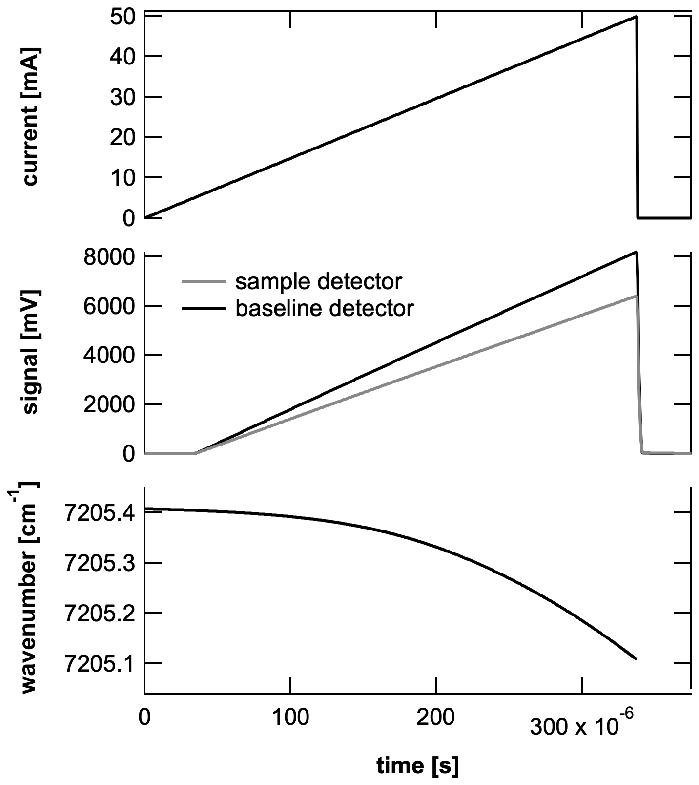
Figure 3 Laser scan parameters for prototype 1. The prototype 2 laser was scanned slower due to a different hardware configuration. For the low H₂O concentrations discussed here, the H₂O absorption feature cannot be resolved by eye in the sample detector spectrum (grey trace). For a transmission spectrum see Fig. 4.

Figure 4 shows the transmission spectrum of H₂O recorded at 1 Hz by prototype 1 at three different concentrations: 6.5, 13, and 26 ppm. The grey dots are the measured baseline-normalized spectra, and the black lines are the fit. The signal (fractional absorption line depth) and fractional absorption noise in the baseline are quantified and given in the figure. For the fit we first perform a zero-offset correction of each 1 s spectrum and the baseline spectrum using the detector signals during the laser-off period at the end of the scan. We then divide the sample spectrum by the baseline spectrum and normalize the resulting spectrum to transmission space (0 to 1). Last, we perform a non-linear least squares fit of the normalized spectrum to a calculated spectrum based on the Beer-Lambert law, HITRAN database parameters for the considered absorption lines, and the instantaneous sample temperature and pressure measurements. This fit includes a composite spectrum of 14 H₂O lines between 7204 and 7206 cm⁻¹ of which the main line probed (7205.246 cm⁻¹, see Table 1) has a linestrength at least 50× higher than all other lines in this wavenumber window. We used a Voigt lineshape model to describe the absorption lines, and we did not include self-broadening of the H₂O lines. A third-order polynomial captures any residual baseline curvature that arises from slightly different response of the sample and baseline detectors.

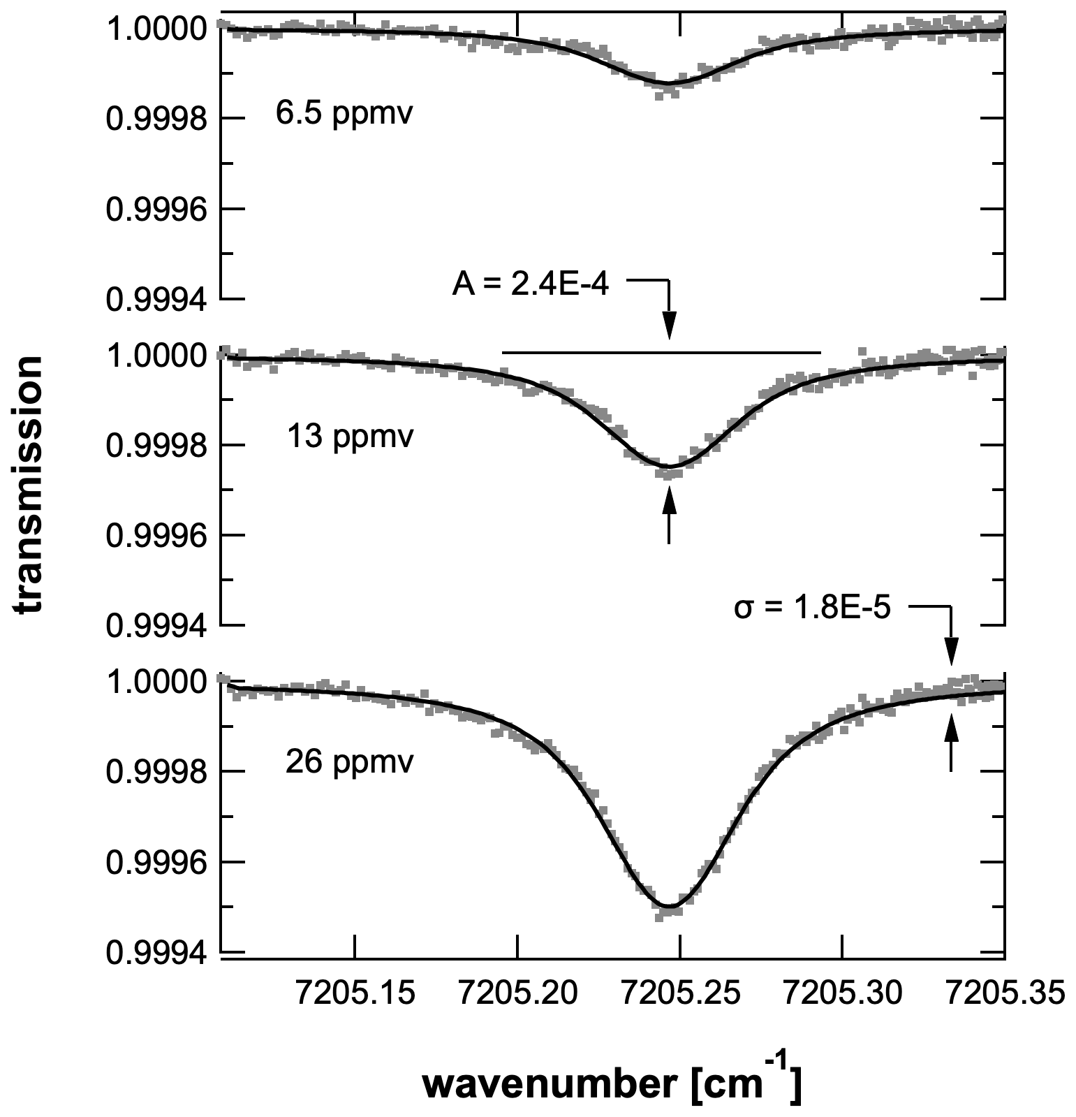
Figure 4 Measured 1 s average transmission spectra of H₂O at different concentrations. The grey dots are the measurement, and the black lines are the fit. Absorption signal A and the noise σ in the spectral baseline are given.

Table 1 Spectroscopic parameters we used as basis for the spectral line fit. The parameters were retrieved from the HITRAN2016 database. ID: molecule/isotopologue ID; ν₀: line-center wavenumber; S_ij: integrated linestrength; γ_air: air-broadening coefficient; E^′′: ground-state energy; $\mathrm{d}{S}_{ij}/\mathrm{d}T$: temperature coefficient of S_ij. The parameter uncertainty is given in brackets where available. The temperature coefficient of the linestrength of this line is −0.004 K⁻¹.

3 Instrument characterizations

3.1 Test setup

For the performance evaluation of our prototype instruments, we have set up the humidity-generation system shown in Fig. 5. We used a flow of around 1.5 standard liters per minute (slpm) of ultra-zero air (UZA) with H₂O <3 ppmv from a compressed cylinder as feedstock. The UZA was further dried by passing through a Nafion dryer followed by a trap filled with molecular sieve at room temperature. The flow through the sample cell (10) and the pressure of the sample gas (11) were set to 1 slpm and 213 hPa (160 Torr), respectively, using the two manual flow restrictors (5) and (12). A pump (13) generated the required vacuum downstream of the sample cell. The remaining UZA flow was discarded via an overblow port (4).

We used a dew-point generator (6, Licor LI-610) to generate a flow of around 1.5 slpm of saturated humid air set manually by a flow restrictor (7). Of this flow, a small flow of 0 to 10 standard cubic centimeters per minute (sccm) could be directed into the low-pressure UZA flow via a flow controller (9). The remaining flow was discarded via an overblow port (8). With this system we were able to generate a gas flow with humidity ranging from (near) zero parts per million by volume (ppmv) to around 125 ppmv.

The bubbler of the DPG was exposed to ambient pressure, which was changing with the local weather pattern. This resulted in variations of the saturated absolute humidity generated by the DPG (relative humidity remained at 100 %). To this end we have calculated the expected absolute humidity provided by the DPG taking the ambient pressure into account. We used the Buck formula to calculate the saturated H₂O partial pressure $p_{{\mathrm{H}}_{\mathrm{2}}\mathrm{O}}$ (in hPa) from the DPG based on the DPG temperature setpoint T (in °C):

$$\begin{array}{}\text{(1)}& p_{{\mathrm{H}}_{\mathrm{2}}\mathrm{O}}=\mathrm{6.1121}\cdot \exp \left({\displaystyle \frac{\mathrm{18.678}-T}{\mathrm{234.5}}}\cdot {\displaystyle \frac{T}{\mathrm{257.14}+T}}\right).\end{array}$$

We then calculated the generated H₂O in ppmv using the local atmospheric pressure p_atm (in hPa):

$$\begin{array}{}\text{(2)}& {\mathrm{H}}_{\mathrm{2}}\mathrm{O}={\displaystyle \frac{p_{{\mathrm{H}}_{\mathrm{2}}\mathrm{O}}}{p_{\mathrm{atm}}}}\cdot \mathrm{1}E\mathrm{6}.\end{array}$$

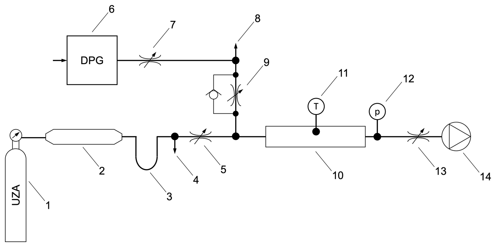
Figure 5 Schematic of our laboratory humidity-generation system. (1) UZA tank; (2) Nafion dryer; (3) desiccant trap; (4) overblow port; (5) flow restrictor; (6) dew-point generator; (7) flow restrictor; (8) overblow port; (9) flow controller; (10) sample cell; (11) thermistor; (12) pressure sensor; (13) flow restrictor; (14) vacuum pump.

The saturated humidity from the DPG set to T=10 °C was typically around 12 000 ppmv depending on the atmospheric pressure (Eqs. 1 and 2). With a dilution of up to 10 sccm into 1 slpm (100×) the maximum humidity of our generated humidified UZA was around 120 ppmv. The minimum humidity was assumed 0 ppmv, but it is possible that up to 1 ppmv remained after passing the UZA through the Nafion dryer and desiccant. With this setup, our laboratory testing was based around ramping the generated humidity between dry (nominally 0 ppmv) and around 120 ppmv. Each ramp contained 9 humidity levels with quasi-randomized order that lasted one hour in total. We remained at every humidity level for 5 min and at the final zero-air level for 20 min. An example time series is shown in Fig. 6.

Unfortunately, our DPG failed shortly after this measurement, and it remained the only hour of data where both prototypes measured the accurately generated humidity simultaneously. We show in a later section how well both prototypes agree with each other.

Figure 6 (left) Humidity ramp as described in text. We note that the flow controller at the highest setting likely did not provide the expected flow of 10 sccm and thus both prototypes reported lower humidity than expected as shown by difference of measurement to expectation (ΔH₂O). A double-exponential fit to the measurement suggests a response time of 2.8 s with a tail of 25 s due to desorption of H₂O from the cell and tuning walls. (right) Measured H₂O of both prototypes against the expected H₂O from the DPG system showing excellent linearity.

3.2 Response to humidity changes

We have determined the response time of our prototypes to changes in humidity using a double-exponential fit to the falling edge from 50 to 0 ppmv in Fig. 6. The two time constants were 2.8 and 25 s at the flow rate of 1 slpm and at room temperature. This is compared to a volumetric response of approximately 0.9 s considering the cell volume (72 cm³), flow rate (1 slpm), and sample pressure (213 hPa). The slightly slower response than the pure volumetric response is due to adsorption and desorption of H₂O on the cell and upstream-tubing walls and it is expected for the polar H₂O molecule. In our experiment we made no efforts to minimize the response time via faster flow or heating of the cell and tubing as we were focusing on quantifying the prototype accuracy. In future applications of our humidity probes, the flow rate will be higher and the cell and tubing will be heated to minimize adsorption and desorption effects and thus fasten the response. For context, in an airborne deployment onboard a commercial aircraft at cruise velocity of 250 m s⁻¹ this corresponds to a horizontal resolution of 700 m (fast time constant).

3.3 Noise

We have quantified the noise of both systems using the 1-second humidity data of both prototypes shown in Fig. 6. To this end we have calculated the Allan deviation (${\mathit{\sigma }}_{\mathrm{Allan}}=\sqrt{\frac{\mathrm{1}}{\mathrm{2}}{\left({{\mathrm{H}}_{\mathrm{2}}\mathrm{O}}_{i+\mathrm{1}}-{{\mathrm{H}}_{\mathrm{2}}\mathrm{O}}_i\right)}^{\mathrm{2}}}$) of the measured humidity of each of the 9 humidity levels, where ${{\mathrm{H}}_{\mathrm{2}}\mathrm{O}}_{i+\mathrm{1}}$ and ${{\mathrm{H}}_{\mathrm{2}}\mathrm{O}}_i$ are adjacent humidity measurements. We have neglected those measurements when the humidity was changed during the experiment as it would create a false high σ_Allan. The signal to noise is excellent with the 1 Hz noise around 0.1 ppmv in the contrail-relevant humidity range <200 ppmv as shown for both prototypes in Fig. 7. The slightly higher noise of prototype 2 is related to the slower scan rate.

Figure 7 Box plot of H₂O noise of both prototypes at 1 Hz measurement frequency defined as Allan deviation.

The low noise was achieved by using low-noise components. Both prototypes use very-low current-noise laser drivers that are among the best on the market. This ensures both low amplitude and wavelength noise, both of which contribute to mixing-ratio noise when fitting absorption spectra. The telecommunication lasers used have very low intensity noise. We furthermore chose low-noise detectors. In addition to the low-noise commercial components, prototype 1 uses a custom-designed low-noise power supply unit. Prototype 2 uses the built-in low-noise power supply unit of the RedWave data acquisition system. A more detailed discussion of the noise terms relevant in spectroscopy and a measurement of laser intensity noise of a similar telecommunication laser are given in Dyroff (2011).

3.4 Accuracy

We have quantified the accuracy of our humidity probe (prototype 1) by performing a 50 h long measurement of known humidity in a range of 0 ppmv to around 120 ppmv. The known humidity was delivered to the humidity probes by the humidity-generation system shown in Fig. 5. Each hour of the measurement consisted of 9 humidity levels, 8 levels of 5 min duration each followed by a 20 min period of zero air. The 1 s humidity measurements of each level were averaged for the last 4.5 min of each non-zero level to one average value per level. The final level was zero air, and it was measured for 20 min and averaged for 19.5 min. We then performed linear fits of the individual humidity ramps and derived the slope (measured vs. generated H₂O), zero offset, and r². The fit parameters were unconstrained. Figure 8 depicts the humidity time series in the top panel, followed by the slope, the zero offset, and r².

Figure 8 (top) Time series of a 50 h long measurement of prototype 1. Each hour was fit with a linear function, and the lower panels show the individual slopes, offsets, and goodness of fit (r²). The shaded areas of the slope panel show the uncertainty of the DPG humidity of ±1.3 % and the flow uncertainty of ±0.9 %.

On average we found an agreement of the prototype 1 instrument with the expected humidity from the DPG of 0.984±0.004 (slope in Fig. 8), i.e. the measured humidity was 1.6 % lower than expected. We also found that the zero air appeared to have around 1 to 2 ppmv of residual humidity, independently of our efforts to dry it further. See the prototype intercomparison below for evidence of this claim. In the future we consider using a liquid-nitrogen cold trap to freeze out the residual humidity to get to a lower zero humidity. The linearity of the individual fits was excellent as indicated by the high r².

The measured humidity always agreed within the combined uncertainties of the DPG (±1.3 %) and the dilution flow controller (±0.9 %) as indicated by the overlap of the shaded areas in the slope panel of Fig. 8. This is an excellent result considering the prototype has not been calibrated prior to the measurements yet accurately reproduced the generated humidity.

The slope shown in Fig. 8 appears to drift downward with time. This is not a drift of the instrument but rather can be attributed to a limitation of our humidity delivery system. In our humidity delivery system, we have set the zero-air flow via a manual needle valve (item 5 in Fig. 5). The flow through this valve is critical and thus depends on the upstream pressure. We determined that the calibration slope decreased with higher pressure (Fig. 9), which is exactly what one might expect when the zero-air flow increases with higher pressure. In our analysis we are not correcting for this rather clear correlation and remain with our statement of uncertainty.

Figure 9 Correlation of calibration slopes shown in Fig. 8 with ambient pressure suggesting a positive pressure-dependence of the zero-air flow of our humidity-delivery system and thus reducing the generated humidity at increasing ambient pressure via higher dilution.

3.5 Prototype instrument intercomparison

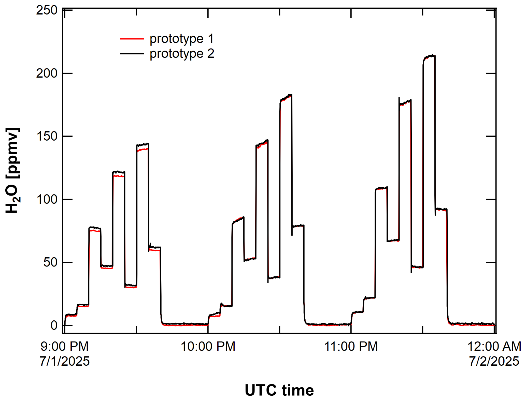
We have performed a direct comparison of our two prototype instruments by operating them in series gas flow during a period of 5 d. During this time, prototype 1 operated continuously, and prototype 2 operated with extended pauses during which other tests and tasks were performed. In total, both instruments operated for 63 h simultaneously. Unfortunately, our DPG became unreliable, and we changed the setup of Fig. 5 such that we added laboratory air with variable humidity to the UZA via a flow controller in the same series of steps. While this setup does not provide a reference humidity, it is well suited to compare the two prototype instruments. A short section of the data taken in this experiment is shown in Fig. 10. As previously we calculated average H₂O values for every step of the dilution ramp, i.e. 9 average values per hour (not shown in Fig. 10).

Figure 10 Section of data of both prototype systems operating in gas-flow series.

In a first step of our analysis, we performed a direct comparison of the average H₂O measurements of the two prototypes as shown in Fig. 11. A linear fit was performed that gave an excellent average agreement between the two sensors of 0.997 ppmv ppmv⁻¹ with a very low zero offset of 0.109 ppmv.

We quantified the agreement between the two sensors further by calculating the point-by-point difference. Figure 12 shows the histogram of this difference for all 568 average data points spanning a H₂O range of 0 to 213 ppmv. The average difference was −0.061 ppmv, and the standard deviation was 1.492 ppmv. The box plot of the difference provides a visual representation of the data distribution, where the box represents the 25 % and 75 % quantiles, and the whisker lines show the standard deviation. The thick vertical line represents the median (−0.023 ppmv) For 50 % of the N=568 averaged data points the two systems agreed to within ±1 ppmv (Q25 to Q75), and for 68 % to within ±1.5 ppmv (±1σ).

We note that neither sensor has been calibrated prior or after the experiments, and both sensors were not temperature controlled in any way and exposed to temperature changes of up to 8 °C d⁻¹. This level of accuracy at low mixing ratios enables reliable determination of RH_i thresholds critical for predicting whether contrails will persist or evaporate.

Figure 11 Direct prototype system intercomparison. The average agreement was 99.7 % with a very low zero offset of 0.109 ppmv.

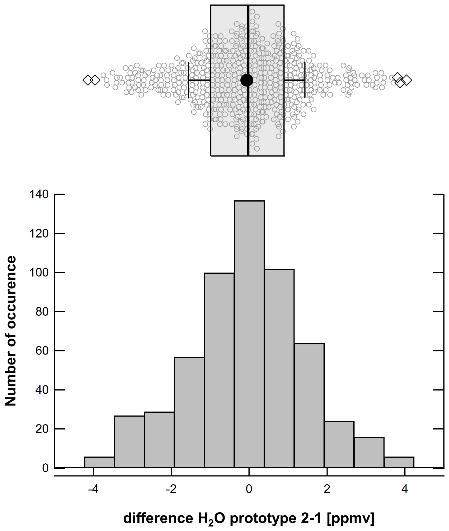
Figure 12 (bottom) Histogram and box plot of the difference (prototype 2 – prototype 1) of averaged H₂O measurements. (top) Box plot of the difference data indicating median (thick vertical line), average (solid marker), 25 % and 75 % quantiles (box), vertical lines (±σ).

3.6 Stability

We have quantified the prototype instrument stability using the data obtained during the 5 d period discussed in the previous section. To do so, we have performed linear fits of the 9 measured H₂O average data of every hour and derived the slope, the offset, and the goodness of the fit (r²). These metrics are shown in Fig. 13. The initial 12 h of the test resulted in an agreement of 0.96 to 0.98. After the initial 12 h we have implemented an improved laser-scan setup to prototype 2, which included repositioning the absorption line and changing the polynomial order of the baseline and it resulted in a slope between the two instruments closer to 1 (top panel of Fig. 13). This type of adjustment is a routine task in the build process of any Aerodyne laser spectrometer. For the remainder of the test the scan setup was not changed, and we achieved an agreement (slope) of 1.004±0.011 ppmv ppmv⁻¹ (avg ± sdev) as indicated by the thick horizontal line and the shaded area between the dashed lines. During the same time the zero offset was $-\mathrm{0.057}\pm \mathrm{1.08}$ ppmv. These results are in excellent agreement with our assessment of the accuracy of our prototype 1 using the DPG absolute humidity scale (Fig. 8), where the slope changed by around 1 % during a 50 h long test. We assume that the instrument drift of both systems has no common-mode term, and thus stability within 2 % between the two independent instruments was expected. The demonstrated stability over multi-day operation without temperature control supports integration into long-duration flight missions and routine operations without onboard recalibration.

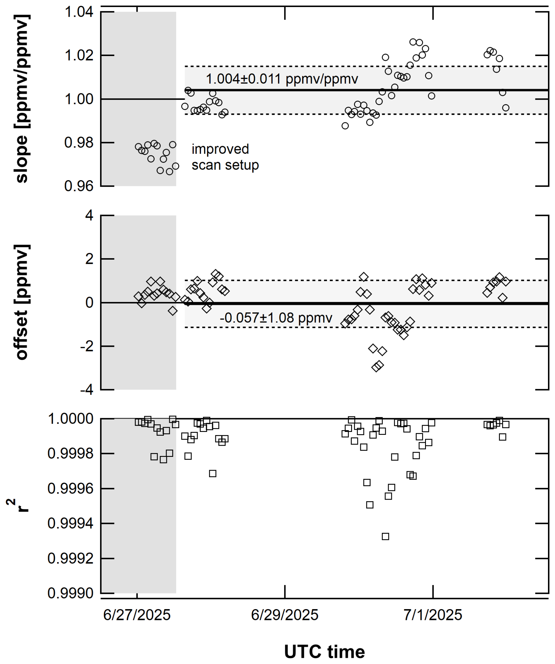
Figure 13 Direct prototype system intercomparison showing hourly (top) slope, (middle) zero offset, and (bottom) goodness of linear fit. Average and standard deviations of slope and offset for the improved laser-scan setup are given in the figure.

3.7 Extended humidity range

We have tested the linearity over a humidity range spanning four orders of magnitude. While the focus for our humidity probe is the humidity relevant for contrail cirrus formation (H₂O <150 ppmv) our sensor also supports much higher humidity measurements. For the high humidity range, we have measured the undiluted output of the DPG. We have changed the temperature setpoint of the DPG between 2 and 20 °C to generate H₂O between around 6900 and 23 000 ppmv. We measured at each DPG temperature for around 5 to 10 min and calculated the average value for each level. The results are shown in Fig. 14 together with H₂O measurements of the low humidity range obtained by diluting the DPG output into UZA. For prototype 1, we found that the measured H₂O showed non-linearity above around 7000 ppmv. We were familiar with such an effect from our commercial mid-IR TILDAS instruments, where optical-power dependent saturation of the detectors causes non-linearity of the retrieved gas concentration. We have thus experimented with attenuating the optical power incident on both the sample and the baseline detectors by adding either a 50/50 or a 25/75 fiber-based y-splitter (YS) upstream of the existing 50/50 y-splitter of our fiber assembly (YS in Fig. 1). Using either the 50 % or the 25 % output port of the additional YS generated a 50 % or 75 % attenuation of the optical power. We have then repeated the undiluted H₂O measurements with prototype 1 and found that the attenuation mitigated the non-linear response of our sensor. With 75 % attenuation we were able to extend the linear range to around 15 000 ppmv. The measurements above 15 000 ppmv showed remaining non-linear response, but this can in principle be included in a calibration. Prototype 2 showed much better linearity as shown by the blue data markers in Fig. 14 (inset). It almost matched the linearity of prototype 1 at 75 % attenuation. The absolute power levels on the detectors of both prototypes were similar, where prototype 2 had around 25 % less optical power on both detectors. This may explain some of the better linearity of prototype 2 but not all in our opinion. Both detector pairs (sample and baseline) of the two prototypes were purchased at different times of the development phase and likely come from different manufacturing batches, which may explain the differences in their response.

We note that the linearization by attenuation increased the noise at contrail-relevant humidity by around 2.5× to 0.25 ppmv at 75 % attenuation. This expected. Indeed, the observed noise increase from around 0.1 to 0.25 ppmv (prototype 1) is only slightly above shot-noise behavior, where the photon noise (standard deviation) scales proportional to the square root of optical power. Here we observe 2.5× higher noise compared to 4× lower optical power. It was shown in Dyroff (2011) that the near-infrared lasers of the type used here can show near-shot-noise limited characteristics. The accuracy of the measurement is not altered by attenuation.

Figure 14 Measured H₂O by prototype 1 (red) and prototype 2 (blue). The optical power on both detectors of prototype 1 was 1: 100 %, 2: 50 %, and 3: 25 %, that of prototype 2 was 100 %. The low humidity data of prototype 1 and prototype 2 were recorded with the DPG set to 15 and 10 °C, respectively. The inset shows the high humidity range between 5000 and 25 000 ppmv with linear axes.

4 Discussion

In this paper we have demonstrated a new humidity probe for the detection of conditions favoring the formation of persistent aviation contrail cirrus clouds. Our probe is explicitly simple in design. Without calibration the two prototypes built and tested showed excellent agreement against a humidity standard of better than 98 % for the relevant H₂O range below 200 ppm. The agreement between both instruments when operated in series measuring the same sample air was 99.7 %. The stability of both instruments was quantified to be ±1 % (1σ) during a 5 d long period where both prototypes operated without any temperature control. Furthermore, we show that our probes can measure H₂O with linear response over 4 orders of magnitude.

Our instrument measures the H₂O mixing ratio (${\left[c\right]}_{{\mathrm{H}}_{\mathrm{2}}\mathrm{O}})$. The formation of contrails is dependent on the relative humidity with respect to ice (${\mathrm{RH}}_i=\frac{p\cdot {\left[c\right]}_{{\mathrm{H}}_{\mathrm{2}}\mathrm{O}}}{p_{{\mathrm{H}}_{\mathrm{2}}\mathrm{O}\mathrm{sat}}\left(T\right)})$ , which in turn depends on the pressure (p) and temperature (T) of the atmosphere via the temperature-dependent H₂O saturation-vapor pressure ($p_{{\mathrm{H}}_{\mathrm{2}}\mathrm{O}\mathrm{sat}}$). The total uncertainty budget thus includes not only the uncertainty of our humidity probe but also on that of the pressure and temperature measurements provided by the aircraft. The RH_i uncertainty scales directly with p and ${\left[c\right]}_{{\mathrm{H}}_{\mathrm{2}}\mathrm{O}}$. At present, the (static) air temperature of the atmosphere may be measured with an uncertainty of ±0.1 K, while a lower uncertainty is desired (Lee et al., 2023). Assuming the standard atmosphere model (ISO 2533:1975) at 12 km altitude (p=193 hPa, T=217 K) we estimate a RH_i uncertainty of around ±1.3 % for a temperature uncertainty of ±0.1 K calculating $p_{{\mathrm{H}}_{\mathrm{2}}\mathrm{O}\mathrm{sat}}$ by the formulation given in Murphy and Koop (2005). Assuming a 0.2 hPa (1 %) uncertainty of the pressure measurement results in a 1 % RH_i uncertainty. In the laboratory we found a 2 % uncertainty in the measured humidity when comparing against our laboratory humidity standard, leading to a 2 % uncertainty in RH_i if all other parameters were measured correctly. Thus, the uncertainty of our humidity probe (2 %) is on par with the expected uncertainty in RH_i due to pressure (1 %) and temperature (1.3 %) measurements.

We have participated with an early version of prototype 1 in the 2023 EcoDemonstrator airborne campaign onboard the NASA DC-8 aircraft. A total of 12 flights were conducted out of Palmdale, CA (USA) and Everett, WA (USA). Our prototype delivered nearly 100 % data coverage. During the campaign, the instrument was not equipped with a baseline detector, and an early version of the sample cell was installed. In flight, the instrument noise was practically the same (∼0.1 ppmv at contrail-relevant humidity) as determined during the laboratory measurements presented here. The accuracy was not as good as shown during the laboratory measurements with an average moist bias of $\sim \mathrm{20}\mathit{\%}\pm \mathrm{10}\mathit{\%}$ against a reference instrument for several reasons: (1) the determination of the baseline proved difficult due to the lack of the baseline detector adding to the retrieved humidity; (2) suspected small leaks at the instrument (later proven contributing to ∼2 ppmv zero offset) and cabin-air leakage through the aircraft door in front of the sample inlet (very difficult to prove). Furthermore, the early version of the sample cell suffered from interference fringes equivalent to around 1 to 2 ppmv. The instrument response time was good despite a 4 m-long inlet tube. The inlet probe, the inlet tube, and the sample cell were heated. For us the campaign was a learning success in that we have been able to integrate modifications to our humidity probe design that include a much-improved sample cell design and the integration of the baseline detector that drastically reduced the uncertainty.

There have been various dedicated intercomparison campaigns in the past that included both research-grade and commercial instruments. During the AquaVIT campaigns at the AIDA cloud chamber, various research-grade instruments compared as good as ±7 % to ±10 % (absolute humidity) to a reference instrument at upper tropospheric conditions (Fahey et al., 2014; Brunamonti et al., 2025). During airborne intercomparison, the WVSS-II compared to within its specified uncertainty of ±50 % at contrail-relevant humidity to an in-flight reference instrument (Vance et al., 2015). Our prototype instrument uncertainty of 2 % (against our lab standard) falls within the range of agreement of some of the research-grade instruments, though we stress out that we still must perform intercomparisons to a reference instrument. This will be part of future work (see Outlook).

Achieving the high level of accuracy of each prototype required careful setup of the spectroscopic fit, including the laser-dependent tuning rate, the baseline characteristics as well as position and width of the fit window, as is done for any Aerodyne laser spectrometer in production. The tuning rate defines the wavenumber scale of the spectrum to be fit. If it is not correct the calculated Voigt profile will not match the measured lineshape profile and hence lead to a humidity bias. The position of the absorption line, the size of the fit window, and the baseline characteristics (polynomial order, here the remainder after normalization with baseline spectrum) are all relevant to minimizing any humidity bias that may arise from erroneously adding or subtracting area under the fit absorption line. It is important to emphasize that the baseline structure under the absorption line is unknown unless one removes the absorption. This is what we do with the baseline detector, yet slight differences between sample and baseline detector require to include a baseline polynomial. This remaining baseline shape is the largest source of absolute uncertainty of our humidity probes.

Our prototypes were operated exclusively at 213 hPa (160 Torr), though the technology is not limited to this pressure. We chose it as it reflects (approximately) the atmospheric pressure at altitudes where aviation contrails are occurring. In an airborne deployment one could (i) control the pressure to a fixed value, or (ii) let the pressure float with the altitude-dependent atmospheric pressure. While the latter approach may be favorable as it would allow to operate the instrument without a vacuum pump, we have not performed the required test matrix to quantify the accuracy in this scenario.

The prototype drift was very low at ±1 % (1σ) during a 5 d long period. We showed that some of the “drift” was indeed due to limitations in our laboratory humidity-generation system. This is a key result and paved the way for the envisaged unattended deployment of our sensors on commercial or research aircraft. The combination of accuracy, stability, and operational simplicity demonstrated here directly supports the development of automated contrail-avoidance decision-support tools. By providing continuous, reliable humidity measurements in the critical low-ppmv range, our probe enables in-flight detection of ice-supersaturated regions, informing real-time flight path adjustments.

In addition to the excellent accuracy at contrail-relevant humidity, our instrument measured humidity spanning 4 orders of magnitude. We identified a non-linear response of our prototype instruments which we attributed to optical-power dependent saturation effects of the detectors. We presented mitigation strategies by (i) lowering the optical power incident on the detectors, and (ii) calibration for linearization at high humidity. Future work will focus on airborne certification, extended flight testing across seasonal and geographic regimes, and integration with meteorological data streams for real-time contrail-avoidance applications.

5 Outlook

We are now entering the pre-production phase of our humidity probe. We will package the instrument into a 19-inch rack-mountable enclosure (405 mm×460 mm, 4U height maximum) which will be separated into electronics and an optics section. The electronics section will be actively ventilated. The optics section will be heated to 40 °C ±0.1 °C to increase the response time of the H₂O measurement compared to room temperature. We estimate the weight of the pre-production instrument to be around 10 kg. The power requirement will be around 50 W in operation, and <100 W during warmup. We will use only the RedWave electronics system from now on, as it provides a compact, low-noise, and low-power system that is ideally suited for the humidity probe. We will finalize the software package for the RedWave electronics system to include real-time spectroscopic fitting and data visualization. We do not plan to integrate a “switch” for linearizing high humidity measurements mid operation by reducing the incident optical power on the sample and baseline detectors. The instrument response at high humidity may be linearized by calibration. We have not explored this option yet but plan to do so in the future.

We have established a collaboration with an industry client to enable long-term intercomparisons of our humidity probe against state-of-the-art humidity sensors in their laboratory and potentially onboard aircraft. We plan to extend the work presented in this paper to include a complete matrix of humidity and sample pressure ranging from ground level to upper troposphere conditions.

When operated onboard aircraft, our humidity probe will be installed in the pressurized cabin. Outside air will be sampled through a dedicated heated inlet system (not part of this design) and guided to the instrument via heated tubing. The instrument is designed to be operated with or without a pump. The sample pressure may either be actively controlled via a pressure controller when using a pump, or it will be uncontrolled and thus a function of flight altitude when using an inlet probe that produces sample flow via a pressure differential. We expect a faster time response than during our laboratory experiments because the instrument will be operated at higher flow rate (to be determined) and at higher temperature (40 °C). The latter will reduce the desorption of H₂O to the cell and tubing walls that determined the secondary time constant of 25 s in our experiments. We plan to operate the instrument simultaneously detecting the sample and baseline spectra, thus achieving 100 % duty cycle. This will provide complete data coverage along the flight path with ≤700 m resolution at 250 m s⁻¹ cruise velocity.

Our humidity measurements will be converted to relative humidity using the temperature and pressure measurements provided by the aircraft system.