Implementation of a multiresolution analysis method to characterize multi-scale wave structures in lidar data

Extracting gravity wave (GW) perturbations from atmospheric observations relies on background removal techniques whose results may differ depending on the observational type and the spectral characteristics of the chosen method. This variability complicates the intercomparison of GW properties across instruments, sites, and studies. Nighttime averaging provides a simple estimate of the background but may smooth out smaller-scale structures. Spectral filtering enables targeted wavelength extraction, though it can be sensitive to noise and edge effects. Sliding polynomial fit offers flexibility but may suppress relevant signals depending on the polynomial degree. To address this issue, we implement and evaluate a processing method based on multiresolution analysis (MRA), designed to better extract and characterize the background and the multi-scale structures of GWs in lidar temperature and wind profiles. The MRA approach is then evaluated in comparison to these techniques and applied to lidar temperature and wind measurements collected on the night of 20 November 2023 at La Réunion. By decomposing the signal into dyadic vertical wavelength bands and an appropriate choice of corresponding details, the MRA can improve the detection of GW-induced perturbations in the spectral range of 0.8 to 12.8 km vertical wavelength by simultaneous background removal and denoising. We use the variance method as a benchmark for determining gravity waves potential energy (GWPE) and ask the question: “How well do the different filtering techniques compare with the variance method?” Given an overall agreement between our developped MRA and the variance method, we conclude that the MRA can also be used to determine reliable gravity wave kinetic energy (GWKE).

Beyond energy estimation, MRA provides a unique capability to compute kinetic and potential energy profiles for tunable vertical wavelength bands, enabling the characterization of vertical and temporal evolution and interactions between different GW scales. These results establish MRA as a robust and complementary tool for improving GW analyses from lidar measurements, with promising applications to long-term climatologies and multi-instrument observational strategies.

1 Introduction

Atmospheric gravity waves (GW) have become a major focus of research in recent years because of their significant effects on atmospheric dynamics and chemistry (Fritts and Alexander, 2003; Medvedev and Yiğit, 2019). As they propagate, GWs strongly influence large-scale atmospheric processes by modulating both horizontal and vertical momentum fluxes. It is commonly assumed that they have a leading-order influence on the mean circulation in the mesosphere and lower thermosphere and that they also impact the tropospheric and stratospheric circulation (Andrews et al., 1987; Holton and Alexander, 2000; Vallis, 2017). Beyond the atmospheric mean circulation, GW impacts also extend to atmospheric variability and predictability from subseasonal to decadal time scales. Hence it is essential that regional and global atmospheric models describe GWs and their effects with reliable accuracy (Achatz et al., 2024). The ongoing improvement of model resolutions leads to an increasing fraction of the GW spectrum that can be simulated explicitly. Yet, even the highest-resolution numerical weather predictions (NWP) still cannot accurately represent the full GW spectrum, so that they will depend on parameterizations for some time to come (Kruse et al., 2022; Polichtchouk et al., 2022).

Over the past four decades, lidars have proven to be invaluable tools for observing and characterizing propagating GWs in the middle atmosphere (Chanin and Hauchecorne, 1981; Gardner et al., 1993; Wilson et al., 1991; Whiteway and Carswell, 1995; Chane-Ming et al., 2000; Duck et al., 2001; Rauthe et al., 2008; Yamashita et al., 2009; Alexander et al., 2011; Kaifler et al., 2015; Strelnikova et al., 2021; Reichert et al., 2021). Lidar observations can be used to infer long-term trends of the middle atmosphere (Li et al., 2011; Kishore et al., 2014; Khaykin et al., 2017). In particular, lidars provide unique, high-resolution measurements of temperature and wind across the middle atmosphere, with temporal and vertical resolution in the order of 1 min and 100 m respectively. Such measurements are widely used to investigate GW propagation, especially in the mesosphere and lower thermosphere (MLT) region (Liu et al., 2009; Placke et al., 2013; Lu et al., 2015; Kaifler et al., 2015; Chen et al., 2016; Lu et al., 2017; Chane Ming et al., 2023; Vadas et al., 2023; Binder and Dörnbrack, 2024). However, lidars typically produce one-dimensional, nighttime vertical profiles, which limits their ability to resolve the horizontal structure and intrinsic properties of atmospheric waves.

Retrieving GW activity from observations requires isolating wave-induced perturbations from the estimated background state. The wave signal itself spans a broad spectral range, including contributions from tides, planetary waves, and GWs. Depending on the observational technique and data processing approach, the fluctuating atmospheric variables – such as temperature and wind – may be attributed primarily to GWs. However, a major challenge lies in effectively distinguishing GWs from larger-scale perturbations as tides or planetary waves. Over the past several decades, various methods have been developed to extract GW perturbations from lidar-derived temperature and wind profiles. A commonly used technique involves subtracting a nighttime average profile, considered representative of the background, from each individual profile (Gardner et al., 1989; Rauthe et al., 2008; Ehard et al., 2014). Another widely applied method fits a polynomial function to the measured profiles to isolate the perturbation field (Whiteway and Carswell, 1995; Duck et al., 2001; Hertzog et al., 2001; Alexander et al., 2011). A further approach to separating GW contributions from large-scale atmospheric motions involves the use of high- or low-pass filters, with the cutoff wavelength determined by the specific characteristics of the filter (Chane-Ming et al., 2000). For GW analysis, high-pass filters are typically applied in the height domain to eliminate tidal or large-scales waves contribution (Hirota, 1984; Hirota and Niki, 1985; Eckermann et al., 1995; Hertzog et al., 2001).

The sensitivity of GW detection methods varies across the wave spectrum and is also strongly influenced by the capabilities of the observing instrument, particularly lidar systems, where performance depends on factors such as laser power and collection area. In the literature, Gravity Waves Potential Energy (GWPE) is commonly estimated over a wide spectral range; however, comparing results across studies remains challenging. This difficulty arises from the inability to clearly distinguish variations caused by differences in methodology from those driven by geophysical variability (Ehard et al., 2015).

Since the 1980s, wavelet theory has found widespread application in signal and image processing. More recently, in combination with neural networks, it has gained increasing relevance in the field of machine learning (Guo et al., 2022). Wavelet analysis is particularly well-suited for examining nonstationary, multiscale, wave-like structures, as it enables the resolution of spectral characteristics in both time and space. As such, it is a powerful tool for capturing the dynamics of GWs whose signatures are embedded in lidar-derived temperature and wind perturbations (Chane Ming et al., 2023; Reichert et al., 2024; Ungermann and Reichert, 2025). Orthogonal discrete wavelets further allow for the continuous tracking of spectral energy evolution with altitude, making use of the principle of energy conservation to assess vertical variations in GW activity. The linear nature of wavelet analysis also makes it well-aligned with the linear theory of GWs, which describes the wave field as a superposition of monochromatic components. Moreover, wavelet-based methods facilitate the investigation of turbulence-related processes, including energy cascades and nonlinear interactions among structures at different scales. These energy densities diagnostics provide complementary insights into different aspects of GW dynamics, with kinetic energy generally being more sensitive to low-frequency waves than potential energy (Geller and Gong, 2010). In this context, the present study introduces a method based on the multiresolution analysis (MRA). MRA, as formalized by Mallat (1989), was developed through the concept of a filter bank with a pyramidal structure, is an efficient algorithm for fast bi-band discrete wavelet decomposition and is a highly versatile tool that offers several key advantages for the analysis of GWs. It enables efficient signal denoising, multi-scale filtering, and accurate signal reconstruction, making it particularly well-suited for studying the complex, multiscale nature of GWs. GW activity in the middle atmosphere is typically quantified by calculating potential and kinetic energy densities from temperature and wind perturbations, respectively (Li et al., 2023; Brhian et al., 2024; Wüst et al., 2025).

Beyond perturbation-based methods, Mzé et al. (2014) proposed an alternative approach for estimating potential energy directly from raw lidar photon count profiles. This method builds on the variance-based technique originally developed by Hauchecorne et al. (1994), allowing GWPE to be inferred without requiring explicit background subtraction.

In this paper, we present a method based on MRA to characterize multi-scale GWs in lidar observations. Specifically, the study aims to compare MRA with commonly used background removal techniques such as nighttime average, sliding polynomial fit and spectral filtering, in order to evaluate their ability to isolate GWs perturbations.This ability is quantified by deriving profiles of GWPE which are compared to GWPE profiles based on the variance method by Mzé et al. (2014). For this analysis, we use lidar temperature measurements from one night in November 2023 at La Réunion. How well does GWPE based on our developped MRA method agree with the established variance method? In a subsequent step, we also compare gravity waves kinetic enery (GWKE) profiles based on co-located lidar wind measurements.

A central motivation for this work is that, while MRA does not necessarily outperform other methods in every aspect, it provides a unique analytical framework that combines multi-scale decomposition with energy conservation, allowing the tracking of spectral energy across different vertical scales. This capability enables the investigation of interactions between wave components of different scales, which is not possible with conventional filtering approaches.

Our work aims to analyze how each filtering technique impacts GW energy profiles and highlights how MRA, energy-conserving framework can complement existing techniques for characterizing atmospheric GWs.

The paper is organized as follows: Sect. 2 describes the lidar datasets and the four filtering approaches, with a focus on the implementation of MRA and a parallel on variance based method. Section 3 presents the results of the systematic comparative analysis for temperature and wind, with a demonstration of MRA's distinctive features using wind data. Section 4 provides conclusions and outlines future applications of the MRA technique.

2 Materials and Methods

2.1 Lidar data

Since 2013, the Rayleigh-Mie-Raman (RMR) lidar and the Rayleigh-Mie-Doppler (RMD) lidar have both been operating at the Maïdo Observatory on La Réunion (21° S, 55° E). The RMR lidar provides vertical profiles of temperature spanning the middle atmosphere, covering altitudes between 30 and 90 km (Baray et al., 2013). Lidar temperature measurements are useful for the study of the middle atmosphere especially for the characterization of multi-scale dynamical processes such as mesospheric inversion layers and GWs (Bègue et al., 2017; Chane Ming et al., 2023). Additionally, horizontal wind velocities are measured by the RMD lidar at heights ranging from 5 to 60 km (Khaykin et al., 2018). Lidar data are primarily used for long-term monitoring of the middle atmosphere and have also supported recent calibration activities, such as those conducted for the European Space Agency's ADM-Aeolus satellite mission dedicated to global wind observations (Ratynski et al., 2023).

Rayleigh lidar operates by measuring atmospheric density, which is directly proportional to molecular Rayleigh scattering, and calculates temperature through the downward integration of the hydrostatic law (Hauchecorne and Chanin, 1980). The light source of this lidar consists of two Quanta Ray Nd:Yag lasers. The final wavelength emitted is 355 nm with a pulse repetition at 30 Hz and each pulse delivers 375 mJ. The backscattered signal is collected by a 1.2 m diameter telescope (Gantois et al., 2024). The temperature profile is initialized at the top using a seed temperature from the NRLMSISE-00 empirical atmospheric model (Picone et al., 2002). Initially, raw Rayleigh-Mie-Raman (RMR) temperature profiles are obtained with a 1 min integration time and a vertical resolution of 150 m. To enhance the signal-to-noise ratio, vertical smoothing and time binning are applied according to the scientific objectives. For example, for nightly mean profiles available on the NDACC database, a 2 km vertical smoothing is applied using a Hanning filter to reduce noise and improve data accuracy.

The horizontal wind components are determined by measuring the Doppler shift between the emitted and backscattered light, induced by the projection of molecular or particle velocities along the laser's line of sight, which is inclined off-zenith. To capture both wind components, the laser beam is alternately directed along the zonal and meridional directions with a 45° elevation. A vertical pointing configuration is also employed to establish the zero Doppler shift reference, based on the assumption that vertical wind velocities are negligible (Chanin et al., 1989; Souprayen et al., 1999). The Doppler lidar uses a Nd:YAG laser operating at 532 nm in monomode. The pulse repetition rate of the laser is 30 Hz with 24 W mean energy. The 0.3 m² telescope of Maido wind lidar is composed of a single rotating mirror, which serves for both the emission and reception. The initial Rayleigh-Mie-Doppler wind profiles are retrieved with a temporal resolution of 5 min and a vertical resolution of 200 m (Khaykin et al., 2016, 2018).

The present study uses individual lidar temperature and wind profiles of 15 min integration time and resampled to a vertical resolution of 100 m to characterize GWs with vertical wavelengths and observed periods > 1 km and 1 h respectively. Lidar measurements are done during the 20 November 2023 night between 15:43 and 20:28 UTC for temperature and between 15:28 and 23:50 UTC for wind (Fig. 1).

Figure 1 Temperature in K (a), zonal wind in m s⁻¹ (b) and meridional wind in m s⁻¹ (c) measurements during the 20 November 2023 night. Waves structures with downward phase progression are visible between 7 and 20 km in Meridional and Zonal wind. This structure is a gravity wave with vertical wavelength of 5 km which we will focus on later.

2.1.1 ERA5 Reanalysis Data

ERA5 (Hersbach et al., 2020) is the fifth generation of atmospheric reanalysis to be produced by the European Center Medium-Range Weather Forecasts (ECMWF). ERA5 dataset is produced using 4D-var data assimilation and model forecasts in Cycle 41R2 of the ECMWF Integrated Forecast System (IFS). The reanalysis provides a large number of parameters, hourly temporal resolution, a horizontal resolution of 0.25° (∼ 31 km), a vertical resolution of 137 levels from ground to 80 km. In order to avoid wave reflections at the model top, two artificial sponge layers are used in IFS: a weak sponge that starts at 10 hPa level, and a stronger sponge that starts at the 1 hPa level. The vertical resolution is ∼ 250 m at heights < 20 km, between 500 and 700 m in the lower stratosphere (24–32 km) and between 1 and 2.5 km at heights of 37–70 km. The model is capable of resolving a broader spectrum of GWs in the troposphere and lower stratosphere with period > 2 h. For the native output grid, the model is capable of resolving GWs with minimum horizontal wavelengths of 60–70 km. However, in order to gain numerical stability, the shortest scales are damped by hyperdiffusion (Preusse et al., 2014; Gupta et al., 2021). At the tropics (equatorward of 20°) GWs with horizontal wavelengths of 300 km are properly resolved by the model (Preusse et al., 2014; Pahlavan et al., 2023).

2.2 Gravity waves analysis techniques

2.2.1 The nighttime average method

The nighttime average background profile is a simple, robust and widely used method for determining background temperature profiles (Gardner et al., 1989; Rauthe et al., 2008; Ehard et al., 2014). This approach assumes that observed periods of GWs are shorter than the measurement period such that phase averaging cancels the GW signal and the nighttime average profile can be assumed to define a thermal background. However, spectral bands of GWs are difficult to define. In our study, the nighttime average background profile is smoothed with a 7.5 km window.

2.2.2 The sliding polynomial fit method

The sliding polynomial fit method consists of performing a local cubic polynomial regression on a sliding window of the vertical profile (Savitzky and Golay, 1964). The polynomial order and the window size are selected according to the vertical resolution of the measurements, making the method equivalent to applying a low-pass finite-impulse-response (FIR) filter with a well-defined frequency (wavelength) response. The height range L of the sliding window and the polynomial order determine the vertical wavelengths that are considered part of the background. Guest et al. (2000) reported that when L is the window size, a 2nd-order polynomial fit may remove perturbations with vertical wavelengths greater than 2L, while a 3rd-order fit may remove those with wavelengths greater than L. Conversely, fits with order higher than 4 may also attenuate inertia–gravity wave signals and should therefore be avoided (Guest et al., 2000).

In our study, we use a window width of 10 km and we fit the subdata to a third order polynomial. Hence, perturbations with vertical wavelengths greater than 10 km are strongly suppressed and associated with the background.

2.2.3 The spectral filtering method

Spectral filtering is another common method to separate GWs from a thermal background by choosing the right cutoff wavelength. Contributions of GWs can be separated from the large scale waves by applying a high/low-pass filter of any cutoff wavelength. Generally, in order to remove low frequency components (or large scale waves) such as tides, high-pass filters are used in the time domain (or height domain) (Hirota, 1984; Hirota and Niki, 1985; Eckermann et al., 1995).

To isolate GW-induced perturbations specifically, the filtering function must be carefully selected to ensure an appropriate spectral response. Chane-Ming et al. (2000) applied a high-pass butterworth filter, with a cutoff of 12 km vertical wavelength, on individual temperature profiles to extract GW perturbations. They, hence, limit the vertical wavelength space to a GW field with vertical wavelengths < 12 km. The Butterworth filter is well adapted for the study of GWs due to its flat frequency response in the passband and is minimizing distortions while effectively isolating the desired wave components.

In this study, we apply a 5th-order Butterworth high-pass filter (Ehard et al., 2015) with a cutoff wavelength of 8 km, allowing us to extract GWs with the observed dominant vertical wavelength of 5 km during the studied night.

2.2.4 The variance method

The variance method, described by Mzé et al. (2014), is a technique used for calculating directly the potential energy of GWs by using raw lidar signal, and is robust against data processing errors (Hauchecorne et al., 1994; Khaykin et al., 2015). The signal originates from an incoherent backscatter lidar operating in photon-counting mode. The raw signal is aggregated over small time and vertical intervals, allowing the vertical profile to be decomposed into a smooth mean profile (background signal) and short-scale perturbations. The relative perturbations, defined as $S^{\prime }(z_i,t_j)=\frac{\mathrm{d}S}{\stackrel{\mathrm{‾}}{S}}$, may arise from either instrumental noise or atmospheric fluctuations (where z_i and t_j are a given altitude and time, respectively). To compute the observed variance and instrumental variance, time-vertical interval (ΔT,ΔZ) are considered by grouping N_t elementary time intervals by N_z elementary altitude intervals as ΔT=ΔtN_t and ΔZ=ΔzN_z. The observed variance, which represents the sum of both instrumental and atmospheric variances, is defined in the time-vertical interval:

$$\begin{array}{}\text{(1)}& V_{\mathrm{obs}}={\displaystyle \frac{\mathrm{1}}{N_t{N}_z}}\sum _{N_z}\sum _{N_t}{S}^{\prime }(z_i,t_j{)}^{\mathrm{2}}\end{array}$$

Since the lidar signal in photon-counting mode follows Poisson's distribution, the instrumental variance can be directly derived from the estimated mean signal S, except in cases of signal saturation due to exceptionally strong returns. The atmospheric variance is then obtained as the difference between the observed and instrumental variances:

$$\begin{array}{}\text{(2)}& V_{\mathrm{atm}}=V_{\mathrm{obs}}-V_{\mathrm{inst}}\end{array}$$

This atmospheric variance serves as an estimator of GW activity in the middle atmosphere and is used in the equation of GWPE (Wilson et al., 1991) as followed:

$$\begin{array}{}\text{(3)}& E_p={\displaystyle \frac{\mathrm{1}}{\mathrm{2}}}{\left({\displaystyle \frac{g}{N}}\right)}^{\mathrm{2}}{V}_{\mathrm{atm}}\end{array}$$

Where V_atm is the equivalent of $({\mathit{\rho }}^{\prime }/{\mathit{\rho }}_{\mathrm{0}}{)}^{\mathrm{2}}$, hence $(T^{\prime }/T_{\mathrm{0}}{)}^{\mathrm{2}}$ in adiabatic and linear conditions; g is earth's gravitational acceleration (m s⁻²); N is the Brunt-Väisälä frequency (s⁻¹).

2.2.5 The multiresolution analysis method

This study focuses on the multiresolution analysis (MRA) based method of which the description of this new method is detailed as opposed to the four previous methods. The MRA framework provides the theoretical foundation for the discrete wavelet transform (DWT), enabling the hierarchical decomposition of a signal into different scales of approximation and detail. It decomposes a signal into orthonormal bases, capturing both coarse approximations and successive details across multiple resolution levels. By adding or removing details, MRA enables a smooth transition between high and low resolutions, with each detail level encoding the differences in information between successive scales. The effectiveness of this approach is further enhanced by its flexibility in constructing orthogonal or biorthogonal bases tailored to the analyzed signal. When combined with efficient algorithms from subband coding theory and filter banks, MRA becomes a robust and adaptive tool for signal analysis (Mallat, 1989; Hubbard, 1998). The original signal is decomposed into successive octave bands (in the dyadic MRA, most widely used), with each level represented by an approximation of order n and discrete details up to that order, forming a pyramid-like wavelet decomposition tree, as described by Mallat's algorithm. Hence, the original signal can be decomposed as followed:

$$\begin{array}{}\text{(4)}& s\left(n\right)=d_{\mathrm{1}}\left(n\right)+d_{\mathrm{2}}\left(n\right)+d_{\mathrm{3}}\left(n\right)+\mathrm{\dots }+d_i\left(n\right)+a_i\left(n\right)\end{array}$$

Where d_i is a detail at the decomposition level i, a_i is the approximation at the decomposition level i and n is the nth element of the data series. The vertical resolution is crucial in this process, as adjusting it modifies the octave band limits, thereby altering the vertical wavelength bands. This adaptability allows for the selective extraction and analysis of GWs at different scales, depending on the chosen vertical resolution. Our method uses the orthogonal Daubechies wavelet which is mostly used in signal reconstruction. This wavelet and its corresponding scaling function of order 8 are sufficiently smooth to provide an optimal balance between computational efficiency and the quality of the decomposed multiscale signals (Chane-Ming et al., 2000; Chane Ming et al., 2023). All lidar profiles are oversampled to a vertical resolution of 100 m, however the study focuses on GWs with vertical wavelengths of 0.8–12.8 km. The 100 m vertical sampling provides different spectral domains corresponding to the wavelength bands: 0.2–0.4, 0.4–0.8, 0.8–1.6, 1.6–3.2, 3.2–6.4, 6.4–12.8 and > 12.8 km.

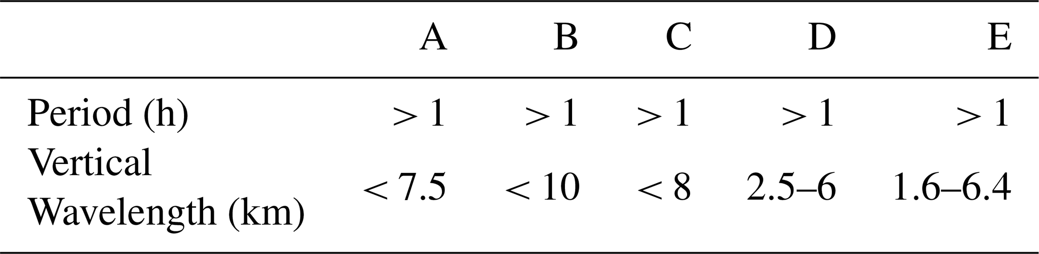
Table 1 summarizes the vertical and temporal passbands associated with the five filtering techniques used in this study. Since the filters are applied only along the vertical dimension of the lidar profiles, no temporal filtering is performed; therefore, wave periods longer than 1 h can be retrieved from the measurements as said in Sect. 2.1. The vertical cutoff wavelengths are selected to be as consistent as possible across methods, allowing for a meaningful comparison of their spectral responses. The different approaches exhibit distinct vertical passbands. The nighttime average (A), sliding polynomial fit (B), and spectral filtering (C) methods remove large-scale variations with cutoff wavelengths between 7.5 and 10 km, effectively isolating shorter vertical wavelengths. The variance-based method (D) targets a narrower band (2.5–6 km), reflecting its inherent design to isolate fluctuations within a defined vertical scale range. In contrast, the MRA (E) selects vertical bands between 1.6 and 6.4 km which corresponds to details d₄ and d₅ of the decomposition. These different passbands are used to derive the GWPE and GWKE of the dominant 5 km wave propagating through the middle atmosphere.

Table 1 Vertical passbands from the different methods presented in this paper: (A) Nighttime average, (B) Sliding polynomial fit, (C) Spectral Filtering, (D) Variance based method and (E) MRA.

GWPE and GWKE (Gravity Wave Kinetic Energy) can be computed from the formulas given in Wilson et al. (1991):

$$\begin{array}{}\text{(5)}& {\displaystyle }{E}_p={\displaystyle \frac{\mathrm{1}}{\mathrm{2}}}{\left({\displaystyle \frac{g}{N}}\right)}^{\mathrm{2}}\stackrel{\mathrm{‾}}{{\left({\displaystyle \frac{T^{\prime }}{T_{\mathrm{0}}}}\right)}^{\mathrm{2}}}\text{(6)}& {\displaystyle }{E}_k={\displaystyle \frac{\mathrm{1}}{\mathrm{2}}}\left(\stackrel{\mathrm{‾}}{{u^{\prime }}^{\mathrm{2}}+{v^{\prime }}^{\mathrm{2}}}\right)\end{array}$$

Where g is the Earth acceleration, N the buoyancy frequency, T₀ the background temperature profile, T^′, u^′ and v^′ are, respectively, temperature, zonal wind, and meridional wind perturbations (the vertical wind is neglected). The overline represents the average over the night of measurements.

The first step for computing GWPE and GWKE is to determine the impact of the Gaussian white noise, present in the temperature and wind profiles, on the MRA decomposition. To do so, we simulate temperature profiles with gaussian white noise 𝒩(0,1) and compute the potential energy of the gaussian white noise. A noise amplitude increasing with the altitude by a factor of $e^{\frac{z}{H}}$, where z is the altitude taken from 20 to 80 km and H is the height scale (8 km), is here considered. Then, the mean energy is calculated on height intervals of 10 km for each detail from the MRA decomposition (level 6) of the 1000 gaussian white noise simulated signals to estimate the impact of the noise on the different spectral bands (Fig. 2).

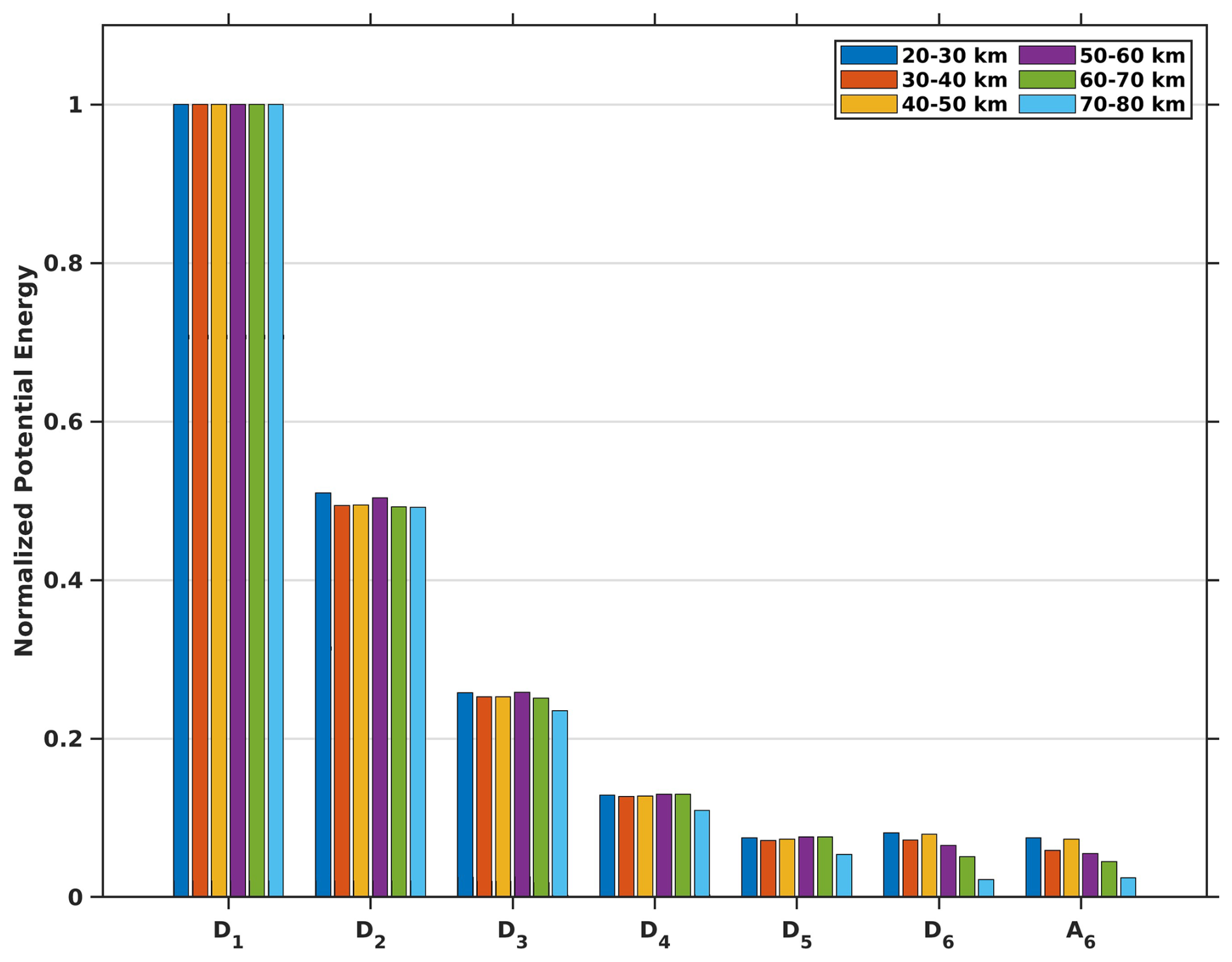
Figure 2 Normalized mean potential energy of 1000 simulated Gaussian white noise signals for each detail level obtained from the MRA decomposition at heights between 20 and 30 km (blue), 30 and 40 km (orange), 40 and 50 km (yellow), 50 and 60 km (purple), 60 and 70 km (green), 70 and 80 km (cyan).

Before analyzing the noise contribution across the MRA levels, the data were oversampled to a 100 m vertical resolution. The original temperature profiles from lidar measurements have a vertical resolution of 150 m, which allows the detection of GWs with minimum vertical wavelengths of approximately 300 m. After oversampling, the first detail level of the MRA corresponds to vertical wavelengths between roughly 200 and 400 m. This interval contains only white noise, as GWs with vertical wavelengths shorter than 300 m cannot be resolved by the instrument.

Although white noise is present at all scales, the dyadic nature of the MRA leads to a progressive reduction of noise energy by a factor of 2ⁿ⁻¹ at the nth decomposition level. This behavior is illustrated in Fig. 2, where the normalized noise energy decreases by a factor of two at each step of the decomposition, under the assumption that the first detail level d₁ contains only noise and it is direct consequence of the pyramidal decomposition of the MRA. We observe that a₆ and d₆ exhibit noise of similar amplitude, as both belong to the same level of dyadic decomposition. This highlights that in multiresolution analysis, noise is distributed equally between the detail and approximation components at a given decomposition level. Consequently, the noise-induced potential energy calculated from d_n, $E_{p_n}$, can be estimated using an empirical formula, assuming that the first detail level of the MRA decomposition ($E_{p_{\mathrm{1}}}$) consists solely of noise: $E_{p_n}=\frac{E_{p_{\mathrm{noise}}}}{{\mathrm{2}}^{n-\mathrm{1}}}$, with n varies from 2 to 6 for a decomposition at order 6, and $E_{p_{\mathrm{noise}}}$ is the equivalent of computing $E_{p_{\mathrm{1}}}$.

The GW energy (potential or kinetic) is computed for each perturbation (temperature or wind) profile of the considered night of measurements. In order to subtract noise, we remove noise energy corresponding to the nth detail treated by applying the empirical formula. Then, the nighttime average profile of the GW energy is determined, and the mean profile is smoothed using a 7.5 km Hanning window. This process enables the estimation of the average propagation of GWs during the night. With the MRA decomposition, it is possible to derive an energy profile that focuses on a dominant or quasi-monochromatic mode of GWs. It enables to highlight the evolution of GW modes and the interaction between them. Due to potential edge effects, the MRA method may bias GW energy as it approaches the upper or lower limits of vertical profiles, depending on the order of the detail and the amplitudes of the signal. To mitigate edge effects, it is recommended to either reduce the vertical range of the decomposed signal for further analysis.

3 Comparison of the different methods

In the following section, we demonstrate the capability of the MRA method to estimate both background and perturbation profiles by comparing its results with those obtained from conventional approaches, including nighttime average, sliding polynomial fit, and spectral filtering. First, the four methods are applied to the temperature profiles to extract background fields and wave-induced perturbations. The resulting GWPE estimates are then compared with those derived using the variance method of Mzé et al. (2014) to assess their relative performance. The same analysis is subsequently carried out using wind profiles, allowing for a direct comparison of the methods across both datasets. Finally, the ratio between GWKE and GWPE is calculated to provide additional insight into GW characteristics during the night. An illustrative case study is presented below.

3.1 Case study: 20 November 2023

The GWPE and GWKE derived from the MRA and conventional methods are illustrated using lidar profiles from the night of 20 November 2023. ERA5 reanalysis data reveal a strong GWs activity clearly visible in zonal wind, meridional wind and stratospheric temperature perturbations over La Réunion (Fig. 3).

Figure 3 Height-time representation of (a) zonal wind (m s⁻¹), (b) meridional wind (m s⁻¹) and (c) temperature (K) perturbations above La Réunion (21.0° S, 55.5° E) derived from ERA 5 reanalysis (Hersbach et al., 2020) from 20 to 25 November 2023. These perturbations are derived from the d₅ detail component of the MRA applied to wind and temperature data. The enhancement of perturbations, especially in the lower stratosphere, might be attributed to the presence of the subtropical jet above La Réunion (21.0° S, 55.5° E). ERA 5 confirms the presence of GW structures which can be seen in all perturbations plots (black boxes).

Vertical profiles of horizontal wind from ERA5 reanalysis (Hersbach et al., 2020) and radiosonde measurements on 20 November 2023 at 12:00 UTC show good agreement and reveal the presence of short-scale GW structures (Fig. B1 in Appendix B). In particular, ERA5 wind profiles display clear stratospheric GW perturbations (boxes on Fig. 3a and b) with an estimated vertical wavelength of approximately 5 km during the night of 20 November 2023 (Fig. 3). To further characterize these features, a hodograph analysis was performed by examining the altitude-dependent evolution of the horizontal wind components. It reveals a GW elliptical structure at heights of 30–35 km with a vertical wavelength of 5 km. The counter-clockwise rotation of the ellipse with height indicates upward energy propagation into the middle stratosphere. The axis ratio of the ellipse provides an intrinsic wave period of about 23 h. Assuming that the dominant GWs propagate primarily in the vertical direction and are detectable at higher altitudes in the lidar profiles, the following sections focus on a detailed characterization of these wave structures.

3.2 Application to lidar temperature profiles

First, the MRA method is evaluated against conventional approaches by comparing the estimation of background temperature, temperature perturbations, and GWPE, using lidar temperature measurements acquired on 20 November 2023 between 15:43 and 20:28 UTC, during an approximately 5 h observation period. Background temperature profiles were derived using spectral filtering with cutoff wavelength at 8 km, sliding polynomial fit with 3rd order polynomial function, nighttime averaging over the 5 h of measurement, and the MRA method (Fig. 4a). In order to isolate GWs with dominant vertical wavelengths around 5 km within the MRA framework, we use the details d₄ (1.6–3.2 km) and d₅ (3.2–6.4 km), of which the sum effectively captures the wave structure. Between 30 and 45 km altitude, the background fields are consistent with each other, except for the ERA 5 temperature profile, which shows a warm bias of about 10 K near 30 km, decreasing progressively with altitude up to 45 km. Near the stratopause, the background obtained using nighttime averaging is approximately 10 K lower than those produced by MRA, spectral filtering and sliding polynomial fit. In contrast, MRA, spectral filtering and sliding polynomial fit methods display consistent and smoother behavior, yielding a more realistic background structure at the stratopause level. The ERA5 temperature profile exhibits a stratopause altitude slightly lower than that observed in the raw lidar measurements. By examining the temperature perturbations (Fig. 4b) obtained by subtracting the background from the original temperature profiles, it is evident that the perturbations derived using the MRA are smoother than those obtained from the conventional methods. Below the stratopause, the perturbation amplitudes are of the same order of magnitude across all methods. However, at the stratopause level, the perturbations obtained using the nighttime average method are almost twice as large as those from the other three methods. The MRA-derived perturbations are less noisy, particularly above 50 km, where GW amplitudes retrieved with conventional techniques can be up to twice as large as those derived with the MRA.

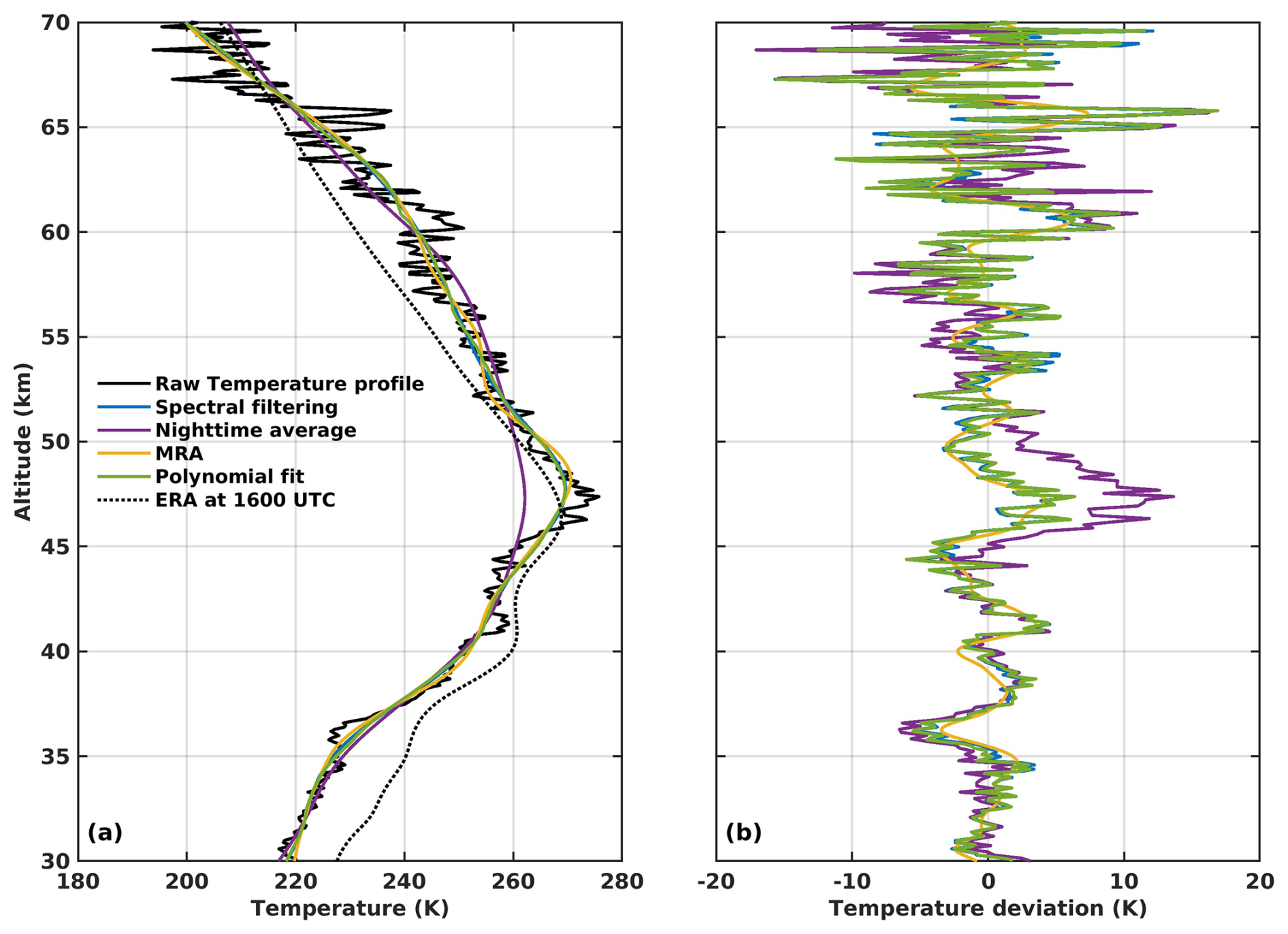
Figure 4 Original temperature profile at 15:43 UTC (black), background temperature retrieved by different methods (a): Spectral filtering (blue), Nighttime average (purple), trend (d₆+a₆) obtained from the MRA (yellow) and 3rd order sliding polynomial (green). The MRA trend corresponds to vertical wavelengths > 6.4 km.

Figure 5 represents the temperature perturbations obtained from all the methods with respect to time and altitude. Across all methods, a distinct wave structure is visible at altitudes between 35 and 45 km. This structure with a downward phase progression (upward energy propagation) is a typical GWs structure and has a vertical wavelength of approximately 5 km (Fig. 5). This feature appears more pronounced in the spectral filtering, the MRA and sliding polynomial derived signals, highlighting the consistency of the MRA approach with conventional techniques. Above the stratopause (47.5 km), waves structures are less visible in height time representation for nighttime average, spectral filtering and sliding polynomial fit methods mainly due to a decrease in signal to noise ratio. Moreover, the nighttime average method produces structures that are inconsistent with GW at these heights. The MRA effectively reveals the 5 km vertical wavelength structure, which is clearly visible in the extracted perturbations. The results closely match those obtained using other background removal methods, particularly the spectral filtering and sliding polynomial fit, which also highlight this wave component. However, the MRA is less sensitive to noise, resulting in improved signal clarity and a higher signal-to-noise ratio. These advantages underscore the effectiveness of the MRA in detecting GWs at this scale, making it a robust and reliable alternative to conventional filtering techniques.

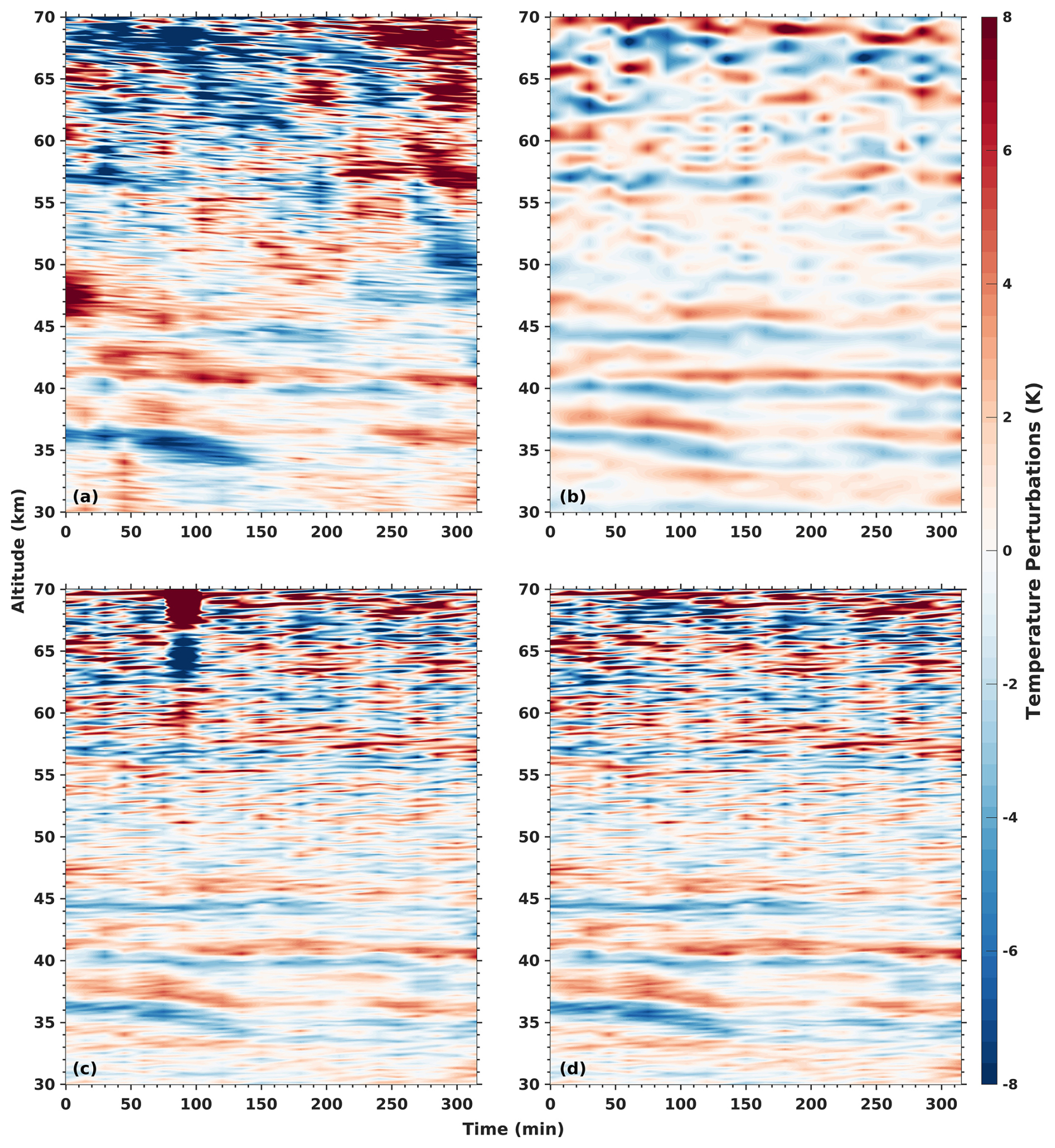
Figure 5 Height-time distribution of the temperature perturbations for 20 November 2023 night obtained from the four methods: nighttime average (a), MRA focused on d₄ (1.6–3.2 km) and d₅ (3.2–6.4 km) (b), spectral filter with a cutoff wavelength of 8 km (c), sliding polynomial fit with 3rd order polynomial (d). Time 0 min corresponds to the beginning of the measurements at 15:243 UTC.

The main focus of the study is the computation of GWPE, using the variance method (Mzé et al., 2014) as a reference in terms of both vertical trends and values. To assess the effectiveness of the MRA approach, we compute the relative errors in GWPE between the variance based method and the other methods (Table 2). In this part of the analysis, the GWPE is evaluated for GWs with a vertical wavelength of 5 km across all methods. Vertical profiles of GWPE derived from the MRA (focusing on details d₄ and d₅), spectral filtering, nighttime averaging, and sliding polynomial fit exhibit similar vertical behaviors to those obtained with the variance method up to approximately 45 km altitude (Fig. 6).

Table 2 Relative error (in %) of GWPE for the different methods, with the variance derived values taken as the reference. Deviations are computed over different altitude ranges from 30 to 70 km.

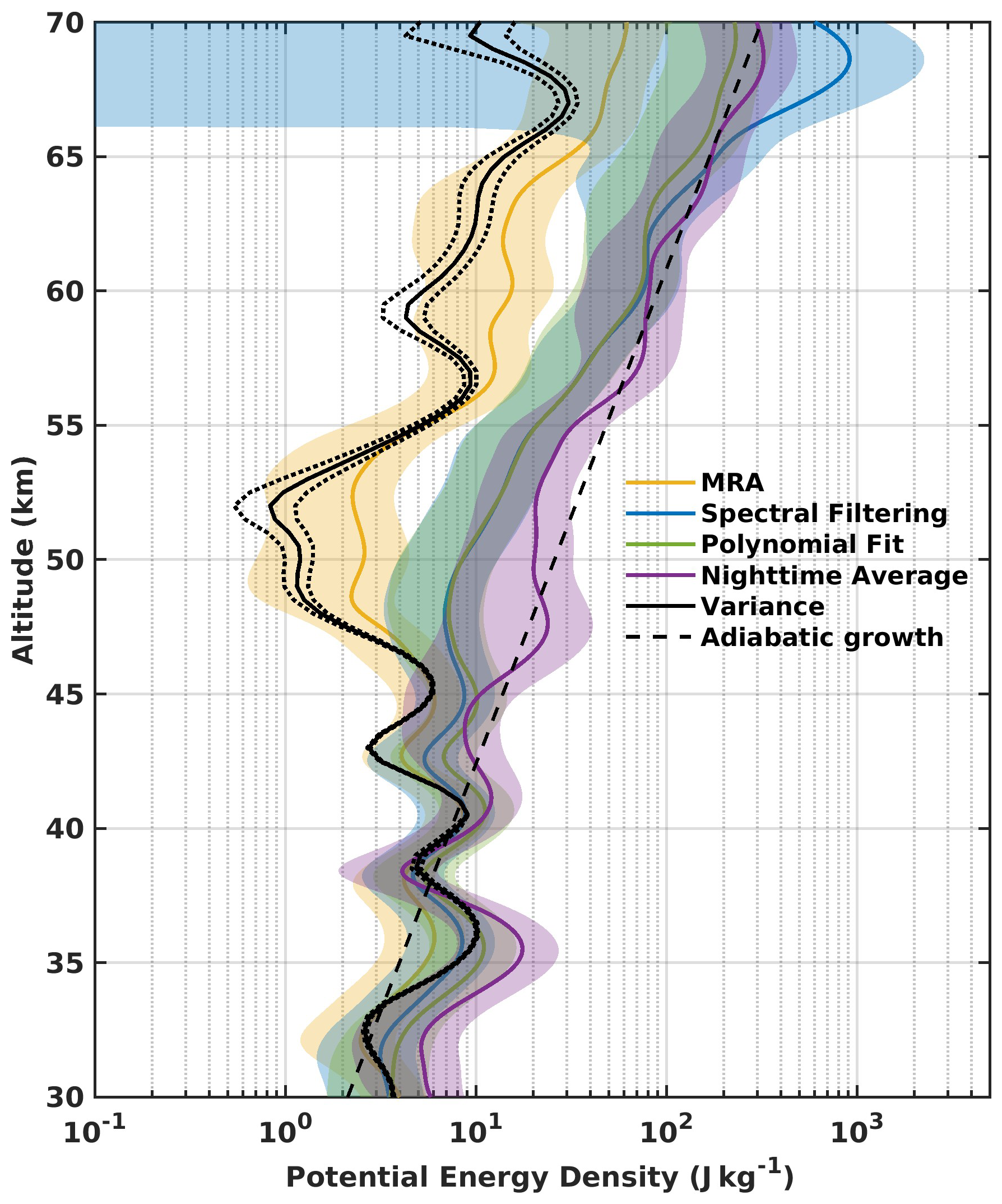
Figure 6 Mean GWPE on the night of 20 November 2023, derived using different methods: variance method (black), MRA (yellow), spectral filter with an 8 km cutoff (blue), night-mean subtraction (purple), and polynomial fit (green). Dotted black lines represent the variance method error, dashed line represent the adiabatic growth, and shaded areas indicate the 95 % confidence intervals.

In addition, the nighttime average profile yields, on average, GWPE values roughly twice as large as those derived from the MRA below the height of 45 km. Above the 45 km altitude, the potential energy profiles begin to diverge: whereas the MRA and spectral filtering methods show a decrease in GWPE, the night-mean and polynomial fit methods instead exhibit an increase. Throughout the altitude range, the GWPE profile deviates significantly from the theoretical adiabatic growth rate (dashed line), indicating continuous energy dissipation or saturation. This strong attenuation leads to a local energy minimum observed at 55 km altitude. The spectral filtering method also detects this minimum, but at slightly lower heights and with GWPE values three to four times higher. In contrast, the night-mean and sliding polynomial fit methods do not capture the minimum and instead yield GWPE values ten times higher than those from MRA. Above 60 km height, the three conventional methods exhibit similar trends, with energy values exceeding the expected density decrease, highlighting the impact of noise on the energy profiles. Meanwhile, the MRA-derived GWPE profile closely follows the decreasing density curve.

At heights between 30 and 50 km altitude, GWPE values from the MRA method agree with the variance method to a relative error less than 20 % in average.

The GWPE profile derived from the MRA also mirrors the overall trends observed with the variance method: an increase between 30 and 40 km, followed by a decrease to a minimum around 50 km, and then a rise above 52.5 km, consistent with the expected exponential growth linked to the decrease in atmospheric density. Notably, near 50 km altitude, the MRA energy profile shows values approximately 60 % higher than those of the variance method (Table 1); however, the variance method's estimates remain within the MRA's 95 % confidence interval. Between 30 and 40 km, spectral filtering, sliding polynomial fit and nighttime average methods have values 13 %, 24 % and 67.5 % higher respectively to those derived from the variance. This relative error is increasing with respect to altitude, corresponding to the decrease of the signal to noise ratio mentionned previously. Hence, the noise has a strong impact on GWPE derived from conventional methods. Overall, the MRA demonstrates strong agreement with the variance method, highlighting its reliability in estimating GWPE. The noise handling in the MRA method allows for a more accurate estimation of GWPE, particularly in the mesosphere.

3.3 Application to lidar wind profiles

Wind measurements obtained from lidar rely on determining the phase shift of the Doppler signal. As a result, it is not possible to apply a variance-based method to directly estimate kinetic energy from wind lidar data. The results presented in the previous section demonstrated the effectiveness of the MRA approach for analyzing GWs in temperature profiles, showing better agreement with the variance method than conventional techniques. Applying the MRA to wind lidar profiles successfully isolates perturbations with a vertical wavelength of around 5 km from detail coefficients d₄ and d₅.

At heights between 7 to 30 km, the GW pattern is clearly visible across all zonal wind perturbations, regardless of the method used (Fig. 7). Between 7 and 15 km, gravity wave structures are visible in all perturbation fields derived from the different methods. However, amplitude enhancements in this altitude range are more pronounced for the spectral filtering and sliding polynomial fit methods (Fig. 7c, d), whereas the MRA and nighttime averaging methods (Fig. 7a, b) exhibit less amplification. Above 30 km, small-scale perturbations not related to GW appear in the results from the spectral filtering and sliding polynomial fit methods (Fig. 7c, d). In contrast, the MRA-derived perturbations still exhibit coherent GW signatures in this altitude range. The nighttime averaging method (Fig. 7a) shows limitations above 30 km height, where it struggles to properly estimate GW perturbations and background winds in the upper stratosphere–lower mesosphere (30–60 km) region.

Figure 7 Height-time distribution of the zonal wind perturbations for 20 November 2023 night obtained from the four methods: nighttime average (a), MRA focused on d₄ (1.6–3.2 km) and d₅ (3.2–6.4 km) (b), spectral filter with a cutoff wavelength of 8 km (c), sliding polynomial fit with 3rd order polynomial (d). Time 0 min corresponds to the beginning of the measurements at 15:28 UTC.

In the following results, we compare GWKE derived from the different methods. Nevertheless, we compute GWKE for the different details of MRA, corresponding to specific vertical wavelengths bands. Figure 8 represents the mean GWKE over the night of measurement for MRA d₂ to d₅ (d₆+a₆ is considered as background), spectral filtering, nighttime average and sliding polynomial methods.

Figure 8 Mean GWKE on the night of 20 November 2023, derived using the different methods: nighttime average method (purple), spectral filtering (blue), sliding polynomial fit (green), d₂ (0.4-0.8 km, brown), d₃ (0.8–1.6 km, red), d₄ (1.6–3.2 km, light blue), d₅ (3.2–6.4 km, yellow). Shaded areas indicate the 95 % confidence intervals.

At altitudes between 10 and 15 km, an enhancement of GWKE is observed across all methods. This increase is most pronounced for the smaller-scale GWs (details d₂, d₃, and d₄). Such an enhancement may be associated with the subtropical jet, which is known to generate small-scale GW (Plougonven and Zhang, 2014). Conventional approaches do not explicitly separate contributions from different vertical wavelengths, so while the enhancement is still visible, it appears less amplified than in the MRA results. Above 15 km, the GWKE associated with details d₂, d₃, and d₄ increases steadily up to 30–35 km. A similar increase is observed for the conventional methods, showing a coherent growth up to around 30 km, after which their GWKE profiles begin to diverge. The GWKE derived from the nighttime average method continues to increase, whereas the spectral filtering and sliding polynomial fit methods show a slight decrease up to approximately 40 km. In contrast, the GWKE associated with detail d₅ decreases within this altitude range. Above 45 km, the GWKE for d₄, d₅, spectral filtering, and sliding polynomial fit starts to increase again, while the kinetic energy for d₂ and d₃ continues to decrease. The MRA results also highlight a connection between GW with vertical wavelengths of 0.4–1.6 and 3.2–6.4 km, suggesting possible interactions between smaller- and larger-scale waves. Such interactions cannot be inferred from the conventional approaches, where the GWKE associated with smaller-scale GW is mixed with that of the dominant 5 km waves, preventing their separation. In terms of GWKE values, clear differences between the methods are observed depending on altitude (Table 3). In the 10–20 km height range, GWKE obtained from spectral filtering, sliding polynomial fit, and nighttime averaging methods are approximately 76 %, 130 %, and 12 % higher, respectively, than the GWKE derived from MRA details d₄ and d₅. Between 20 and 30 km, GWKE from spectral filtering and sliding polynomial fit shows better agreement with MRA, with values about 70 % and 81 % higher, respectively. In contrast, GWKE derived from the nighttime averaging method is almost 150 % than GWKE derived from MRA. Above 30 km, the GWKE from the nighttime averaging method starts to diverge strongly, exceeding MRA-derived values by more than 600 %, with the overestimation continuing to grow into the lower mesosphere. In the same altitude range (30–40 km), spectral filtering and sliding polynomial fit methods overestimate GWKE by more 200 %. Beyond this layer, the relative differences decrease to approximately 70 % for spectral filtering and 100 % for the sliding polynomial fit method.

Table 3 Relative error (in %) of GWKE for the different methods, with MRA-derived values (from d₄ and d₅) taken as the reference. Deviations are computed over different altitude ranges from 10 to 60 km.

The ratio of kinetic to potential energy (hereafter ER) was computed for three altitude intervals: 30–40, 40–50, and 50–60 km, using the different methods and the MRA detail coefficients d₂, d₃, d₄, and d₅ (Fig. 9).

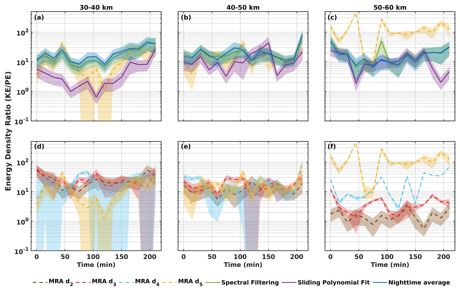
Figure 9 Energy ratio (GWKE $/$ GWPE) computed for nighttime average method (purple), spectral filtering (blue), sliding polynomial fit (green), MRA details d₂ (brown), d₃ (red), d₄ (light blue), d₅ (yellow) during the 20 November 2023 night between 30–40 km (a, d); 40–50 km (b, e) and 50–60 km (c, f). Shades represent the uncertainty error.

Between 30 and 40 km, the ER exhibits similar values and temporal behavior for the spectral filtering, sliding polynomial fit, and MRA methods. A pronounced minimum (ER ∼ 1) is observed for MRA detail d₅. In contrast, the ER derived from the nighttime average method shows incoherent values compared to the other approaches, but gradually increases from about 100 min after the start of the measurements (15:43 UTC) until the end of the night. Between 40 and 50 km, the ER derived from all methods shows comparable values (around 15–20) and similar temporal trends, except for the nighttime average method, which exhibits larger variability. Oscillations are observed in the ER for all methods. These oscillations may reflect the modulation of gravity wave activity by GWs with short periods (∼ 1 h). Between 50 and 60 km, the ER values obtained from spectral filtering, sliding polynomial fit, and nighttime averaging remain broadly similar, but are lower than those found in the stratopause region. In this lower mesosphere layer, the conventional approaches yield ER values close to 10. In contrast, the ER from MRA reaches values of around 100, indicating a predominance of kinetic over potential energy and revealing a different behavior for the dominant 5 km vertical wavelength GWs. The MRA results thus highlight a change in wave frequency as they propagate through the middle atmosphere.

For the MRA details d₂, d₃, and d₄, the ER slightly decreases from 30–40 to 40–50 km, whereas it increases for detail d₅ over the same altitude range. From 40–50 to 50–60 km, the ER decreases for the smaller vertical wavelengths (d₂, d₃), but increases for the larger vertical wavelengths (d₅, d₄). This evolution reflects the modification of the GW frequency distribution with altitude (Wilson et al., 1990). The increase in ER observed for detail d₅ suggests a transition toward lower-frequency GW, where the kinetic energy component tends to dominate over the potential energy (Geller and Gong, 2010).

Overall, the MRA highlights features of GW propagation through the middle atmosphere that remain hidden when using conventional approaches. In particular, MRA brings to light interactions between different wave scales during propagation. A transfer of momentum from smaller- to larger-scale GWs may occur, potentially indicating the presence of secondary wave sources in the middle atmosphere.

4 Summary, conclusions and perspectives

This study implemented a multiresolution analysis (MRA) with the 8th order Daubechies wavelet to investigate GWs from lidar observations at La Réunion. We compared MRA with three conventional background removal techniques, nighttime average subtraction, sliding polynomial fit, and spectral filtering, and used the variance method (Mzé et al., 2014) as a reference for GWPE. A case study on 20 November 2023, exhibited pronounced GW activity. ERA 5 reanalysis also shows coherent wind and temperature perturbations over La Réunion from 20 to 25 November, providing independent support for the observed wave signatures.

The primary differences between the approaches arise from their distinct vertical spectral passbands. The nighttime average method, widely used to estimate background temperature or wind by time averaging over the measurement period, is sensitive to all variability occurring on the timescale of the observations, including contributions from planetary waves and tides. Because the duration of nighttime measurements can vary substantially from one night to another, the portion of the GW spectrum retained after background subtraction may likewise vary between nights. In our implementation, applying a 7.5 km Hanning window provides a consistent vertical cutoff, systematically filtering perturbations with vertical wavelengths > 7.5 km.

The sliding polynomial fit method involves performing a local cubic polynomial regression on a sliding vertical window. The polynomial order and window size must be carefully selected according to the vertical resolution of the measurements, as these parameters determine the effective spectral response of the filter. Consequently, the method requires tuning whenever the vertical resolution of the data changes.

As an alternative, spectral filtering using a Butterworth filter offers a more straightforward and flexible approach. This technique is not dependent on the vertical resolution of the profile and allows easy adjustment to any desired cutoff wavelength, while remaining simple to implement.

Conceptually, MRA is equivalent to applying a bank of band-pass filters, but it offers several distinctive advantages. The choice of wavelet and vertical sampling determines the position and width of the dyadic bands, thereby controlling the amplitude response of each scale. Changing the wavelet affects the spectral response and can modify the retrieved GW amplitudes. For lidar applications, previous studies have shown that the Daubechies wavelet at order 8 is well adapted for the analysis of GW perturbation in the middle atmosphere (Chane-Ming et al., 2000), which motivated its use in this study.

Beyond this filtering analogy, a key strength of MRA lies in its orthonormal decomposition, which ensures that the total signal energy is exactly partitioned across the different scales. This property enables energy-conserving reconstruction of GW perturbations, providing a physically consistent way to examine wave energetics across scales – something that sliding polynomial fit and standard spectral filters do not guarantee. Furthermore, MRA provides simultaneous spatial and spectral localization, allowing the tracking of GW structures and their energy distribution as they evolve with altitude. This makes it particularly well suited for studying multi-scale interactions, such as energy transfer between wave components, which are difficult to isolate with conventional filtering techniques.

All approaches were applied to temperature and wind lidar data with close vertical cutoff in order to identify the dominant GW structure with ∼ 5 km vertical wavelength. In our study, the different approaches consistently identify this dominant GW structure; however, their behavior diverges with increasing altitude and decreasing signal-to-noise ratio. Conventional methods are simple and effective in the lower stratosphere, but they are more susceptible to noise above ∼ 50 km, and mix contributions from different vertical wavelengths, which can bias energy estimates. In contrast, MRA yields smoother perturbations at high altitudes, provides sharper vertical time localization, and produces multi-scale diagnostics within a single, coherent framework. GWPE from MRA agrees well with the variance method up to ∼ 45–50 km and follows the expected density scaling at higher levels, where conventional methods increasingly overestimate energy due to noise.

To deepen the understanding of GW propagation from their generation in the lower atmosphere to their dissipation and breaking in the middle atmosphere, MRA provides a unique framework to calculate scale-resolved energy profiles. Both kinetic and potential energy densities can be estimated for each detail, corresponding to tunable vertical wavelength bands defined by the dyadic wavelet decomposition. This approach yields a consistent and energy-conserving quantification of how GW energy is distributed across scales.

In addition, computing the kinetic-to-potential energy ratio within specific altitude ranges allows the characterization of the vertical evolution of wave frequency distribution and intrinsic properties. Such diagnostics provide insight into processes such as filtering, dissipation, and scale-dependent changes in wave energetics.

A further strength of the MRA is its ability to reveal interactions between wave components of different scales, which remain largely hidden with conventional filtering techniques. This highlights its potential to capture momentum transfers and secondary wave generation processes, offering new perspectives on how GW shape the dynamics of the middle atmosphere.

Extending the study to include the troposphere, through the integration of radiosonde data or reanalysis outputs, could help identify GW properties linked to their specific sources such as tropical cyclones during austral summer. Since GW characteristics depend on their generation mechanisms and the way they interact as they propagate, this multi-scale perspective is especially valuable. Future observational strategies should aim to combine lidar measurements with complementary instruments such as radiosondes, satellite sounders, or GNSS radio occultation profiles. Such multi-instrument synergy could provide a more complete and nuanced view of GW propagation and vertical energy transfer in the atmosphere.

Appendix A: Sensitivity study

A1 Vertical Resolution and Associated Vertical Wavelength Bands

As mentioned in the main text, vertical wavelength bandwidths used in MRA can be adjusted by resampling our data with a new vertical resolution. Table A1 summarizes the vertical-wavelength bandwidths associated with each decomposition level for different vertical resolutions. The choice of vertical resolution directly controls the range of GW vertical wavelengths that can be detected, with the smallest detectable wavelengths scaling with the sampling interval. In every cases, the smallest detectable wavelength is at least 2×d_z where d_z is the vertical resolution. As the vertical resolution increases from 0.1 to 0.25 km, all vertical wavelength bands are progressively shifted toward the details of higher order, leading to a loss of sensitivity to small-scale structures (small-scale structures corresponds to the d₁ and d₂, hence structures with vertical wavelengths < 1 km). Consequently, the physical interpretation of the decomposition levels depends on the selected vertical resolution. In addition, the approximation component (a₆) encompasses increasingly larger wavelengths for coarser resolutions. In this case, larger scale phenomena may not be filter out from our signal (tides or planetary waves for instance).

Table A1 Vertical wavelengths bandwidths (in km) associated with the decomposition level for different vertical resolution dz.

Figure A1 GWPE profiles for details d₄ and d₅ derived from the MRA using Daubechies wavelet at order 4 (blue), 8 (purple), 12 (green) and 20 (orange). The GWPE variance profile is also plotted to have a reference.

A2 Wavelet Order and Effects on GWPE and GWKE

The choice of the wavelet order (i.e., Daubechies wavelet) has a significant impact on the resulting gravity wave potential energy (GWPE) profiles. Figure A1 shows GWPE estimates derived from the d₄ and d₅ detail components (corresponding to vertical wavelengths between 1.6 and 6.4 km for dz=100 m), obtained using Daubechies wavelets of order 4, 8, 12, and 20. The variance profile is included as a reference. Below 50 km altitude, GWPE obtained from the MRA are comparable for all tested wavelet orders. Above this altitude, significant discrepancies emerge. In particular, GWPE derived using the db20 wavelet is strongly overestimated above 50 km and does not provide a realistic representation of GW energy. A similar behavior is observed for the db12-derived GWPE around 60 km. In contrast, GWPE profiles obtained using db4 and db8 remain in good overall agreement throughout the altitude range considered. To further quantify these differences, the relative error of the GWPE estimates obtained with each wavelet order was evaluated. Below 50 km, db20 yields the smallest relative error, with a 15 % overestimation, compared to 16 %, 17 %, and 26 % for db8, db12, and db4, respectively. Above 50 km, db20 exhibits the largest relative error, exceeding 5000 %, whereas relative errors of approximately 85 %, 91 %, and 879 % are obtained for db4, db8, and db12, respectively. Based on this analysis, the db8 wavelet provides the most robust compromise for applying MRA to characterize GWPE and GWKE over the full altitude range.

GWKE estimates derived from the MRA exhibit broadly similar vertical structures for all tested wavelet orders (Fig. A2). However, noticeable discrepancies are observed, particularly between 15 and 20 km altitude, where GWKE derived using the db20 wavelet is markedly overestimated, while GWKE obtained with the db4 wavelet is underestimated. In addition, the altitude at which dissipation becomes apparent differs among the wavelet orders. Dissipation onset is identified at approximately 45 km for db20, at 50 km for db4 and db12, and at 55 km for db8. These results demonstrate that the choice of wavelet order can significantly influence the inferred vertical distribution of GWKE and, consequently, the resulting geophysical interpretation.

Figure A2 GWKE profiles for details d₄ and d₅ derived from the MRA using Daubechies wavelet at order 4 (blue), 8 (purple), 12 (green) and 20 (orange).

Appendix B: ERA 5 and Radiosonde Wind Profiles

Figure B1 presents the zonal and meridional wind profiles over La Réunion from 20 to 23 November 2023 at 00:00 UTC. A good agreement between ERA5 reanalysis and radiosonde observations is observed from the surface up to approximately 35 km altitude. However, small-scale perturbations with vertical wavelengths shorter than 1 km are not captured in the ERA5 wind profiles and may be associated with GWs. Although radiosonde measurements are assimilated into the ERA5 system, these discrepancies likely reflect the contribution of GWs that are not explicitly resolved by the model.

Figure B1 Zonal (green) and meridional (purple) wind speed profiles (m s⁻¹) over La Réunion from 20 to 23 November 2023, derived from ERA5 reanalysis (dark colored) and radiosonde observations (light colored lines). Horizontal wind speeds from ERA5 show good agreement with those obtained from radiosonde data. However, small-scale perturbations with vertical wavelengths shorter than 1 km are not captured in the ERA5 wind profiles.