An intercomparison of aircraft sulfur dioxide measurements in clean and polluted marine environments

The University of York's laser-induced fluorescence (LIF) instrument for measuring sulfur dioxide (SO₂) was compared to a commercial pulsed fluorescence (PF) analyser and iodide chemical ionisation mass spectrometer (I⁻CIMS) aboard the UK FAAM research aircraft in both remote and ship-polluted marine environments. In high SO₂ concentration plumes, the LIF instrument and PF analyser compared well, but LIF was the only instrument capable of SO₂ measurements in the remote marine boundary layer due to its campaign limit of detection (LoD, 3σ) of 0.07 ppb at 10 s compared with 0.4 ppb for the PF analyser. Quantification of SO₂ using I⁻CIMS was challenging due to a significant interference, but good signal correlation with the other instruments was observed in polluted air masses. A comparison of response time was also made, for which the I⁻CIMS and LIF instrument proved much faster than the PF analyser with 3 e-folding times of 0.6, 2 and 17 s respectively. This work demonstrates the importance of sensitive instrumentation like the LIF system for quantifying low concentrations of SO₂, such as over remote marine environments, at the time resolutions required for a fast moving platform. This is particularly relevant now as a result of more stringent sulfur emission regulations for shipping, and likely more so in the future as anthropogenic SO₂ concentrations continue to decline.

1 Introduction

Sulfur dioxide (SO₂) plays a pivotal role in the chemistry of the troposphere, and has been long recognised as an anthropogenic air pollutant (Firket, 1936) and contributor to acid rain (Gorham, 1958), leading to a number of legislations limiting its emission. Since the 1970s, global anthropogenic SO₂ emissions have been decreasing (Smith et al., 2011) and are now below many countries' emission commitment limits (Department for Environment, Food and Rural Affairs, 2024). However, even at present day levels, SO₂ from both anthropogenic and biogenic sources generate sulfate aerosols which still play an important role in the Earth's radiative budget (Capaldo et al., 1999; Myhre et al., 2013). In the atmosphere, SO₂ is oxidised by gas- and aqueous-phase chemistry to sulfate aerosols, which contribute to the formation of cloud condensation nuclei (Faloona, 2009; Merikanto et al., 2009). Both the direct radiative forcing from these aerosols, and the indirect forcing from aerosol-cloud interactions result in a net cooling effect on the planet (Penner et al., 2001). Understanding the extent to which aerosol-cloud interactions are masking greenhouse gas-induced warming remains the largest source of uncertainty in quantifying present day anthropogenic radiative forcing (Forster et al., 2021). In situ measurements of aerosols and their precursor species are necessary to reduce this uncertainty and to validate climate model estimations of radiative forcing. Therefore, it is of interest to accurately and precisely quantify the concentration of SO₂ in the background atmosphere if we are to predict the effects of changing emission rates on the climate.

The role of SO₂ in the formation of new particles is particularly important in clean environments with few primary particle sources, and SO₂ emissions from the global shipping sector represent an important anthropogenic source in remote regions. These have been declining over recent years as a result of regulations introduced by the International Maritime Organisation (IMO), limiting the sulfur content of ship's fuel. These measures were implemented in response to air quality concerns in coastal regions, where aerosols from ship emissions are estimated to cause 400 000 premature deaths and ∼ 14 million childhood asthma cases annually (Sofiev et al., 2018). The most recent regulation in January 2020, hereafter referred to as IMO2020, enforced a reduction of sulfur fuel content from 3.5 % to 0.5 % by mass at the point of exhaust emission for ships in international waters. The global climate consequence of this regulation has been assessed by a recent surge of radiative forcing estimates ranging from 0.02 to 0.2 W m⁻² (Bilsback et al., 2020; Diamond, 2023; Gettelman et al., 2024; Jin et al., 2018; Jordan and Henry, 2024; Quaglia and Visioni, 2024; Skeie et al., 2024; Sofiev et al., 2018; Yoshioka et al., 2024; Yuan et al., 2024, 2022), made using a number of different modelling methods and assumptions. Yoshioka et al. (2024) predicted a corresponding global mean warming of 0.04 °C averaged over 2020–2049, making it more difficult to limit warming to 1.5 °C, in line with the Paris Agreement, over the next few decades. Nevertheless, these regulations have resulted in significant reductions in atmospheric SO₂ concentrations over the ocean, and thus increased the relative importance of biogenic precursor emissions such as dimethyl sulfide (Yang et al., 2016).

SO₂ absorbs strongly in the ultraviolet region of the electromagnetic spectrum, characterised by a series of absorption bands at wavelengths from 403 to 106 nm (Manatt and Lane, 1993; Rufus et al., 2003; Stark et al., 1999). Therefore, spectroscopic SO₂ detection techniques typically exploit this UV region.

Fluorescence-based techniques employ excitation in the $\stackrel{\mathrm{̃}}{C}$ band (∼ 190–230 nm), which offers the highest absorption cross sections and fluorescence quantum yields, thus providing the most sensitive detection. Since other atmospheric species also exhibit strong absorption features in this UV region (e.g. the Hartley band of O₃ and the γ system of NO), techniques using broadband excitation sources (e.g. the lamp in the pulsed fluorescence (PF) analyser used in this work) are susceptible to spectral interferences, thereby reducing their sensitivity and selectivity to SO₂. These interferences can be somewhat overcome by the use of bandpass filters to control the excitation wavelength, even more powerful however is the ability to resolve spectral features of SO₂ by the use of a narrow band light source such as a laser. The combination of such a light source with the large absorption cross section of SO₂ at these wavelengths make LIF a prime candidate for achieving SO₂ detection with both very high sensitivity and specificity.

Remote sensing techniques (e.g. differential optical absorption spectroscopy (DOAS) and UV camera spectral imaging) primarily target the weaker $\stackrel{\mathrm{̃}}{B}$ band (∼ 300–320 nm), which enables the utilisation of commercial UV cameras and detectors and coincides with less interference from other species but also corresponds to smaller SO₂ absorption cross sections than the $\stackrel{\mathrm{̃}}{C}$ band. Such remote detection techniques are, in general, not sufficiently sensitive to detect the low levels of SO₂ seen in clean marine air due to the smaller absorption cross sections at 300–320 nm and because they rely on absorption rather fluorescence detection.

Measurements and models show that SO₂ in remote marine environments is usually on the order of 10 ppt (Bian et al., 2024). In order to test our understanding of SO₂ production and loss in these remote marine environments and over the range of altitudes where sulfate aerosol production is important, airborne sampling is required. Unfortunately, typical commercial instruments currently used for the detection of SO₂ lack the sensitivity to perform these measurements at the time resolutions required for a fast moving platform. Aircraft studies using the PF technique to measure SO₂ over the ocean are dominated by measurements of high SO₂ concentrations in ship plumes, mainly for assessing compliance to IMO regulations (Beecken et al., 2014; Lack et al., 2011; Yu et al., 2020). The only recent PF aircraft measurements of remote marine SO₂ were conducted by Zanatta et al. (2020), who struggled to quantify the low SO₂ concentrations seen at high altitudes. Other remote marine SO₂ measurements via the PF technique were performed at a stationary site, hence making use of long-term averaging to achieve a limit of detection (LoD) of 25 ppt at 5 min in order to quantify the background levels as low as 50 ppt (Yang et al., 2016). However, these PF analyser studies were both conducted pre-IMO2020 regulation. Alternative aircraft techniques used to measure SO₂ include the remote sensing technique of DOAS, which has again been reported for measurements of ship plumes (Berg et al., 2012; Cheng et al., 2019; Seyler et al., 2017). The most recent measurements (post-IMO2020) using this technique were made by Mahajan et al. (2024) during a stationary site campaign to measure ship plumes, however, it was noted that SO₂ concentrations were below their LoD on a particular day due to sampling of clean air masses. Therefore, more specialised instruments with greater sensitivities are required for measurements of further declining SO₂ concentrations.

Chemical ionisation mass spectrometry (CIMS) measurements of SO₂ have been conducted on airborne platforms using a range of negative ion chemistries (Lee et al., 2018), with the best reported sensitivity coming from the use of a CO${}_{\mathrm{3}}^{-}$ ion by Thornton et al. (2002), Speidel et al. (2007) and Fiedler et al. (2009), achieving 3σ LoDs of ∼ 1, 22 and 30 ppt respectively at 1 s. More recently, an instrument that uses the technique of laser-induced fluorescence (LIF) to measure SO₂ has been developed by Rollins et al. (2016) and its performance on an aircraft has since been demonstrated on multiple field campaigns (Rickly et al., 2021, 2022; Rollins et al., 2016, 2017). It employs a narrow linewidth laser to selectively excite SO₂, hence offering improved sensitivities compared to broadband techniques. This LIF instrument has been reported to attain a LoD (3σ) of ∼ 10.2 ppt at 1 s (Rickly et al., 2021), in addition to a true 5 Hz measurement rate (Rollins et al., 2016). With comparably low LoDs to CIMS, LIF may be more favourable, especially for aircraft measurements of SO₂ due to its smaller size and weight, ease of operation, and lack of known interferences (Rickly et al., 2021). In this work, we introduce the University of York's custom-built LIF instrument, based on Rollins et al. (2016), for in situ trace measurements of SO₂, and compare airborne measurements with both an iodide CIMS (I⁻CIMS) and a commercial PF SO₂ analyser.

2 SO₂ instrumentation

The third Atmospheric Composition and Radiative forcing change due to the International Ship Emissions regulations (ACRUISE-3) campaign took place on 29 April to 3 May 2022 aboard the UK Facility for Airborne Atmospheric Measurements (FAAM) BAe-146 research aircraft (Yu et al., 2020). The campaign consisted of three five-hour flights, spanning a range of altitudes between 0.07 and 3.2 km. The instrumentation available for measuring SO₂ during this campaign included the York LIF instrument, a PF SO₂ analyser, and an I⁻CIMS, which are described herein. Both individual ship plumes on the order of one to tens of ppb of SO₂ (termed “polluted”) and more remote marine regions outside of shipping lanes on the order of tens to a few hundred ppt (termed “clean”) were sampled in international waters around Milford Haven, UK and the Bay of Biscay (Fig. S4). These flights were ideal for comparing the three techniques as a wide range of concentrations were measured. In this work, the LoDs of the instruments are described to a 3σ confidence interval at 1 and 10 s averaging times and response time is defined as the time taken for 5 % of the initial concentration to remain, referred as the 3 e-folding response time (e⁻³). A summary comparing these statistical characterisations of the techniques as run during the ACRUISE-3 flights can be found in Table 1.

Table 1 Comparison of LIF instrument, PF analyser and I⁻CIMS in terms of LoD, response time, sampling rate, and mixing ratio uncertainty as performed during the ACRUISE-3 campaign.

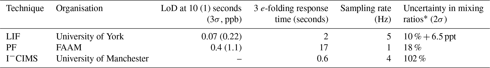
^* The uncertainty given for the I⁻CIMS is the uncertainty in the cps data since no mixing ratios were reported (see Sect. 2.3).

2.1 Laser-induced fluorescence

The University of York's laser-induced fluorescence (LIF) instrument is a custom-built system for the highly sensitive detection of SO₂, based on the system originally demonstrated by Rollins et al. (2016) and improved by Rickly et al. (2021). The fifth harmonic (216.9 nm) of an in-house built pulsed tuneable fibre-amplified semiconductor diode laser system (1084.5 nm, 3 ns pulse duration, 200 kHz repetition rate) is used to selectively excite SO₂, and the subsequent fluorescence photons are detected using a photon counting head (Hamamatsu H10682-210). The laser wavelength is tuned on and off a strong SO₂ transition peak to the $\stackrel{\mathrm{̃}}{C}$ band ($\stackrel{\mathrm{̃}}{C}{(}^{\mathrm{1}}$B${}_{\mathrm{2}})\leftarrow \stackrel{\mathrm{̃}}{X}{(}^{\mathrm{1}}$A₁)), which is tracked using a reference cell that is maintained at a constant SO₂ concentration. The difference between the number of fluorescence photons at these positions is directly proportional to the SO₂ concentration within the sample cell.

The University of York laser system differs from that described in Rickly et al. (2021) in that we use a semiconductor optical amplifier (SOA, Innolume) to pulse the continuous wave output of a distributed feedback seed laser diode (Innolume) at 200 kHz. The SOA is temperature controlled to 25 °C to ensure reproducible laser pulse generation. Other notable differences to Rollins et al. (2016) are that we use a proportional valve (Bürkert 2873) to maintain constant mass flow, and a pressure controller (Alicat PCH-100TORRA-D-MODTCPIP-A515) to maintain cell pressure.

Figure 1 Example laboratory SO₂ calibration in zero air where the LIF signal is the difference between the linearised and normalised on-line and off-line sample cell counts. The orange line shows a York regression fit to the seven data points, indicating a slope of 38.7±2.1 counts s⁻¹ mW⁻¹ ppt⁻¹, a y-intercept of 620±1700 counts s⁻¹ mW⁻¹ (both 2σ confidence), and a correlation coefficient of R²=1.0. The x error bars are dominated by the uncertainty in the SO₂ calibration standard (±5 %), but also include uncertainties in the mass flow controllers (±(0.8 % of reading + 0.2 % of full scale)) and the cell flow meter (±3 %). The y error bars (not visible) represent two standard errors of the LIF signal.

The pulse pair resolution of the photon counting head detector (20 ns) limits the available signal count rate to be equal to the repetition rate of the excitation laser, resulting in a need for a linearity correction that is important at high signal rates (Rollins et al., 2016). However, due to the combined effect of relatively low laser power (see below) and high laser repetition rate (200 kHz) in this work, the correction was only effective mainly for ship plume measurements where mixing ratios reached 140 ppb. Linearised counts are then normalised by laser power, which is measured by a phototube (Hamamatsu R6800U-01). The difference between the corrected fluorescence counts at the on-line and off-line laser wavelength positions is converted to SO₂ mixing ratio via the sensitivity factor of the system (Eq. 1), which is determined as the slope of a calibration plot using a dynamic dilution of an SO₂ standard in air. An example of a multi-point calibration from a laboratory experiment is shown in Fig. 1.

$$\begin{array}{}\text{(1)}& \left[{\mathrm{SO}}_{\mathrm{2}}\right]={\displaystyle \frac{S_{\mathrm{online}}-S_{\mathrm{offline}}}{C_{{\mathrm{SO}}_{\mathrm{2}}}}}\end{array}$$

where [SO₂] is the SO₂ mixing ratio (ppt), S_online and S_offline are the on-line and off-line linearised and normalised fluorescence counts (counts s⁻¹ mW⁻¹), and $C_{{\mathrm{SO}}_{\mathrm{2}}}$ is the experimentally determined sensitivity factor of the system to SO₂ (counts s⁻¹ mW⁻¹ ppt⁻¹).

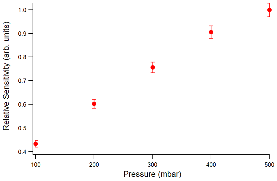
Figure 2 Relative LIF sensitivity factor over a cell pressure range of 100 to 500 mbar. The error bars are derived from the sensitivity uncertainties (Fig. 1), given to two standard errors.

Figure 2 shows how the relative sensitivity (calculated via normalising the sensitivity factor at a given pressure by that at 500 mbar) varies with cell pressure for the York LIF system. Whilst the number of SO₂ molecules per unit volume increases by a factor of 5 from 100 to 500 mbar, the sensitivity factor only increases by approximately a factor of 2 due to the increasing importance of quenching at higher pressures. During the ACRUISE-3 flights, the use of a pressure-building ram inlet allowed both the sample and reference cells to be operated at 400 ± 2 mbar for the full altitude range (between 0.07 and 3.2 km) of the campaign to maximise instrument sensitivity (Fig. 2) at the lower external pressures.

Figure 3 LIF precision (Allan deviation) of a 10 min stable ambient measurement of mean mixing ratio 75 ppt during flight C287 (orange) and a 3.5 h zero air measurement, performed recently in the laboratory with improved laser power and sensitivity (blue). Both traces are compared to the expected precision (Poisson limit). The precision (1σ) at an averaging time of 10 s for each trace is marked by the red dots (23 ppt for the orange trace, 5.4 ppt for the blue).

The ACRUISE-3 aircraft campaign was the first deployment of the York LIF instrument in the field. At the time, we were facing difficulties with lower fifth harmonic laser power (mean power of ∼ 27 µW during the campaign) compared to Rollins et al. (2016) (∼ 1 mW), using a comparable optical setup. Therefore, the 3σ LoD was determined as 70 ppt at 10 s from a stable ambient measurement of mixing ratio close to the LoD, which is shown by the orange Allan deviation trace in Fig. 3.

Table 2 Summary of the calibrations performed in both ambient air and zero air during each flight, showing the mean sensitivity ($\stackrel{\mathrm{‾}}{x}$), standard deviation of the sensitivities (σ) and the number of calibrations (N).

During the ACRUISE-3 flights, multi-point calibrations were carried out using a 5 ppm SO₂ in N₂ standard (BOC, ±5 %) added to the end of the inlet across the expected concentration range (0.5–12.5 ppb) approximately every 30 min to ensure data accuracy and to capture instrumental drift. The observed drift resulted from variations in laser linewidth caused by external temperature fluctuations within the aircraft cabin, which directly impacts instrument sensitivity. A flow rate of 2 SLPM was used, giving a 3 e-folding response time of ∼ 2 s. To assess the possible quenching effect of excited SO₂ by water vapour, or increased wall losses when sampling humid air, calibrations in both stable ambient air and dry zero air were carried out, for which these effects proved negligible as shown in Table 2. For calibrations in zero air, it was necessary to overflow the inlet, however, subsequent analysis deemed this overflow insufficient for a true zero to be measured (likely a result of pressure build-up in the inlet line from the ram inlet). Since these calibrations were performed during stable ambient mixing ratios in absence of any spikes in SO₂, such as the conditions shown in Fig. 11, the calculated sensitivities are unlikely to be affected. Hence, we justify including the calibrations in zero air in our analyses. As the sensitivities during the course of a flight largely agree within errors (Figs. S1–S3), a mean sensitivity has been calculated from both calibrations in ambient and zero air, and applied on a flight-by-flight basis. Finally, the uncertainty in the SO₂ mixing ratios were calculated from the uncertainty in the instrument sensitivity via a York regression fit to a calibration plot (Wu and Yu, 2018, Fig. 1). This gives a 2σ uncertainty of ∼ 10 % + 6.5 ppt across each flight.

Since the ACRUISE-3 campaign, improvements have been made to the York LIF system. Firstly, the conversion efficiency of the fifth harmonic generation has been improved by replacing the KTP crystal with a temperature-controlled PPLN crystal, yielding a ∼ 30-fold increase in UV laser power. In addition, the efficiency of the collection optics has also been improved by adding a lens (Edmund, #49-695) before the PMT module to focus the fluorescence into the detection head, giving a factor of ∼ 4 better sensitivity. These advancements have substantially improved the instrument's precision, as shown by the blue Allan variance trace in Fig. 3.

2.2 Pulsed fluorescence

As part of the core instrumentation on board the FAAM aircraft, a commercial Thermo Fisher Scientific model TEi-43i TLE SO₂ analyser was used to measure SO₂ during the entire ACRUISE campaign. Based on the UV pulsed fluorescence (PF) technique, it uses a broader, non-tuneable SO₂ excitation wavelength range compared to LIF and hence is more susceptible to interfering species. To minimise SO₂ fluorescence quenching by water vapour, the PF analyser is equipped with an external Nafion dryer (PermaPure Multi-strand, PD-50T-24MPR). A heated hydrocarbon kicker is used to remove interferences caused by volatile organic compounds which fluoresce at similar UV wavelengths to that of SO₂. Owing to their broad spectral features relative to SO₂, these compounds do not interfere with SO₂ mixing ratio measurements using the LIF technique, as they contribute equally to background counts at both the on-line and off-line wavelengths.

Modifications were made to the PF analyser in 2016 to improve its suitability for airborne measurements. The sample flow rate was increased from approximately 0.5 to 2 SLPM to improve the instrument response time by replacing the original TEi43i glass capillary and flow sensor with a mass flow controller (MFC3, Alicat Scientific, MCS-5SLPM-D-I-VITON). Also, a second hydrocarbon kicker was added to enhance sample flow conductance at this higher sample mass flow rate.

During the flights, the PF analyser was run at a flow rate of 2 SLPM, giving an in-flight response time (3 e-folding) of 17 s. A comparable inlet to the LIF instrument was used. In-flight single point calibrations were carried out by overflowing the instrument inlet with a 2.5 SLPM mass flow controlled calibration gas mixture of 374 ppb SO₂ in Air (BOC, ±6 %). Multi-point calibrations were also performed on the ground post-ACRUISE-3 deployment as a check of the sensitivity. To account for baseline drift, frequent (∼ 10 to 15 min interval) zero measurements were performed by passing the air sample through an external zero air scrubber cartridge filled with activated charcoal. Mean zeros are then linearly interpolated to provide a drift-corrected baseline, which is subtracted from the raw fluorescence counts, before being scaled by the detector sensitivity.

The instrument LoD (3σ) during the ACRUISE-3 deployment has been determined as 400 ppt at 10 s. Finally, the overall uncertainty in SO₂ mixing ratios has been calculated as ±18 % for a 2σ confidence interval.

2.3 Iodide chemical ionisation mass spectrometry

Matthews et al. (2023) have previously described in detail the University of Manchester (UoM) iodide ion-High Resolution-Time of Flight-Chemical Ionisation Mass Spectrometer (I⁻CIMS, Aerodyne Research, Inc) for use on the FAAM Research Aircraft. Briefly, iodide ions cluster with sample gases in the pressure-controlled ion-molecule reaction (IMR) region creating a stable adduct. The flow is then sampled through a critical orifice into the first of the four differentially pumped chambers in the CIMS, the short segmented quadrupole (SSQ), which is also independently pressure controlled. Quadrupole ion guides transmit the ions through these stages. The ions are then subsequently pulsed into the drift region of the CIMS where the arrival time is detected with a pair of microchannel plate detectors with an average mass resolution of 4000 ($m/\mathrm{\Delta }m$). The UoM I⁻CIMS operates with an IMR pressure of 72 mbar for aircraft campaigns and instrument backgrounds are taken every minute for 6 s by overflowing the inlet with ultra-high purity (UHP) nitrogen. The CIMS instrument analysis software (ARI Tofware version 3.1.0, Stark et al., 2015) was utilized to obtain high resolution, 1 Hz, time series of the compounds presented here. Mass-to-charge calibration was performed for 5 known masses; I⁻, I⁻•H₂O, I⁻•HCOOH, I${}_{\mathrm{2}}^{-}$, I${}_{\mathrm{3}}^{-}$, covering a mass range of 127 to 381 $m/z$. The mass-to-charge calibration was fitted using a square-root equation and was accurate to within an average of 1 ppm.

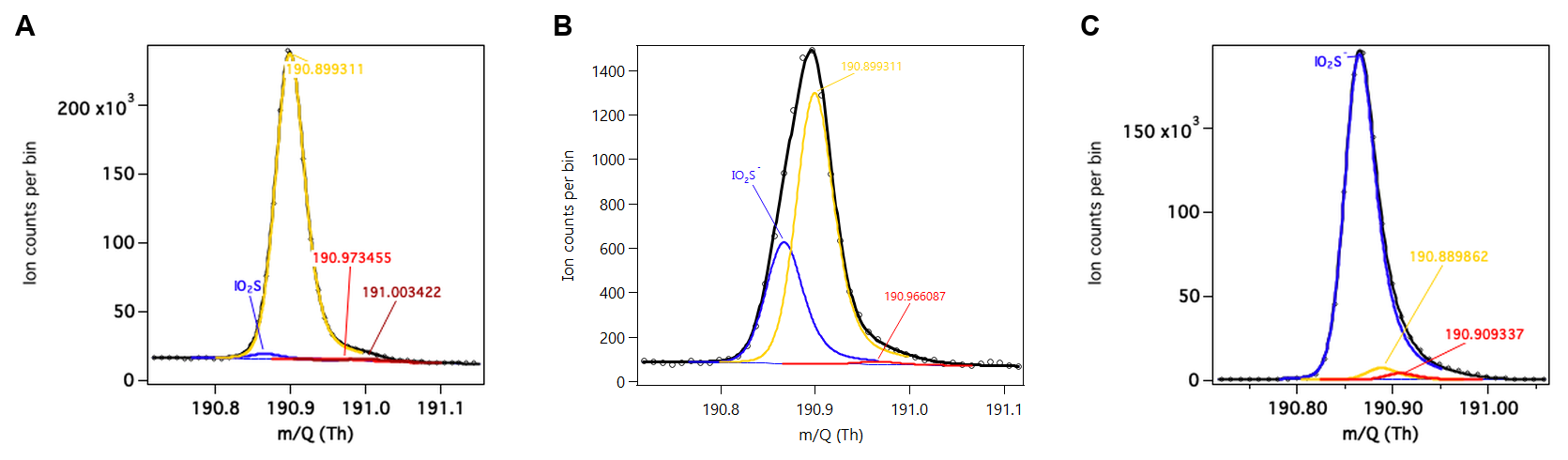
Figure 4 High resolution peak fitting at $m/z$ 191 during ambient sampling in ACRUISE-3 for (A) average mass spectrum for flight C285 (left), (B) in a ship plume (middle) and (C) calibration using a commercial standard (right).

Figure 5 Time series of the high-resolution peak fitting at $m/z$ 191 taken at 4 Hz. Peaks at ∼ 13:33 and 13:40 UTC are due to ship plumes.

I⁻CIMS detects SO₂ as a cluster with iodide at $m/z$ 190.866372. During the ACRUISE-3 campaign, the SO₂ peak is in close proximity to a larger interfering peak, likely an isotope of nitric acid, as shown in Fig. 4. The UoM I⁻CIMS has sufficient resolving power to accurately separate the overlapping peaks. Diagnostic tools in the analysis software (ARI Tofware version 3.1.0, Stark et al., 2015) have been used to estimate the uncertainties in the signal intensity fitted for SO₂ due to the mass calibration and multipeak fitting. However, despite the very accurate mass calibrations there is still an associated uncertainty of approximately 30 % for the signal intensity from an offset of 1 ppm. Additional uncertainties arise from the multipeak fitting at $m/z$ 191 and for SO₂ is an average of 97 % when measuring in ambient air (Fig. 5). This uncertainty however decreases in ship plumes as the magnitude of the SO₂ peak increases. In comparison, the uncertainty in the signal fitted for SO₂ during the offline calibration is significantly reduced and is 3 % for the multipeak fitting.

The I⁻CIMS SO₂ measurements were calibrated offline using a stable flow of SO₂ generated using a commercially sourced known concentration gas mixture (BOC, 1 ppm ± 5 % of SO₂ diluted in air) and a custom-built dynamic dilution system, which allows for a calibration gas to be diluted into a carrier gas, and in this instance, ultra-high purity (UHP) N₂ was used. The concentration of the outflow can be controlled by varying the flows of the calibrant and carrier gas, each of which are individually regulated using two MFCs (Alicat Scientific, MCS-5SLPM-D-I-VITON and MCS-500SCCM-D-I-VITON). In this case 1.2 SLPM of the outflow was delivered to the CIMS by 1$/$4” PTFE tubing and the overflow exhausted at calculated concentrations of 25, 50, 75, and 100 ppb. Additionally, the instrument's humidity dependence to the detection of SO₂ was calculated by actively adding water vapour into the IMR by passing UHP N₂ through deionised water (Fig. 6). The presence of I•H₂O⁻ clusters, which are proportional to humidity of the air as it enters the instrument, can alter the ionisation efficiency of species detected by I⁻CIMS and for SO₂ results in decreased sensitivity with increasing I•H₂O⁻ clusters (i.e. negative humidity dependence). Inconsistencies in the calibration results with measured concentrations in the field revealed an unquantifiable offset in the retrieved SO₂ data, for this reason the CIMS data will be presented in counts per second (cps) and utilised to assess the varying time response of the three instruments.

Figure 6 UoM I⁻CIMS humidity dependent sensitivity to SO₂ determined from an offline calibration using a commercial standard of SO₂. The error bars represent one standard deviation.

3 Results and discussion

This work compares airborne SO₂ measurements made by the LIF instrument, PF analyser and I⁻CIMS based on their measured time series, instrument precision and response time during the ACRUISE-3 campaign. To construct a consistent dataset from all three instruments, each time series has been averaged to 10 s (by taking the mean of each 10 s block). This averaging time was chosen as a balance between the rapid changes observed due to the direct sampling of ship plumes and the response time of the PF analyser of 17 s. The comparison is split between polluted (high SO₂) and clean (low SO₂) regions due to the different analytical requirements for measurements in these distinct environments. A map showing all three flight tracks, coloured by the LIF SO₂ mixing ratios, is shown in Fig. S4.

3.1 Polluted environments

Measurements made in polluted SO₂ marine environments include those in individual ship plumes and within shipping lanes. An example of a polluted time series comparison from flight C285 is shown in Fig. 7 which contains a series of time-matched ship plume events. Comparing the magnitude of these peaks suggests that the LIF instrument and PF analyser agree well. These conclusions are consistent with the correlation plots containing data from all three ACRUISE-3 flights. Figure 8A shows the correlation between the LIF instrument and PF analyser from 400 ppt (the PF LoD at 10 s) to the greatest plume mixing ratio of ∼ 40 ppb, and shows near-unity agreement (slope = 0.90) to within their combined uncertainties. The relationship between the CIMS data in cps and LIF SO₂ mixing ratios also displays a linear correlation (Fig. 8B) but with a poorer fit. Due to the challenges in calibrating the CIMS, described above, the gradient of this plot has been used to estimate CIMS SO₂ mixing ratios for comparison of response time and noise distributions across the three SO₂ measurement techniques.

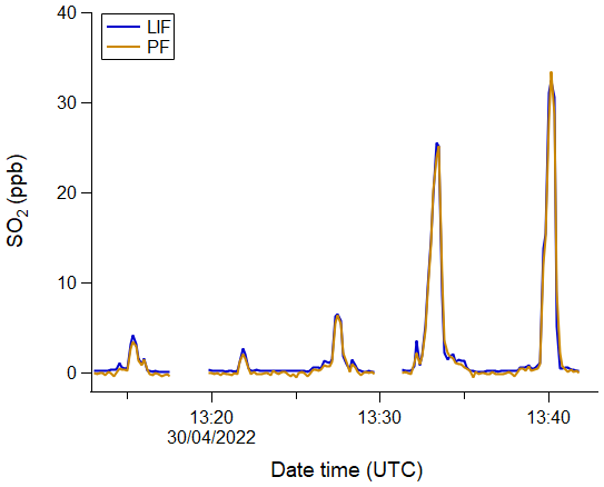
Figure 7 Time series of 10 s averaged, time matched data during flight C285, comparing LIF and PF SO₂ measurements.

Figure 8 Correlation of the 10 s averaged, time matched data for all three ACRUISE-3 flights. (A) Correlation between the PF and LIF SO₂ mixing ratios, excluding points below the instrument's LoD. (B) Correlation between the I⁻CIMS in cps and LIF SO₂ mixing ratios. The coloured dashed lines represent the ordinary least squares (OLS) regression fit and the solid black line represents the 1:1 ratio (for the mixing ratio comparison only). Gradient and intercept uncertainties have been given to a 2σ confidence interval.

A comparison of response time can be made from the time series of a single ship plume peak in Fig. 9, recorded at 5, 1 and 4 Hz for the LIF instrument, PF analyser and I⁻CIMS respectively. To remove the lag time as a result of different inlet lengths, the peaks have been time-matched by the increase in SO₂ mixing ratios upon intersecting a ship plume. Figure 9 shows the SO₂ mixing ratios recorded by the I⁻CIMS fall to out-of-plume levels the quickest and its time series displays the greatest structure. This is evident in the faster I⁻CIMS response time of 0.6 s (3 e-folding) compared to the LIF system of 2 s and the PF analyser of 17 s. The LIF signal exhibits similar structure to the I⁻CIMS data, however, the slower gas flush rate means the features are smoothed, and the LIF signal takes longer than the I⁻CIMS to return to background levels. Further improvements to the LIF system have increased its true measurement rate to 10 Hz. The comparatively slow response time of the PF analyser results in it being unable to resolve the plume structure, and shows a significant delay in returning to background levels.

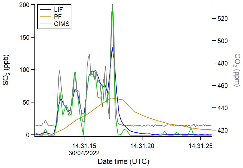
Figure 9 Time series comparing instrument response time, matched by the increasing SO₂ mixing ratio due to measurement of a ship plume during flight C285. The LIF data is presented at 5 Hz, the PF at 1 Hz, the I⁻CIMS at 4 Hz and the CO₂ data at 10 Hz. To note, I⁻CIMS SO₂ mixing ratios have been estimated based on the gradient of the fit to the LIF data (Fig. 8B).

Plume sampling can be used to quantify emissions ratios, and the ratio of SO₂:CO₂ can be used to calculate ship sulfur fuel content for applications in compliance monitoring (Beecken et al., 2014; Berg et al., 2012; Kattner et al., 2015; Lack et al., 2011; Lee et al., 2025; Yu et al., 2020). Average emissions ratios can be derived via two methods for a ship plume event: (a) the integration method where the area under the peak and above the baseline is calculated (Beecken et al., 2014; Kattner et al., 2015; Lack et al., 2011; Lee et al., 2025; Yang et al., 2016), and (b) the regression method where the slope of a correlation plot is taken (Aliabadi et al., 2016). The regression method is a useful approach as it removes the necessity to subtract the background concentrations (Wilde et al., 2024). However, it is a less popular approach, especially for in situ airborne sampling, since it relies on sufficient data points for a statistically valid regression analysis and a similar plume structure between the two species, as shown by the SO₂ I⁻CIMS and CO₂ trace in Fig. 9. Hence, this requires fast response time instrumentation for aircraft measurements of plume transects as the plume duration can be extremely short. On the other hand, the integration method provides a response time-independent way of reliably analysing these short duration plume events.

Figure 10 Regression analysis to calculate the SO₂:CO₂ emission ratio (gradient of OLS fit) for the ship plume during flight C285. Gradient uncertainties have been given to a 2σ confidence interval.

This work makes use of the fast response time of the I⁻CIMS (to achieve fine plume structure) and the accuracy of the LIF technique to compare the integration and regression methods. Therefore, I⁻CIMS SO₂ mixing ratios have been estimated based on the gradient of the fit to the LIF data (Fig. 8B). In the integration method, background concentrations have been determined using an exponentially weighted moving average, and peak areas have been calculated relative to this baseline using a trapezoidal approximation. For the plume in Fig. 9, the corresponding regression analysis is shown in Fig. 10 and the results of this ship plume event, as well as three others, are shown in Table 3. Plots for the remaining three plumes are given in Figs. S5–S7. To note, due to the much slower response time of the PF technique, an emission ratio via the regression method could not be calculated.

Table 3 Comparison of integration and regression methods for calculating SO₂:CO₂ emission ratios of four ship plumes during different flights. The LIF SO₂, I⁻CIMS SO₂ and CO₂ data have been sampled to 4 Hz, however, the PF SO₂ data is at 1 Hz. Emission ratio uncertainties have been given to a 2σ confidence interval. The corresponding sulfur fuel content (SFC) has been calculated via Eq. (2) and is given in brackets after each emission ratio. SFC uncertainties include an estimated 6 % error to account for the emission of sulfur as sulfate.

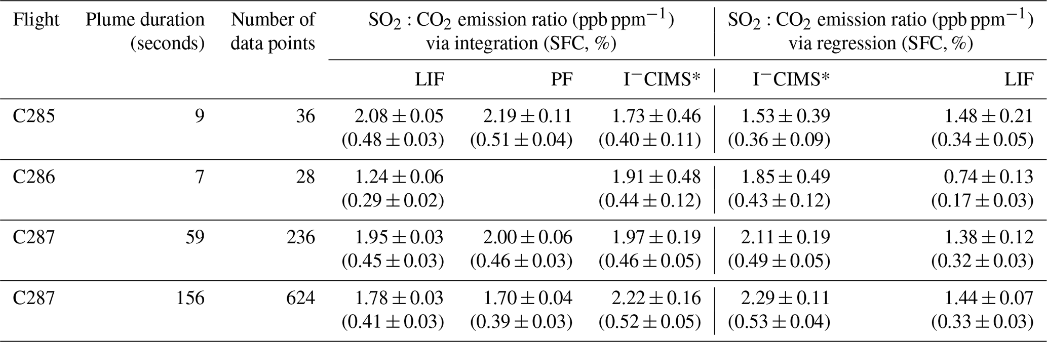
^* I⁻CIMS SO₂ mixing ratios have been estimated based on the gradient of the fit to the LIF data (Fig. 8B).

A check of the compliance of the sampled ships to the IMO2020 regulation (0.5 % sulfur fuel content in international waters) can be made through calculation of the sulfur fuel content (SFC) from the emission factors. Assuming that 87 % of ship fuel by mass is carbon, the SFC mass percent is related to the emission ratio via the following equation (Kattner et al., 2015):

$$\begin{array}{}\text{(2)}& \mathrm{SFC}\left[\mathit{\%}\right]={\displaystyle \frac{{\mathrm{SO}}_{\mathrm{2}}\left[\mathrm{ppb}\right]}{{\mathrm{CO}}_{\mathrm{2}}\left[\mathrm{ppm}\right]}}\times \mathrm{0.232}\left[\mathit{\%}\right]\end{array}$$

where the SO₂:CO₂ ratio is the emission ratio, calculated above, and 0.232 is the mass conversion factor for fuel content. Equation (2) also assumes that all sulfur is emitted as SO₂ and all carbon as CO₂. The latter of these assumptions is deemed a reasonable estimate since little to no CO was measured during the ACRUISE-3 campaign, suggesting a complete combustion pathway. However, it is known that not all sulfur is released as SO₂ – some is directly emitted as sulfate, SO${}_{\mathrm{4}}^{\mathrm{2}-}$. The amount of SO${}_{\mathrm{4}}^{\mathrm{2}-}$ released has been shown to correlate with the SFC (Yu et al., 2020) and it also increases with plume aging. Since the calculation of plume age is beyond the scope of this paper, the SFC is not corrected for sulfate (which is estimated as 6 % for a plume age of max. 15 min (Yu et al., 2020)), and this 6 % discrepancy has been included in the uncertainty. The corresponding SFCs of the sampled ships are given in brackets after each emission ratio in Table 3, which shows they are all compliant to the IMO2020 regulation.

As shown in Table 3, the accuracy of the regression method for calculating emission ratios is dependent on the response time of the instrument. The I⁻CIMS has a response time closer to that of the CO₂ measurements and hence gives emission ratios that are in greater agreement to those calculated via the integration method. The consistently lower regression emission ratios derived from the LIF data are likely due to the smoothing effect as a result of a longer response time compared to the I⁻CIMS. However, the I⁻CIMS is limited by its large uncertainty and its greater R² values suggest that a single factor correction is unable to capture any variability associated with the interference. Therefore, improvements to the LIF system's response time will make it the more desirable instrument for calculating emission ratios via the regression method.

3.2 Clean environments

In order to understand the role of sulfur in controlling particle formation in remote regions, and thus their direct and indirect climate impacts, measurements of SO₂ need to be made with sufficient sensitivity and precision to provide observations at a time resolution capable of constraining on our understanding of key processes. A comparison of precision and noise distribution has been made for the three instruments from low SO₂ mixing ratios measured in clean marine environments, outside of shipping lanes. Figure 11A shows an example time series comparison of clean SO₂ measurements from flight C286. Two observations can be made from this time series comparison which are more evident in the corresponding histogram plot in Fig. 11B: (1) SO₂ is above the LIF instrument's LoD, unlike the PF analyser and I⁻CIMS and (2) the distribution of the LIF signal is much narrower than the PF analyser and I⁻CIMS signals, given their standard deviations of 0.044, 0.14 and 0.27 ppb respectively. For exploring statement (1), it is necessary to consider the 3σ LoDs of the three instruments during the flight at the same averaging time as the time series and each other (10 s). These are 0.07 and 0.4 ppb for the LIF instrument and PF analyser respectively at 10 s, and even higher for the I⁻CIMS. Comparing the mean mixing ratios measured by the LIF instrument, PF analyser and I⁻CIMS of 0.18, −0.094 and 0.050 ppb respectively, it is evident that the LIF system is sensitive enough to capture these low mixing ratios. This is not the case for the PF analyser and I⁻CIMS and therefore their observed distributions are indistinguishable from a measurement of zero.

Figure 11 Time series (A) and histogram (B) of 10 s averaged, time matched data during flight C286, comparing the LIF instrument, PF analyser and I⁻CIMS SO₂ measurements. The distributions are divided into 10 bins for each instrument and hence the bin widths are scaled accordingly.

The 15 min time period in Fig. 11A has been chosen as the ambient measurements are relatively stable and hence useful for comparing instrumental noise in flight via the width of the distributions in Fig. 11B. We have assumed a well-mixed atmosphere and that the LIF signal distribution is determined predominantly by instrumental noise (evidenced by Fig. S8). Therefore, as ambient variability is present but minimal, the LIF signal distribution is an upper limit assessment of its precision. We conclude that the noise distribution for the LIF instrument is significantly narrower than the PF analyser and I⁻CIMS, making it a powerful tool for capturing SO₂ mixing ratios in remote marine environments at a range of altitudes. Figure S9 shows an altitude plot of LIF SO₂ mixing ratios averaged across each 100 m bin width for all three ACRUISE-3 flights. This data is compared to SO₂ mixing ratios measured by the LIF instrument during the seventh aircraft campaign of The North Atlantic Climate System Integrated Study (ACSIS-7) (Archibald et al., 2025), which sampled clean remote marine air over the North Atlantic during 5–9 May 2022. It is evident that the marine environment sampled during ACSIS-7 was cleaner at the sea surface, likely reflecting the reduced influence of ship emissions compared to ACRUISE-3. SO₂ mixing ratios, however, become increasingly comparable to those measured during ACRUISE-3 at higher altitudes and display a similar decreasing trend with altitude up to 2000 m due to vertical mixing and diffusion from marine SO₂ sources. The ACSIS-7 profile exhibits a notable mixing ratio inversion at 2000 m, coincident with the marine boundary layer height.

While reported observations of SO₂ altitude profiles over the ocean are scarce, relevant comparisons can be drawn from measurements in the Atlantic between 30N–54N during the ATom campaigns (Bian et al., 2024). Considering differences in sampling strategies, time of year and location etc., the ATom profiles are consistent with our observations, showing SO₂ mixing ratios of a similar order of magnitude, albeit slightly lower, and a comparable decreasing trend with altitude (up to 3.8 km).

4 Conclusions

Three SO₂ instruments were involved in an intercomparison experiment on board the U.K. FAAM research aircraft: LIF, PF and I⁻CIMS. A range of SO₂ concentrations were measured, from <70 ppt in clean marine environments up to 40 ppb in ship-polluted environments (at 10 s averaging), west of the English Channel over international waters. In polluted environments, SO₂ measurements made by the LIF instrument and PF analyser agreed within the errors of the instruments. However, the LIF and I⁻CIMS measurements were found to disagree by a constant factor. This work has also allowed a comparison of SO₂:CO₂ emission ratio calculation methods (integration versus regression), and the regression method has proved to be in greater agreement to the integration method when using fast time response instrumentation. In clean environments, the ambient mixing ratios are below the LoDs of the PF and I⁻CIMS instruments, and therefore the LIF system is the only instrument in this study able to detect SO₂ mixing ratios between 70 and 400 ppt. From this intercomparison, we conclude that for measurements of low SO₂ concentrations requiring high sensitivity and low noise, such as those in remote marine environments, LIF is a powerful technique. While I⁻CIMS has demonstrated a response time approximately three times faster than LIF, making it more suitable for aircraft measurements, its sensitivity to SO₂ is limited and for the instrument used in this study, has unresolved issues surrounding accurate quantification. Ongoing improvements to the LIF instrument have improved its LoD to 16.2 ppt at 10 s (3σ) and increased its flush rate towards flux-scale response times (>5 Hz), enabling both fast and accurate measurements of SO₂. All three techniques are valuable for improving our understanding of atmospheric SO₂, but application dependent. The LIF technique is becoming more crucial both today and in the future, as more stringent emission reductions, such as the IMO2020 regulation, lead to cleaner SO₂ environments.