Recalibration of low-cost O₃ and PM_2.5 sensors: linking practices to recent air sensor test protocols

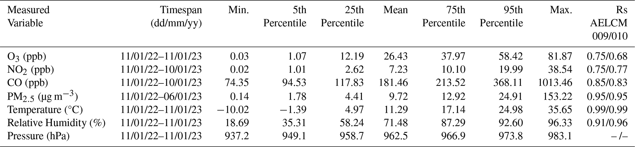
The appropriate period of collocation of a low-cost air sensor (LCS) with reference measurements is often unknown. Previous LCS studies have shown that due to sensor ageing and seasonality of environmental interferences periodical sensor calibration needs to be performed to guarantee sufficient data quality. While the limitations are well-established it is still unclear how often a recalibration of a sensor needs to be carried out. In this study, we demonstrate how widely used air sensors (OX-B431 and SPS30) for the relevant air pollutants ozone (O₃) and fine particulate matter (PM_2.5) by two manufacturers (Alphasense and Sensirion) should be recalibrated for real-world monitoring applications. Sensor calibration functions were built using Multiple Linear Regression, Ridge Regression, Random Forest and Extreme Gradient Boosting. We use multiple novel test protocols for air sensors provided by the United States Environmental Protection Agency and the European Committee for Standardization for evaluative guidance and to identify possible applications for OX-B431 and SPS30 sensors. We conducted a yearlong collocation campaign at an urban background air and climate monitoring station next to the University Hospital Augsburg, Germany. LCSs were exposed to a wide range of environmental conditions, with air temperatures between −10 and 36 °C, relative air humidity between 19 % and 96 % and air pressure between 937 and 983 hPa. The ambient concentration ranges for O₃ and PM_2.5 were up to 82 ppb and 153 µg m⁻³, respectively. For the baseline single training of 5 months, the calibrated O₃ and PM_2.5 sensors were able to reflect the hourly reference data well during the training (R²: O₃ = 0.92–1.00; PM_2.5 = 0.93–0.97) and the following test period (R²: O₃ = 0.93–0.98; PM_2.5 = 0.84–0.93). Additionally, the sensor errors were generally acceptable during the training (RMSE: O₃ = 0.80–4.35 ppb; PM_2.5 = 1.45–2.51 µg m⁻³) and the following test period (RMSE: O₃ = 3.62–5.84 ppb; PM_2.5 = 2.04–3.02 µg m⁻³). We investigated different recalibration cycles using a pairwise calibration strategy, which is an uncommon method for recurrent LCS calibration. Our results indicate that a regular in-season recalibration is required to obtain the highest quantitative validity and broadest range of applications (indicative and non-regulatory supplemental measurements) for the analysed LCSs. Monthly recalibrations are observed to be the most suitable approach. The measurement uncertainties of the calibrated O₃ LCSs and PM_2.5 LCSs were able to meet the data quality objective for indicative measurements for different calibration models. In-season recalibration, rather than reliance on a single pre-deployment calibration, should be adopted by end-user communities. This approach is required for certain real-world applications to be performed reliably by LCSs and to achieve sufficient information content.

1 Introduction

Low-cost sensors (LCSs) form an interesting approach for monitoring air pollution in a denser network than currently available due to the cost of regular fixed measurement stations. Basically, they are smaller, consume less power, are cheaper and therefore more accessible than regular monitoring devices for air pollution (Lewis et al., 2018; Li et al., 2020; Peltier et al., 2021; Schäfer et al., 2021; Narayana et al., 2022). This underlines why there is an interest among researchers, governments, businesses and individuals in using LCSs for air quality monitoring in different settings, e.g. citizen science, mobile and stationary monitoring (in for instance urban or remote locations), urban planning, personal exposure science or education (Williams et al., 2019; Mahajan and Kumar, 2020; Mahajan et al., 2020; Peltier et al., 2021; Okure et al., 2022; Hassani et al., 2023; Malings et al., 2024). This interest has led researchers to develop their own custom-built air quality monitoring systems equipped with LCSs (Mueller et al., 2017; Cross et al., 2017; Gäbel et al., 2022), which can be more widely used in the aforementioned settings.

Nevertheless, those sensors also have their disadvantages. At present they do not fulfill the stringent requirements for regulatory measurements provided by high-quality air pollutant monitoring systems used by governments to monitor the exceedance of health-relevant thresholds for air pollutants like ozone (O₃), nitrogen oxides (NO_x), particulate matter (PM_2.5, PM₁₀), carbon monoxide (CO), and sulfur dioxide (SO₂) (Castell et al., 2017; Wesseling et al., 2019; Schäfer et al., 2021). Major issues with LCSs are their short operating life, lack of long-term stability due to sensor ageing, interferences, cross-sensitivities and the need for calibration functions to adjust LCS bias and transform LCS output into meaningful units (Lewis et al., 2018; Peltier et al., 2021; Concas et al., 2021; Carotenuto et al., 2023). Hence reference measurements are needed. The inter-sensor unit variability of LCSs is another issue, where a calibration function derived through training data for a LCS is usually not by default transferable. LCS data of a unit can be quite unique, when compared to data of another unit of the same model (Moltchanov et al., 2015; Gäbel et al., 2022; Bittner et al., 2022). However, good-performing sensors can act as devices for non-regulatory supplemental and informational monitoring (NSIM) applications (Duvall et al., 2021a, b). LCS performance must be assessed, and data quality control processes must be developed to establish confidence in LCS data (Malings et al., 2024). Consequently, the question of whether a selected air sensor is a good fit for its planned purpose must be answered (Diez et al., 2022). Snyder et al. (2013) summarized the essence of the problem in one sentence: “Data of poor or unknown quality is less useful than no data since it can lead to wrong decisions”.

Uniform evaluation and comparison methods for LCSs are incentivized by a growing market, which offers a greater supply of more refined LCSs. The lack of standardized procedures was recognized in the literature in recent years (Rai et al., 2017; Karagulian et al., 2019; Williams et al., 2019; Duvall et al., 2021a). Therefore, there is an initiative by multiple organizations to develop test programs and test protocols like the Environmental Protection Agency (EPA) of the United States or the European Committee for Standardization (CEN) (Duvall et al., 2021a, b; CEN/TS 17660-1:2021, 2021; CEN/TS 17660-2:2024, 2024). The development of test programs by organizations, which are also recognized by governmental bodies, is an important achievement. They create a foundational framework to collect comparable harmonized metrics to assess LCS data quality. Thus, they help to develop a standardized quality assessment to ultimately justify the use of LCSs in defined areas of interest in air pollution monitoring. Hence it is a further step for establishing reliable low-cost air quality networks within the regulatory monitoring system for air quality worldwide. Using target metrics and sensor (tier) classifications from these test programs to better understand air sensor performance and their potential role within the broader air quality information system is not yet common practice in studies evaluating LCSs across different settings. The current air quality information system is defined by reference-grade monitoring, satellite monitoring and air quality modeling.

One important aspect is recalibrations of LCSs after their initial (on-site) calibration using reference monitors, which is an important point in network management to guarantee long-term data quality (Concas et al., 2021; Carotenuto et al., 2023). However, most of the recent studies doing long-term field campaigns using LCS networks for air quality monitoring show in their methods no recalibration strategy to mitigate the effect of sensor ageing and thus to enhance the LCS measurement output under a quantitative point of view (Jayaratne et al., 2020; Petäjä et al., 2021; Mohd Nadzir et al., 2021; Bílek et al., 2021; Raheja et al., 2022; Kim et al., 2022; Collier-Oxandale et al., 2022; Okure et al., 2022; Connolly et al., 2022). For instance, the official warranted operating lifespan of the commonly used electrochemical (EC) LCS NO2-B43F by the company Alphasense is only 2 years (Alphasense, 2024a) or even lower according to Li et al. (2021). They investigated the long-term degradation of EC Alphasense NO₂ sensors in the field and found evidence that those sensors could already malfunction after 200 d. Furthermore Kim et al. (2022) calibrated Alphasense NO₂ sensors based on a 6-month collocation using regulatory monitoring devices at a rural traffic site. 1.5 years later Kim et al. (2022) did a second collocation experiment with the same sensors at the same site using their original calibration functions from the first collocation. They found a significant deterioration in sensor performance during the second collocation. It was also discussed that due to time-varying effects of environmental interferences (e.g. air temperature, relative humidity), sensor performance can vary with season (Ratingen et al., 2021; Peters et al., 2022). For these reasons, LCS recalibration intervals of less than 1 year and methods for regular LCS data quality checks using regulatory monitoring devices need to be explored whether those sensor devices are supposed to be used in lengthy measurement campaigns to assess air quality. At present, it remains unclear how regularly LCSs need to be recalibrated. The number of publications investigating varying calibration periods is not exhaustive due to the lack of long-term collocation experiments in the available literature. Generally, studies which investigate varying recalibration periods look only at a specific air pollutant sensor targeting one air pollutant. They do not apply state-of-the-art test programs for LCSs to categorize their results in frameworks provided by organizations, which are officially recognized by governmental authorities. In this context, this study presents a concept for recurrent LCS calibration for real-world applications by using various performance metrics based on multiple novel test protocols.

We investigated different recalibration cycles for commonly used LCSs for NO₂, O₃, CO and PM_2.5 using metrics and target values provided by EPA and CEN (Duvall et al., 2021a, b; CEN/TS 17660-1:2021, 2021; CEN/TS 17660-2:2024, 2024). We conducted the investigation during a 1-year on-site collocation experiment in the city of Augsburg, Germany.

This work is organized as follows. The section about materials and methods describes the infrastructure used for the collocation experiment and the methodology behind our sensor calibration strategy and its evaluation. The “Results and discussion” section focuses on the environmental conditions and pollution concentrations observed during the collocation experiment, the performance of the introduced LCS calibration models under different recalibration cycles and the potential implications of our findings for LCS networks. The concluding remarks can be found in the last section.

2 Materials and methods

An in-depth investigation was done for LCSs measuring O₃ and PM_2.5. Due to test site limitations affecting the ability to classify LCSs for NO₂ and CO according to CEN, LCSs for these air substances could only be classified using the EPA test protocol for gas sensors. Two Atmospheric Exposure Low-Cost Monitoring (AELCM) boxes were mounted next to the Atmospheric Exposure Monitoring Station (AEMS) for air substances and meteorological variables. The boxes included the LCSs for the mentioned air pollutants while the latter provided the reference measurements in the present study. The AEMS is operated by the Chair for Regional Climate Change and Health at the University of Augsburg.

2.1 AELCM sensor box

Two advanced AELCM sensor boxes, denoted as AELCM009 and AELCM010, were used. The custom-built devices were developed by the Chair for Regional Climate Change and Health at the University of Augsburg. A detailed description and performance check of the first version of the low-cost measurement unit can be found in our previous study (Gäbel et al., 2022). The upgraded AELCM units measured air quality and meteorological parameters, namely O₃ (Alphasense OX-B431), NO₂ (Alphasense NO2-B43F), CO (Alphasense CO-B4), PM_2.5 (Sensirion AG SPS30) as well as humidity and air temperature (Bosch BME280) (Bosch Sensortec, 2015; Sensirion, 2020; Alphasense, 2024a, b, c). In this study the air pollution sensors were denoted as AS-B431, AS-B43F, AS-B4 and SAG-SPS30. Table 1 summarizes the specifications of the air sensors, with technical details taken from the manufacturers' official data sheets (Sensirion, 2020; Alphasense, 2024a, b, c). The upgrade of the AELCM boxes with respect to the previous study was related to the switch to EC gas sensors from Alphasense, which exclusively measured the earlier mentioned gaseous air substances. The upgrades also involved the increase of the sampling frequency for each AELCM sensor from 10 s to every 4 s. A code rework on the Arduino microcontroller board made it possible to measure on a higher temporal resolution.

Table 1 Overview of the specifications of air sensors that can be used in the AELCM unit.

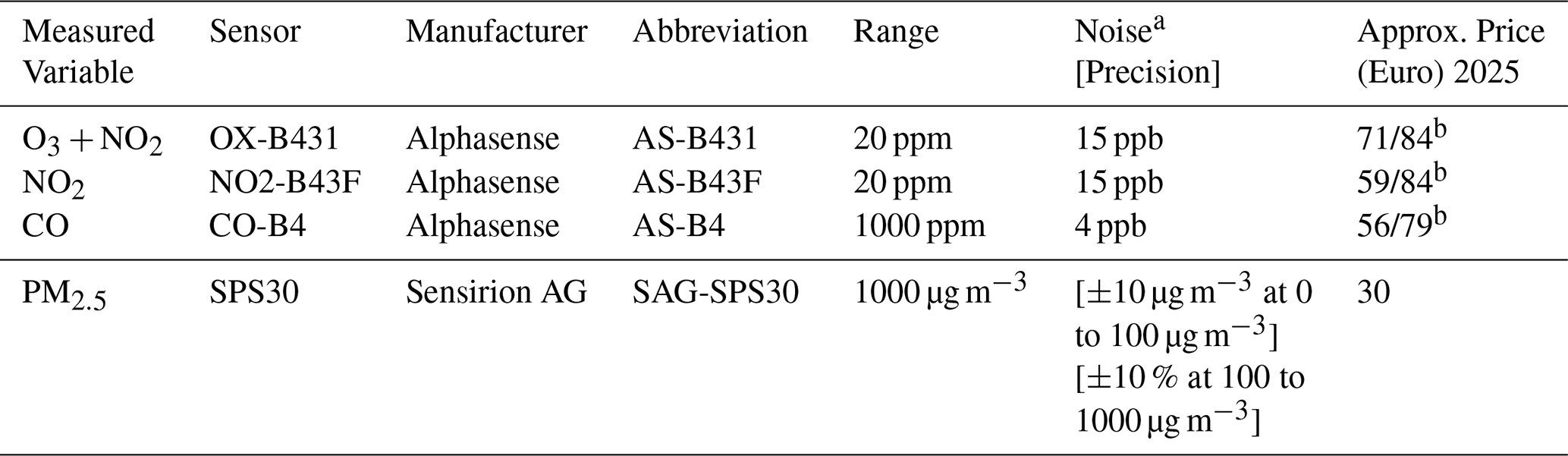
^a Tested with Alphasense ISB low noise circuit: ±2 standard deviations (ppb equivalent). ^b Additional cost for the Individual Sensor Board (ISB) low noise circuit for B sensors.

There were multiple reasons for the use of Alphasense sensors. In our earlier work (Gäbel et al., 2022), we investigated the digital gas sensors DGS-NO2 and DGS-CO from SPEC Sensors, based on EC gas sensor technology, as well as the MiCS-2714 (NO₂) and MiCS-4514 (CO) sensors from SGX Sensortech, based on metal oxide semiconductor (MOS) technology. Our results showed that these air sensors exhibited no satisfactory capability to capture the observed concentrations at a measurement station, according to the coefficient of determination after sensor calibration (R²: 0.15–0.66). Therefore, we applied alternative LCSs to capture NO₂ and CO. Overall, the SPEC DGS-O3 units performed satisfactorily (R²: 0.71–0.95) but showed high inter-sensor unit variability. For the calibrated MQ131 sensor outputs moderate to high R² were determined (R²: 0.71–0.83). In contrast, the raw MQ131 sensor outputs showed generally poor correlation with the O₃ reference measurements. We concluded that EC gas sensor technology is suitable for detecting O₃ in an urban background environment, whereas MOS technology showed limited capability in the case of Winsen's MQ131 sensor. Alphasense EC gas sensors are the most used and evaluated LCSs for measuring O₃, NO₂ and CO (Karagulian et al., 2019; Kang et al., 2022) and offer a good price-to-quality ratio (see Table 1). Kang et al. (2022) reported median R² values of 0.70, 0.68 and 0.82 for these pollutants, respectively. The values were derived by Kang et al. (2022) from studies that used Alphasense EC sensors in outdoor settings in conjunction with reference instruments. In our evaluation at an urban background station (Gäbel et al., 2022), the SAG-SPS30 particulate matter (PM) sensor showed high correlative performance for calibrated data (R²: 0.90–0.94). Also, other outdoor studies showed satisfactory results for the SAG-SPS30 and its measurement of PM_2.5 (R²: 0.72–0.87) (Vogt et al., 2021; Roberts et al., 2022; Shittu et al., 2025).

2.2 Collocation with AEMS

The AELCM units were mounted on a fence right next to the AEMS, as shown in Fig. 1. The AEMS is a high-quality air and climate measurement station located next to the University Hospital Augsburg in Germany (48°23.04^′ N, 10°50.53^′ E). The station can be classified as an urban background station. Federal roads are in the south and east, respectively 850 and 1200 m located away from the station. A highway road is 3600 m located away in the North. Industrial areas relative to the station location are located further away, in the south-east and the north-east of Augsburg. Regular station measurements of varying concentrations of CO, NO₂ and PM_2.5 due to local traffic and local industry depend highly on circulation patterns favouring an air flow from those sources towards the city as well as on the day and daytime, where factors like commuting play an important role.

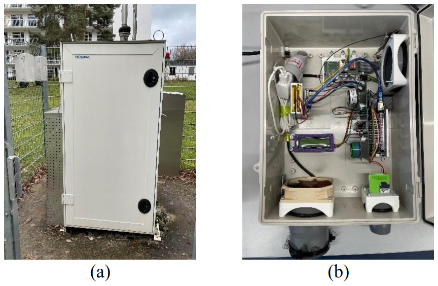
Figure 1 Photographs of the AEMS and AELCM units (AELCM009 and AELCM010), which are mounted on the fence next to the AEMS: (a) the stationary air and climate measurement station of the Chair for Regional Climate Change and Health, Faculty of Medicine, University of Augsburg; and (b) the housing and interior view of the engineered AELCM units.

The regulatory-grade air measurement instruments are from the company HORIBA. Reference measurements of O₃, NO₂, CO and PM_2.5 were conducted using the instruments APOA-370, APNA-370, APMA-370 and APDA-372, in that order. The HORIBA instruments for gaseous air pollutants are also used by the Bavarian Environment Agency for official air pollution monitoring in Bavaria (Bayerisches Landesamt für Umwelt, 2019). The weather station WS600-UMB mounted to the station provided measurements for meteorological variables. Further details about the AEMS can be found in the study of Gäbel et al. (2022).

The collocation took place from January 2022 until January 2023. The model training period for the LCSs was between 11 January 2022 till 10 June 2022. The testing period for the LCS recalibration experiment started at 10 June 2022. The experiment ended between 6 and 11 January 2023 depending on the LCS. The end is individual for each LCS model unit, because of individual missing values in the reference measurements for each air pollutant. The aim of the collocation was the assessment of the benefit of regular recalibrations against single calibration. The latter used solely the above-mentioned training period for model training. Performance metrics and their recommended target values given by novel test programs and test protocols by EPA and CEN were used to assess the influence of a recalibration procedure on LCS performance and to identify possible real-world applications for the investigated LCSs (Duvall et al., 2021a, b; CEN/TS 17660-1:2021, 2021; CEN/TS 17660-2:2024, 2024).

2.3 Data treatment

The collocation experiment involving AELCM009 and AELCM010 started initially on 10 January 2022. The used LCSs have a stabilization phase after being powered on. Only after this stabilization phase are the LCSs eligible for measurements of a target pollutant (Gäbel et al., 2022). The stabilization phase observed in the LCS measurement outputs was shorter than one day. The first 24 h of all LCS data were thus removed and not included in this study. The AS-B431 is an LCS which measures O₃ and NO₂ (Alphasense, 2024b). For the correct measurement of ambient O₃ using an AS-B431 unit, data of a LCS measuring NO₂ is required for the O₃ calibration model. For this purpose, we used an AS-B43F unit. The modelled calibration functions for the estimation of O₃ included by default the LCS output of both Alphasense sensor units. The Alphasense sensors provided voltages as measurement outputs by default. Like Bigi et al. (2018), we calculated the net voltage of every Alphasense sensor derived from the difference between the working and auxiliary electrodes. The calculated net voltages became an input for the modelled calibration functions next to the meteorological variables air temperature and relative humidity, which affect the LCS output as environmental interferences.

The system time of the AELCM units (UTC) was adjusted to the system time of the AEMS (CET). Raw LCS and AEMS reference measurements were aggregated to hourly means for LCS calibration. This resulted in calibrated hourly values of gas and PM sensors. Calibrated PM_2.5 sensor measurements were aggregated to daily means. Hourly means of gas sensor data and daily means of PM sensor data were required for the performance evaluation of LCSs according to the technical specifications (TSs) developed by CEN (CEN/TS 17660-1:2021, 2021; CEN/TS 17660-2:2024, 2024) and the test protocols developed by EPA (Duvall et al., 2021a, b). As a result, PM_2.5 measurements provided by the AEMS were also aggregated to daily means for evaluation. The missing values in the air pollution reference data were caused by regular maintenance, device malfunctions or due to power grid tests at the University Hospital. The missing values in the meteorological data were due to device malfunctions of the weather station. The LCS measurement data for each AELCM unit was nearly complete, with very few missing values, similar to the data in Gäbel et al. (2022). 100 % and at least 80 % of the data had to be available for the hourly aggregation of reference measurements of gaseous air pollutants and meteorological variables, respectively. For the calculation of the key performance metric in the TS by CEN (CEN/TS 17660-2:2024, 2024), the minimum data capture of the SAG-SPS30 was set to 90 %. Therefore, the daily means of PM_2.5 resulting from reference and LCS data were only valid if at least 90 % of the hourly averages were available within a 24 h period. Note that the data completeness criterion is less strict in the PM sensor test protocol by EPA. There, the daily mean PM_2.5 concentration is calculated on at least 75 % of hourly averages within a 24 h period (Duvall et al., 2021a). The SAG-SPS30 for the measurement of PM provides outputs in mass concentrations by default.

For gaseous air constituents the devices in the AEMS and the model-calibrated LCS devices provided measurements in the unit parts per billion (ppb). Hence for the calculation of mass concentrations the hourly aggregated meteorological measurements of the integrated weather station of the AEMS were used. Mass concentrations were needed for the performance evaluation of ambient air quality sensors for gaseous pollutants following the TS developed by CEN (CEN/TS 17660-1:2021, 2021). We solely used low-cost meteorological data from the Bosch BME280 sensors as input for the calibration models (Sect. 2.4). To calculate mass concentrations from the output of the calibration models we did not rely on BME280 meteorological data but used the weather station data. The former are highly biased due to solar radiation. The bias stems from solar heating of the AELCM units, which could not be mitigated by the integrated fan. The fan causes an exchange of air between the inside and outside yet does not reduce the heating effect. It is planned to equip the AELCM units with radiation shields in the future to reduce the effect of solar radiation on the low-cost meteorological measurements.

2.4 LCS calibration and model tuning

We built and evaluated four regression models (calibration models) for each LCS to estimate air pollution levels based on their data output (hourly means), accounting for environmental influences on sensor output and reference measurements (AEMS). The regression models were Multiple Linear Regression (MLR), Ridge Regression (RR), Random Forest (RF) and Extreme Gradient Boosting (XGB). Moving forward we will call these calibration models. Every calibration model consisted of a target variable to be predicted, and features used for prediction. As the target we defined the ambient air pollutant concentration of a specific air substance (AEMS${}_{{\mathrm{O}}_{\mathrm{3}}}$, AEMS${}_{{\mathrm{NO}}_{\mathrm{2}}}$, AEMS_CO, AEMS_PM2.5). As features used for prediction, we used the raw LCS output. The LCS output can be classified into the net voltages measured by each Alphasense sensor (V_OX_10, V_OX_09, $V_{{\mathrm{NO}}_{\mathrm{2}}}$_10, $V_{{\mathrm{NO}}_{\mathrm{2}}}$_09, V_CO_10, V_CO_09), the mass concentrations measured by each Sensirion PM sensor (SPS30_10, SPS30_09) and the air temperatures (T_10, T_09) and relative humidities (RH_10, RH_09) provided by each BME280.

Table 2 Model variables for the development of the calibration functions based on MLR, RR, RF and XGB.

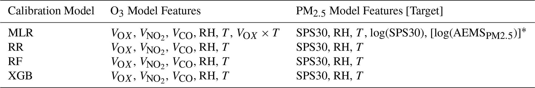
^∗ This target is shown because it is transformed in the MLR calibration model configuration.

We chose MLR models because MLR is still the most common basic approach in the literature to develop calibration models for LCSs (Karagulian et al., 2019). In this paper, we used MLR with the setup as in Gäbel et al. (2022) extended by an interaction term according to Bigi et al. (2018) as the reference calibration approach next to machine learning approaches, i.e. RF (Breiman, 2001) and XGB (Chen and Guestrin, 2016). Also RR was applied (Friedman et al., 2010), which includes an approach to adjust for collinearity between model features. For the development of the MLR models, we considered the usual MLR model assumptions and checks, including the inspection of the residuals as well as the findings from the work of Bigi et al. (2018) and Hasan et al. (2023). In view of the findings of Bigi et al. (2018), we have used net voltages and a term for the interaction between net voltages and air temperature as features. Furthermore, Hasan et al. (2023) found a calibration model performance improvement using O₃ and NO₂ sensors, when they added the output of a low-cost CO sensor as a feature. We took both findings into account for our own calibration models. The selected features for every calibration model can be found in Table 2 (O₃ and PM_2.5) and in Table S53 (NO₂ and CO).

The development of the calibration models for the LCS data of both AELCM units using RF, XGB and RR had the following steps: (1) Pre-processing of data provided by the AEMS (Reference) and AELCM units (LCSs) according to Sect. 2.3; (2) Tuning of selected model hyperparameters during the first 5 months of the collocation period using the repeated holdout method (10 evaluation periods), random search as search strategy and the root-mean-squared error (RMSE) as performance metric; (3) Applying the best hyperparameter configuration to the calibration model, and training it using a single calibration period (first 5 months of the collocation period) or an extended calibration period (further training). For step (2) and step (3) the package mlr3 in the statistics software R was used (Lang et al., 2019). The mlr3 package and mlr3 ecosystem provide a framework for regression tasks and a unified interface for working with various learning algorithms, including the calibration models used in this work. The selected and tuned model hyperparameters for RF, XGB and RR can be found in the Supplement as well as more detailed information on the calibration models and used R packages (Table S3).

The search strategy random search describes a random value selection in a pre-defined interval for each to be tuned model hyperparameter in an independent manner (Bergstra and Bengio, 2012; Becker et al., 2024). We selected random search as the search strategy for its simplicity and the possibility to use mixed search spaces (using numeric and integer hyperparameters) (Becker et al., 2024). Becker et al. (2024) also mention that random search is often the better choice to produce more unique values per hyperparameter compared to grid search under the circumstance that certain hyperparameters only offer a minimal impact on model performance compared to others. Therefore, random search enables a meaningful hyperparameter tuning for multiple models and LCSs in a reasonable timeframe.

An out-of-sample (OOS) method following a repeated holdout strategy (Gäbel et al., 2022) was used to identify calibration models with good performance and optimally tuned hyperparameters, as estimated by their performance on the holdout data. Summarizing this method, a random point t in time (e.g., 30 April 2022 12:00:00 CET) of the time series ts was chosen to separate the training and evaluation data. The previous window with reference to t comprising 60 % of ts was used for training and the following window of 10 % of ts was used for testing. For 10 repetitions, we received 10 randomly chosen dates t, which separated the training and evaluation sets. The sizes of the training and evaluation sets depended on the length of the available LCS time series and reference data. As mentioned in step (2), for the hyperparameter tuning process we used the first 5 months of data per LCS during the collocation period. Finally, considering the average RMSE based on 10 evaluation periods, we chose the final hyperparameter configuration for each LCS calibration model. The hyperparameter tuning process was unique for each LCS calibration model. No generalized model for a specific sensor unit was developed.

2.5 Key aspects for exploring a pairwise calibration strategy

LCSs are measurement instruments that require regular upkeep to ensure reliable performance. This necessitates accounting for ongoing post-deployment maintenance, including recalibration (Peltier et al., 2021; Concas et al., 2021). However, calibration of LCSs requires substantial effort and is resource-intensive in general. Carotenuto et al. (2023) concluded that the comparison of LCS measurements against those from official reference stations for in situ calibration is often recommended in the scientific literature. Continuous and independent access to high quality equipment (e.g. laboratory, monitoring station) for reference measurements would be ideal to establish and maintain low-cost air measurement networks but it is rather difficult to achieve. Therefore, maintainers of LCS networks are either forced to rely on their established pre-deployment calibration functions (single calibration) or to find alternative, advanced network calibration methods to calibrate sensors in situ on a regular basis. Both usually rely on the measurement infrastructure of a third party in some form (e.g. local environmental agency). Alternative network calibration methods are for instance blind calibration, opportunistic and collaborative calibration and calibration transfer (Maag et al., 2018; Concas et al., 2021), which increase the level of methodical complexity compared to a more traditional pairwise calibration strategy (Delaine et al., 2019). The latter, which can take the form of collocation calibration, is usually deemed unfeasible as a network calibration strategy (Mueller et al., 2017; Broday and The Citi-Sense Project Collaborators, 2017).

Mueller et al. (2017) argued, that a collocation calibration using a reference measurement station is time consuming and that the infrastructure for that approach must be available in the first place. Broday and The Citi-Sense Project Collaborators (2017) highlighted the impracticality of relying on collocations for regular LCS calibration and that in situ calibration methods could make the widespread use of LCS air pollution networks more likely. Furthermore, regular recalibration using a collocation calibration hinders a continuous data collection in situ, because in situ measurements are interrupted to calibrate LCSs (Broday and The Citi-Sense Project Collaborators, 2017; Kizel et al., 2018). In this study we explore these issues through a calibration methodology, which involves a pairwise calibration strategy. Moreover, we analysed if less but more regularly calibrated LCSs and less complex calibration methods (e.g. collocation) using a continuous stream of high-quality reference measurements can be an option to establish easier to manage (but smaller) LCS networks for long-term in situ measurements.

In most air sensor studies aiming at establishing a long-term low-cost air quality monitoring network, a pairwise calibration strategy is not seen as a viable strategy due to the focus on establishing spatially dense LCS networks. The resources required for pairwise calibration are often not available and the method is regarded as resource-intensive. Consequently, current and likely future studies will not explore this method in the same depth as in this study. This tendency is seen in the main recommendations delivered by other scientific papers (Carotenuto et al., 2023). Indeed, a continuous data collection in situ is an obstacle when a collocation calibration is applied. This can be avoided by using a pair of LCS devices in situ. We examined the use of two AELCM units with the same sensor configuration for one location. One AELCM unit, which requires recalibration can be replaced with its partner AELCM unit. It must be noted that, while continuous, it creates a somewhat inhomogeneous measurement time series because the same location is alternately measured with two AELCM units.

2.6 Single training vs. extended training

A single training (ST) period represented a continuous time frame for model calibration. In this work an extended training (ET) period referred to a non-continuous time frame for model calibration, which was longer than the former. Non-continuous meant, that there were gaps of defined length between blocks of continuous data. Together these blocks served as the training data used for training the final calibration model. We also investigated the influence of the length of gaps on the model performance. As a baseline for reference, we used the model trained on the single, shorter training period. This approach helped us to examine the overall benefit of longer training periods on model performance given that sensors degrade over time. Also, we investigated if shorter gaps influence the model performance considering the seasonal variability of air pollution and that sensor performance can vary with season due to time-varying effects of environmental interferences.

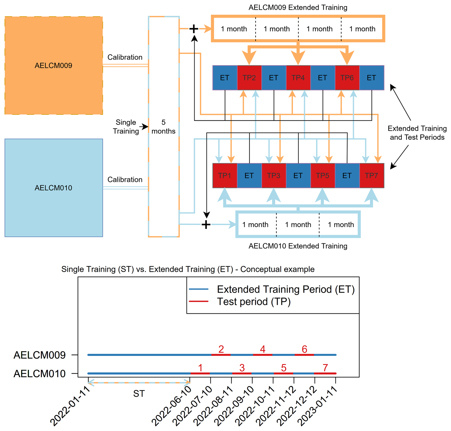
Figure 2 Schematic representation of the pairwise calibration strategy and calibration model development as a flow diagram (top) and a time series scheme (bottom) using two LCS measurement systems (AELCM009 and AELCM010). The ST period (11 January–10 June 2022) and the ET period as well as the numbered one-month test periods (TPs) for each LCS measurement system are shown. The thickness of the coloured lines in the flow diagram visually represents the amount of training data used for ET of the calibration model compared to ST.

The outline of the approach is shown in Fig. 2. Since the primary goal of an air quality monitoring system equipped with LCSs is to collect continuous measurements from a location outside a station site used for collocation calibration, we simulated the use of two calibrated LCS measurement systems alternately in the field. These two LCS measurement systems were represented through AELCM009 and AELCM010. Using both AELCM units, we received a continuous time series of in situ air pollution measurements. These in situ measurements are represented through the test periods (TPs) in Fig. 2. By merging the blocks of continuous data (TP1 to TP7), we created a continuous time series in the field. Individual calibration models for each AELCM unit were trained using a ST period or an ET period. ST used approximately 5 months of hourly reference data and LCS data to train a final calibration model for each individual LCS. ET offered more training data across different seasons, which reflects the aspect of regular LCS recalibration using reference monitors at a collocation site to guarantee long-term consistent data quality. The ST served as a reference to investigate whether there is an actual benefit in extending the training period.

Figure 2 shows ET lengths of 1 month and the testing data blocks. We experimented with a length of 1, 2 and 3 months to study the influence on the model performance. In a LCS network setting, an ET length of 3 months would mean, that an AELCM unit would take in situ measurements for 3 months before being replaced by another calibrated AELCM unit. Therefore, the former unit can be relocated to the collocation site for 3 months to extend its training data and to quality check its data before switching places again with the latter unit. Please note, that we were restricted by the overall collocation campaign length of 1 year. Selecting 5 months for the ST period, as shown in Fig. 2, resulted in seven months being available to fit the following data blocks, which were defined by the ET lengths. Two- and three-month ETs created a remainder of 1 training month at the end of the measurement campaign, which we used as well for the ET to not waste training data.

For the ET setup all training data blocks were employed for training a calibration model. Thus, we performed an a posteriori evaluation of the introduced pairwise calibration strategy including the introduced calibration models and ET lengths based on different performance metrics.

2.7 Performance metrics and target values

To quantify the impact of using an ET approach compared to a ST approach, we mostly applied commonly used and recommended performance metrics in LCS studies (Karagulian et al., 2019; Concas et al., 2021) and target values provided by EPA and CEN (Duvall et al., 2021a, b; CEN/TS 17660-1:2021, 2021; CEN/TS 17660-2:2024, 2024). These performance metrics are the RMSE, R², mean absolute error (MAE), relative expanded uncertainty (REU), spearman rank correlation (Rs) as well as the regression slope and intercept. Here, a simple linear regression between model-calibrated LCS data and AEMS reference data provide the slope and intercept (Duvall et al., 2021a, b). Most of the mentioned metrics are commonly used to describe LCS calibration model performance in regards of bias, noise, linearity and error (Karagulian et al., 2019; Duvall et al., 2021a, b; Yatkin et al., 2022; Diez et al., 2022).

We analysed the consequences of ET by using a cohesive view of performance metrics and target values, introduced through state-of-the-art test programs. A major challenge for potential end-users of LCSs is to interpret the calculated performance metrics and thus to infer if a LCS is a good fit for an intended application (Diez et al., 2022). Recognized organizations linked with governmental bodies like CEN and EPA started to develop frameworks in the form of test protocols, which can be used to check the suitability of LCSs for air quality monitoring applications. We used the performance metrics and associated categorizations given by state-of-the-art test programs as a reference to contextualize our study results. However, we emphasize that due to methodological differences, our testing framework for air sensors does not fully align with those of EPA and CEN.

So far, the EPA offers target values for O₃, NO₂, CO, SO₂, PM_2.5 and PM₁₀ air sensors through their testing protocols. According to EPA, the introduced performance metrics and their corresponding target values are the result of the current state of knowledge, based on, for example, literature reviews, findings from other organizations that conduct routine sensor evaluations and EPA's own expertise in sensor evaluation research (Duvall et al., 2021a, b). The current EPA test protocols include target values for the RMSE, R², regression slope, intercept, standard deviation and coefficient of variation. We used most of these target values in our benchmark experiment to assess how our pairwise calibration strategy influences the recognition of the presented LCSs as NSIM devices as defined by EPA. In this study, we did not include the standard deviation or coefficient of variation. Since we used only two LCSs per air pollutant, our experimental setup did not fulfil the requirements to calculate both performance metrics according to EPA's test protocols.

The REU is a performance metric, which is used for the assessment of the compliance of data quality objectives (DQOs) set in the European Air Quality Directive (AQD) 2008/50/EC (Directive 2008/50/EC, 2008; Yatkin et al., 2022). The REU is used in LCS studies (Spinelle et al., 2015; Castell et al., 2017; Cordero et al., 2018; Bigi et al., 2018; Liu et al., 2019; Bagkis et al., 2021; Ratingen et al., 2021; Bagkis et al., 2022), yet it is not a common sight to describe measurement uncertainty (Karagulian et al., 2019). While LCSs currently cannot meet the strict requirements for reference measurements in the AQD, their measurements can at least meet less strict DQOs. For this reason, LCSs can provide valuable supplemental information like indicative measurements next to regulatory fixed measurements provided by air quality stations for the assessment of air quality. This is acknowledged through the recently developed European TSs by CEN for gas sensors and PM sensors (CEN/TS 17660-1:2021, 2021; CEN/TS 17660-2:2024, 2024). Both CEN/TSs present classification schemes for LCSs, which respect the requirements for indicative measurements (class 1) and objective estimation (class 2) defined in the AQD Directive 2008/50/EC (2008). Furthermore, the CEN/TSs offer a classification for LCSs, being out of scope of the DQOs set in the AQD. Those LCSs fulfil more relaxed performance criteria and provide non-regulatory measurements (class 3). For instance, LCSs classified as class 3 air sensors can be applied in citizen science studies or can be used for educational purposes to raise environmental awareness. Finally, to classify the LCSs as class 1, class 2 or class 3 air sensor devices, we only used the REU estimated at the air pollutant limit values (LVs) in accordance with CEN/TSs (CEN/TS 17660-1:2021, 2021; CEN/TS 17660-2:2024, 2024). The LVs were obtained from CEN/TSs (CEN/TS 17660-1:2021, 2021; CEN/TS 17660-2:2024, 2024). The DQO of class 1, class 2 and class 3 correspond to specific REUs defined in the CEN/TSs for each air pollutant (Tables S1 and S2). Recently, the global air quality guidelines were updated by the World Health Organization (WHO) based on the latest systematic reviews of exposure-response studies (WHO, 2021). The European Union Parliament and the European Council agreed to a new revised AQD because of this development (Directive (EU) 2024/2881, 2024). The latest revised Directive (EU) 2024/2881 aligned its standards closer to the latest WHO air quality guidelines and introduced stricter LVs and updated DQOs for indicative measurements and objective estimation. Please note, that the presented CEN/TSs might change in the future to reflect the changes in Directive (EU) 2024/2881. It should also be noted that the LCS evaluation was performed only at a single urban background site (AEMS). The TSs by CEN call for evaluations at different sites, for instance, testing NO₂ sensors at traffic and background sites. To visualize the REU in the statistics software R we followed the study of Diez et al. (2022) as a reference, who made their code and data available. Furthermore, we used different smoothers (GAM, LOESS) in the REU figures depending on the sample size of the calibration data (Figs. 9, 10, 11, 12).

We calculated the REU according to the Guide for the Demonstration of Equivalence (GDE) following the introduced CEN/TSs (GDE, 2010; CEN/TS 17660-1:2021, 2021; CEN/TS 17660-2:2024, 2024). The REU is calculated through Eq. (1):

$$\begin{array}{}\text{(1)}& \begin{array}{rl}\mathrm{REU}\left(y_i\right)=& {\displaystyle \frac{\mathrm{2}{\left(\frac{\mathrm{RSS}}{\left(n-\mathrm{2}\right)}-u^{\mathrm{2}}\left(x_i\right)+{\left[b_{\mathrm{0}}+\left(b_{\mathrm{1}}-\mathrm{1}\right)x_i\right]}^{\mathrm{2}}\right)}^{\mathrm{1}/\mathrm{2}}}{y_i}}\\ & \times \mathrm{100},\end{array}\end{array}$$

with

$$\mathrm{RSS}=\sum {\left(y_i-b_{\mathrm{0}}-b_{\mathrm{1}}{x}_i\right)}^{\mathrm{2}},$$

where b₀ is the intercept and b₁ the slope of the orthogonal regression of y_i against x_i. x_i are the reference measurements given through the measurement instruments of the AEMS and y_i are the model-calibrated LCS measurements provided by the AELCM units, which together form n pairs of observation data. RSS is the residual sum of squares resulting from the orthogonal regression. u describes the uncertainty of the AEMS measurement instrument, which was obtained for every AEMS measurement instrument through the CEN/TSs (CEN/TS 17660-1:2021, 2021; CEN/TS 17660-2:2024, 2024).

Table 3 Statistics based on the hourly means of the different atmospheric variables measured by the AEMS from January 2022 to January 2023. For the calculation of the Rs all raw hourly LCS data for every individual sensor are used from AELCM009 and AELCM010. The AEMS data are used as reference for the correlation.

3 Results and discussion

3.1 Air pollution and meteorological situation

The environmental conditions and pollution concentrations based on hourly means are provided in Table 3. In our work, every LCS showed the premise of being a good-quality source of information according to the Rs (Table 3). We used the hourly means of the raw output of the LCSs and of the reference station AEMS to calculate Rs. In view of the observed gas concentration ranges in Table 3 and the LVs in the CEN/TS, it can be inferred that the LVs for CO (10 mg m⁻³) and NO₂ (200 µg m⁻³) were not reached at the measurement site. Thus, we could not classify the sensors according to CEN/TS 17660-1:2021 (2021). Classifications according to CEN/TS 17660-1:2021 (2021) and CEN/TS 17660-2:2024 (2024) were possible for O₃ and PM_2.5 since the hourly LV for O₃ (120 µg m⁻³) and the daily LV for PM_2.5 (30 µg m⁻³) were reached in their respective TPs. Given the observed concentration ranges for each air pollutant at our urban background collocation site (Table 3), we decided to do an in-depth analysis focussing on the O₃ and PM_2.5 LCSs in this study. Nevertheless, the analytical results for the employed CO and NO₂ LCSs are provided in the Supplement of this study. This is because the thresholds for the averaged concentrations of each air pollutant at the urban background collocation site were met at least once, as recommended by EPA (Duvall et al., 2021a, b). The recommended thresholds are 1 h average concentrations of 60 ppb for O₃, 30 ppb for NO₂, and 500 ppb for CO. The recommended threshold for the 24 h average is 25 µg m⁻³ for PM_2.5. The EPA suggests that these averaged concentrations must be reached at least once during a (30 d) TP (Duvall et al., 2021a, b).

3.2 Baseline single training results

We evaluated the calibration model output with respect to the training period and TP of each LCS targeting a specific air substance. The performance metrics in Table 4 highlight the general robustness and overall good performance of the found calibration models. All LCS models for O₃ and PM_2.5 for both AELCM boxes were able to reflect well the patterns in the reference data. For the O₃ calibration models, R² ranged from 0.92 to 1.00 during the training period and from 0.93 to 0.98 during the TP. For the PM_2.5 calibration models, R² ranged from 0.93 to 0.97 during the training period and from 0.84 to 0.93 during the TP. Considering the sensor error target by EPA (RMSE ≤ 5 ppb), it was reached for every O₃ sensor calibration model applied to the training period (RMSE: 0.80–4.35 ppb). It was mostly reached or at least approached during the TP (RMSE: 3.62–5.84 ppb). Instead of hourly means, the recommended performance metrics and target values by EPA for PM_2.5 are based on 24 h averages (e.g. RMSE ≤ 7 µg m⁻³). Nevertheless, given the results for the model-adjusted hourly means of the PM_2.5 air sensor output for the training period (RMSE: 1.45–2.51 µg m⁻³) and the TP (RMSE: 2.04–3.02 µg m⁻³), the PM_2.5 sensor error target was met for each calibration model if this criterion is applied to hourly means.

Table 4 Performances of LCS calibration models (MLR, RR, XGB, RF) for O₃ and PM_2.5 for each AELCM box using hourly means. Results are for the O₃ training dataset (11 January, 19:00:00–10 June 2022, 18:00:00 CET) and O₃ test dataset (10 June 2022, 19:00:00–11 January 2023, 17:00:00 CET) as well as for the PM_2.5 training dataset (11 January, 19:00:00–10 June 2022, 18:00:00 CET) and PM_2.5 test dataset (10 June 2022, 19:00:00–7 January 2023, 00:00:00 CET).

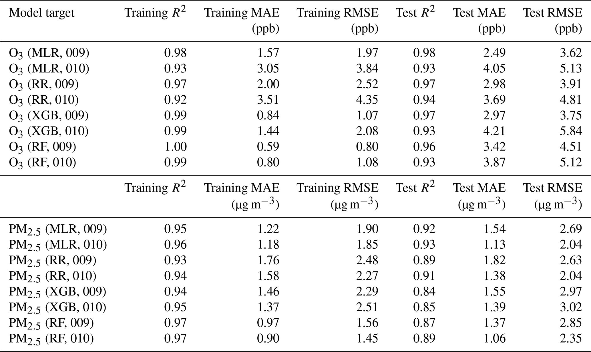
While the O₃ sensor calibration models based on the machine learning techniques RF and XGB performed the best in regards of R², MAE and RMSE in the training period, it is not the case in the TP. Table 4 shows the results of a single calibration using different calibration models, which are trained on data from January to June 2022 (ST period). The tree-based algorithms represented through RF and XGB have the constraint, that they are bound by their calibration space (Bigi et al., 2018). Tree-based models can only estimate within the bounds of the calibration space (Bigi et al., 2018), which is defined by the training dataset, and show poor extrapolation ability (Yu et al., 2024). MLR and RR do not have a constraint like tree-based models in regards of calibration space. Given the described limitations of tree-based models, it is understandable that their performance decreases more strongly from the training to the test period compared with the MLR and RR approaches. MLR and RR calibration models seem to be an appropriate choice for low-cost O₃ air sensors in a ST setup. Apparently, there is no meaningful performance benefit in using tree-based calibration models given the calculated performance metrics for the TP in Table 4. The same holds true for PM_2.5. Given that a training period spans several months, MLR and RR calibration models should be used instead of tree-based models, if the goal is to calibrate the chosen O₃ and PM_2.5 LCSs in a ST setup. This is further explained in Sect. 3.3.

Identical LCS units like the calibrated AS-B431 and SAG-SPS30 units performed differently at the same location when inspecting the calculated R², RMSE and MAE values. The raw output data produced by the AS-B431 for O₃ (net voltages) and the SAG-SPS30 for PM_2.5 (mass concentrations) of both AELCM boxes were almost perfectly correlated (R² ≥ 0.97) during the collocation period. This implies changes in sensor signals were responses to changing environmental conditions (e.g. air pollution, ambient temperature and humidity) and not related to sensor-to-sensor variability. Bittner et al. (2022) reported the same behaviour for Alphasense EC gas sensors. Performance differences between the same LCS model units after calibration are possibly related to the varying performance of the other sensors used in the LCS calibration models.

3.3 Extended training results and EPA performance targets

To assess seasonal differences in air sensor performance we calculated the suggested performance metrics by EPA on a 30 d basis, namely the RMSE (error), R² (linearity), slope (bias) and intercept (bias). The EPA also provided target values for each of these performance metrics, which are highlighted in red in the circular bar plots (e.g. Fig. 3). We used the absolute value of the calculated intercept and the difference between the calculated model slope and the ideal slope of 1. We did this for each calibration model to improve the interpretability of the figures. The original intercepts and slopes can be found in the Supplement (Tables S29–S52). Circular bar plots are a visual tool to evaluate the benefit of using the ET instead of the ST approach to enhance the qualitative and quantitative validity of calibrated LCS output. In addition, they enhance the visual distinction between the different calibration techniques, i.e. MLR, RR, and the machine learning algorithms RF and XGB.

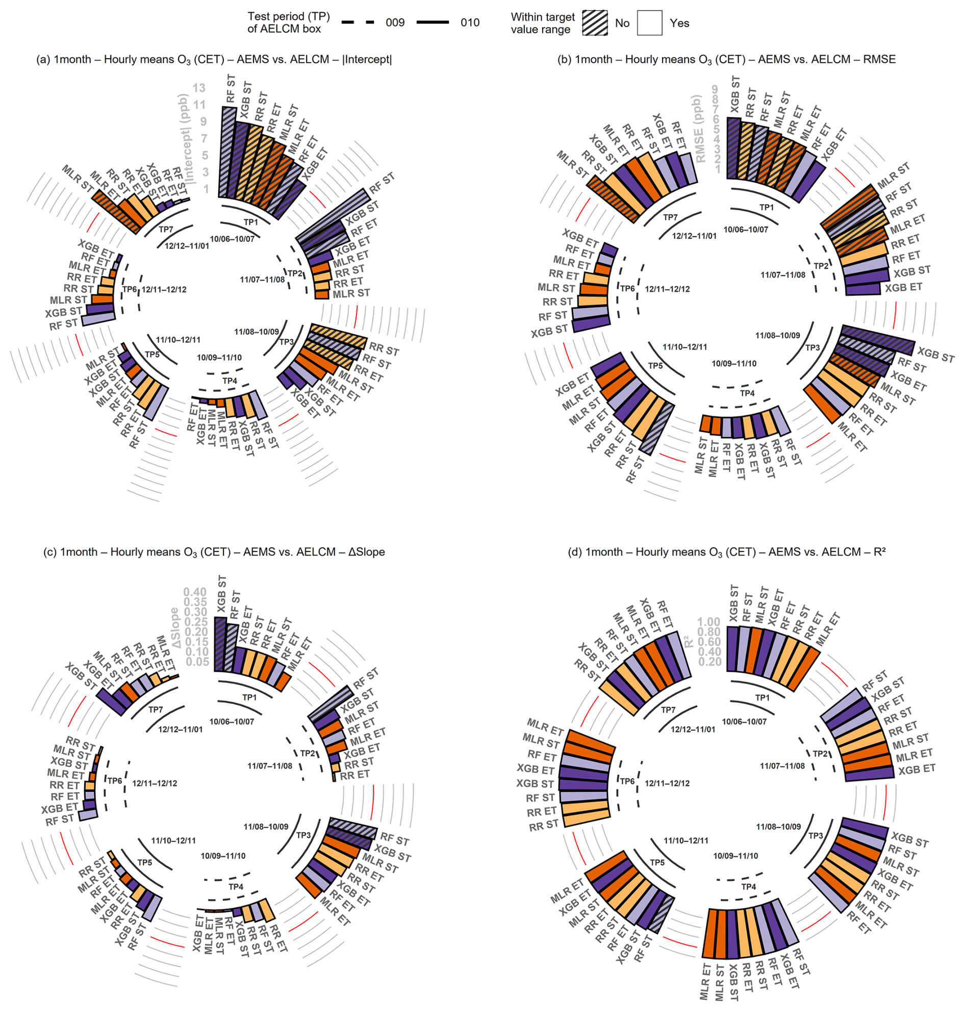
Figure 3 Performance metrics of the single O₃ LCS in each AELCM box, calculated from hourly mean values after calibration. Metrics are presented for each calibration model, TP, and calibration variant (ST and ET). Models are ordered by performance from highest to lowest in each period. The ET is characterized by the one-month variant for each AELCM box. Values highlighted in red describe the least accepted target value given by EPA for each performance metric (|Intercept| (a), RMSE (b), ΔSlope (c), R² (d)).

For the most part, O₃ sensor calibration model performance benefitted from an ET. According to Figs. 3, 4 and 5, the performance gains highly varied in magnitude depending on the performance metric (Intercept, slope, RMSE, R²), ET length (1 month to 3 months) and calibration model (MLR, RR, RF and XGB). For ETs of 1 month, 2 months and 3 months and for each calibration model both calibrated O₃ sensors correlated quite well with the hourly reference data during summer, autumn and winter. This is reflected through R² (R² (ST): 0.79–0.98; R² (ET): 0.86–0.98). Only once the target value range for R² was missed, which was for AELCM010 and the RF calibration model in TP5 for the ST variant. But an ET resulted in reaching the target value range for R² in TP5 for this calibration model. To summarize, a ST period of 5 months was almost sufficient to reach the target value range for R² (R² ≥ 0.80) for each TP and O₃ sensor calibration model. High R² values for the calibrated O₃ sensor units of the same type (AS-B431) for periods associated with Northern Hemisphere winter and warmer months (“ozone season”) are in agreement with other LCS studies (Zimmerman et al., 2018; Zauli-Sajani et al., 2021). For all ET configurations, the performance of MLR and RR in terms of R² was comparable to the RF and XGB machine learning techniques.

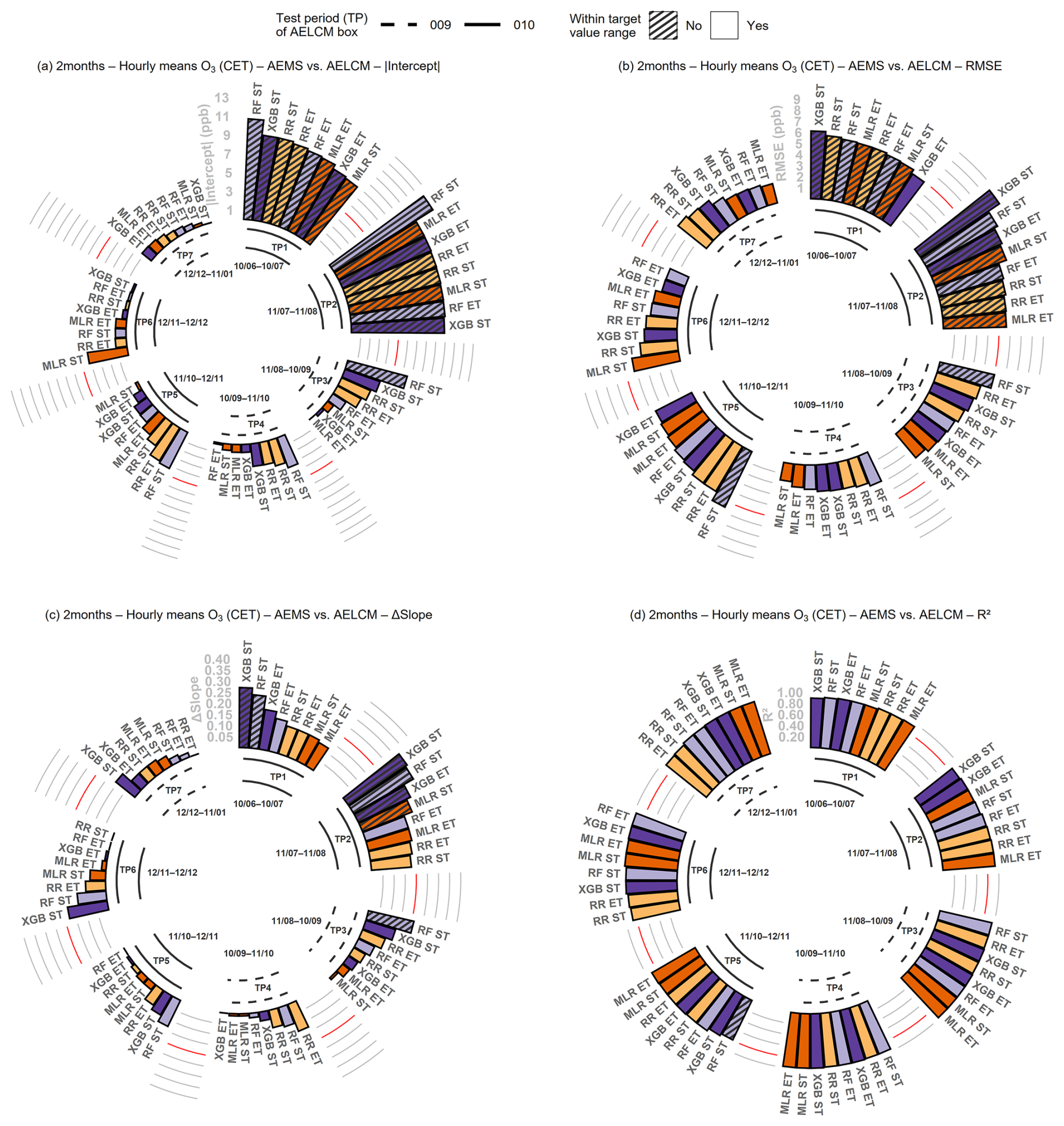
Figure 4 Performance metrics of the single O₃ LCS in each AELCM box, calculated from hourly mean values after calibration. Metrics are presented for each calibration model, TP, and calibration variant (ST and ET). Models are ordered by performance from highest to lowest in each period. The ET is characterized by the two-month variant for each AELCM box. Values highlighted in red describe the least accepted target value given by EPA for each performance metric (|Intercept| (a), RMSE (b), ΔSlope (c), R² (d)).

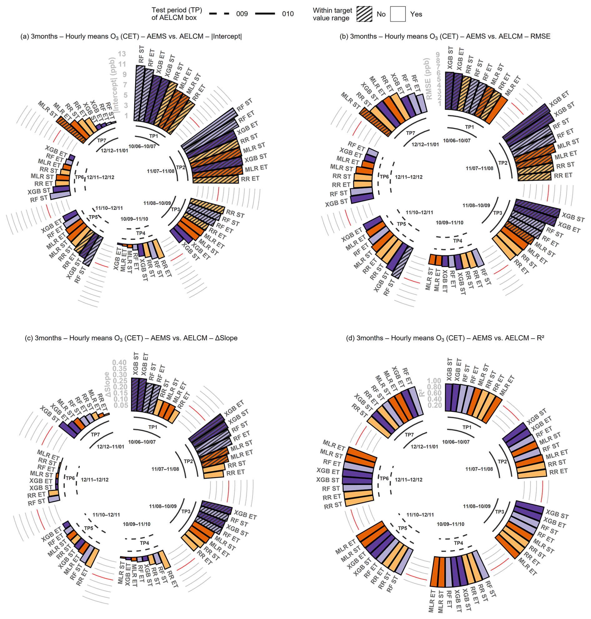
Figure 5 Performance metrics of the single O₃ LCS in each AELCM box, calculated from hourly mean values after calibration. Metrics are presented for each calibration model, TP, and calibration variant (ST and ET). Models are ordered by performance from highest to lowest in each period. The ET is characterized by the three-month variant for each AELCM box. Values highlighted in red describe the least accepted target value given by EPA for each performance metric (|Intercept| (a), RMSE (b), ΔSlope (c), R² (d)).

We found a distinct difference in gas sensor performance for R² between warmer periods and colder periods for the employed NO₂ and CO sensors, which implied the existence of limiting factors in sensor calibration. Generally, TP4 (≈ September) was the first TP, where NO₂ and CO sensor calibration models entered the R² target range recommended by EPA for NO₂ sensors (R² ≥ 0.70) and CO sensors (R² ≥ 0.80) (Figs. S5, S6, S7, S12, S13, S14). In the following months (TPs), NO₂ and CO sensor calibration models were available, which performed in the boundaries of their targeted R² range. We assume for TP1 till TP3, that an interplay between environmental interferences and limited sensor sensitivity at lower ambient concentrations of NO₂ and CO played a crucial role for the overall low sensor performances in those warmer periods. The findings in other studies support this assumption (Cross et al., 2017; Hagan et al., 2018). The mean reference values for NO₂, CO, air temperature and relative humidity for each TP can be found in the Supplement (Figs. S3 and S4). In the warmer periods, MLR and RR LCS calibration models performed notably worse for NO₂ sensors, as reflected in the R² values. The increased air temperatures at low pollutant concentrations during these periods might have introduced non-linearities to the sensor signals (Cross et al., 2017; Hagan et al., 2018). Consequently, non-linear models (RF and XGB) outperformed linear models (MLR and RR).

An extension of the training period for the O₃ and PM_2.5 calibration models had overall only a small impact on R², when comparing the LCS calibration models between their ST and ET variants (Figs. 3, 4, 5, 6, 7, 8). R² values only occasionally experienced stronger positive changes between at least 0.05 and 0.09 through ET for some TPs and mainly for the O₃ LCSs and the RF and XGB calibration models (Tables S29–S52). The correlative performance of the O₃ and PM_2.5 calibration models for ST were already quite high. The calibrated PM_2.5 sensors correlated quite well with the daily reference data during summer, autumn and winter (R² (ST): 0.76–0.99; R² (ET): 0.79–0.99). This was observed for ETs of 1 month, 2 months and 3 months and for each calibration model. A ST period of 5 months was sufficient to reach the target value range for R² (R² ≥ 0.70) for each TP and PM_2.5 sensor calibration model. High R² values for the calibrated PM_2.5 sensor units (SAG-SPS30) for periods associated with Northern Hemisphere winter (heating season) and warmer months are in agreement with other LCS studies. In these studies the same sensor type was factory-calibrated or model-calibrated (Vogt et al., 2021; Gäbel et al., 2022; Shittu et al., 2025). Distinctive benefits for applying an ET to calibration models were rather identified for performance metrics, which describe the bias and error.

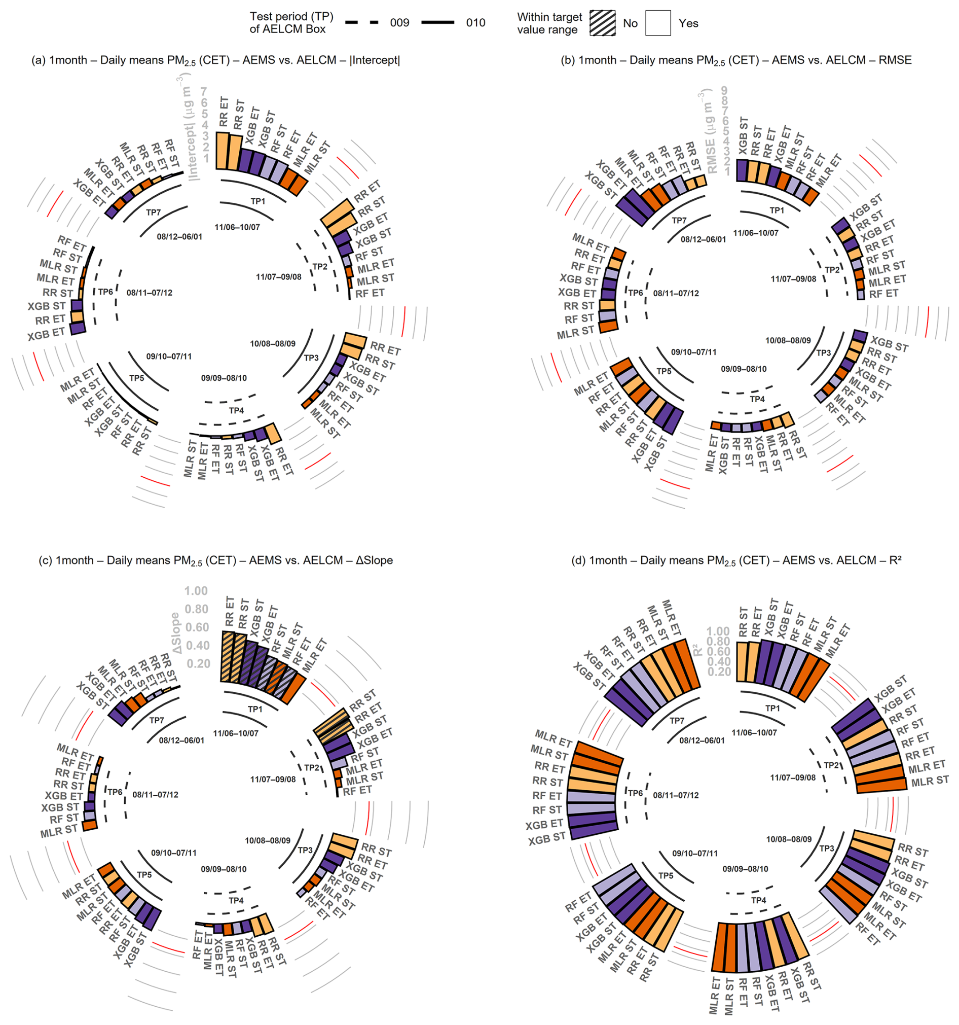
Figure 6 Performance metrics of the single PM_2.5 LCS in each AELCM box, calculated from daily mean values after calibration. Metrics are presented for each calibration model, TP, and calibration variant (ST and ET). Models are ordered by performance from highest to lowest in each period. The ET is characterized by the one-month variant for each AELCM box. Values highlighted in red describe the least accepted target value given by EPA for each performance metric (|Intercept| (a), RMSE (b), ΔSlope (c), R² (d)).

Figure 7 Performance metrics of the single PM_2.5 LCS in each AELCM box, calculated from daily mean values after calibration. Metrics are presented for each calibration model, TP, and calibration variant (ST and ET). Models are ordered by performance from highest to lowest in each period. The ET is characterized by the two-month variant for each AELCM box. Values highlighted in red describe the least accepted target value given by EPA for each performance metric (|Intercept| (a), RMSE (b), ΔSlope (c), R² (d)).

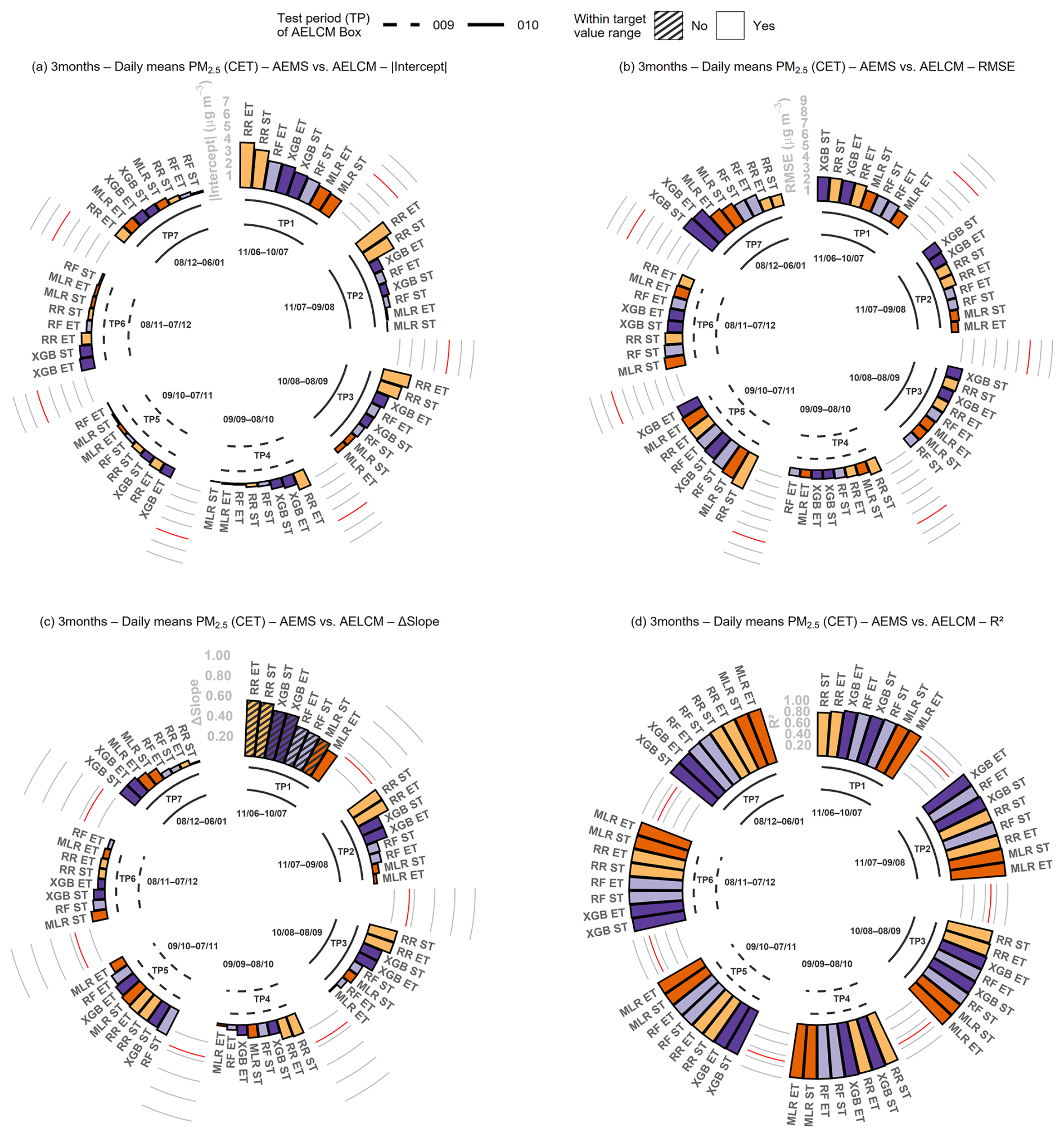
Figure 8 Performance metrics of the single PM_2.5 LCS in each AELCM box, calculated from daily mean values after calibration. Metrics are presented for each calibration model, TP, and calibration variant (ST and ET). Models are ordered by performance from highest to lowest in each period. The ET is characterized by the three-month variant for each AELCM box. Values highlighted in red describe the least accepted target value given by EPA for each performance metric (|Intercept| (a), RMSE (b), ΔSlope (c), R² (d)).

Using ST, our LCS calibration models were trained on data between January and June. The TPs TP1 till TP3 (≈ June–September) in Figs. 3, 4 and 5 are the most relevant TPs for the assessment of the performance (Intercept, slope, RMSE) of our O₃ sensor calibration models. This is due to elevated O₃ concentrations and the health relevance of O₃ during these periods in the Northern Hemisphere (Hertig et al., 2019; Jahn and Hertig, 2021). TP1 is the only period, where we can see a change in performance of LCS calibration models for a single O₃ sensor (AELCM010) depending on ET length over all introduced ET lengths (ETs of 1, 2 and 3 months).

Overall, the bias worsens with ET lengths of 2 months and 3 months. The most pronounced degradation of intercept and slope can be seen for RF and XGB. A reduction of the amount of summer training data provided by AELCM010 leads to a meaningful reduction of the calibration space for the XGB and RF calibration models. While the XGB calibration model with ETs of 1 month almost reached the intercept target value range (|Intercept| ≤ 5 ppb) in TP1, not a single calibration model even approached the target value range with other ET lengths. The RF and XGB calibration models using only ST and ETs of 3 months were outside the slope target value range (ΔSlope ≤ 0.2) in TP1. The decrease in performance was also reflected in a decrease of the number of calibration models, which were within the target value range for the RMSE (RMSE ≤ 5 ppb). Most calibration models did not achieve the target RMSE range during TP1. At most two models achieved a sufficiently low RMSE in TP1, both using ET lengths of 1 month (XGB and RF). Considering all calculated performance metrics derived from Figs. 3, 4 and 5 in TP1, the XGB calibration model with ETs of 1 month was almost able to reach all target values provided by EPA. Looking at TP1 and TP3 with respect to bias and error, in general XGB and RF calibration models suffered the most under a lack of training data (ST variant) and a loss of summer training data due to longer ETs. The former scenario reflects an absence of recalibration, whereas the latter reflects a reduced recalibration cycle (two- and three-month variants). Comparing the MLR and RR calibration models with XGB and RF calibration models for AELCM010 in terms of bias and error in TP1, TP2 and TP3, it becomes evident that applying ET to the machine learning techniques can yield substantial improvements. In contrast, the absence of ET may result in markedly higher bias and error. In these periods the impact on bias reduction and error reduction due to an ET is more pronounced for the RF and XGB calibration models related to the O₃ sensor employed with AELCM010.

Considering our experimental setup at an urban background site as well as the calculated bias and error metrics for TP1 to TP7, we conclude the following for LCS air pollution studies that aim to make quantitative statements about O₃ employing AS-B431 sensor units: (1) MLR and RR calibration models should be employed when ET cannot be applied, but a single multi-month training period is available, which accounts for seasonal variations in atmospheric conditions (meteorological and air pollution factors) and thus a wide range of environmental influences on the sensor signal. (2) If ET is applicable in the form of monthly recalibration, RF and XGB calibration models appear to be the most sensible choice.

Unlike for O₃, all TPs shown in Figs. 6, 7 and 8 were relevant for assessing the performance of our PM_2.5 sensor calibration models. From a health perspective, unhealthy levels of PM_2.5 can be present throughout the year due to the diverse sources of ambient PM_2.5. Main anthropogenic sources include industrial emissions, ground transport emissions, biomass burning and the secondary formation of fine PM classified as PM_2.5 (Thunis et al., 2021; Gu et al., 2023; Chowdhury et al., 2023; Zauli-Sajani et al., 2024). Natural sources of fine particles include wildfires (Chowdhury et al., 2024) and dust events, such as Saharan dust transported to different latitudes (Varga et al., 2021). Generally, weather conditions and the atmospheric state influence the transport, mixing ratio, transformation and deposition of air substances; hence they are important factors defining the air quality level (Russo et al., 2014, 2016; Bodor et al., 2020; García-Herrera et al., 2022; Dayan et al., 2023; Du et al., 2024).

A MLR calibration model was the only one that satisfied all EPA recommendations for PM_2.5 sensor bias (|Intercept| ≤ 5 µg m⁻³; ΔSlope ≤ 0.35) in all TPs, which is shown in Figs. 6, 7 and 8. Here, the MLR calibration model with ET reached the target range for the slope in TP1, which the other calibration models did not. The intercept target range was met by all calibration models with ST in each TP. No ET was needed here. The same applied for the PM_2.5 sensor error target range (RMSE ≤ 7 µg m⁻³). Considering how often a MLR calibration model was the best performing model in regards of sensor bias and sensor error, we conclude that a MLR calibration model is sufficient to improve the quantitative validity of raw SAG-SPS30 data. RF and XGB did not offer a substantial alternative, visible by their performance metrics. This is emphasized for instance in Fig. 7, where the best-performing machine learning model, RF with ET, barely offers more than a small performance improvement compared to a MLR calibration model with ST. Looking at all ST and ET calibration models, there is generally very little change in quantitative performance following an ET approach. In our collocation experiment, the chosen ST period appears to be sufficient to train robust calibration models, which perform well in the following TPs in an urban background setting. Therefore, recalibration appears largely unnecessary for the SAG-SPS30 when considering only the EPA performance targets discussed in this section, rather than the more stringent DQOs outlined in Sect. 3.4. This is particularly notable given that both the RF and MLR calibration models, trained using the ST period, nearly met the slope target range in TP1.

A calibrated SAG-SPS30 performed usually well in all performance categories in each TP. This could be due to the raw sensor data quality, which may be influenced by the technical integration of the measurement principle into the SAG-SPS30, or the out-of-the-box calibration algorithm provided by Sensirion (Vogt et al., 2021). Our calibration models may have benefited from both aspects. Meeting the EPA performance recommendations through LCS calibration was less challenging for a SAG-SPS30 than for the Alphasense EC gas sensors. An ET is recommended to achieve the best possible sensor performance for Alphasense EC gas sensors. They are likely more challenging to maintain because gas sensor performance is strongly influenced by local atmospheric conditions that vary seasonally. In addition, Alphasense EC gas sensors experience a more pronounced sensor ageing compared to SAG-SPS30 units. Therefore, more frequent pairwise recalibrations are expected to improve the calibration process. Our performance results implied (Figs. 3–5, S5–S7, S12–S14, Tables S5–S40), that the EC LCSs AS-B431, AS-B43F and AS-B4 benefit the most from a pairwise recalibration every 30 d (one-month ET variant), where the pairwise calibration gets extended by another 30 d. With two AELCM units and monthly recalibrations, both units can be recalibrated within the same season while uninterrupted in situ data collection continues. This allows us to account for sensor ageing and changing environmental conditions. Our results, together with those of other studies, show that the likelihood of well performing calibration models for the employed LCSs increases with a sufficient amount of training data (Zauli-Sajani et al., 2021; Nowack et al., 2021). Moreover, LCS calibration benefits from raw LCS measurement data that are not dominated by noise at low concentrations because of sensor sensitivity limits (Zimmerman et al., 2018).

3.4 Extended training results and data quality objectives

The EU AQDs Directive 2008/50/EC (2008) and the new Directive (EU) 2024/2881 (2024) provide DQOs for regulatory-grade measurement devices, which LCSs are not. But LCSs have a legitimate role alongside those regulatory-grade monitoring systems as air sensors for indicative measurements and objective estimation. We applied REU plots to analyse the possible end-use applications of the employed calibrated AELCM sensors, considering the DQOs and LVs for air sensor classification provided by the CEN/TSs. The DQOs used in the sensor test protocols CEN/TS 17660-1:2021 (2021) and CEN/TS 17660-2:2024 (2024) are based on Directive 2008/50/EC (2008). REU plots helped to describe the measurement uncertainty “point by point” of the calibrated LCSs, complementing the use of single-value error metrics (global performance metrics) applied in Sect. 3.2 and 3.3 (Diez et al., 2024). They provide deeper insight into the error structures and information content of calibrated LCS data (Diez et al., 2022).

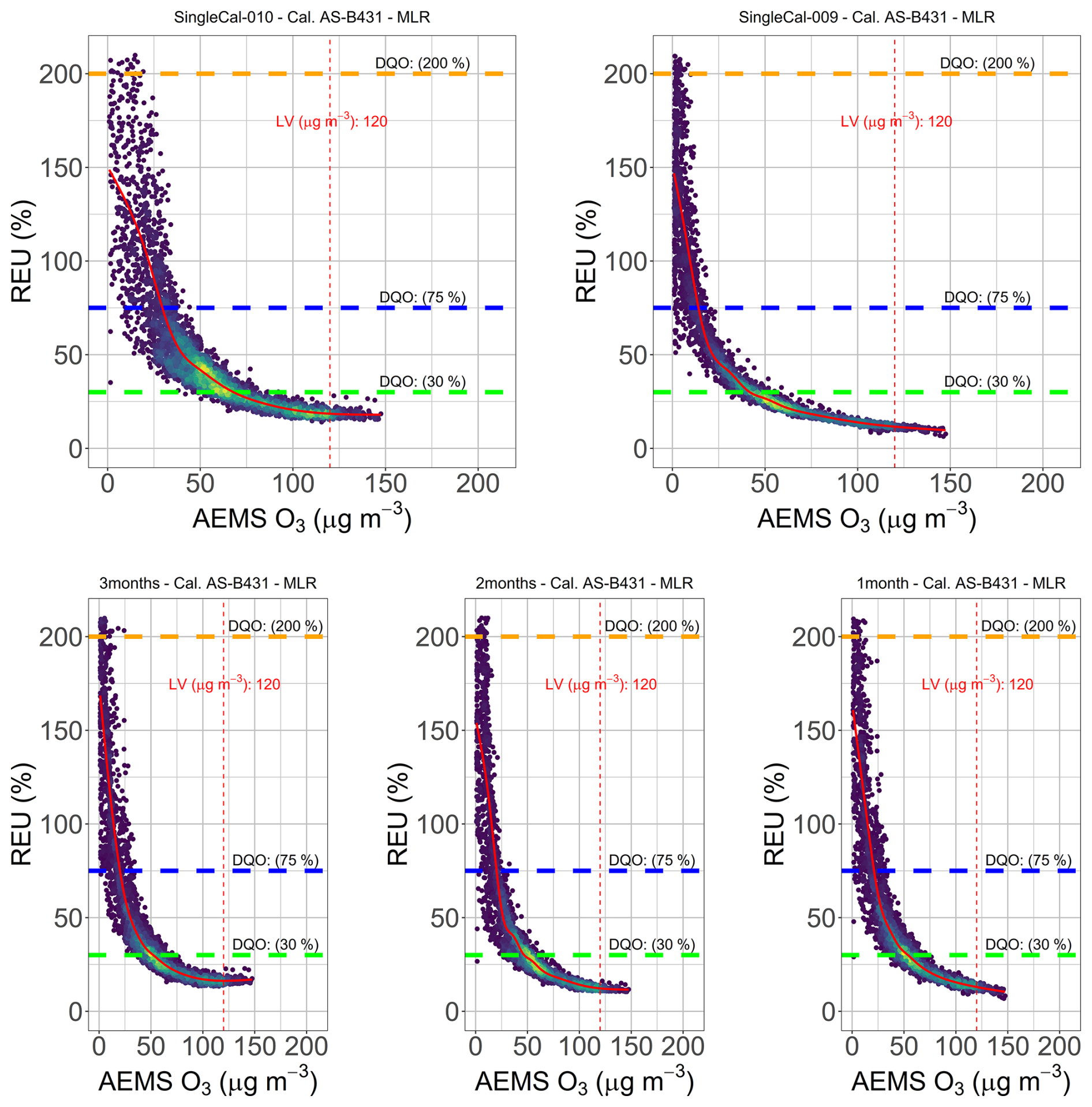
Figure 9 Calculated REU values for MLR calibrated O₃ LCS hourly data belonging to the TPs (TP1–TP7, 10 June 2022–11 January 2023) of AELCM009 and AELCM010. The calibration variants are ST (top row, left: AELCM010, right: AELCM009) and ET (bottom row). The ET is characterized by ET variants of 1, 2 and 3 months for each AELCM box. Horizontal dashed lines describe the DQOs (O₃ Class 1 DQO = 30 %, Class 2 DQO = 75 % and Class 3 DQO = 200 %). The vertical dashed line describes the limit value for O₃ (LV = 120 µg m⁻³). The fitted smooth curve (red) is based on a generalized additive model (GAM). Data density is shown through colour, where darker colours express lower data density and brighter colours express higher data density.

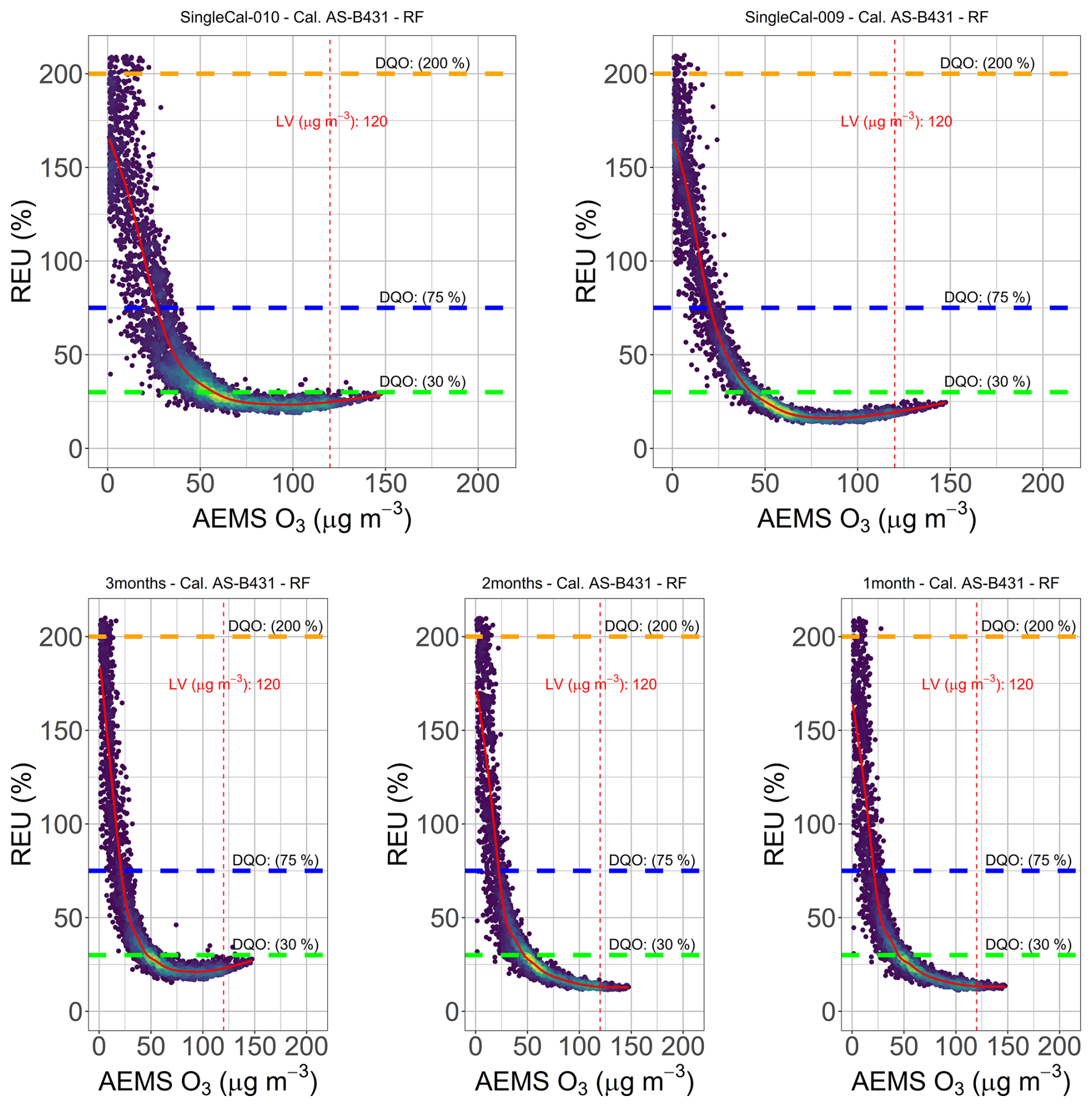
Figure 10 Calculated REU values for RF calibrated O₃ LCS hourly data belonging to the TPs (TP1–TP7, 10 June 2022–11 January 2023) of AELCM009 and AELCM010. The calibration variants are ST (top row, left: AELCM010, right: AELCM009) and ET (bottom row). The ET is characterized by ET variants of 1, 2 and 3 months for each AELCM box. Horizontal dashed lines describe the DQOs (O₃ Class 1 DQO = 30 %, Class 2 DQO = 75 % and Class 3 DQO = 200 %). The vertical dashed line describes the limit value for O₃ (LV = 120 µg m⁻³). The fitted smooth curve (red) is based on a generalized additive model (GAM). Data density is shown through colour, where darker colours express lower data density and brighter colours express higher data density.

Figures 9 and 10 show the “point by point” LCS measurement uncertainty for the “classical” MLR O₃ calibration models and the machine learning-based RF O₃ calibration models. The fluctuation in measurement uncertainty across the observed range was greater for the calibrated O₃ LCS data of AELCM010, which is shown in the top rows of the REU plots. The ST calibrated O₃ LCS data of AELCM009 and AELCM010 met the class 1 DQO (REU ≤ 30 %), but the calibrated data of AELCM009 reached it more reliably even at lower measured concentrations. The REU values at the O₃ LV of 120 µg m⁻³ indicate that both calibrated O₃ LCSs can be classified as class 1 sensor systems. Therefore, both air sensors can be used for indicative measurements. It must be said that we did not follow all activities and principles, which are relevant for the classification according to CEN/TS 17660-1:2021 (2021) and CEN/TS 17660-2:2024 (2024). This includes laboratory tests, which were not part of this study.

As in Sect. 3.2, differences in performance between identical LCS units are evident once more. In this case, they are visually detectable across the entire observed concentration range of ambient O₃. Global performance metrics (e.g. RMSE, R², MAE) cannot reflect this aspect (Diez et al., 2022). The top rows in both figures (also Figs. S19 and S20) depict a differing response of the employed calibrated sensor units to the same environmental conditions experienced at the station site during the collocation period. Possible reasons for these differences in sensor behaviour were explained in Sect. 3.2. Extending the calibration model training period and therefore expanding the calibration space is advised for machine learning methods, as evidenced by the REU plots in Figs. 10 and S19. In the three-month ET variant, AELCM010 was active in TP1 to TP3, the time when the highest O₃ concentrations were observed (Fig. S1). In the two-month and one-month ET variants, AELCM009 was active in TP3 and TP2, in that order. The lack of further summer training data in the three-month ET variant resulted visibly in increased REU values above 100 µg m⁻³ (Fig. 10, bottom left) for AELCM010. The other two ET variants provide further summer training data to each RF calibration model used for the O₃ LCSs belonging to AELCM009 and AELCM010. This resulted in a reduced measurement uncertainty for higher concentrations in TP1 until TP3 (Fig. 10, bottom middle and bottom right), being not the case for both RF calibrated LCSs using only ST (Fig. 10, top row). If pairwise calibration is considered for a LCS measurement campaign, we recommend using two calibrated LCSs meeting the same DQO, in order to ensure consistent in situ data quality as demonstrated in Figs. 9 and 10.

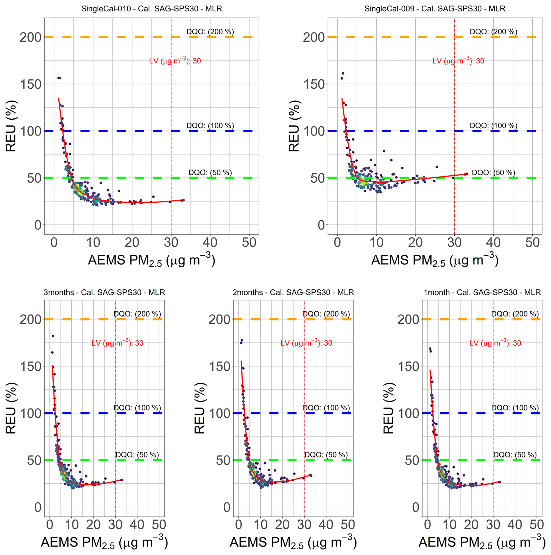
Figure 11 Calculated REU values for MLR calibrated PM_2.5 LCS daily data belonging to the TPs (TP1–TP7, 11 June 2022–6 January 2023) of AELCM009 and AELCM010. The calibration variants are ST (top row, left: AELCM010, right: AELCM009) and ET (bottom row). The ET is characterized by ET variants of 1, 2 and 3 months for each AELCM box. Horizontal dashed lines describe the DQOs (PM_2.5 Class 1 DQO = 50 %, Class 2 DQO = 100 % and Class 3 DQO = 200 %). The vertical dashed line describes the limit value for PM_2.5 (LV = 30 µg m⁻³). The fitted smooth curve (red) is based on locally estimated scatterplot smoothing (LOESS). Data density is shown through colour, where darker colours express lower data density and brighter colours express higher data density.

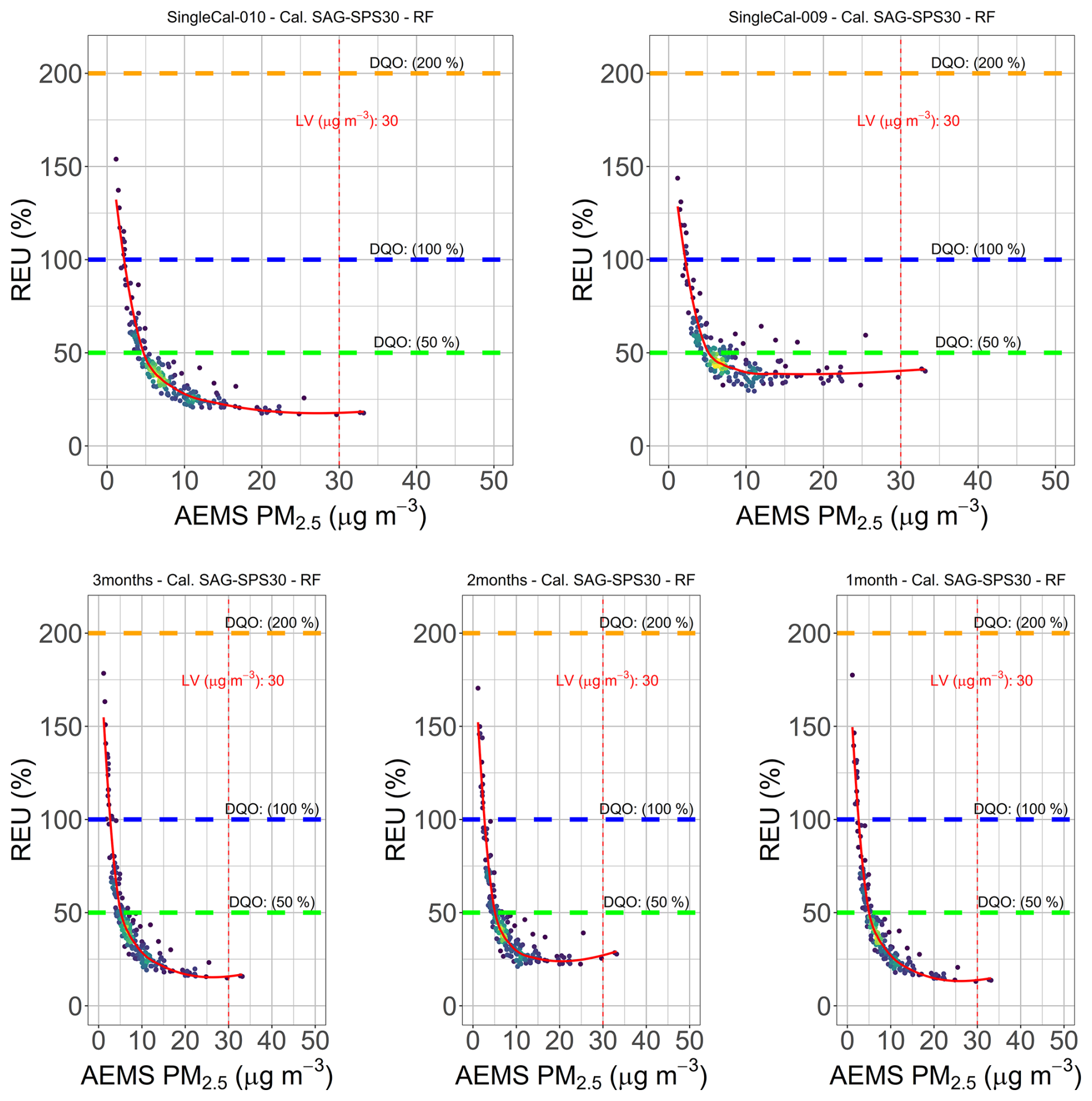
Figure 12 Calculated REU values for RF calibrated PM_2.5 LCS daily data belonging to the TPs (TP1–TP7, 11 June 2022–6 January 2023) of AELCM009 and AELCM010. The calibration variants are ST (top row, left: AELCM010, right: AELCM009) and ET (bottom row). The ET is characterized by ET variants of 1, 2 and 3 months for each AELCM box. Horizontal dashed lines describe the DQOs (PM_2.5 Class 1 DQO = 50 %, Class 2 DQO = 100 % and Class 3 DQO = 200 %). The vertical dashed line describes the limit value for PM_2.5 (LV = 30 µg m⁻³). The fitted smooth curve (red) is based on locally estimated scatterplot smoothing (LOESS). Data density is shown through colour, where darker colours express lower data density and brighter colours express higher data density.

Figures 11 and 12 show the “point by point” LCS measurement uncertainty for the PM_2.5 calibration models based on MLR and RF. The MLR and RF calibrated PM_2.5 datasets of AELCM009 exhibited greater measurement uncertainty across the observed daily means of PM_2.5. This is evident when comparing the ST calibrated datasets of AELCM009 and AELCM010 (Figs. 11 and 12, top row): REU values related to AELCM009 met the class 1 DQO (REU ≤ 50 %) less consistently compared to the REU values related to AELCM010. For the ST variant, the LOESS fits at the PM_2.5 LV of 30 µg m⁻³ indicate that the MLR calibrated PM_2.5 LCS of AELCM009 can be classified as a class 2 sensor system for objective estimation (REU ≤ 100 %), whereas the MLR calibrated PM_2.5 LCS of AELCM010 can be classified as a class 1 sensor system for indicative measurements. RF calibration models suggest that both PM_2.5 LCSs accomplish the highest tier of sensor systems (class 1), achieving indicative measurements at the PM_2.5 LV. Above 5 µg m⁻³ both RF calibrated PM_2.5 LCSs show (almost) consistently data meeting the class 1 DQO for the ST variant. The non-aligning patterns in relative error between the ST calibrated SAG-SPS30 units indicate that the employed calibrated sensor units respond differently under identical environmental conditions (Figs. 11, 12, S21, S22), as previously observed with the AS-B431 units measuring O₃.

ET for the MLR and RF calibration models helped to build continuous LCS time series data that met the class 1 DQO more consistently, using both calibrated SAG-SPS30 units (Figs. 11, 12, bottom row). ET to achieve more consistency in data quality was especially relevant for the PM_2.5 LCS employed with AELCM009. Figure 12 shows, that an ET characterized by the one-month variant was the most beneficial to reduce measurement uncertainty for higher concentrations of PM_2.5. We conclude that higher sensor system tiers for LCSs can be achieved through ET, thereby broadening the scope of applications for a LCS.

3.5 Implications for sustainable LCS networks and future outlook

Our concept for an effective, sustainable and manageable LCS network focuses on identifying the main target population for health protection from environmental exposures, such as air pollution and heat. This focus takes into account the advantages and disadvantages of current LCS technology. We consider the most vulnerable people as our main target group, for instance children, elderly people, outdoor workers or people with pre-existing health conditions. LCS measurements can thus be placed at locations with a high density of vulnerable populations, such as retirement homes, schools, kindergartens, or outdoor workplaces. Therefore, we recommend focusing on the characteristics of the measurement scope rather than simply building a spatially dense LCS observation network. Reducing the amount of LCSs and efficiently placing them by figuring out at-risk population hotspots could reduce the management effort using a pairwise calibration strategy similar to the one we introduced in this study. Another benefit of following our calibration strategy could be improved error minimization of LCS data, particularly given that LCS devices are placed directly next to a reference station for (re-)calibration. This could result in higher LCS data quality compared to the use of complex in situ calibration strategies for error reduction and data quality control. Following our concept, continuous in situ data collection can be achieved by using a pair of regularly maintained LCSs at the same location.

Analysing whether LCS data fit their intended purpose and provide viable information for the end-use application over time remains a challenge, especially in the context of a long-term measurement campaign. Stricter DQOs for regulatory-grade air measurement instruments, as a result of the recently updated WHO global air quality guidelines (WHO, 2021), could indirectly limit the scope of end-use applications for LCSs. For example, CEN/TS 17660-1:2021 (2021) and CEN/TS 17660-2:2024 (2024) rely on Directive 2008/50/EC (2008). Both CEN/TSs help to define the possible end-use applications of sensor systems. Considering the relationship between the introduced CEN/TSs and the Directive 2008/50/EC, an update of both CEN/TSs due to the recently published Directive (EU) 2024/2881 (2024) is not unlikely. Sensor manufacturers are called upon to consult state-of-the-art scientific literature of the air sensor research community to accelerate technological advancement while the air sensor community is called upon to rethink how LCS networks are built and managed. The latter is important to ensure that LCS networks move beyond the status of test applications and gain recognition as long-term supplemental monitoring systems (Carotenuto et al., 2023). Such recognition facilitates their integration into official networks, allowing LCSs to benefit the most vulnerable members of society.

4 Conclusions

In an attempt to consistently provide air sensor performance by a pair of O₃ and PM_2.5 LCSs (AS-B431 and SAG-SPS30) suitable for supplementing official air quality monitoring networks, a still uncommon approach for recurrent sensor calibration was explored. This approach was tested during a yearlong collocation campaign at an urban background station next to the University Hospital Augsburg, Germany.

LCSs were collocated with regulatory-grade air measurement instruments and were exposed to a wide range of environmental conditions, with air temperatures between −10 and 36 °C, relative air humidity between 19 % and 96 % and air pressure between 937 and 983 hPa. The ambient concentration ranges were up to 82 ppb for O₃ and 153 µg m⁻³ for PM_2.5. LCS calibration models were built using linear regression techniques (MLR and RR) and machine learning (RF and XGB).

We used a pairwise (re-)calibration strategy to enable continuous in situ measurements with two alternating O₃ (PM_2.5) LCSs. The results were evaluated using novel air sensor performance targets defined by EPA test protocols and CEN/TSs. We recommend regular in-season ET, instead of relying on a single multi-month training period. These updates to the calibration models are necessary to consistently produce data with sufficient information content (indicative and NSIM-level measurements) from AS-B431 (SAG-SPS30) units to support existing official air quality monitoring. Our findings underscore the importance of rigorous LCS quality assurance and control for studies or LCS monitoring networks that aim to make quantitative assertions with LCSs.

Based on the EPA performance targets for O₃ (RMSE ≤ 5 ppb, R² ≥ 0.80, Slope = 1.0 ± 0.20, Intercept (b) = −5 ≤ b ≤ 5 ppb), monthly recalibrations for AS-B431 LCSs are recommended to increase the likelihood of reliably achieving acceptable sensor bias and error during the O₃ season. In particular, RF and XGB calibration models benefited from the increased amount of summer training data resulting from monthly recalibrations.

We showed that MLR and RR calibration models should be employed when ET cannot be applied but a single multi-month training period is available. A multi-month period accounts for seasonal variations in atmospheric conditions (meteorological and air pollution factors). If ET via monthly recalibration is feasible, RF and XGB calibration models appear to be the most sensible choice, as their quantitative performance aligns particularly well with EPA guidelines for NSIM devices targeting O₃.

The need for recurrent calibration of the SAG-SPS30 is less apparent relying on the PM_2.5 EPA performance targets (RMSE ≤ 7 µg m⁻³, R² ≥ 0.70, Slope = 1.0 ± 0.35, Intercept (b) = −5 ≤ b ≤ 5 µg m⁻³). It is generally unnecessary, when a single lengthy multi-month calibration is applied. Also, a MLR calibration model for the SAG-SPS30 is adequate since no significant benefit was found by using more sophisticated ML methods as calibration tools.

The calibrated O₃ LCSs and PM_2.5 LCSs were able to meet the class 1 DQO (REU ≤ 30 % and 50 %, respectively) for different calibration models. Therefore, they can provide indicative measurements. The REU values suggest that ET of the employed calibration models enables the generation of a continuous LCS time series from two identical sensor model units, more consistently meeting a targeted DQO (indicative measurements). Again, extending the calibration space by ET is especially advised for tree-based ML methods to reduce the LCS measurement uncertainty with increasing pollution concentrations.

The performance evaluation of the SAG-SPS30 based on EPA recommendations suggests that ET is generally unnecessary and that MLR calibration is sufficient. In contrast, European standards relying on REU values yield a different assessment for one of the SAG-SPS30 units. The results indicate that ET is a technique that should be carried out to achieve class 1 data quality for the SAG-SPS30 deployed with AELCM009. The discrepancy between our recommendations for recurrent calibration based on the EPA test protocol performance targets (single-value performance metrics) and those based on the CEN/TS performance targets (measurement uncertainty distribution) for PM_2.5 LCSs highlights the need for careful evaluation. EPA test protocols and CEN/TSs should be used together as evaluative guidance to obtain a more complete understanding of an LCS's performance. This combined approach supports end-user communities to evaluate whether specific real-world applications can be supported by LCSs.

Appendix A: List of abbreviations

AELCM	Atmospheric Exposure Low-Cost Monitoring
AEMS	Atmospheric Exposure Monitoring Station
AEMSXX	Concentration of a specific air substance measured by the AEMS
AQD	Air Quality Directive of the European Union
AS	Alphasense
AS-B431	Alphasense B-Series electrochemical sensor for O3
AS-B43F	Alphasense B-Series electrochemical sensor for NO2
AS-B4	Alphasense B-Series electrochemical sensor for CO
CEN	European Committee for Standardization
CET	Central European Time
CO	Carbon monoxide
DQO	Data quality objective
EC	Electrochemical
EPA	United States Environmental Protection Agency
ET	Extended training
GDE	Guide for the Demonstration of Equivalence
LCS	Low-cost (air) sensor
MLR	Multiple Linear Regression
MOS	Metal oxide semiconductor
NOx	Nitrogen oxides
NSIM	Non-regulatory supplemental and informational monitoring
O3	Ozone
OOS	Out-of-sample
PM	Particulate matter
PM2.5	Particulate matter (Particles that are 2.5 µm or less in diameter)
PM10	Particulate matter (Particles that are 10 µm or less in diameter)
R2	Coefficient of determination
REU	Relative expanded uncertainty
RF	Random Forest
RH_XX	Relative humidity of a specific BME280 sensor in an AELCM unit
RMSE	Root-mean-squared error
RR	Ridge Regression
Rs	Spearman rank correlation
SO2	Sulfur dioxide
SAG	Sensirion AG
SAG-SPS30	Sensirion AG optical particle sensor for PM1 and PM2.5
SPS30_XX	Particulate matter concentration of a specific SAG-SPS30 in an AELCM unit
ST	Single training
T_XX	Temperature of a specific BME280 sensor in an AELCM unit
TP	Test period
TS	Technical specification
UTC	Coordinated Universal Time
V_XX	Net voltage of a specific AS sensor in an AELCM unit
WHO	World Health Organization
XGB	Extreme Gradient Boosting