Evaluate the impact of power-law scattering amplitude fitting on dual-polarization radar data assimilation – summertime cases study

Different configurations within the observation operator cause dual-polarization radar parameters to exhibit various characteristics, which affect the structure of background error covariance as well as the results of data assimilation. Through real case data assimilation experiments, this study evaluates the raindrop-contributed term in the simulated reflectivity (Z_HH) and differential reflectivity (Z_DR) to describe the effect of different calculation methods within the operator: the fitting and direct integration methods. In the fitting method, dual-polarization variables are calculated using an analytic function, which assumes a gamma-shaped drop size distribution and fits the relationship between the scattering amplitude (SA) and drop size. In the direct integration method, the quantities of the hydrometeor species and SA are integrated with respect to drop size during the calculation. The results indicate that the fitting method effectively simulates the Z_HH. However, the limitations of the fitting function may impact the accuracy when represents the structure of Z_DR. By contrast, the direct integration method effectively simulates polarimetric variables. Validation of the raindrop mass-weighted mean diameter (D_mr) indicates that assimilation of dual-polarization radar data into the model results in adjustment of the raindrop size distribution regardless of which configuration is used. However, the D_mr–Z_DR structure is closer to the observed structure, and the Z_DR structure is more reasonable when the direct integration method is employed. In summary, different configurations within the operator directly affect the results of data assimilation, and the direct integration method has more reasonable performance with respect to simulating dual-polarization radar variables.

1 Introduction

In describing the complex changes that occur between hydrometeor species, the cloud microphysics analyses play a crucial role in understanding the growth and decay mechanisms underlying heavy rainfall events. However, because observations are often surface-level and therefore insufficient, accurately representing microphysical structures by using in situ observation data is difficult. Remote sensing provides the alternative solution to this difficulty; in remote sensing, electromagnetic wave propagation is analyzed to observe the bulk features of hydrometeor species. Weather radar with high spatial-temporal resolution offers an advantage in the monitoring of rapidly changing systems and construction of three-dimensional meteorological structures. On traditional Doppler weather radar, precipitation intensity is depicted in terms of radar reflectivity (Z_HH), and dynamic structures are illustrated in terms of radial velocity (V_r). Dual-polarization radar, in which observations are made using two perpendicular electromagnetic waves, provides more information than does traditional radar, leading to a more comprehensive determination of cloud microphysics structures. For instance, differential reflectivity (Z_DR), which is derived by the reflectivity in different polarimetric directions, describes the shape of hydrometeors inside the rainfall system. Additionally, the specific differential phase (K_DP), which is estimated from the phase-shift between two polarimetric directions, closely corresponds to the rain rate and liquid water content. Furthermore, the co-polar correlation (ρ_hv) indicates the purity of hydrometeors and detects the non-meteorological signal (Herzegh and Jameson, 1992; Zrnic and Ryzhkov, 1999), which is useful for radar data quality control (QC). The characteristics of dual-polarimetric variables can be leveraged to construct the three-dimensional structure of hydrometeor species. The interaction between microphysics and dynamics such as the lifting, falling, and size sorting of hydrometeors can also be determined (Kumjian and Ryzhkov, 2008; Dawson et al., 2014). For example, a strong updraft may collocate with the Z_DR and K_DP column because of the lifting of liquid water and the melting of the mixed-phase particles.

Microphysics parameterizations (MP) have been widely employed for describing complex and nonlinear microphysics processes in the simulation. The two major types of MP schemes – spectral microphysics schemes (SMS) and bulk microphysics schemes (BMS) – are different in terms of how they describe the drop size distribution (DSD) of hydrometeors. SMSs divides drop sizes into different intervals before the DSD is simulated. This approach provides a more flexible description of the shape of the distribution compared to BMS. However, depicting the DSD in detail may incur high computational costs. In contrast, BMSs employ the gamma-form function (Ulbrich, 1983) to describe the DSD of each type of hydrometeor, leading to lower computational costs and an approximate but acceptable simulation of the DSD. In BMSs, three variables are used to constrain the gamma-form distribution: the intercept parameter (N₀), shape parameter (μ), and slope parameter (Λ). The common DSD formula is as follows:

$$\begin{array}{}\text{(1)}& N_X\left(D_X\right)=N_{\mathrm{0},X}{D}_X^{\mathit{\mu }}\exp (-{\mathrm{\Lambda }}_X{D}_X)\end{array}$$

The subscript X represents the hydrometeors, D is the hydrometeor drop size, and N(D) is the number concentration of hydrometeor, which is the function of drop size. The single-moment BMS and double-moment BMS are commonly used in research and operational forecasts. In the single-moment BMS, the model only predicts the slope parameter; the intercept parameter is fixed as a constant or the function of the slope parameter. In comparison with single-moment schemes, double moment BMSs can predict slope parameter and intercept parameter, enhancing the number of degrees of freedom in simulating the DSD. The characteristics of simulation with different schemes result from the various configuration of the thresholds, formulas, and constants. For example, to constrain the maximum value of terminal velocity, some schemes fix the minimum of the raindrop slope parameter, which also limits the maximum mean diameter of the raindrop calculated by the moment method. Therefore, the features of different schemes should be validated and considered before any analysis is performed.

Although dual-polarization radar data and model simulation can describe the microphysical evolution of hydrometeors during rainfall periods, the limitations of MP schemes lead to simulation errors, and the radar observations may have uncertainty, even when subjected to quality control. To theoretically reduce the errors and come close to the true state, data assimilation (DA) should be employed to statistically adjust the model toward the true state with the weightings made by observation and background error structure, providing more accurate initial conditions for numerical forecasts. Doppler radar data, including reflectivity and radial velocity data, have been assimilated using variational method (VAR) or ensemble Kalman filter (EnKF) to capture the rapid evolution of a system (Sun and Crook, 1997; Snyder and Zhang, 2003; Zhang et al., 2004; Xiao et al., 2005; Chung et al., 2009; Chang et al., 2014, 2016; You et al., 2020). Compared to the VAR, the EnKF uses ensemble simulations to estimate background error covariance that makes the flow-dependent structure without backward integration. Furthermore, with the EnKF, innovation could be transferred from observation space to model space without the need to use an adjoint operator, which renders the EnKF suitable for complex and non-linear observation operators, especially dual-polarization radar observation operator. However, for the operational applications, the ensemble size often constrained by due to the high computational cost, leading to the sampling error and the unreasonable long-distance error correlation. To prevent unreasonable model updates caused by such spurious covariance, the Local Ensemble Transform Kalman Filter (LETKF) applies a localization radius to limit the observations used in the assimilation at each grid point (Hunt et al., 2007; Ott et al., 2004). By updating the model state independently at each grid point, the LETKF is amenable to parallel computation that is favorited for researcher and operation centers (Miyoshi et al., 2010; Hamrud et al., 2015; Gastaldo et al., 2021; Reimann et al., 2023). In addition, similar to the Ensemble Square-Root Filter (EnSRF; Whitaker and Hamill, 2002) and the Ensemble Adjustment Kalman Filter (EAKF, Anderson, 2001), the LETKF is a deterministic EnKF that does not require perturbed observations. Compared with the traditional stochastic EnKF, this approach helps avoid sampling errors caused by perturbed observations (Tippett et al., 2003). Building upon the LETKF framework, Tsai et al. (2014) implemented the mixed localization radius approach in the WRF-LETKF Radar assimilation system (WLRAS; Tsai et al., 2014) in which different localization radii are applied to different categories of model state variables. Since the dynamic and thermodynamics variables have larger spatial correlation than the microphysics variables, with assigning suitable localization radii to update different variables, the precipitation forecasts would be improved (Tsai et al., 2014).

As the dual-polarization radar has matured, the development of dual-polarization radar observation operators (Jung et al., 2008a, 2010; Pfeifer et al., 2008; Ryzhkov et al., 2011; Augros et al., 2016, 2018; Kawabata et al., 2018; Oue et al., 2020; Shrestha et al., 2022a, b) has become a popular focus of research. In general, dual-polarization observation operators represent radar reflectivity factors and specific differential phase as functions obtained by integrating the number concentrations of hydrometeors and their corresponding scattering amplitudes over drop size. Since the electrometric wave scattering by hydrometeors plays a crucial role in radar signal, differences among operators arise from the methods used to simulate scattering processes and the formulation of the integration. For example, Jung et al. (2008a) developed the polarimetric radar data simulator (PRDS), in which power-law functions were used to fit the relationship between scattering amplitude and drop size after conducting scattering simulation. In this approach, the T-matrix method (Vivekanandan et al., 1991) was employed to simulate the raindrop scattering amplitude, while the Rayleigh scattering approximation was applied to represent the scattering characteristic of ice particles. Based on the fitting functions, if the shape of the DSD curve is assumed, the integration formula can be written as an analytic function, which may lead the simulation to be efficient (Zhang et al., 2021; Jung et al., 2008a; Kawabata et al., 2018). Similar power-law fitting type operators have been adopted in various systems, including the observational operator in VAR systems (PolRad; Kawabata et al., 2018), and the KNU dual-pol radar observation operator (K-DROP; Lee et al., 2026). These operators have been widely used in model validation (You et al., 2020), idealized case data assimilation (Jung et al., 2008b) and real case data assimilation (Kawabata et al., 2018; Tsai and Chung, 2020; Lee et al., 2026).

Subsequently, Jung et al. (2010) extended PRDS by employing the full T-matrix method to represent the scattering characteristics of various hydrometeor species, which provides advantages in depicting complex scattering behaviors, particularly scattering resonance. Besides, the author incorporated the observed axis ratio relationship into the raindrop scattering simulation, allowing the raindrop in the more spherical shapes that reduce the simulated error, especially in differential reflectivity (Z_DR). In this framework, radar reflectivity and polarimetric variables are computed directly through numerical integration over a specified size interval, without relying on prior fitting, which is flexible for various DSD assumption in the model. Similar numerical-integration-based operators include synthetic polarimetric radar (SynPolRad; Pfeifer et al., 2008), the operator of Ryzhkov et al. (2011), the polarimetric radar simulator (Augros et al., 2016, 2018) in French convective-scale operational model AROME (Application of Research to Operations at Mesoscale), the Cloud-resolving model Radar SIMulator (CR-SIM; Oue et al., 2020), and Efficient Modular VOlume scan RADar Operator (EMVORADO; Zeng et al., 2016). Although numerical integration incurs considerable computational cost, advances in computational resources have enabled the application of these operators in data assimilation. For instance, Putnam et al. (2019) employed the PRDS in assimilating polarimetric radar data and reported that assimilating only low-level Z_DR into the model could further adjust the model at middle and high levels where Z_DR is not assimilated.

The scattering characteristics of mixed-phase hydrometeors are particularly complex due to their diverse shapes and densities, posing challenges for accurately simulating polarimetric variables. For example, before estimating the melting-phase related terms, PRDS incorporates the fractions of rain and ice hydrometeors state variables, including the mixing ratio and total number concentration, to represent different features of mixed-phase particles. The motion of mixed-phase particles is further represented by parameterizing the canting angle standard deviation as a function of the mixture fraction. The melting model configuration in PRDS was further refined by Dawson et al. (2014) to better describe the melting behavior of small- to medium-sized hail and graupel. For implementation within variational (VAR) data assimilation systems, the development of an adjoint model is required. However, the complex structure of numerically integrated operators makes the construction and verification of accurate adjoint models challenging. To simplify the operator formulation and facilitate its use in VAR systems, Mahale et al. (2019) and Zhang et al. (2021) introduced polynomial fitting approaches to approximate the relationships between microphysical state variables (e.g., water content and mass- or volume-weighted mean diameter) and dual-polarization radar variables derived from numerical integration. This approach enables efficient computation of tangent-linear and adjoint models while significantly reducing computational cost. Nevertheless, to well address the dual-polarization radar parameter by polynomial functions, it is necessary to validate the result of numerical integration beforehand. Besides, the accuracy of the polynomial fitting operator, especially in the maximum value of the differential reflectivity in the real case, still remains the uncertainty represented in the Zhang et al. (2021). Overall, the benefits of directly assimilating dual-polarization radar observations using various observation operators have been widely documented in the literature, including improved representation of microphysical structures (Putnam et al., 2019, 2021; Zhang et al., 2021), enhanced dynamic simulations (Putnam et al., 2019), and improved prediction of rainfall and hail events (Putnam et al., 2019, 2021; Tsai and Chung, 2020).

In this study, simulated reflectivity and differential reflectivity have been validated to describe the influence caused by different operator settings. Since the polynomial function should be used to fitting after ensuring the accuracy of the numerical integration method, this study may mainly focus on the other two types of operators, including the power-law fitting type and numerical integration type, which have been employed to assimilate the dual-polarization radar data in the previous studies. To compare with these two operators, the power-law fitting operator has an advantage of the computational cost; however, whether the performance is consistent with direct numerical integration and the effect of using these operators on data assimilation remain to be evaluated and quantified. To simply address the differences among calculating methods, this study mainly focusses at the raindrop-related terms below the melting layer and point out the certain bias when using different types of operators. Therefore, the configurations of the two operators have similar frameworks, but different raindrop contribution terms: one uses an analytic formula after power-law scattering amplitude fitting, whereas the other employs direct integration in calculating. Finally, real case DA experiments with different types of summertime rainfall events are conducted to quantify the effect on data assimilation analyses and forecasts. The remainder of this paper is organized as follows. Section 2 introduces the data assimilation system and the forward operators that are implemented in this study. Section 3 describes the environment of the case and the observation data that are used. The configurations of model and experiments are introduced in Sect. 4. Results and discussion are presented in Sect. 5; and the summary and future work are detailed in the Sect. 6.

2 Data Assimilation System and Observation Operators

2.1 WRF-LETKF Radar Assimilation System (WLRAS)

In this study, the ensemble-based data assimilation system, WRF-LETKF Radar Assimilation System (WLRAS, Tsai et al., 2014) is employed to assimilate dual-polarization radar observation data. In practice, the WLRAS would update the ensemble mean and perturbation separately by using the weighting constructed from the observation-space background error covariance and observation variance. The formulas are as follows:

$$\begin{array}{}\text{(2)}& {\displaystyle }\stackrel{\mathrm{‾}}{{\mathbf{X}}_{\mathrm{a}}}=\stackrel{\mathrm{‾}}{{\mathbf{X}}_{\mathrm{b}}}+{\mathbf{X}}_{\mathrm{b}}^{\prime }\stackrel{\mathrm{̃}}{{\mathbf{P}}_{\mathrm{a}}}{\mathbf{Y}}_{\mathrm{b}}^{\prime \mathrm{T}}{\mathbf{R}}^{-\mathrm{1}}({\mathit{y}}_{\mathrm{o}}-{\mathit{y}}_{\mathrm{b}})\text{(3)}& {\displaystyle }{\mathbf{X}}_{\mathrm{a}}^{\prime }={\mathbf{X}}_{\mathrm{b}}^{\prime }\left[\right(K-\mathrm{1})\stackrel{\mathrm{̃}}{{\mathbf{P}}_{\mathrm{a}}}{]}^{\frac{\mathrm{1}}{\mathrm{2}}}\text{(4)}& {\displaystyle }\stackrel{\mathrm{̃}}{{\mathbf{P}}_{\mathrm{a}}}=\left[\right(K-\mathrm{1})\mathbf{I}/\mathit{\rho }+{\mathbf{Y}}_{\mathrm{b}}^{\prime \mathrm{T}}{\mathbf{R}}^{-\mathrm{1}}{\mathbf{Y}}_{\mathrm{b}}^{\prime }{]}^{-\mathrm{1}}\end{array}$$

The subscripts a and b denote analysis and background status, respectively. $\stackrel{\mathrm{‾}}{\mathit{X}}$ and y_b are the ensemble mean vector in the model space and observation space, respectively. X^′ is the ensemble perturbation matrix, y_o is the observation state vector. ${\mathbf{Y}}_{\mathbf{b}}^{\prime }$ is the background ensemble perturbation matrix, which is interpolated into observation space. R is the observation error covariance matrix, which is usually considered an error variance matrix when observations are assumed to be independent. The background error covariance may be converted into the analyses error covariance by using the transformation matrix $\stackrel{\mathrm{̃}}{{\mathbf{P}}_{\mathrm{a}}}$, in which K is the ensemble size and I is the identity matrix. The multiplicative inflation factor (ρ=1.08) is included during assimilation and ensures that the ensemble has sufficient spread to avoid the filter divergence. The mixed localization radius method (Tsai et al., 2014) being applied in WLRAS ensures a reasonable updated range of different state variables with their own scale characteristic. Furthermore, considering the dynamic imbalance caused by extreme adjustment during the DA cycling, the decision regarding whether an observation is assimilated is made using a threshold of innovation at each observed position; the radar data would be assimilated when the innovation is less than three times the observation standard deviation.

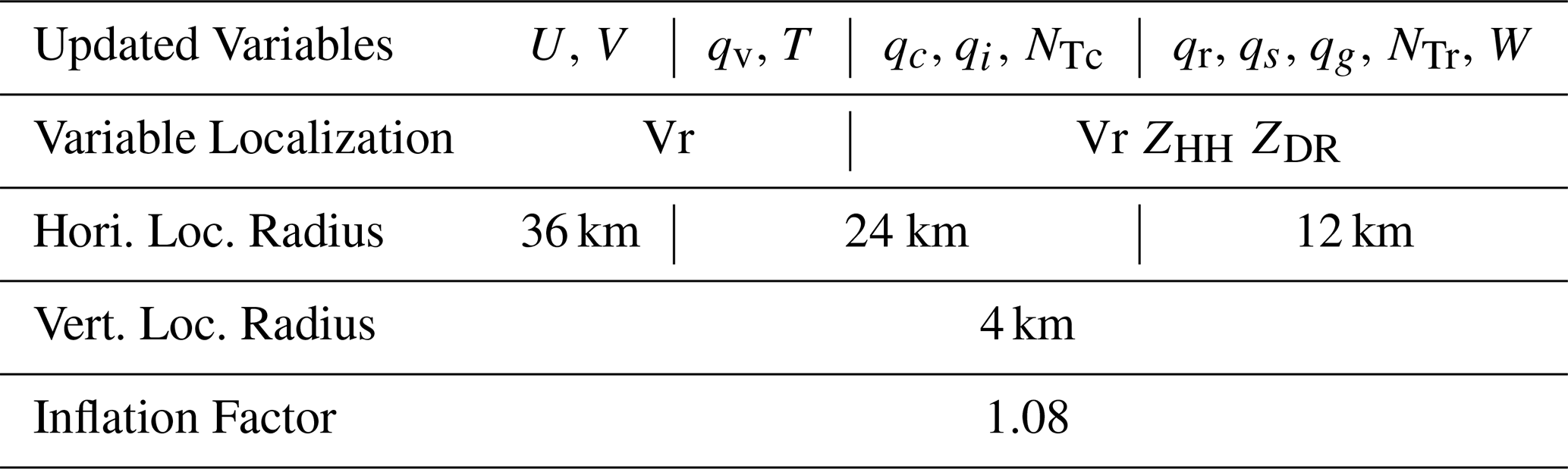
In this study, the employed configuration of the WLRAS system, including the localization radius and multiple inflation factors, is set on the basis of that used in You et al. (2020) and is presented in Table 1. The observation error standard deviation of the radial velocity, reflectivity, and differential reflectivity are considered to be 2 m s⁻¹, 5 dBZ (You et al., 2020), and 0.2 dB (Jung et al., 2008b), respectively. Variable localization is conducted when assimilating different observed parameters into the model. Finally, the super-observation method is performed on each elevation to prevent overfitting during assimilation. The resolution in the super-observation method is 2 km and 2°, and this method is applied at each observed elevation.

Table 1 Configuration of the WLRAS.

2.2 Observation Operator

Since dual-polarization parameters cannot be prognosticated by a numerical model, variables must be transformed before calculating the error covariance and the innovation. To directly assimilate radar data without variable retrieval, the observation operator can transform the prognostic variables into simulated radar variables on the basis of observation theories. In this study, the observation operators of the radial velocity and dual-polarization parameters are implemented; these operators are described in the following subsections.

2.2.1 Radial velocity observation operator

The observation operator of the radial velocity considers three-dimensional wind and hydrometeor terminal velocity. The following formula is used for calculating the radial velocity:

$$\begin{array}{}\text{(5)}& V_{\mathrm{r}}={\displaystyle \frac{Ux+Vy+(W-V_{\mathrm{t}})z}{(x^{\mathrm{2}}+y^{\mathrm{2}}+z^{\mathrm{2}}{)}^{\mathrm{0.5}}}}\end{array}$$

where U, V, and W are the three-dimensional wind components, and x, y, and z represent the three-dimensional components of the distance between particle and radar in Cartesian coordinates. The raindrop terminal velocity (V_t) is also included in calculating the radial velocity; the relevant formula is as follows:

$$\begin{array}{}\text{(6)}& V_{\mathrm{t}}=\mathrm{5.4}({\mathit{\rho }}_{\mathrm{a}}{q}_{\mathrm{r}}{)}^{\mathrm{0.125}}{\left({\displaystyle \frac{p_{\mathrm{0}}}{\stackrel{\mathrm{‾}}{p}}}\right)}^{\mathrm{0.4}}\end{array}$$

where ρ_a is the density of air; q_r is the rainwater mixing ratio, and p₀ is the surface pressure. Furthermore, $\stackrel{\mathrm{‾}}{p}$ is the average pressure in a certain layer and is used to calculate V_t at different altitudes.

2.2.2 Dual-polarization observation operator

In this study, the dual-polarization observation operator based on polarimetric radar data simulator (PRDS; Jung et al., 2008a, 2010) is implemented. The following equations reveal the configuration of the operator. First, the horizontal and vertical reflectivity factors (Z_h,x and Z_v,x) of each hydrometeor species are derived by Eqs. (7) and (8):

$$\begin{array}{}\text{(7)}& {\displaystyle }\begin{array}{rl}{Z}_{\mathrm{h},x}={\displaystyle \frac{\mathrm{4}{\mathit{\lambda }}^{\mathrm{4}}}{{\mathit{\pi }}^{\mathrm{4}}|K_{\mathrm{w}}{|}^{\mathrm{2}}}}\int & N_x\left(D\right)\left(A\right|f_{\mathrm{h},x}\left(\mathit{\pi }\right){|}^{\mathrm{2}}+B\left|f_{\mathrm{v},x}\right(\mathit{\pi }){|}^{\mathrm{2}}\\ & +\mathrm{2}C\left|f_{\mathrm{h},x}\right(\mathit{\pi }\left)\right|\left|f_{\mathrm{v},x}\right(\mathit{\pi }\left)\right|)\mathrm{d}D\end{array}\text{(8)}& {\displaystyle }\begin{array}{rl}{Z}_{\mathrm{v},x}={\displaystyle \frac{\mathrm{4}{\mathit{\lambda }}^{\mathrm{4}}}{{\mathit{\pi }}^{\mathrm{4}}|K_{\mathrm{w}}{|}^{\mathrm{2}}}}\int & N_x\left(D\right)\left(A\right|f_{\mathrm{v},x}\left(\mathit{\pi }\right){|}^{\mathrm{2}}+B\left|f_{\mathrm{h},x}\right(\mathit{\pi }){|}^{\mathrm{2}}\\ & +\mathrm{2}C\left|f_{\mathrm{h},x}\right(\mathit{\pi }\left)\right|\left|f_{\mathrm{v},x}\right(\mathit{\pi }\left)\right|)\mathrm{d}D\end{array}\end{array}$$

where N_x(D) is hydrometeor number concentration, and K_w is the dielectric factor of water; $\left|f_{\mathrm{h},x}\right(\mathit{\pi }\left)\right|$ and $\left|f_{\mathrm{v},x}\right(\mathit{\pi }\left)\right|$ are horizontal and vertical backscatter amplitude, respectively. The hydrometeor canting effect is described by the coefficients A, B and C, which are calculated using the following equations:

$$\begin{array}{}\text{(9)}& {\displaystyle }A={\displaystyle \frac{\mathrm{1}}{\mathrm{8}}}(\mathrm{3}+\mathrm{4}\cos \mathrm{2}\stackrel{\mathrm{‾}}{\mathrm{\Phi }}{e}^{-\mathrm{2}{\mathit{\sigma }}^{\mathrm{2}}}+\cos \mathrm{4}\stackrel{\mathrm{‾}}{\mathrm{\Phi }}{e}^{-\mathrm{8}{\mathit{\sigma }}^{\mathrm{2}}})\text{(10)}& {\displaystyle }B={\displaystyle \frac{\mathrm{1}}{\mathrm{8}}}(\mathrm{3}-\mathrm{4}\cos \mathrm{2}\stackrel{\mathrm{‾}}{\mathrm{\Phi }}{e}^{-\mathrm{2}{\mathit{\sigma }}^{\mathrm{2}}}+\cos \mathrm{4}\stackrel{\mathrm{‾}}{\mathrm{\Phi }}{e}^{-\mathrm{8}{\mathit{\sigma }}^{\mathrm{2}}})\text{(11)}& {\displaystyle }C={\displaystyle \frac{\mathrm{1}}{\mathrm{8}}}(\mathrm{1}-\mathrm{4}\cos \mathrm{4}\stackrel{\mathrm{‾}}{\mathrm{\Phi }}{e}^{-\mathrm{8}{\mathit{\sigma }}^{\mathrm{2}}})\end{array}$$

where $\stackrel{\mathrm{‾}}{\mathrm{\Phi }}$ is the mean and σ is the standard deviation of the canting angle. Considering the scattering of mixed-phase particles, the PRDS establishes the mixing model with the fraction of ice particles and rainwater. Also, the characteristics of mixing particles, such as the canting motion and the scattering intensity, are described in the mixing model. The coefficients and formula of the mixing-phase model are established as they are in You et al. (2020) and Jung et al. (2008a). Finally, the reflectivity and differential reflectivity in decibel scale can be obtained from the combination of reflectivity factors of all hydrometeor species as follows:

$$\begin{array}{}\text{(12)}& {\displaystyle }{Z}_{\text{HH}}={\log }_{\mathrm{10}}(\sum Z_{\mathrm{h},x})\text{(13)}& {\displaystyle }{Z}_{\text{VV}}={\log }_{\mathrm{10}}(\sum Z_{\mathrm{v},x})\text{(14)}& {\displaystyle }{Z}_{\text{DR}}={\log }_{\mathrm{10}}(\sum Z_{\mathrm{h},x}/\sum Z_{\mathrm{v},x})\end{array}$$

2.2.3 Scattering amplitude inside the observation operator

In Eqs. (7) and (8), the reflectivity factor can be derived by integrating total number concentrations and the backscattering amplitude with respect to diameter. To calculate the scattering amplitude, previous studies utilized T-matrix scattering calculations (Vivekanandan et al., 1991) before simulating the dual-polarization parameters. The T-matrix method considers the impact of the canting motion and the environment on electrometric wave transmission to ensure the simulation is as real as possible. The setting of environmental parameters, including the background temperature and density of hydrometeor species, may lead to different refraction characteristics. In addition, the particle axis ratio is fixed for each hydrometeor species to describe the characteristic scattering caused by the shape of the hydrometeors. A look-up table, which records the scattering amplitude for different diameter intervals, can be created from the results of single-particle simulation by using the T-matrix method. The reflectivity factors can then be derived using Eqs. (7) and (8). Many of the operators have a similar framework (Pfeifer et al., 2008; Jung et al., 2010; Ryzhkov et al., 2011; Augros et al., 2016, 2018; Oue et al., 2020). Although the integration method may yield dual-polarimetric parameters with reasonable structure, its computational cost is inevitably high. To decrease this cost, analytic equations are used in some operators to replace the integration (Zhang et al., 2001; Jung et al., 2008a; Kawabata et al., 2018). In these operators, the scattering amplitude is described as a function of drop size with assumptions, such as the function form of the hydrometeor axis ratio. Additionally, using the bulk microphysics scheme, the DSD can be described by gamma function parameters [the intercept, shape, and slope parameter in Eq. (1)]. This approach simplifies the calculation because integration does not need to be performed over the entire diameter interval.

In this study, the main structure of the operator is based on Jung et al. (2008a), which uses an analytic function to obtain the dual-polarimetric parameters. To fit the relationship between the particle diameter and scattering amplitude, the power-law function is applied as follows:

$$\begin{array}{}\text{(15)}& {\displaystyle }\left|f_{\mathrm{h}}\right|={\mathit{\alpha }}_{\mathrm{h},x}{D}_x^{{\mathit{\beta }}_{\mathrm{h},x}}\text{(16)}& {\displaystyle }\left|f_{\mathrm{v}}\right|={\mathit{\alpha }}_{\mathrm{v},x}{D}_x^{{\mathit{\beta }}_{\mathrm{v},x}}\end{array}$$

where D is the diameter of a hydrometer species and α_h,x, α_v,x, β_h,x, and β_v,x, are fitting coefficients that are set to those used in You et al. (2020) and Jung et al. (2008a). Substituting the fitting coefficients and assumed the gamma-shaped DSD into Eqs. (6) and (7) yields the following equations:

$$\begin{array}{}\text{(17)}& {\displaystyle }\begin{array}{rl}{Z}_{\mathrm{h},x}& ={\displaystyle \frac{\mathrm{4}{\mathit{\lambda }}^{\mathrm{4}}{N}_{\mathrm{0},x}}{{\mathit{\pi }}^{\mathrm{4}}|K_{\mathrm{w}}{|}^{\mathrm{2}}}}(A{\mathit{\alpha }}_{\mathrm{h},x}^{\mathrm{2}}{\displaystyle \frac{\mathrm{\Gamma }({\mathit{\mu }}_x+\mathrm{2}{\mathit{\beta }}_{\mathrm{h},x}+\mathrm{1})}{{\mathrm{\Lambda }}_x^{{\mathit{\mu }}_x+\mathrm{2}{\mathit{\beta }}_{\mathrm{h},x}+\mathrm{1}}}}\\ & +B{\mathit{\alpha }}_{\mathrm{v},x}^{\mathrm{2}}{\displaystyle \frac{\mathrm{\Gamma }({\mathit{\mu }}_x+\mathrm{2}{\mathit{\beta }}_{\mathrm{v},x}+\mathrm{1})}{{\mathrm{\Lambda }}_x^{{\mathit{\mu }}_x+\mathrm{2}{\mathit{\beta }}_{\mathrm{v},x}+\mathrm{1}}}}\\ & +\mathrm{2}C{\mathit{\alpha }}_{\mathrm{h},x}{\mathit{\alpha }}_{\mathrm{v},x}{\displaystyle \frac{\mathrm{\Gamma }({\mathit{\mu }}_x+{\mathit{\beta }}_{\mathrm{h},x}+{\mathit{\beta }}_{\mathrm{v},x}+\mathrm{1})}{{\mathrm{\Lambda }}_x^{{\mathit{\mu }}_x+{\mathit{\beta }}_{\mathrm{h},x}+{\mathit{\beta }}_{\mathrm{v},x}+\mathrm{1}}}})\end{array}\text{(18)}& {\displaystyle }\begin{array}{rl}{Z}_{\mathrm{v},x}& ={\displaystyle \frac{\mathrm{4}{\mathit{\lambda }}^{\mathrm{4}}{N}_{\mathrm{0},x}}{{\mathit{\pi }}^{\mathrm{4}}|K_{\mathrm{w}}{|}^{\mathrm{2}}}}(A{\mathit{\alpha }}_{\mathrm{v},x}^{\mathrm{2}}{\displaystyle \frac{\mathrm{\Gamma }({\mathit{\mu }}_x+\mathrm{2}{\mathit{\beta }}_{\mathrm{v},x}+\mathrm{1})}{{\mathrm{\Lambda }}_x^{{\mathit{\mu }}_x+\mathrm{2}{\mathit{\beta }}_{\mathrm{v},x}+\mathrm{1}}}}\\ & +B{\mathit{\alpha }}_{\mathrm{h},x}^{\mathrm{2}}{\displaystyle \frac{\mathrm{\Gamma }({\mathit{\mu }}_x+\mathrm{2}{\mathit{\beta }}_{\mathrm{h},x}+\mathrm{1})}{{\mathrm{\Lambda }}_x^{{\mathit{\mu }}_x+\mathrm{2}{\mathit{\beta }}_{\mathrm{h},x}+\mathrm{1}}}}\\ & +\mathrm{2}C{\mathit{\alpha }}_{\mathrm{h},x}{\mathit{\alpha }}_{\mathrm{v},x}{\displaystyle \frac{\mathrm{\Gamma }({\mathit{\mu }}_x+{\mathit{\beta }}_{\mathrm{h},x}+{\mathit{\beta }}_{\mathrm{v},x}+\mathrm{1})}{{\mathrm{\Lambda }}_x^{{\mathit{\mu }}_x+{\mathit{\beta }}_{\mathrm{h},x}+{\mathit{\beta }}_{\mathrm{v},x}+\mathrm{1}}}})\end{array}\end{array}$$

The shape parameters (μ) of different hydrometeor species are fixed using the same configuration as that in the WRF double-moment 6-class (WDM6) MP scheme (Lim and Hong, 2010). The slope parameter (Λ) and intercept parameter (N₀) can be estimated using the following equations:

$$\begin{array}{}\text{(19)}& {\displaystyle }{\mathrm{\Lambda }}_x={\left[{\displaystyle \frac{\mathit{\pi }{\mathit{\rho }}_x{N}_{\mathrm{T},x}\mathrm{\Gamma }({\mathit{\mu }}_x+\mathrm{4})}{\mathrm{6}{\mathit{\rho }}_{\mathrm{a}}{q}_x\mathrm{\Gamma }({\mathit{\mu }}_x+\mathrm{1})}}\right]}^{\frac{\mathrm{1}}{\mathrm{3}}}\text{(20)}& {\displaystyle }{N}_{\mathrm{0},x}={\displaystyle \frac{{\mathrm{\Lambda }}_x^{{\mathit{\mu }}_x+\mathrm{1}}{N}_{\mathrm{T},x}}{\mathrm{\Gamma }({\mathit{\mu }}_x+\mathrm{1})}}\end{array}$$

where ρ_a is the density of air; ρ_x is the density of hydrometeor species in the corresponding setting of the MP scheme. q_x and N_T,x are the predicted mixing ratio and total number concentration of hydrometeor species, respectively. Finally, by using Eqs. (17) and (18), the reflectivity factor can be derived without integration. The details of the configuration in the PRDS are described in Jung et al. (2008a).

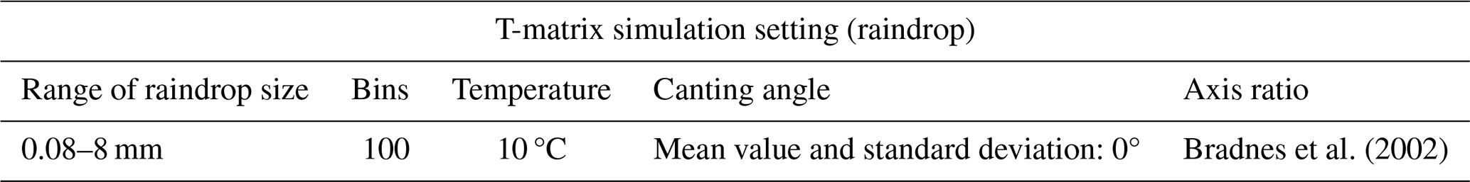
The direct integration method can also be employed in calculating the raindrop-contributed reflectivity factor and is compared with the power-law fitting method in this study. The T-matrix method is applied to simulate the scattering amplitude with respect to different raindrop sizes. The environmental conditions of the T-matrix simulation, including temperature, canting angle, and drop size bin intervals, are set on the basis of the setting in Jung et al. (2010) and are presented in Table 2. Finally, the factors of the raindrop-contributed reflectivity factors on both axes are derived by directly integrating the raindrop number concentration and scattering amplitude with respect to the drop size diameter.

Table 2 Configuration of the T-matrix scattering simulation.

3 Data and Case Overview

3.1 Case Overview

In this study, real case data assimilation experiments on summertime rainfall events are conducted to evaluate the influence of the employed specific operator configuration. Three cases are selected, including a squall line case, a typhoon case and a Mei-Yu frontal case (stationary frontal case), to validate the simulations for various weather types.

3.1.1 Squall line case

Located near the boundary of Eurasia and the Pacific Ocean, Taiwan has the weather system that is strongly affected by the moisture in air transported by the East Asia monsoon, especially in terms of its summertime rainfall. This study selects the case of squall line on 14 June 2008, during the eighth intensive observation period of the Southwest Monsoon Experiment (SoWMEX-IOP8). In this period, the southeastern Asian monsoon low drove a southerly wind near Taiwan and propagated moist air from the Indian Ocean to the South China Sea and Taiwan Strait, creating an environment favorable for system development (Fig. 1a, b). Therefore, several mesoscale systems, including the squall line system, developed and impacted southern Taiwan, causing more than 300 mm of rainfall over three days (Lupo et al., 2020). At 12:00 UTC on 14 June 2008, the squall line system was well developed and impacted southern Taiwan (Fig. 1c). As revealed by the National Center of Atmospheric Research (NCAR) S-band dual-polarimetric radar (S-POL) observation, Z_HH extended to higher than 45 dBZ, and Z_DR was mainly within 0–1 dB (Fig. 1d). Thus, the strong rainfall system mainly comprised small raindrops.

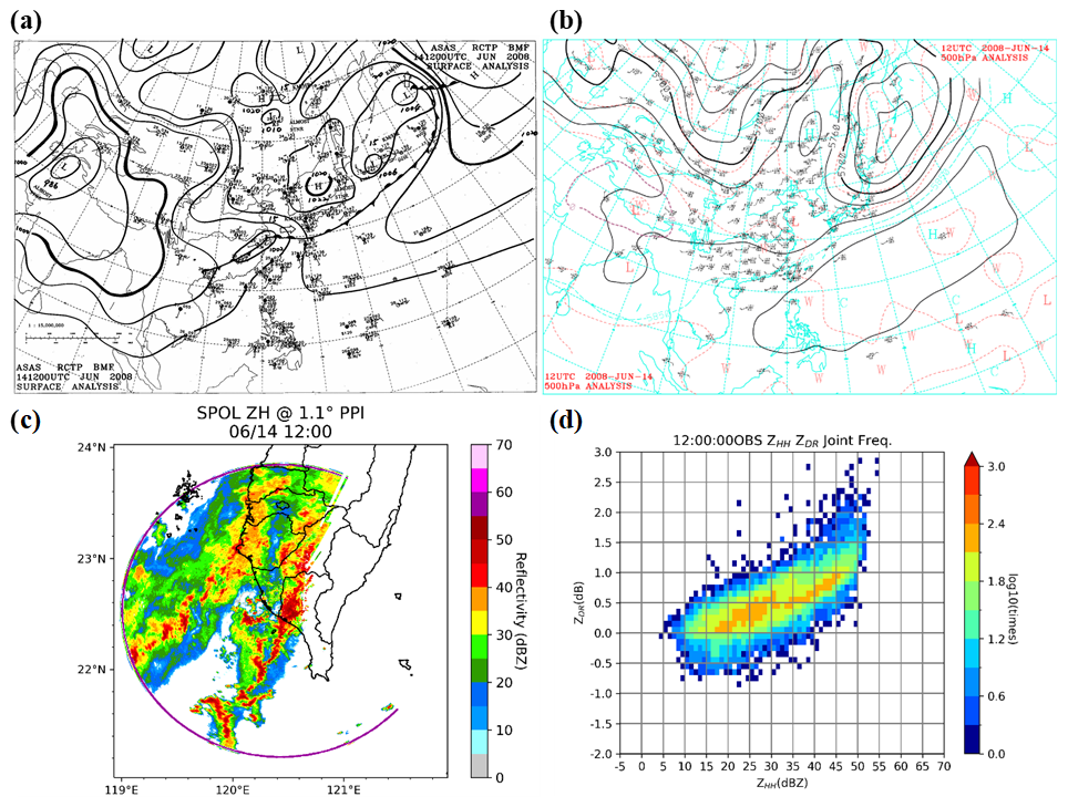
Figure 1 Synoptic-scale and meso-scale observations of the SoWMEX IOP8 squall line case at 12:00 UTC on 14 June 2008. Synoptic-scale: (a) surface weather map and (b) 500 hPa analyses weather map from the Central Weather Administration (CWA). Meso-scale: (c) reflectivity at 1.1° elevation, observed by SPOL, and (d) Z_HH–Z_DR joint frequency.

3.1.2 Typhoon case

During summer and autumn, Taiwan is frequently struck by typhoons. On average, approximately three typhoons affect the island each year. They bring destructive winds and considerable rainfall, often destroying the landscape and leading to severe flooding. Therefore, studies of typhoons is crucial for Taiwan. In this study, a violent typhoon, Typhoon Soudelor, is selected as the research target to validate the impact of dual-polarization data assimilation. Typhoon Soudelor affected Taiwan from 7 to 9 August 2015 (Fig. 2a, b), and caused more than 300 mm of rainfall during this period. Some places, particularly mountainous regions, received more than 600 mm of rainfall. Considerable damage was caused by the typhoon, including flooding and landslides in northern Taiwan. Furthermore, a record-breaking gust of wind devastated the electric power system, leading to the largest blackout on record in Taiwan. The radar observation made by the Wufenshan Weather Radar Station (RCWF) indicated that an intense rain band of more than 45 dBZ directly struck northeastern Taiwan and resulted in heavy rainfall (Fig. 2c). The high occurrence frequency of Z_HH extended to 45 dBZ, and Z_DR was mainly within 0.5–1.3 dB, indicating that the rain band mainly comprised small raindrops but larger drops than those in the squall line case and Mei-Yu frontal case (Fig. 2d).

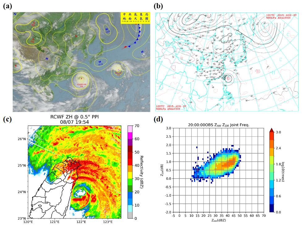
Figure 2 Synoptic-scale and meso-scale observations of the Typhoon Soudelor case. Synoptic scale: (a) surface weather map and (b) 500 hPa analyses weather map at 12:00 UTC on 7 August 2015, from Central Weather Administration (CWA). Meso scale: (c) reflectivity at 0.5° elevation observed by RCWF, at 19:54 UTC and (d) Z_HH–Z_DR joint frequency at 20:00 UTC on 7 August 2015.

3.1.3 Mei-Yu (stationary frontal MCS) case

The East Asia rainy season, also referred to as the Mei-Yu season, typically occurs during the early summer in middle-eastern Asia and late summer in northeastern Asia. The quasi-stationary front caused by cold and dry air from the north and warm and moist air from the south leads to an unstable environment, inducing an intense mesoscale convective system and sustained rainfall. The frontal system on 6 June 2022, during the third intense observation period of the Taiwan-Area Heavy Rain Observation and Prediction Experiment (TAHOPE) is selected in this study (Fig. 3a, b). The frontal system coupled with the low-level moisture environment gradually approached Taiwan, and a linear convective precipitation system was located in the north of Taiwan at 08:00 UTC (Fig. 3c). Radar observation by NCAR SPOL and RCWF indicated that the high occurrence frequency of Z_HH extended to 40 dBZ, and that Z_DR was mainly within 0.5–1.0 dB, indicating that the rain band was mainly comprised of raindrops (Fig. 3d).

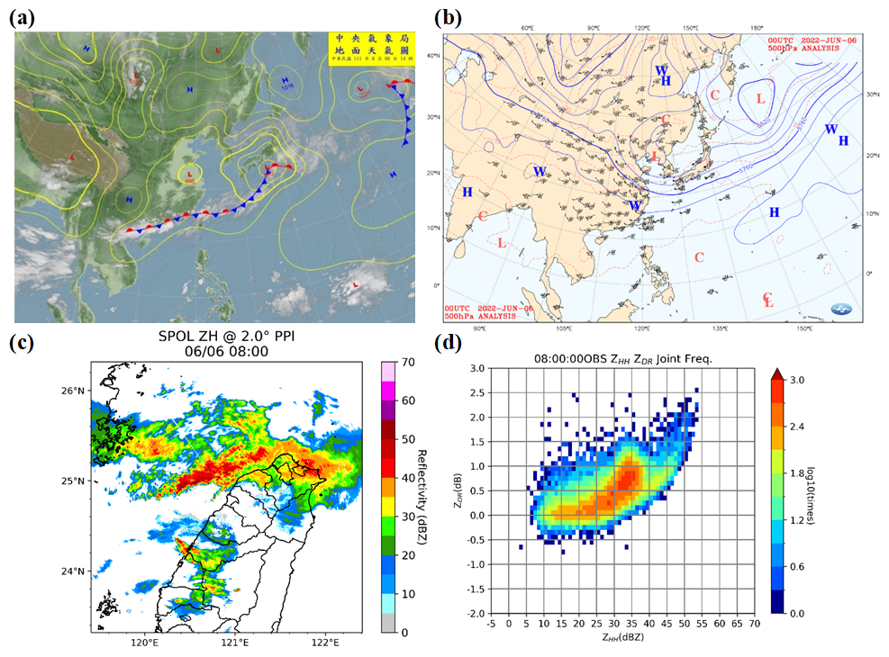
Figure 3 Synoptic-scale and meso-scale observations of the TAHOPE IOP3 Mei-Yu frontal case. Synoptic-scale: (a) surface weather map and (b) 500 hPa analyses weather map at 00:00 UTC on 6 June 2022, from the Central Weather Administration (CWA). Meso-scale: (c) reflectivity at 2.0° elevation observed by SPOL and (d) Z_HH–Z_DR joint frequency at 08:00 UTC on 6 June 2022.

3.2 Radar Data Quality Control

In this study, the radar data from NCAR SPOL and operational S-band weather radars – RCWF (Wufengshan Radar Weather Station), RCKT (Kenting Radar Weather Station), RCHL (Hualien Radar Weather Station), and RCCG (Chigu Radar Weather Station) – are assimilated into the model (Fig. 4). Since the radar observation network has gradually updated from single-polarization to dual-polarization radar, the observed parameters and the scanning strategies of radars are different in three cases. In the SoWMEX IOP8 squall line case, all operational radars had the same scanning strategies: nine elevation angles (0.5, 1.4, 2.4, 3.4, 4.3, 6.0, 9.9, 14.6 and 19.5°) and provided single-pol Doppler radar parameters, the reflectivity (Z_HH) and radial wind (Vr). For the cases after 2015, the same strategies were used for most radars, although RCWF was updated to dual-polarization weather radar, providing operational dual-polarization radar data with 15 elevation angles in the one volume scan (0.5, 0.9, 1.3, 1.8, 2.4, 3.1, 4.0, 5.1, 6.4, 8.0, 10.0, 12.0, 14.0, 16.7, and 19.5°). NCAR SPOL data were used in the 2008 SoWMEX and 2022 TAHOPE, and the radar provides dual-polarization data. SPOL scanned with 9 elevation angles (0.5, 1.1, 1.8, 2.6, 3.6, 4.7, 6.5, 9.1 and 12.8°) in 2008 and 10 elevation angles (0.5, 1.0, 1.5, 2.0, 3.0, 4.0, 5.0, 7.0, 9.0 and 11.0°) in 2022, providing substantial data regarding the nearby surface, and therefore, the structure of the intense rainfall system could be comprehensively studied.

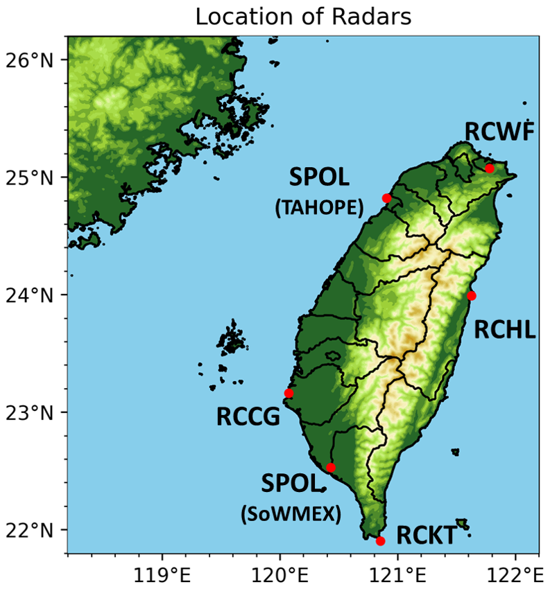
Figure 4 Location of the SPOL and operational radars in Taiwan.

A quality control process is used to prevent the model from being contaminated by non-meteorological signals. On the basis of the characteristics of dual-polarization radar parameters, certain thresholds are employed to remove noise. The Radar Kit (Rakit) developed by National Central University is employed to control the quality of the radar data. Single-polarization radar data are first corrected by terrain height to avoid the radar beam being blocked; then, the radial velocity is unfolded and used to remove the non-meteorological signal in accordance with a certain threshold: Z_HH>30 dBZ and Vr<2 m s⁻¹. For the dual-polarization radars, in the first step of quality control, Φ_dp at different elevations is unfolded. Subsequently, ρ_hv>0.9 and Φ_dp standard deviation <10 are applied to filter out non-meteorological noise. In addition, the radial velocity would be unfolded. Finally, the Z_DR systematic bias of RCWF is calculated by the mean value of Z_DR observation at the low-reflectivity (15–25 dBZ) region using the method mentioned in Loh et al. (2022).

4 Configuration of Model and Experiments

4.1 Model Configuration

In this study, Weather Research and Forecasting (WRF) version 3.9.1 is applied to simulate the summertime rainfall events and to conduct radar data assimilation. WRF model is a nonhydrostatic and compressible regional numerical model coupled with various types of physics parameterizations that is suitable to simulate the complex physics, dynamics and thermodynamics mechanisms behind the mesoscale weather system. Focus on the area nearby Taiwan, three nested domains are employed from large scale, covering the eastern Asia, to the small scale, covering nearby Taiwan. For each domain, the top of the model is set at 10 hPa height with 52 η levels, and the horizontal resolution is 15, 3, and 1 km in the first, second, and third domain (D01–D03), respectively (Fig. 5). To obtain a reasonable synoptic-scale structure, NCEP FNL operational model global tropospheric analyses with 0.25° resolution are used to generate the initial and boundary conditions. Four physics parameterization schemes are used to represent the sub-grid physical processes, including Dudhia short-wave radiation parameterization scheme (Dudhia, 1989), Rapid Radiative Transfer Model (RRTM) longwave radiation parameterization scheme (Mlawer et al., 1997), Yonsei University (YSU) planetary boundary layer parameterization scheme (Hong et al., 2006), and Grell-Freitas cumulus parameterization scheme (Grell and Dévényi 2002; only in D01). Moreover, the WDM6 MP scheme (Lim and Hong, 2010) is implemented to evolve the performance of the microphysics processes and provide prognostic variables including the mixing ratio of the rain, water vapor, cloud droplets, ice and graupel/hail, and the total number concentration of the rain and cloud droplets. To conduct EnKF data assimilation, ensemble forecasts with 50 members are generated. For each member, the horizontal wind field, perturbation potential temperature, and water vapor in D01 are perturbed using the WRFDA cv3 option; then, the perturbed initial condition would soon be downscaled to the nested domains after perturbation. For all of the cases, the simulation would be initialized and spun up before the first DA cycle.

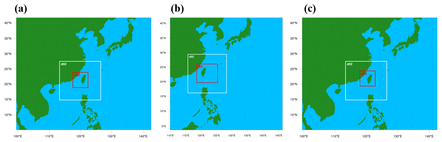
Figure 5 Configuration of nested domains in (a) SoWMEX IOP8 squall line case, (b) Typhoon Soudelor case, and (c) TAHOPE IOP3 Mei-Yu frontal case with 15, 3, and 1 km horizontal resolution in D01, D02, and D03 respectively.

4.2 Experiment Design

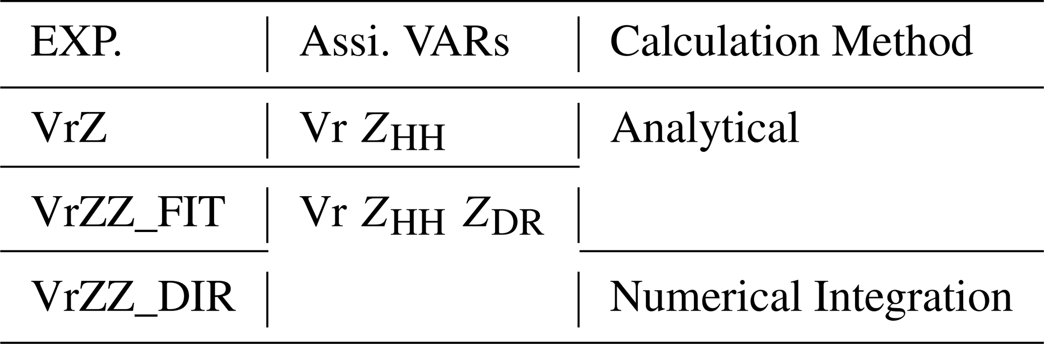
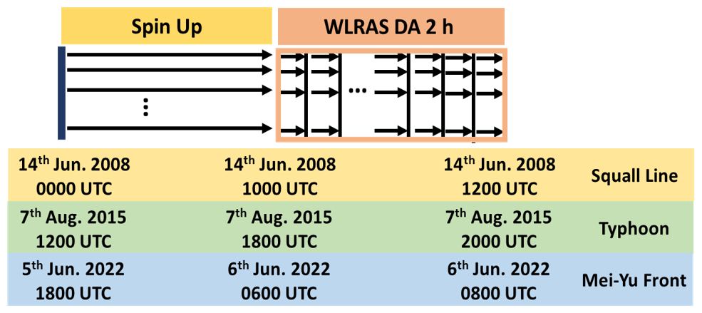
Three experiments are conducted in this study (Table 3). In the VrZ experiment, only Z_HH and V_r are assimilated, which is used to validate the background performance when Z_DR is not assimilated into model. In the VrZZ_FIT experiment, Z_HH, V_r and Z_DR are assimilated using the fitting method inside the operator. In the VrZZ_DIR experiment, the same variables are assimilated but the direct integration method is used to calculate the raindrop-contributed reflectivity factor. The DA procedure in the three cases is illustrated in Fig. 6, including the model spin-up and 2 h DA window. The period of each DA cycle is 15 min in the squall line and the typhoon case, but 12 min in the Mei-Yu frontal case because more rapid scanning is available in that event. In each cycle, the dual-polarization radar data are assimilated in the following order: (1) Vr, (2) Z_HH, and (3) Z_DR. Finally, only Z_DR observations below 4 km are assimilated, which is below the melting layer in the model and observation, and this is performed to specifically focus on the impact of using different calculation methods on the raindrop-contributed term.

Table 3 Experimental design.

Figure 6 Flowchart of the assimilation procedure.

5 Results and Discussions

5.1 Performance of Simulated Variables

The background error covariance between the assimilated variables and state variables is strongly affected by the configurations inside the forward operators. Also, the innovation, which indicates the direction of the model updating, may be incorrect when the simulation has some bias caused by the model and forward operator. Therefore, the performance of the forward operator must be evaluated before data assimilation. In this study, the simulated dual-polarization radar parameters in the background are validated by observation data. Figure 7 presents the overall performance of the analyzed dual-polarization radar parameters in experiment VrZ below 4 km when two operators are used to transform the variables. The results reveal that both operators capture the structure of reflectivity, in which the mean difference between simulation and observation is less than 5 dBZ for the whole period. The results obtained using different calculation methods are in strong agreement, indicating that the fitting method successfully simulates reflectivity while consuming fewer computational resources, which only cost one-fifth of the computational resources. However, the simulated Z_DR using the fitting method operator differs considerably from observation, and the uncertainty is higher than that in the VrZ_DIR experiment and the observation. Additionally, the negative Z_DR is simulated through the fitting method in the Mei-Yu frontal case, and considerable positive bias occurs in the typhoon case. By contrast, directly deriving the dual-polarization parameters through numerical integration not only captures the Z_HH structure but also yields a reasonable Z_DR in the VrZ experiment, leading to much more Z_DR data being assimilated under the same innovation threshold of the DA (Fig. 8).

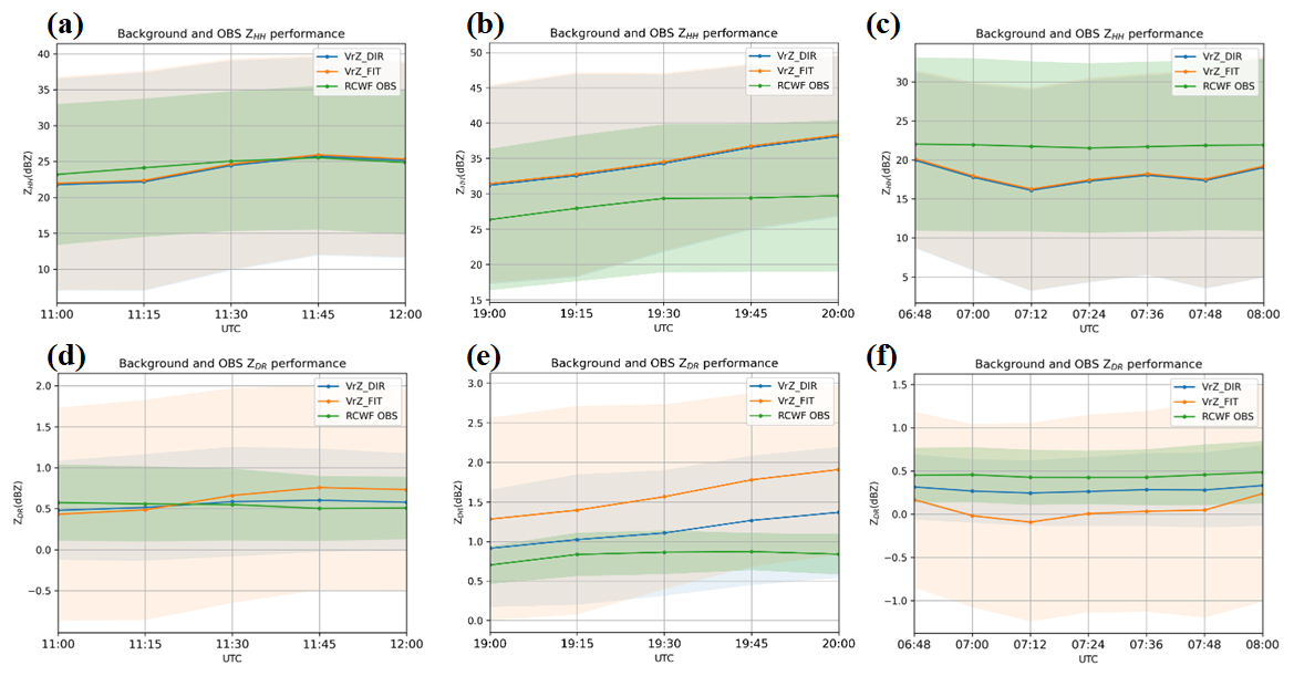
Figure 7 Overall performance of (a–c) reflectivity and (d–f) Z_DR below 4 km in the VrZ analyses and dual-polarization radar observation in the (a, d) squall line case, (b, e) typhoon case and (c, f) Mei-Yu frontal case. Solid line: mean value of the data; shaded region: within one standard deviation. Blue and orange respectively indicate the VrZ performance when the fitting method and direct integration method are used; green color indicates the observations.

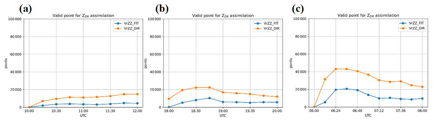
Figure 8 Valid points for Z_DR assimilation calculated in VrZ analyses when different operators are used in the (a) squall line case, (b) typhoon case, and (c) Mei-Yu frontal case. Blue and orange respectively indicates the performance when the fitting method and direct integration method are used.

Since the validation mainly focuses on the region below the melting layer, which is dominated by liquid-phase particles, the presence of a negative value is unexpected. The reason for the Z_DR negative value can be determined from Eqs. (17) and (18). If we only focus on the raindrop's contribution to the reflectivity, the Eqs. (17) and (18) could be written as follows:

$$\begin{array}{}\text{(21)}& \begin{array}{rl}{Z}_{\text{DR,rain}}& =\mathrm{10}{\log }_{\mathrm{10}}\left({\displaystyle \frac{Z_{\text{h,rain}}}{Z_{\text{v,rain}}}}\right)\\ & \begin{array}{rl}=\mathrm{10}{\log }_{\mathrm{10}}(& {\displaystyle \frac{\mathrm{\Gamma }(\mathrm{2}{\mathit{\beta }}_{r,\mathrm{h}}+\mathit{\mu }+\mathrm{1})}{\mathrm{\Gamma }(\mathrm{2}{\mathit{\beta }}_{r,\mathrm{v}}+\mathit{\mu }+\mathrm{1})}}\times \\ & {\mathrm{\Lambda }}^{\left[\right(\mathrm{2}{\mathit{\beta }}_{r,\mathrm{h}}+\mathit{\mu }+\mathrm{1})-(\mathrm{2}{\mathit{\beta }}_{r,\mathrm{v}}+\mathit{\mu }+\mathrm{1}\left)\right]})\end{array}\end{array}\end{array}$$

Subsequently, when the fitting coefficients mentioned by Jung et al. (2008a) are used, β_r,h and β_r,v are 3.04 and 2.77, respectively. Substituting these coefficients and the shape parameter of raindrops in WDM6 (μ=1) into Eq. (21) yields the following:

$$\begin{array}{}\text{(22)}& \begin{array}{rl}{Z}_{\text{DR,rain}}& \approx \mathrm{10}{\log }_{\mathrm{10}}(\mathrm{2.928}{\mathrm{\Lambda }}^{-\mathrm{0.54}}\times {\mathrm{10}}^{\mathrm{1.62}})\\ & \approx \mathrm{10}{\log }_{\mathrm{10}}\left(\mathrm{122.08}{\mathrm{\Lambda }}^{-\mathrm{0.54}}\right)\end{array}\end{array}$$

Due to the law of the logarithm, when Λ^0.54>122.08, Z_DR,rain may be less than 0, leading to the unreasonable negative Z_DR,rain value in the simulation. The same result may be obtained for other operators when the power-law function is used to describe the relationship between scattering amplitude and drop size. Hence, before applying the forward operator to simulate the dual-polarization radar parameters, the properties of the operator should be considered to ensure the simulation is reasonable in the given interval of the drop size.

5.2 Validation of Dual-Polarization Parameters

This section presents the validation of simulated variables from the LETKF forecasts and analyses. Figure 9 shows the observed and analyzed reflectivity at the final analysis time. Compared with the observations, both experiments successfully reproduce the overall structure of the precipitation systems after assimilating dual-polarization radar data and exhibit similar performance across the three cases. However, both experiments slightly underestimate the intensity of the system, particularly in the squall-line case and in the VrZZ_FIT experiment for the typhoon case. In contrast to reflectivity, the analyzed Z_DR exhibits more distinct differences between the two experiments (Fig. 10). Compared with the observation, VrZZ_DIR has a reasonable Z_DR distribution and is able to capture the main structural features of the system, although the Z_DR intensity is still overestimated in the Mei-Yu frontal case. By comparison, VrZZ_DIR experiment shows poorer performance in simulating Z_DR failing to adequately represent its intensity, with overestimated extreme values and underestimated Z_DR in the surrounding regions of the system. To quantitative evaluate the model, the difference between observation and simulation data, root mean square residual (RMSR), is calculated as follows:

$$\begin{array}{}\text{(23)}& \text{RMSR}=\sqrt{{\displaystyle \frac{\sum (y^{\mathrm{o}}-H{\stackrel{\mathrm{‾}}{x}}^{\mathrm{a}}{)}^{\mathrm{2}}}{n}}}\end{array}$$

The term inside the parentheses is the residual, which means the difference between observation and analyses in observation space. The closer the RMSE is to zero, the closer the simulation is to the observation. Figure 11 shows the Z_HH and Z_DR RMSR for the entire DA period. To estimate the impact of the raindrop-contributed term, the Z_DR RMSR is calculated with the observations below 4 km, which are the height lower than the melting layer in the observation and simulation. The Z_HH RMSR values determined for the two operator settings are similar in the three cases, and the difference between the VrZZ_DIR and VrZZ_FIT experiments is approximately 1.0–2.0 dBZ in all cases. However, the Z_DR RMSR indicates a considerable difference between two experiments that VrZZ_DIR has a lower residual compared to VrZZ_FIT. This result can be explained by two reasons: First, the direct integration method prevents negative Z_DR and yields a more similar Z_DR structure during DA cycling. Conversely, much more Z_DR observation information can be assimilated into the model and used to modify the simulation toward the observation when using the direct integration method. The difference joint frequencies calculated from analyses and observation below a height of 4 km (Fig. 12) indicates the similar performance that in the VrZZ_FIT experiment, Z_DR is obviously overestimated for the three cases. Some high-frequency difference is even greater than +0.6 dB or less than −0.6 dB, which exceeds the threshold of the assimilation that Z_DRcannot be assimilated. Corresponding results could be indicated by the Z_HH–Z_DR joint frequencies under a height of 4 km (Fig. 13). The occurrence frequency in the background shows that the slope of the high-frequency area in the VrZZ_FIT experiment is greater than the slope in the observation data. By contrast, the Z_HH–Z_DR joint frequency in the VrZZ_DIR experiment is much closer to the observation. Assimilating Z_DR into the model results in the frequency being adjusted toward the observed value in both experiments, but the adjustment in the VrZZ_DIR experiment is greater than the one in the VrZZ_FIT experiment. Moreover, because Z_DR is generally overestimated in the VrZZ_FIT background, the assimilation tends to reduce Z_DR, which further exacerbates the issue of unrealistically negative Z_DR values when Z_HH<30 dBZ. This result indicates that VrZZ_FIT is unable to adequately correct the Z_DR intensity in light rain regions.

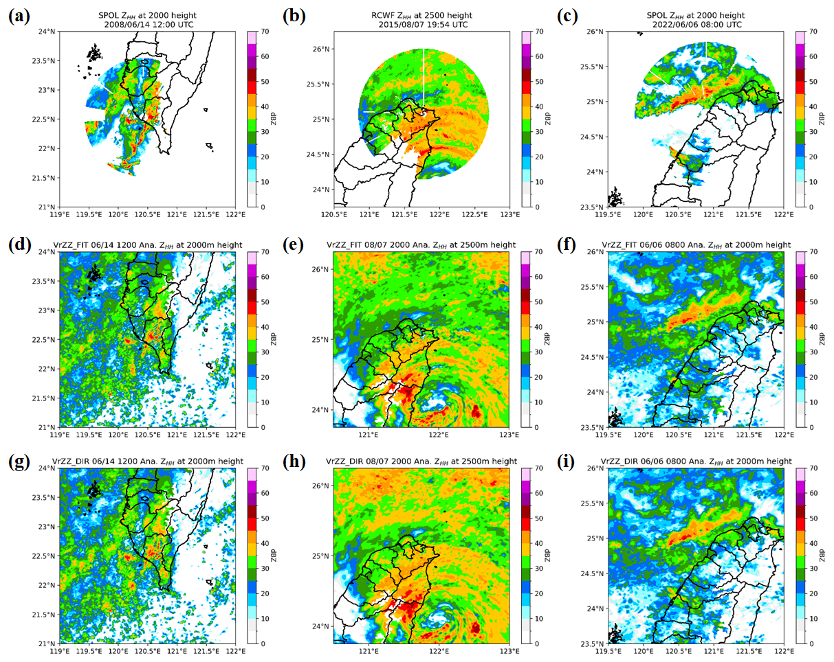
Figure 9 Analyzed Z_HH at the time of the final analyses in the (a–c) observation, (d–f) VrZZ_FIT, and (g–i) VrZZ_DIR for three cases: squall line (left column), typhoon (middle column) and Mei-Yu frontal case (right column).

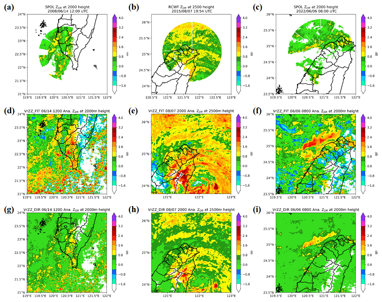
Figure 10 Analyzed Z_DR at the time of the final analyses in the (a–c) observation, (d–f) VrZZ_FIT, and (g–i) VrZZ_DIR for three cases: squall line (left column), typhoon (middle column) and Mei-Yu frontal case (right column).

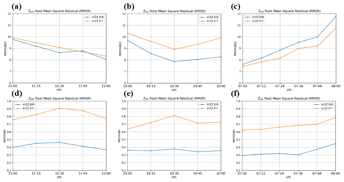
Figure 11 RMSR of (a–c) reflectivity and (d–f) Z_DR in the (a, d) squall line case, (b, e) typhoon case, and (c, f) Mei-Yu frontal case.

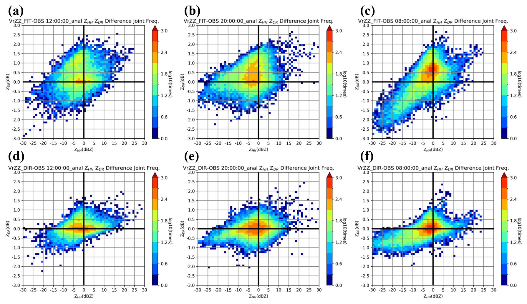
Figure 12 Z_HH–Z_DR difference joint frequency at the final analyses of the (a–c) VrZZ_FIT and (d–f) VrZZ_DIR experiments for the (a, d) squall line case, (b, e) typhoon case, and (c, f) Mei-Yu frontal case. The shading indicates the occurrence times of the difference calculated from the observation and simulation on the logarithmic scale. The horizontal and vertical axes are the Z_HH and Z_DR difference with 1 dBZ and 0.1 dB intervals, respectively.

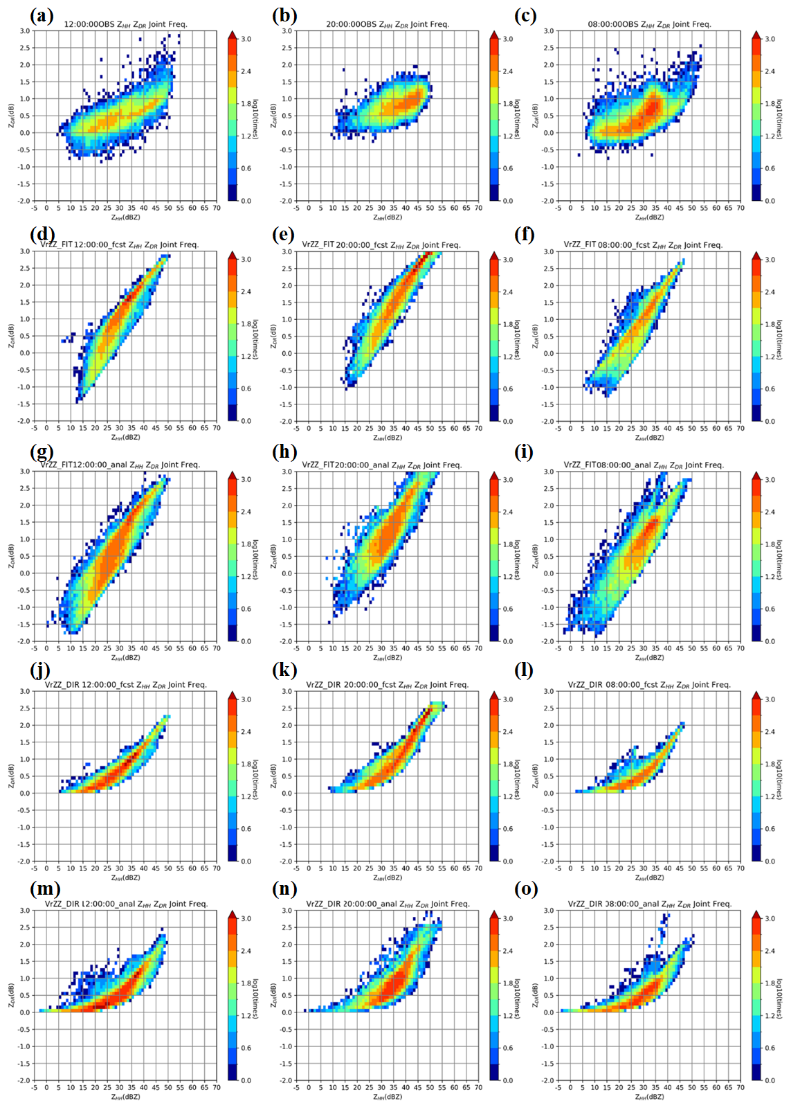
Figure 13 Z_HH–Z_DR joint frequency at the time of the final analyses in the (a–c) observation, (d–f) VrZZ_FIT background, (g–i) VrZZ_FIT analyses, (j–l) VrZZ_DIR background, and (m–o) VrZZ_DIR analyses for three cases: squall line (left column), typhoon (middle column) and Mei-Yu frontal case (right column). The shading is the occurrence times on the logarithmic scale. The horizontal and vertical axes are the Z_HH and Z_DR with 1 dBZ and 0.1 dB intervals, respectively.

Although the validations above suggest that the VrZZ_DIR experiment has a more reasonable simulation compared to the VrZZ_FIT experiment, there is still a difference between the VrZZ_DIR simulation and the observation. For instance, the occurrence frequency in the VrZZ_DIR experiment of Z_DR is overestimated for the typhoon case when Z_HH>30 dBZ. Besides, the joint frequency distribution in the VrZZ_DIR experiment is narrower than the one from observation data, indicating that the operator could not appropriately describe the degree of freedom in the observation. However, the Z_DR overestimation and narrow distribution in the VrZZ_DIR experiment could be modified after the assimilation, leading to a more reasonable structure compared with that obtained in the VrZZ_FIT. In sum, the clear difference in the Z_HH–Z_DR structure in the background limits the adjustment of assimilation in the VrZZ_FIT experiment, and the similar Z_HH–Z_DR structure in the VrZZ_DIR background leads to a more reasonable structure in the analyses.

5.3 Performance of Microphysics Structure

Since dual-polarization radar parameters are not prognostic variables, the adjustments of updated variables must be validated to determine how data assimilation affects the model. To evaluate the microphysics structure, this study uses the raindrop mass-weighted mean diameter (D_mr) retrieved from the dual-polarization radar observation as a reference observation. D_mr is obtained through the method reported by Cao et al. (2008) by using 15 years of disdrometer data observed at National Central University referenced by Lee et al. (2019). The result of fitting is as follows:

$$\begin{array}{}\text{(24)}& \begin{array}{rl}& D_{\text{mr}}=\\ & Z_{\text{HH}}(\mathrm{0.00946}{Z}_{\text{DR}}^{\mathrm{3}}-\mathrm{0.0277}{Z}_{\text{DR}}^{\mathrm{2}}+\mathrm{0.0323}{Z}_{\text{DR}}+\mathrm{0.0338})\end{array}\end{array}$$

Figures 14 and 15 present the D_mr–Z_DR occurrence joint frequency below 4 km height in the final cycle background and analyses, respectively. In all experiments, D_mr is underestimated in the background but is adjusted toward the observed value after dual-polarization radar assimilation. According to the comparison of the VrZZ_FIT and VrZZ_DIR experiments, the difference in D_mr between the two experiments is small, but the D_mr–Z_DR structure is more concentrated in the VrZZ_DIR findings because of the more correct Z_DR structure. Thus, when the method employed to calculate the raindrop-contributed term is changed, the characteristics of the raindrop prognostic variables do not change completely; however, the relationship between D_mr and Z_DR is more reasonable when the direct integration method is employed.

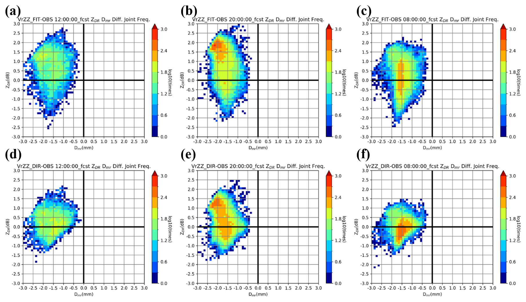
Figure 14 Background D_mr–Z_DR joint frequency at the time of the final analyses in the (a–c) VrZZ_FIT and (d–f) VrZZ_DIR experiments for the (a, d) squall line case, (b, e) typhoon case, and (c, f) Mei-Yu frontal case. The shading indicates the occurrence times on the logarithmic scale. The horizontal and vertical axes indicate D_mr and Z_DR with 0.1 mm and 0.1 dB intervals, respectively.

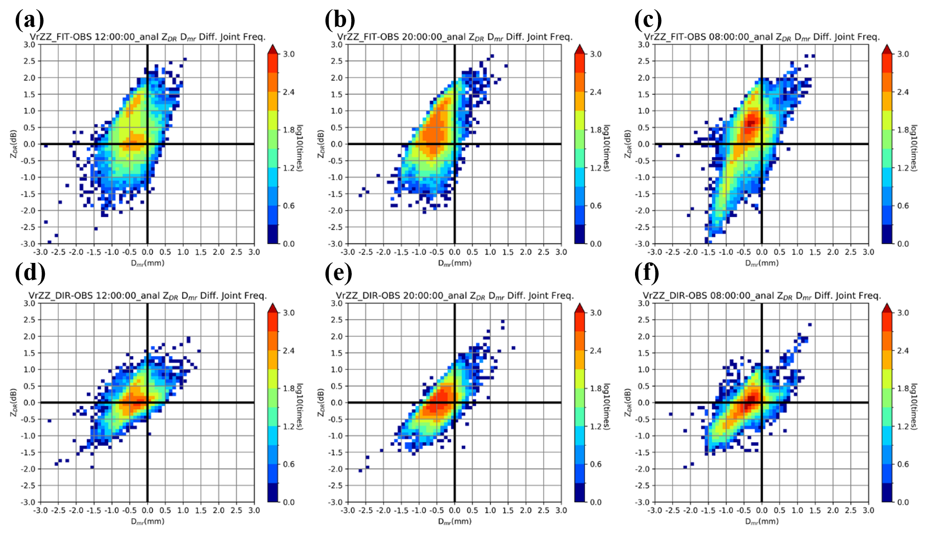
Figure 15 Analyzed D_mr–Z_DR joint frequency at the time of the final analyses in (a–c) VrZZ_FIT and (d–f) VrZZ_DIR experiments for the (a, d) squall line case, (b, e) typhoon case, and (c, f) Mei-Yu frontal case. The shading indicates the occurrence times on the logarithmic scale. The horizontal and vertical axes indicate D_mr and Z_DR with 0.1 mm and 0.1 dB intervals, respectively.

6 Conclusions

Cloud microphysics describes the interactions between hydrometeor species, which directly influence the growth and decay of rainfall systems and the intensity of precipitation. In monitoring the rapid development of rainfall systems, dual-polarization radar, in which electrometric waves in two directions are detected, can be used to obtain comprehensive insight into cloud microphysics and depict the bulk characteristic of the hydrometeor species. The characteristics of dual-polarization radar parameters have been widely used in particle identification, radar data QC and depicting the microphysical structure. Because the dual-polarization radar data are not prognostic variables in the numerical model, variable transformation is required before model validation and data assimilation can be performed. The observation operator can derive the observed variable in the observation space by using the predicted variable in the model space, leading to a more direct connection between the model and observation. Dual-polarization radar operators have been developed and utilized for data assimilation in several studies. Such operators have two major types of configuration: those using the fitting method and those using the direct integration method. Both methods calculate dual-polarization parameters by integrating scattering amplitudes over the given DSD. In the power-law fitting method, the scattering amplitudes are fitted as a function of diameter, enabling an analytical solution to the integration and improving computational efficiency; while in the direct integration method, the numerical integration is used to calculate the dual-polarization radar parameters directly. Different simulations of dual-polarization radar parameters may directly change the structure of the background error covariance, creating various results after DA. Hence, to obtain the most reasonable and unbiased background structure, simulations of dual-polarization parameters involving different types of operators should be evaluated. In this study, a dual-polarization radar operator established on the basis of that reported by Jung et al. (2008a) is used to simulate and assimilate dual-polarization radar data into the model. Additionally, the raindrop-contributed terms are obtained using the fitting method (Jung et al., 2008a) and the direct integration method (Jung et al., 2010) to describe the effect of operator configuration on data assimilation. Finally, three types of summertime rainfall events, including the squall line case, the typhoon case, and the Mei-Yu frontal case (quasi-stationary front), are selected to comprehensively validate the simulation in the real case.

The evaluation reveals that both configurations can simulate a reflectivity structure similar to that in observations. However, the simulated Z_DR using the fitting method has an unreasonable negative value below the melting layer, which occurs because of the limitations of power-law fitting. Compared with that obtained using the fitting method, the Z_DR simulated using the direct integration method is similar to the observation data, leading to a structure more similar to that in the observation. The same results are obtained from the Z_HH–Z_DR joint frequency diagram. The fitting method leads to negative value and overestimation of Z_DR when the reflectivity is greater than 30 dBZ. Instead, when the direct integration method is used, the high-occurrence region is closer to the observations than with the fitting method. In this case, the Z_DR difference between simulations and observations is limited to within ±0.6 dB. However, the overestimation of Z_DR still persists when the reflectivity exceeds 30 dBZ, even with the direct integration method. In addition, it could not comprehensively describe the spread of the joint frequency distribution, which indicates the operator has an insufficient degree of freedom. The performance of raindrop prognostic variables is validated to describe how dual-polarization radar data assimilation affects the model. The results reveal that assimilating dual-polarization radar parameters into the model do not clearly improve the D_mr simulation. However, using the direct integration method rather than the fitting method leads to a more favorable result; the relationship between the D_mr and Z_DR occurrence frequency is more concentrated and closer to the observed relationship. Crucially, both the forward operator and the MP scheme cannot exactly simulate the details of complex mechanism underlying the mesoscale system, and it may directly impact the short forecasts during DA cycling, diluting the advantages of the DA. These problems should be further studied to enable modification of the system and establish a suitable DA strategy to enhance the predictability.

To sum up, although using the power-law function to fit the scattering amplitude efficiently calculates the dual-polarization radar parameters, it also leads to unreasonable negative value in Z_DR simulation. By contrast, using the direct integration method to calculate the raindrop-contributed reflectivity factor can result in a more reasonable Z_HH and Z_DR structure and an acceptable D_mr structure after DA. However, this study also reveals some problems that have to be further investigated. Because the characteristics of hydrometeor species may differ for various configurations inside schemes, the microphysics processes in the short forecasts must be confirmed, and the most suitable scheme for simulating different weather systems should be identified. In terms of the dual-polarization radar observation operator, simulation related to ice particles has considerable uncertainty because ice particles can have various shapes and densities, and exhibit various canting motions. Finally, since the Z_HH and Z_DR bias in the background during DA cycling directly limits the effect of DA, except for the forward operator, the microphysics processes in MP schemes should be validated and optimized using the real time observation to ensure that simulations could preserve the benefits of assimilation during short forecasting.

Next, dual-polarization parameter simulations with different microphysics schemes, particularly the new version of the multi-moment microphysics schemes, should be validated with different weather cases. Additionally, we attempt to validate the benefits of assimilating different-waveband, non-operational regional weather radar data, which are often used in bean-blockage regions. Regarding the forward operator, it is necessary to test the initial setting of the ice particle T-matrix simulations must be further tested to adjust the ice contribution term to the observation.