Estimation of vertical profiles of raindrop size distribution and cloud microphysical processes in stratiform rainfall using vertical-pointing X- and VHF-band radars

Simultaneous vertical pointing observations by X- and VHF-band radars were conducted in Japan, and these data were used to estimate vertical profiles of drop size distribution (DSD) parameters of raindrops, assuming a gamma distribution, for a stratiform rainfall event. We used X-band reflectivity, vertical Doppler velocity, and spectral width, combined with VHF-band vertical air motion data. The estimation considers non-Rayleigh scattering and the influence of vertical air motion, and accounts for the contamination of spectral broadening using a forward convolution technique. We demonstrated that for stratiform rainfall, broadening by wind shear may be neglected, even with a relatively coarse radar range resolution of 150 m. Cloud physical quantities (median volume diameter, liquid water content, normalised intercept parameter) retrieved from the estimated DSD parameters were compared with operational X-band polarimetric radar data and found to be highly accurate. We also point out the potential applicability of this method to satellite-borne radars. Among the estimated parameters, the shape and slope parameters generally increased with decreasing altitude. These changes are attributed to collision-coalescence and breakup based on variations in the cloud physical quantities, likely due to the humid environment. This study suggests that retrieving cloud physical quantities from DSD parameters estimated from vertical observations enables robust discussions on cloud physical processes.

1 Introduction

The drop size distribution (DSD) of raindrops is a crucial parameter that is often used to discuss cloud microphysical processes. As DSD is necessary for estimating rain rate and liquid water content (LWC [g m⁻³]; e.g., Fukao and Hamazu, 2014), accurate DSD estimation can lead to a better understanding of precipitation phenomena. For example, the estimation of the rain rate from radar parameters (e.g., radar reflectivity factor (Z^∗ [mm⁶ m⁻³])) is influenced by the variation of the DSD (e.g., Fukao and Hamazu, 2014), leading to potential errors. DSD is also used in numerical models, including cloud physics parameterisation (e.g., Lin et al., 1983; Murakami, 1990; Ferrier, 1994; Seiki and Nakajima, 2014), and is important for the accurate reproduction and understanding of precipitation. For these reasons, many studies on DSD have been conducted.

Ulbrich (1983) assumed a gamma distribution to represent the DSD, denoted as N(D) [mm⁻¹ m⁻³], which is expressed as follows:

$$\begin{array}{}\text{(1)}& N\left(D\right)=N_{\mathrm{0}}{D}^{\mathit{\mu }}\exp \left(-\mathrm{\Lambda }D\right),\end{array}$$

where D [mm] is the equivalent diameter, N₀ [mm${}^{-\mathrm{1}-\mathit{\mu }}$ m⁻³] is the intercept parameter, μ is the shape parameter, and Λ [mm⁻¹] is the slope parameter. Tokay and Short (1996) analysed maritime precipitation separately as stratiform and convective rains using ground-based disdrometer data and indicated that stratiform precipitation has more raindrops with larger particle sizes and a smaller number concentration of small particle sizes than convective precipitation at the same precipitation intensity. This means that, assuming a gamma distribution, the value of Λ for stratiform precipitation is smaller than that for convective precipitation. Using disdrometer and radar data, Bringi et al. (2003) showed that the location of clustering is different for stratiform and convective precipitation in the relationship between mass-weighted mean diameter (D_m [mm]) and the normalised intercept parameter (N_w [mm⁻¹ m⁻³]). Bringi et al. (2009) and Thompson et al. (2015) also indicated that a line to distinguish between stratiform and convective precipitation can be drawn in the D_m–N_w plane. Furthermore, Bringi et al. (2003) also noted that, for convective precipitation, the position of clustering in the D_m–N_w plane is different for maritime and continental precipitation, and that D_m is smaller and N_w larger in maritime precipitation than in continental precipitation. Dolan et al. (2018) conducted a principal component analysis using disdrometer observations for various latitude bands and precipitation types and showed that DSDs can be classified into six groups. However, Dolan et al. (2018) also showed that certain groups hardly appear in specific latitudinal zones and that the range of DSD parameters assuming a gamma distribution (N₀, μ, and Λ) varies across latitudinal zones. Thus, DSD varies depending on precipitation type, latitudinal zone, and geography, such as oceanic or continental regions. Recently, studies on DSD using disdrometers have also been increasing in East Asia. For example, Suh et al. (2021) conducted disdrometer observations at multiple sites in South Korea and showed that D_m increases while N_w decreases as the distance from the coast increases, even during stratiform precipitation. Seela et al. (2018) examined the DSD of summer and winter rainfall in Taiwan and found that summer rainfall had larger raindrops than winter rainfall. They attributed this to larger ice crystals falling from the upper levels due to the greater convective available potential energy and amount of water vapour in summer. Tsuji et al. (2024) studied oceanic rainfall in Japan using disdrometer data for two years and classified it into two groups with the same precipitation intensity: one with larger raindrop sizes and the other with higher number concentrations. They concluded that the former is characterised by ice-phase processes in deep clouds and the latter by warm rain processes in shallow clouds, based on brightness temperatures observed by satellites. These studies primarily extract parameters related to DSD from ground-based observations and combine them with other data to estimate cloud microphysical processes; however, they do not provide detailed insight into the vertical changes in DSD parameters aloft. As DSD parameters on the ground are the result of various cloud microphysical processes aloft, the simultaneous estimation of cloud microphysical processes and vertical variations in DSD parameters is essential for clarifying the mechanisms of precipitation formation. Therefore, obtaining accurate vertical profiles of DSD parameters is crucial.

To address this need, several methods using radar for estimating the vertical profile of DSD parameters have been proposed. Fukao and Hamazu (2014) showed that, assuming a gamma distribution, the DSD can be estimated from Z^∗, mean vertical Doppler velocity ($\stackrel{\mathrm{‾}}{V_{\mathrm{d}}}$ [m s⁻¹]), and Doppler velocity spectrum width (σ_d [m s⁻¹]) obtained from a single vertical pointing radar if the Rayleigh scattering approximation is valid and mean vertical air motion (${\stackrel{\mathrm{‾}}{V}}_{\mathrm{a}}$ [m s⁻¹]) can be ignored. Methods for accounting for the effect of vertical air motion have also been explored, with several studies highlighting the importance of separating DSD and ${\stackrel{\mathrm{‾}}{V}}_{\mathrm{a}}$. VHF- or UHF-band radars are often used to estimate the vertical profile of DSD parameters because the sensitivity of these radars is influenced by both Bragg scattering from turbulence in clear air and Rayleigh scattering from precipitation particles (e.g., Wakasugi et al., 1986; Gossard, 1988). However, as the radar cross-section of Rayleigh scattering is inversely proportional to the fourth power of the wavelength (e.g., Gossard, 1988), the VHF-band radar cannot detect weak rain (Rajopadhyaya et al., 1993). Similarly, the UHF-band radar also has the disadvantage that Bragg scattering is significantly overwhelmed by Rayleigh scattering in moderate to heavy rain (Rajopadhyaya et al., 1998). Therefore, instead of a single profiler method, a dual-frequency method has been proposed that combines VHF- and UHF-band radars to easily separate the echoes caused by precipitation particles from clear-air turbulence echoes (e.g., Rajopadhyaya et al., 1998; Rao et al., 2006; Kirankumar et al., 2008). In this method, the spectra obtained from VHF-band radar clearly reflect the influence of clear-air turbulence, and thus these spectra are applied to the UHF spectra to estimate the rain rate and the median volume diameter (D₀ [mm]). Rajopadhyaya et al. (1998) reported that it is important to correct for the contamination of $\stackrel{\mathrm{‾}}{V_{\mathrm{d}}}$ caused by ${\stackrel{\mathrm{‾}}{V}}_{\mathrm{a}}$ and that of σ_d caused by spectral broadening when estimating the rain rate and D₀, especially because the uncorrected $\stackrel{\mathrm{‾}}{V_{\mathrm{d}}}$ can be a significant source of error. The dual-frequency method has also been employed in combinations of other higher-frequency bands. Pang et al. (2021) combined L- and C-band vertical pointing radars, used inverse convolution to remove contamination due to turbulence, and then estimated DSD. Matrosov (2017) indicated the relationship between D_m and Doppler velocity difference using Ka- and W-band vertical pointing radars. Williams et al. (2016) calculated the Doppler velocity difference using S- and Ka-band vertical pointing radars and combined these results with the Z^∗ and σ_d to estimate the three parameters of the gamma distribution and ${\stackrel{\mathrm{‾}}{V}}_{\mathrm{a}}$. As shown above, various frequency bands are used to obtain DSD through vertical observations. Higher-frequency radars have the benefit of being more sensitive to precipitation particles, while the Rayleigh scattering approximation becomes invalid for large raindrops (e.g., Ryzhkov and Zrnic, 2019) and the data processing becomes complex.

Considering both altitude changes in DSD and cloud microphysical processes simultaneously should be useful for improving cloud physics parameterisations, as altitude variations in DSD are the result of cloud microphysical processes. Some previous studies have suggested that the predominant cloud microphysical processes of raindrops, such as collision-coalescence, collision-breakup, and evaporation, can be inferred from altitude variations in the DSD parameters. For example, Rao et al. (2006) and Kirankumar et al. (2008) estimated that evaporation is predominant because μ and/or Λ increase with decreasing altitude in the tropics. Meanwhile, Barthes and Mallet (2013) conducted numerical experiments on a one-dimensional rain shaft, taking coalescence and breakup into account, and demonstrated that μ increases as raindrops fall. Williams et al. (2016) inferred that coalescence is predominant based on a single profile in which D_m increases downward. However, Xie et al. (2016) conducted numerical experiments considering evaporation and demonstrated that D₀ can also increase due to evaporation, except for specific DSDs (e.g., initial μ<2 and D₀>2.3 mm with 5 mm h⁻¹). Thus, even if the altitude variation of the DSD parameters is the same, the predominant cloud microphysical processes may differ. Such uncertainties in estimating cloud microphysical processes from vertical pointing observations should be avoided by considering the vertical variation of multiple cloud physical quantities (e.g., D₀, LWC, and N_w), which are estimated from retrieved DSD parameters.

Simultaneous vertical observations by X- and VHF-band radars have been conducted in Japan since January 2023. In this study, we propose methods to investigate the detailed vertical variation of DSD parameters assuming a gamma distribution using X- and VHF-band radar data and to estimate the predominant microphysical processes using multiple cloud physical quantities derived from these estimated DSD parameters. This combination is advantageous for extracting the vertical profiles of DSD parameters because the frequencies are widely separated; they are highly sensitive to rain and vertical air motion, respectively. X-band radars have higher frequencies than C- and S-band radars, which results in larger backscattering cross sections under the Rayleigh scattering approximation (e.g., Fukao and Hamazu, 2014) and offers the benefit of higher sensitivity to smaller raindrops. In addition, our method has the advantage of reducing ${\stackrel{\mathrm{‾}}{V}}_{\mathrm{a}}$ uncertainties by using directly retrieved ${\stackrel{\mathrm{‾}}{V}}_{\mathrm{a}}$ data from VHF-band radar rather than indirect estimates. We discuss the influence of contamination caused by ${\stackrel{\mathrm{‾}}{V}}_{\mathrm{a}}$, horizontal wind speed, and turbulence on DSD parameter estimation. We consider the non-Rayleigh effect by performing scattering simulations. We also compare the retrieved cloud physical quantities with data from an operational X-band dual-polarimetric radar that performs plan position indicator (PPI) observations and confirm the validity of vertical pointing observations in X- and VHF-band radars. Furthermore, while the next-generation satellite-borne precipitation radar of the Precipitation Measuring Mission (PMM) is a Ku-band Doppler radar (Nakamura and Furukawa, 2023; Kanemaru et al., 2024), we discuss how accurately DSD can be estimated by using X-band Doppler radars operating at frequencies close to that of Ku-band (e.g., Goto et al., 2025). To rigorously evaluate the accuracy of this estimation method, this study targets stratiform rainfall, which is expected to be less influenced by vertical air motion and non-uniform beam filling than convective rainfall (e.g., Durden et al., 1998). In Sect. 2, the radars used in this study are introduced. Section 3 presents the methods of data processing. Section 4 provides an overview of the analysis of a stratiform rainfall case, confirms the accuracy of the DSD estimated from vertical pointing observations by X- and VHF-band radars, and estimates and discusses the cloud microphysical processes that contribute to the change in altitude of the DSD parameters. Section 5 is the summary.

2 Instruments

2.1 Middle and upper atmosphere (MU) radar

The middle and upper atmosphere (MU) radar in Japan is a Doppler radar with a phased array system, consisting of 475 crossed Yagi antennas, and operates at a frequency of 46.5 MHz, i.e., a VHF-band radar (Fukao et al., 1985, 1990). The MU radar is located at the Shigaraki MU Observatory and is 372 m above the mean sea level (a.m.s.l.). The specifications of the MU radar are listed in Table 1 and the location is shown in Fig. 1. In this study, only vertical pointing data in tropospheric observation mode, which is characterised by a high range resolution (150 m), were used to remove the effect of ${\stackrel{\mathrm{‾}}{V}}_{\mathrm{a}}$. As the analysis is limited to the liquid phase, only data at altitudes of about 3400 m or less were used. The mean vertical air motion, as a 1 min value derived by the MU radar ($\stackrel{\mathrm{‾}}{V_{\mathrm{a}}^{\mathrm{MU}}}$ [m s⁻¹]), was used to remove the effects of ${\stackrel{\mathrm{‾}}{V}}_{\mathrm{a}}$ from the vertical Doppler velocity of the X-band radar (NUX, as described in Sect. 2.2). Notably, $\stackrel{\mathrm{‾}}{V_{\mathrm{a}}^{\mathrm{MU}}}$ is equivalent to ${\stackrel{\mathrm{‾}}{V}}_{\mathrm{a}}$ in this study. The spectral width of vertical air motion (σ_a [m s⁻¹]) derived by the MU radar (${\mathit{\sigma }}_{\mathrm{a}}^{\mathrm{MU}}$ [m s⁻¹]) was also used to restrict the time of the analysis (as described in Sect. 3.2).

Table 1 Specifications of the MU radar in tropospheric observation mode (Fukao et al., 1990; Fukao and Hamazu, 2014).

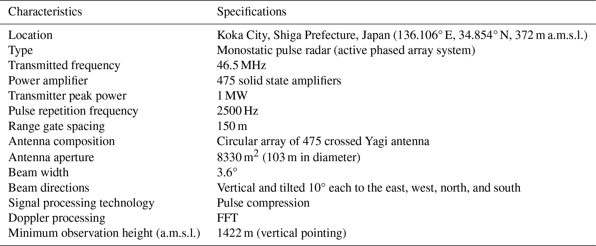
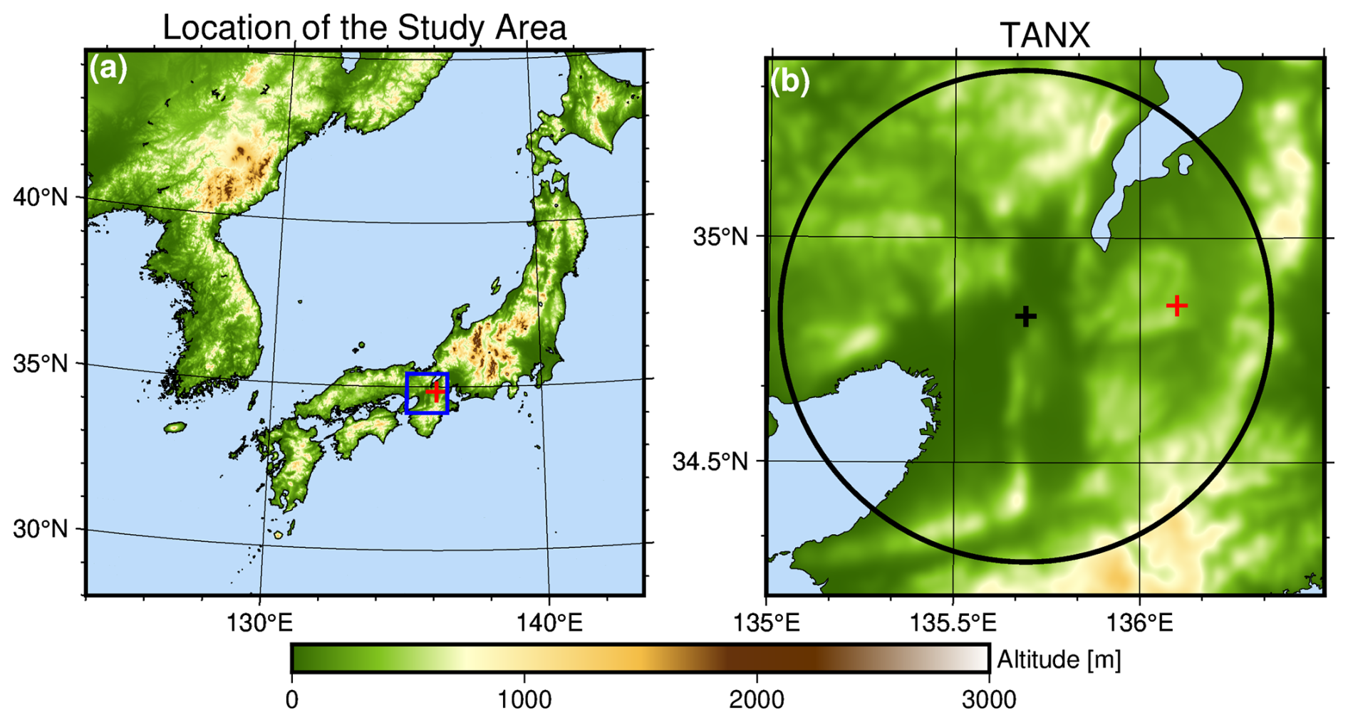
Figure 1 (a) The location of the study area. The blue rectangle shows the areas in (b). The red + marks in (a) and (b) indicate the location of the Shigaraki MU Observatory. The black + mark and circle in (b) indicate the location of the operational X-band polarimetric radar (Tanokuchi radar; TANX) that was used for validation and its observation range (radius of 60 km), respectively.

2.2 X-band radar of Nagoya University (NUX)

The X-band radar of Nagoya University (Morotomi et al., 2012; hereafter NUX) is a mobile polarimetric Doppler radar. The specifications are presented in Table 2. The NUX has been installed within the Shigaraki MU Observatory (Fig. 1) since January 2023 and conducts vertical pointing observations for 4 min of every 5 min. During vertical observations, the NUX rotates 360° in azimuth every 30 s. The radar reflectivity factor (Z^∗NUX [mm⁶ m⁻³]), mean vertical Doppler velocity of the spectrum ($\stackrel{\mathrm{‾}}{{V_{\mathrm{d}}}^{\mathrm{NUX}}}$ [m s⁻¹]), and Doppler velocity spectral width (${\mathit{\sigma }}_{\mathrm{d}}^{\mathrm{NUX}}$ [m s⁻¹]) obtained from the NUX were used to estimate the vertical profile of DSD parameters assuming a gamma distribution. As NUX does not output raw spectral information, the Doppler velocity spectral width, processed internally and output by the radar, was used in this study. The Z^∗ is often expressed as the radar reflectivity ($Z=\mathrm{10}{\log }_{\mathrm{10}}{Z}^{\ast }$ [dBZ]), and the Z obtained from the NUX (Z^NUX [dBZ]) was also used.

Table 2 Specifications of the NUX during vertical observation and at an elevation angle of 20°.

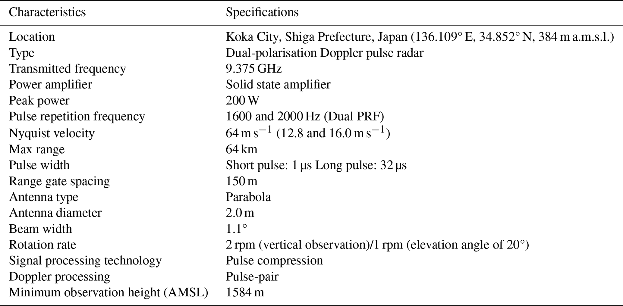
We also used $\stackrel{\mathrm{‾}}{{V_{\mathrm{d}}}^{\mathrm{NUX}}}$ data at an elevation angle of 20° for the calibration of ${\mathit{\sigma }}_{\mathrm{d}}^{\mathrm{NUX}}$. Observations at an elevation angle of 20° were conducted once every five minutes.

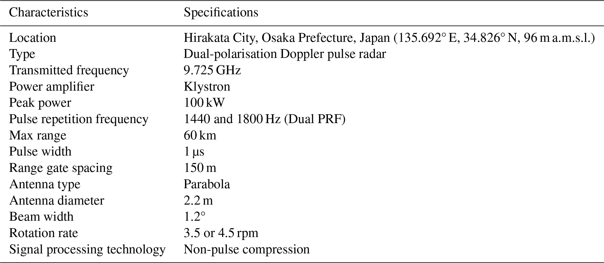
2.3 Operational X-band polarimetric radar (TANX)

For comparison of estimated cloud physical quantities and dominant cloud microphysics, data from an operational X-band polarimetric Doppler radar located about 38 km away from the Shigaraki MU Observatory were also used (Fig. 1b). This X-band radar is one of the radars in the eXtended RAdar Information Network (XRAIN) operated by the Ministry of Land, Infrastructure, Transport and Tourism in Japan, and this study utilises the radar at Tanokuchi station (TANX). The specifications are presented in Table 3. The TANX performs one volume scan at 12 elevation angles every 5 min, while conducting multiple low-elevation scans, resulting in a total of 15 PPI scans every 5 min. The elevations of the TANX are set between 0.9 and 15.0°. The variables used from the TANX were the horizontal radar reflectivity factor (Z^∗TANX [mm⁶ m⁻³]), horizontal radar reflectivity (Z^TANX [dBZ]), differential reflectivity ($Z_{\mathrm{DR}}^{\mathrm{TANX}}$ [dB]), and specific differential phase ($K_{\mathrm{DP}}^{\mathrm{TANX}}$ [degree km⁻¹]).

Table 3 Specifications of the TANX.

3 Data processing

3.1 NUX variables used for estimating DSD parameters

The reflectivity factor (Z^∗), mean vertical Doppler velocity ($\stackrel{\mathrm{‾}}{V_{\mathrm{d}}}$), and Doppler velocity spectral width (σ_d) assuming Rayleigh scattering approximation, obtained from the vertical pointing radar observations, are expressed by the following equations, respectively (Fukao and Hamazu, 2014):

$$\begin{array}{}\text{(2)}& {\displaystyle }{Z}^{\ast }={\int }_{D_{\min }}^{D_{\max }}{D}^{\mathrm{6}}N\left(D\right)\mathrm{d}D,\text{(3)}& {\displaystyle }\stackrel{\mathrm{‾}}{V_{\mathrm{d}}}=-{\displaystyle \frac{{\int }_{D_{\min }}^{D_{\max }}{V}_t\left(D\right)D^{\mathrm{6}}N\left(D\right)\mathrm{d}D}{{\int }_{D_{\min }}^{D_{\max }}{D}^{\mathrm{6}}N\left(D\right)\mathrm{d}D}}+{\stackrel{\mathrm{‾}}{V}}_{\mathrm{a}},\text{(4)}& {\displaystyle }{\mathit{\sigma }}_{\mathrm{d}}=\sqrt{{\displaystyle \frac{{\int }_{D_{\min }}^{D_{\max }}{\left\{V_t\left(D\right)\right\}}^{\mathrm{2}}{D}^{\mathrm{6}}N\left(D\right)\mathrm{d}D}{{\int }_{D_{\min }}^{D_{\max }}{D}^{\mathrm{6}}N\left(D\right)\mathrm{d}D}}-{\left({\displaystyle \frac{{\int }_{D_{\min }}^{D_{\max }}{V}_t\left(D\right)D^{\mathrm{6}}N\left(D\right)\mathrm{d}D}{{\int }_{D_{\min }}^{D_{\max }}{D}^{\mathrm{6}}N\left(D\right)\mathrm{d}D}}\right)}^{\mathrm{2}}},\end{array}$$

where V_t(D) [m s⁻¹] is the fall velocity of the precipitation particles, and D_max and D_min [mm] are the maximum and minimum sizes of the precipitation particles, respectively. Note that N(D) is assumed to be a gamma distribution function as in Eq. (1). As this study deals with raindrops, V_t(D) was used with the following equation (Atlas et al., 1973; Fukao and Hamazu, 2014),

$$\begin{array}{}\text{(5)}& V_t\left(D\right)=\left(\mathrm{9.65}-\mathrm{10.3}{e}^{-\mathrm{0.6}D}\right){\left({\displaystyle \frac{{\mathit{\rho }}_{\mathrm{a}\mathrm{0}}}{{\mathit{\rho }}_{\mathrm{a}}}}\right)}^{\mathrm{0.4}},\end{array}$$

where ρ_a0 and ρ_a [kg m⁻³] are the air density of the International Standard Atmosphere (=1.225 kg m⁻³) and the ambient air, respectively. ρ_a is calculated by linear interpolation of pressure and temperature data from ERA5 (Hersbach et al., 2020) to the observed grid points and using the equation of state for a dry atmosphere. As ERA5 collects hourly data, the data from ERA5 closest to the vertical observation time is used. For Eqs. (3) and (5), the fall velocity of a raindrop is generally expressed as a positive value, while the Doppler velocity and vertical air motion are expressed as a positive value in the direction away from the ground-based radar. To adjust the sign, the first term on the right side of Eq. (3) is multiplied by −1.

Equations (2)–(4) assume that the Rayleigh scattering approximation holds; however, the X-band radar (NUX) could produce errors resulting from the limitations of the Rayleigh scattering approximation. Figure 2 shows the relationship between raindrop diameter and backscattering cross section of the NUX, calculated by scattering simulations using the T-matrix method (Waterman, 1971) with the PyTmatrix package (Leinonen, 2014), for raindrop diameters up to a maximum of 9 mm (Pruppacher and Klett, 1997). The figure indicates that when the diameter exceeds about 2.5 mm, the resonance in the induced electric field becomes significant and the Rayleigh scattering approximation is no longer valid. Therefore, in this study, non-Rayleigh scattering was also considered following Williams et al. (2016), and is expressed as follows:

$$\begin{array}{}\text{(6)}& {\displaystyle }{Z}^{\ast \mathrm{nonRay}}={\displaystyle \frac{{\mathit{\lambda }}^{\mathrm{4}}}{{\mathit{\pi }}^{\mathrm{5}}{\left|K\right|}^{\mathrm{2}}}}{\int }_{D_{\min }}^{D_{\max }}{\mathit{\sigma }}_{\mathrm{b}}\left(D\right)N\left(D\right)\mathrm{d}D,\text{(7)}& {\displaystyle }\stackrel{\mathrm{‾}}{V_{\mathrm{d}}^{\mathrm{nonRay}}}=-{\displaystyle \frac{{\int }_{D_{\min }}^{D_{\max }}{V}_t\left(D\right){\mathit{\sigma }}_{\mathrm{b}}\left(D\right)N\left(D\right)\mathrm{d}D}{{\int }_{D_{\min }}^{D_{\max }}{\mathit{\sigma }}_{\mathrm{b}}\left(D\right)N\left(D\right)\mathrm{d}D}}+{\stackrel{\mathrm{‾}}{V}}_{\mathrm{a}},\text{(8)}& {\displaystyle }\begin{array}{rl}{\mathit{\sigma }}_{\mathrm{d}}^{\mathrm{nonRay}}& =\sqrt{{\displaystyle \frac{{\int }_{D_{\min }}^{D_{\max }}{\left\{V_t\left(D\right)\right\}}^{\mathrm{2}}{\mathit{\sigma }}_{\mathrm{b}}\left(D\right)N\left(D\right)\mathrm{d}D}{{\int }_{D_{\min }}^{D_{\max }}{\mathit{\sigma }}_{\mathrm{b}}\left(D\right)N\left(D\right)\mathrm{d}D}}}\\ & \stackrel{\mathrm{‾}}{-{\left({\displaystyle \frac{{\int }_{D_{\min }}^{D_{\max }}{V}_t\left(D\right){\mathit{\sigma }}_{\mathrm{b}}\left(D\right)N\left(D\right)\mathrm{d}D}{{\int }_{D_{\min }}^{D_{\max }}{\mathit{\sigma }}_{\mathrm{b}}\left(D\right)N\left(D\right)\mathrm{d}D}}\right)}^{\mathrm{2}}},\end{array}\end{array}$$

where λ [mm] is the wavelength of the radar, |K|² is the dielectric factor with a value of 0.93 for raindrops and X-band radars (Gunn and East, 1954), and σ_b [mm²] is the backscattering cross section. The first term on the right side of Eq. (7) is equivalent to $\stackrel{\mathrm{‾}}{V_{tz}^{\mathrm{nonRay}}}$ [m s⁻¹].

Figure 2 (a) Relationship between the size of a sphere and the backscattering cross section, and (b) an enlarged view. The blue line is obtained from a scattering simulation using the T-matrix method, and the orange line assumes Rayleigh scattering. For this simulation, the wavelength is 32 mm (X-band), the raindrop temperature is 10 °C, and the raindrop shape is assumed to be a sphere.

3.2 Reducing the influence of ${\mathit{\sigma }}_{\mathrm{d}}^{\mathrm{NUX}}$ broadening

The σ_d from vertical pointing observations is mainly due to the size spread of precipitation particles (σ_DSD); however, the spread is also influenced by horizontal wind, turbulence, and wind shear (e.g., Shupe et al., 2008; Williams et al., 2016). Therefore, ${\mathit{\sigma }}_{\mathrm{d}}^{\mathrm{NUX}}$ is slightly larger owing to various contaminations, although the estimation of DSD should only consider the σ_DSD. This broadening is expressed as the sum of the variances, as follows (Shupe et al., 2008; Williams et al., 2016):

$$\begin{array}{}\text{(9)}& {\mathit{\sigma }}_{\mathrm{broadening}}^{\mathrm{2}}={\mathit{\sigma }}_{\mathrm{H}}^{\mathrm{2}}+{\mathit{\sigma }}_{\mathrm{T}}^{\mathrm{2}}+{\mathit{\sigma }}_{\mathrm{S}}^{\mathrm{2}},\end{array}$$

where ${\mathit{\sigma }}_{\mathrm{H}}^{\mathrm{2}}$, ${\mathit{\sigma }}_{\mathrm{T}}^{\mathrm{2}}$, and ${\mathit{\sigma }}_{\mathrm{S}}^{\mathrm{2}}$ are terms attributed to horizontal wind speed, turbulence, and wind shear, respectively. Williams et al. (2016) pointed out that ${\mathit{\sigma }}_{\mathrm{H}}^{\mathrm{2}}$ and ${\mathit{\sigma }}_{\mathrm{T}}^{\mathrm{2}}$ are particularly significant and also noted that corrections should be applied for radar beamwidths of 3° or greater. Rajopadhyaya et al. (1998) indicated that the estimated D_m would have an error of about 15 % if no correction was made for the σ_d broadening of the UHF-band radar. Notably, the UHF-band radar beamwidth used in Rajopadhyaya et al. (1998) is 9° . The beam width of the NUX used in this study is 1.1° (Table 2) and the contamination due to broadening is expected to be small; however, efforts should be made to minimise errors because the influence of broadening varies depending on the surrounding atmospheric conditions, even when the beamwidth is relatively small. Gossard and Strauch (1983) expressed the broadening variance due to horizontal wind (${\mathit{\sigma }}_{\mathrm{H}}^{\mathrm{2}}$) using the following equation:

$$\begin{array}{}\text{(10)}& {\mathit{\sigma }}_{\mathrm{H}}^{\mathrm{2}}={\displaystyle \frac{U^{\mathrm{2}}{\mathit{\phi }}^{\mathrm{2}}}{\mathrm{2.76}}},\end{array}$$

where U [m s⁻¹] is horizontal wind speed and φ [radian] is radar beam width. Furthermore, assuming an inertial sub-range, the contribution of turbulence is given by the following equation (Shupe et al., 2008):

$$\begin{array}{}\text{(11)}& {\displaystyle \frac{{\mathit{\sigma }}_{\mathrm{T}}^{\mathrm{2}}}{{\mathit{\sigma }}_{\mathrm{measurement}}^{\mathrm{2}}}}\approx {\displaystyle \frac{L_{\mathrm{s}}^{\mathrm{2}/\mathrm{3}}}{L_{\mathrm{l}}^{\mathrm{2}/\mathrm{3}}-L_{\mathrm{s}}^{\mathrm{2}/\mathrm{3}}}},\end{array}$$

where ${\mathit{\sigma }}_{\mathrm{measurement}}^{\mathrm{2}}$ is the Doppler velocity width obtained from observations, and in this study, it is the square of the Doppler velocity spectral width (${\mathit{\sigma }}_{\mathrm{d}}^{\mathrm{NUX}}$) averaged over 30 s interval. In this study, L_s is the length of the scattering volume for 0.1 s dwell time and L_l indicates the larger eddies passing through the effective sample volume that results from an average of the radar observations over 30 s. L is expressed by the following equation (Shupe et al., 2008):

$$\begin{array}{}\text{(12)}& L=Ut+\mathrm{2}R\sin \left({\displaystyle \frac{\mathit{\phi }}{\mathrm{2}}}\right),\end{array}$$

where t [s] is time and R [m] is the distance from the radar to the observation grid point. Equations (10) and (12) show that the horizontal wind aloft is important in addition to the radar beam width. Additionally, the effect of horizontal and vertical shear in the vertical winds is expressed by the following equation (Gossard and Strauch, 1983; Shupe et al., 2008):

$$\begin{array}{}\text{(13)}& {\mathit{\sigma }}_{\mathrm{S}}^{\mathrm{2}}={\displaystyle \frac{k_{\mathrm{h}}^{\mathrm{2}}{R}^{\mathrm{2}}{\mathit{\phi }}^{\mathrm{2}}}{\mathrm{2.76}}}+{\displaystyle \frac{k_{\mathrm{v}}^{\mathrm{2}}{\mathrm{\Delta }}^{\mathrm{2}}}{\mathrm{12}}},\end{array}$$

where k_h and k_v [s⁻¹] are the horizontal shear in vertical wind and vertical shear in vertical wind, respectively. Δ [m] is the range gate spacing. Note that while the effects of wind shear are often neglected in previous studies (e.g., Williams et al., 2016; Pang et al., 2021), the range resolution of the NUX used in this study is 150 m (Table 2), which is about 2 to 5 times coarser than that of previous studies. Therefore, the potential influence of broadening due to shear is examined in this study. In addition, to minimize contamination caused by vertical air motion and spectral broadening, the method for estimating the vertical profile of DSD parameters in this study was applied only to typical stratiform rainfall, which is expected to have small temporal and vertical variations in wind. Rao et al. (1999) gave an example of the vertical structure of ${\stackrel{\mathrm{‾}}{V}}_{\mathrm{a}}$ and σ_a in stratiform and convective clouds based on VHF-band radar data, showing that the absolute value of ${\stackrel{\mathrm{‾}}{V}}_{\mathrm{a}}$ and the value of σ_a are both smaller in stratiform clouds than in convective clouds. Based on the data presented by Rao et al. (1999), typical stratiform rainfall is defined as rainfall that satisfies the following conditions: (I) $\left|\stackrel{\mathrm{‾}}{V_{\mathrm{a}}^{\mathrm{MU}}}\right|\le \mathrm{1.0}$ m s⁻¹ at all altitudes in the liquid phase, and (II) a mean of ${\mathit{\sigma }}_{\mathrm{a}}^{\mathrm{MU}}$, denoted as ($\stackrel{\mathrm{‾}}{{\mathit{\sigma }}_{\mathrm{a}}^{\mathrm{MU}}}$), is ≤1.2 m s⁻¹ in the liquid phase. Notably, the beamwidth of the VHF-band radar used by Rao et al. (1999) was 3.0°, and that of the MU radar is 3.6° (Table 1); thus, small differences in σ_a due to beamwidth are expected. The 0 °C altitude was identified using ERA5, the thickness of the melting layer was set as 1500 m following Rosenfeld et al. (1995), and the zone below the melting layer was defined as the liquid phase.

To consider the influence of ${\mathit{\sigma }}_{\mathrm{d}}^{\mathrm{NUX}}$ broadening, the wind speed aloft must be estimated. We applied the Velocity Azimuth Display (VAD) method (Browning and Wexler, 1968) using Doppler velocity data from NUX ($\stackrel{\mathrm{‾}}{{V_{\mathrm{d}}}^{\mathrm{NUX}}}$) at an elevation angle of 20° to estimate the wind speed aloft. In this study, calculations were performed using the linear least squares method (Tsuboki and Wakahama, 1988). Figure 3 shows a typical example of the horizontal wind speed aloft estimated using the VAD method based on the Doppler velocity from NUX. Throughout the analysis period, a west-southwesterly wind (as shown in Fig. 3b) prevailed for much of the time, with speeds of 10 to 30 m s⁻¹ (as shown in Fig. 3a). For such wind fields, ${\mathit{\sigma }}_{\mathrm{H}}^{\mathrm{2}}$ (Eq. 10) is on the order of 10⁻² to 10⁻¹. Additionally, we have confirmed that the ${\mathit{\sigma }}_{\mathrm{measurement}}^{\mathrm{2}}$ of NUX is around 0.03 m² s⁻² (not shown), and that ${\mathit{\sigma }}_{\mathrm{T}}^{\mathrm{2}}$ (Eq. 11) ranges from 10⁻³ to 10⁻² in magnitude. This implies that ${\mathit{\sigma }}_{\mathrm{H}}^{\mathrm{2}}$ and ${\mathit{\sigma }}_{\mathrm{T}}^{\mathrm{2}}$ may affect the estimation of DSD parameters; therefore, this study corrects for the broadening caused by these factors.

Figure 3 (a) Horizontal wind speed estimated using the VAD method and (b) horizontal distribution of NUX Doppler velocity at 15:39 JST (UTC + 9 h) on 2 June 2023. In (b), NUX is at the centre; warm colours indicate Doppler velocity away from the radar, and cool colours indicate Doppler velocity toward the radar. The grey circles in (b) indicate, from the innermost to the outermost, locations at 1500, 2000, 2500, 3000, and 3500 m altitude.

In addition, regarding corrections for shear, we focus on the vertical shear of vertical winds. Figure 4 shows the vertical change in vertical air motion derived from the $\stackrel{\mathrm{‾}}{V_{\mathrm{a}}^{\mathrm{MU}}}$, and even at the 99th percentile, k_v is calculated to be 0.0023 s⁻¹. Even when this 99th percentile value is substituted into the second term on the right-hand side of Eq. (13), the estimated variance remains on the order of 10⁻³ m² s⁻², even with Δ=150 m. This indicates that the effect of ${\mathit{\sigma }}_{\mathrm{S}}^{\mathrm{2}}$ is negligible because the values are less than 0.01 m² s⁻² in most cases (e.g., Pang et al., 2021), during the defined period of typical stratiform rainfall, even for radars with a relatively coarse range gate length (∼150 m). Note that the beam width at a distance of 3000 m from NUX is approximately 60 m, which is less than half the range gate length. Therefore, the broadening effect due to horizontal shear in vertical air motions is expected to be smaller than that due to vertical shear in vertical air motions, and can thus be neglected.

Figure 4 Histogram of vertical changes in vertical air motion during typical stratiform rainfall, determined from MU radar data. N is the total number of this samples.

3.3 Forward calculation of the Doppler spectrum via convolution of DSD effects and broadening

To remove the influence of σ_d broadening, several previous studies (e.g., Shupe et al., 2008; Williams et al., 2016) have assumed the following equation and removed the broadening effect through simple subtraction from ${\mathit{\sigma }}_{\mathrm{d}}^{\mathrm{2}}$:

$$\begin{array}{}\text{(14)}& {\mathit{\sigma }}_{\mathrm{d}}^{\mathrm{2}}\approx {\mathit{\sigma }}_{\mathrm{DSD}}^{\mathrm{2}}+{\mathit{\sigma }}_{\mathrm{broadening}}^{\mathrm{2}}.\end{array}$$

However, this assumption applies only when the radar reflectivity-weighted Doppler spectral density at each Doppler velocity (v) [m s⁻¹] generated by DSD in still air (S_DSD(v)) [(mm⁶ m⁻³)(m s${}^{-\mathrm{1}}{)}^{-\mathrm{1}}$] can be assumed to be Gaussian (Williams et al., 2016). As the Doppler spectrum generated by DSD does not necessarily follow a Gaussian distribution (e.g., black line in Fig. 5a), the convolution calculation should be considered rigorously. Therefore, we use the following convolution calculations (e.g., Zhu et al., 2023) for a rigorous estimation of the DSD parameters:

$$\begin{array}{}\text{(15)}& S_{\mathrm{Doppler}}\left(v\right)=S_{\mathrm{DSD}}\left(v\right)\otimes S_{\mathrm{broadening}}\left(v\right),\end{array}$$

where S_Doppler(v) [(mm⁶ m⁻³)(m s${}^{-\mathrm{1}}{)}^{-\mathrm{1}}$] is the radar reflectivity-weighted Doppler velocity spectral density and S_broadening(v) [(m s${}^{-\mathrm{1}}{)}^{-\mathrm{1}}$] is the spectral broadening due to the horizontal wind speed and turbulence. The ⊗ symbol represents convolution. Note that S_DSD(v) and S_broadening(v) are expressed by the following equations, respectively (Zhu et al., 2023):

$$\begin{array}{}\text{(16)}& {\displaystyle }{S}_{\mathrm{DSD}}\left(v\right)=N\left(D\right){\mathit{\sigma }}_{\mathrm{b}}\left(D\right){\displaystyle \frac{\mathrm{d}D}{\mathrm{d}{V}_t}},\text{(17)}& {\displaystyle }{S}_{\mathrm{broadening}}\left(v\right)={\displaystyle \frac{\mathrm{1}}{{\mathit{\sigma }}_{\mathrm{broadening}}\sqrt{\mathrm{2}\mathit{\pi }}}}\times \exp \left\{-{\displaystyle \frac{\mathrm{1}}{\mathrm{2}}}{\left({\displaystyle \frac{v}{{\mathit{\sigma }}_{\mathrm{broadening}}}}\right)}^{\mathrm{2}}\right\}.\end{array}$$

Figure 5 shows examples of the shape variations in the normalised Doppler spectral density when varying the values of μ and Λ at D₀=1.1 mm. When $\mathit{\mu }=-\mathrm{1}$ (Fig. 5a), the shape is less smooth than that in Fig. 5b due to the influence of non-Rayleigh scattering. The influence of broadening is reflected through the convolution calculation. The observed ${\mathit{\sigma }}_{\mathrm{d}}^{\mathrm{NUX}}$ corresponds to the theoretical standard deviation calculated after accounting for the broadening shown in Fig. 5.

Figure 5 Normalised Doppler spectral density calculated for a gamma DSD with D₀=1.1 mm, when (a) $\mathit{\mu }=-\mathrm{1}$ and (b) μ=1 are applied. The wavelength is assumed to be the same as that of NUX (=32 mm), and the effects of non-Rayleigh scattering are also considered using results from scattering simulations performed with the T-matrix method. The black line represents still air conditions, while the blue and red lines indicate broadening variance of 0.05 and 0.10 m² s⁻², respectively. The Std Dev in the figure represents the standard deviation of the spectrum, with the colour corresponding to the ${\mathit{\sigma }}_{\mathrm{broadening}}^{\mathrm{2}}$ magnitudes or still air.

3.4 Methods for estimating the vertical profile of DSD parameters

To account for non-Rayleigh scattering and estimate the DSD parameters accurately, the theoretical values of $\stackrel{\mathrm{‾}}{V_{tz}^{\mathrm{nonRay}}}\left(\stackrel{\mathrm{‾}}{V_{tz}^{\mathrm{th}}}\right)$ and ${\mathit{\sigma }}_{\mathrm{d}}^{\mathrm{nonRay}}\left({\mathit{\sigma }}_{\mathrm{d}}^{\mathrm{th}}\right)$ with respect to the values of μ, Λ, and σ_broadening are obtained as shown in Fig. 6. Notably, N₀ has to be assumed in the scattering simulation; however, the $\stackrel{\mathrm{‾}}{V_{tz}^{\mathrm{nonRay}}}$ and ${\mathit{\sigma }}_{\mathrm{d}}^{\mathrm{nonRay}}$ are independent of N₀ (e.g., Fukao and Hamazu, 2014), hence N₀ is set to 8000 mm${}^{-\mathrm{1}-\mathit{\mu }}$ m⁻³ following Marshall and Palmer (1948) in Fig. 6. In Fig. 6, the wavelength of the radar is set to match the NUX (≈32 mm) and the raindrop temperature is assumed to be 10 °C. The raindrop shape is based on Thurai et al. (2007), D_max is set to 9 mm (Pruppacher and Klett, 1997), D_min is set to 0.01 mm, the interval of D is divided and integrated into 1024 segments, and the μ, Λ, and σ_broadening intervals are all 0.01 in the scattering simulation. Convolving the broadening effect increases the ${\mathit{\sigma }}_{\mathrm{d}}^{\mathrm{th}}$ value, with a particularly pronounced increase in regions where Λ is small (Fig. 6c). Note that as ${\mathit{\sigma }}_{\mathrm{broadening}}^{\mathrm{2}}$ equals 0.10 m² s⁻², σ_broadening equals 0.32 m s⁻¹ (Fig. 6b). $\stackrel{\mathrm{‾}}{V_{tz}^{\mathrm{th}}}$ is unaffected by broadening and therefore is independent of the value of σ_broadening (Fig. 6d).

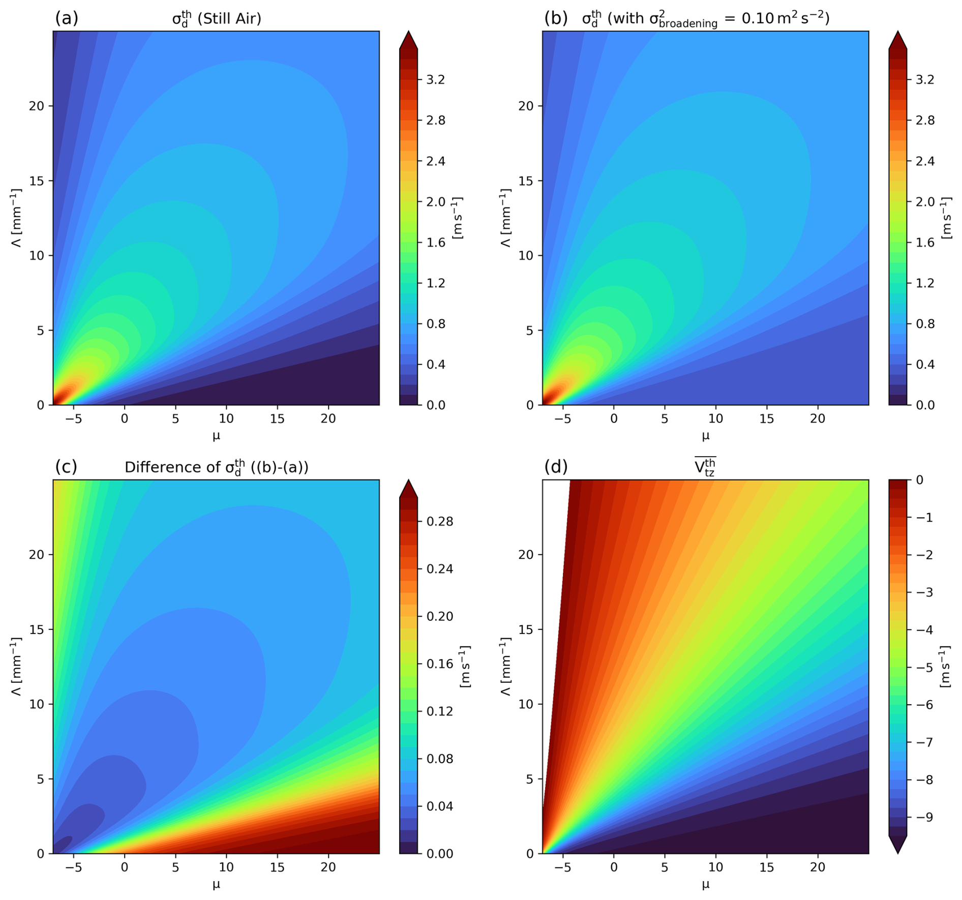
Figure 6 Theoretical values of (a) ${\mathit{\sigma }}_{\mathrm{d}}^{\mathrm{th}}$ in still air, (b) ${\mathit{\sigma }}_{\mathrm{d}}^{\mathrm{th}}$ when the broadening has a variance of 0.10 m² s⁻², (c) difference in ${\mathit{\sigma }}_{\mathrm{d}}^{\mathrm{th}}$ (b–a), and (d) $\stackrel{\mathrm{‾}}{V_{tz}^{\mathrm{th}}}$ with respect to combinations of μ and Λ obtained from scattering simulations using the T-matrix method. For this simulation, the wavelength is 32 mm, the raindrop temperature is 10 °C, the raindrop shape follows Thurai et al. (2007), D_max is 9 mm, D_min is 0.01 mm, and the calculation intervals for μ, Λ, and σ_broadening are set to 0.01. N₀ is set to 8000 mm${}^{-\mathrm{1}-\mathit{\mu }}$ m⁻³. The calculation ranges for μ and Λ are as shown in this figure, and σ_broadening is calculated from 0.00 (still air) to 1.19 m s⁻¹.

The procedure for estimating DSD parameters is described. The horizontal wind speed at altitude estimated using the VAD method is linearly interpolated to match the grid point heights of the NUX vertical observations, deriving the horizontal wind speed at each grid point. Additionally, we obtain the variance of ${\mathit{\sigma }}_{\mathrm{d}}^{\mathrm{NUX}}$ in vertical observations every 30 s for each altitude. Subsequently, ${\mathit{\sigma }}_{\mathrm{broadening}}^{\mathrm{2}}$ is obtained using Eqs. (9)–(12) and converted to standard deviation. This process yields the optimal σ_broadening for each time and altitude, enabling the search for DSD parameters thereafter.

For Z^∗nonRay, $\stackrel{\mathrm{‾}}{{V_{\mathrm{d}}}^{\mathrm{nonRay}}}$, $\stackrel{\mathrm{‾}}{V_{tz}^{\mathrm{nonRay}}}$, ${\mathit{\sigma }}_{\mathrm{d}}^{\mathrm{nonRay}}$, and ${\stackrel{\mathrm{‾}}{V}}_{\mathrm{a}}$ in Eqs. (6)–(8), the variables obtained from the observations in this study are expressed as Z^∗NUX, $\stackrel{\mathrm{‾}}{{V_{\mathrm{d}}}^{\mathrm{NUX}}}$, $\stackrel{\mathrm{‾}}{{V_{tz}}^{\text{NUX-MU}}}$ (or $\stackrel{\mathrm{‾}}{V_{tz}^{\mathrm{NUX}}})$, ${\mathit{\sigma }}_{\mathrm{d}}^{\mathrm{NUX}}$, and $\stackrel{\mathrm{‾}}{V_{\mathrm{a}}^{\mathrm{MU}}}$, respectively. First, one NUX profile is obtained as a 30 s value while the MU radar profile is derived as a 1 min value; thus, this study assumed that ${\stackrel{\mathrm{‾}}{V}}_{\mathrm{a}}$ remained the same for 1 min and the vertical profile of DSD parameters was estimated every 30 s. Second, the MU radar data are linearly interpolated to match the NUX grid points due to the difference in installation altitudes between the MU radar and the NUX (Tables 1 and 2). Third, Eq. (7) is transformed into the following equation to obtain $\stackrel{\mathrm{‾}}{{V_{tz}}^{\mathrm{NUX}-\mathrm{MU}}}$,

$$\begin{array}{}\text{(18)}& \stackrel{\mathrm{‾}}{{V_{tz}}^{\mathrm{NUX}-\mathrm{MU}}}=\stackrel{\mathrm{‾}}{V_{\mathrm{d}}^{\mathrm{NUX}}}-\stackrel{\mathrm{‾}}{V_{\mathrm{a}}^{\mathrm{MU}}}.\end{array}$$

Notably, only in Sect. 4.5, to confirm the importance of considering the effect of ${\stackrel{\mathrm{‾}}{V}}_{\mathrm{a}}$, similar to Rajopadhyaya et al. (1998), we also estimated the DSD parameters assuming $\stackrel{\mathrm{‾}}{V_{tz}^{\mathrm{NUX}}}=\stackrel{\mathrm{‾}}{V_d^{\mathrm{NUX}}}$.

Next, the optimal combination of μ and Λ that minimises the error is obtained using the least-squares method expressed in the following equation,

$$\begin{array}{}\text{(19)}& \begin{array}{rl}& O_{pt}\left(\mathit{\mu },\mathrm{\Lambda },{\mathit{\sigma }}_{\mathrm{broadening}}\right)\\ & ={\left\{\stackrel{\mathrm{‾}}{{V_{tz}}^{\mathrm{NUX}-\mathrm{MU}}}-\stackrel{\mathrm{‾}}{V_{tz}^{\mathrm{th}}}\left(\mathit{\mu },\mathrm{\Lambda }\right)\right\}}^{\mathrm{2}}\\ & +{\left\{{\mathit{\sigma }}_{\mathrm{d}}^{\mathrm{NUX}}-{\mathit{\sigma }}_{\mathrm{d}}^{\mathrm{th}}\left(\mathit{\mu },\mathrm{\Lambda },{\mathit{\sigma }}_{\mathrm{broadening}}\right)\right\}}^{\mathrm{2}}.\end{array}\end{array}$$

Thus, the optimal μ and Λ are estimated by comparing the observation with theoretical values to which the estimated broadening has been added (i.e., a forward modelling approach). Finally, combining Eqs. (1) and (6), N₀ is calculated using the optimal combination of μ and Λ and the following equation,

$$\begin{array}{}\text{(20)}& N_{\mathrm{0}}={\displaystyle \frac{Z^{\ast }{\mathit{\pi }}^{\mathrm{5}}{\left|K\right|}^{\mathrm{2}}}{{\mathit{\lambda }}^{\mathrm{4}}{\int }_{D_{\min }}^{D_{\max }}{\mathit{\sigma }}_{\mathrm{b}}\left(D\right)D^{\mathit{\mu }}{e}^{-\mathrm{\Lambda }D}\mathrm{d}D}}.\end{array}$$

Note that attenuation correction was not applied to the NUX vertical reflectivity data. Although cumulative attenuation introduces a slight artificial vertical gradient, the total two-way path attenuation is estimated to be about 1.2 dB over a 3 km path even at 40 dBZ ≈12 mm h⁻¹ (e.g., Fukao and Hamazu, 2014) assuming the DSD of Marshall and Palmer (1948). Given the NUX vertical resolution of 150 m, the attenuation difference between adjacent range bins is negligible relative to the measurement fluctuations. Thus, the attenuation effect would not significantly affect the analysis of the vertical variation of N₀.

Figure 6 shows a range of $-\mathrm{7}\le \mathit{\mu }\le \mathrm{25}$, whereas fitting a gamma distribution often imposes a limit on the range of μ values (e.g., Kirankumar et al., 2008; Dolan et al., 2018). In this study, only grid points for which the optimal values of μ derived from Eq. (19) were within the range of $-\mathrm{3}\le \mathit{\mu }\le \mathrm{15}$ were used in the analysis. This screening process removed about 1.4 % of the total data.

3.5 Methods for comparing the cloud physical quantities

The DSD parameters (N₀, μ, and Λ) are difficult to estimate directly and exactly from polarimetric parameters, especially in radars operating at high scanning speeds (Keat et al., 2016). Therefore, the cloud physical quantities (D₀, LWC, and N_w) aloft retrieved from the NUX and MU radar-based estimated DSD parameters were compared with the TANX data to confirm the validity of the vertical pointing observations in this study. Several methods have been proposed to estimate the D₀ and LWC aloft using polarimetric parameters obtained from X-band dual polarisation radars. For the estimation of D₀, Anagnostou et al. (2008), Kim et al. (2010), and Matrosov et al. (2005) expressed the following equations, respectively:

$$\begin{array}{}\text{(21)}& {\displaystyle }{D}_{\mathrm{0}}=\mathrm{0.5}+\mathrm{1.5}{Z}_{\mathrm{DR}}-\mathrm{0.4}{Z}_{\mathrm{DR}}^{\mathrm{2}}+\mathrm{0.03}{Z}_{\mathrm{DR}}^{\mathrm{3}},\text{(22)}& {\displaystyle }{D}_{\mathrm{0}}=\mathrm{0.79}+\mathrm{0.77}{Z}_{\mathrm{DR}},\text{(23)}& {\displaystyle }{D}_{\mathrm{0}}=\mathrm{1.46}{Z}_{\mathrm{DR}}^{\mathrm{0.49}}.\end{array}$$

For the estimation of LWC, Anagnostou et al. (2008) expressed the following equation:

$$\begin{array}{}\text{(24)}& \mathrm{LWC}={\mathrm{10}}^{-\mathrm{2.9}}{\left(Z^{\ast }\right)}^{\mathrm{2}}{\mathrm{10}}^{-\mathrm{2.48}{Z}_{\mathrm{DR}}+\mathrm{1.72}{Z}_{\mathrm{DR}}^{\mathrm{2}}-\mathrm{0.5}{Z}_{\mathrm{DR}}^{\mathrm{3}}+\mathrm{0.06}{Z}_{\mathrm{DR}}^{\mathrm{4}}}.\end{array}$$

Maki et al. (2005) also proposed equations to estimate LWC using DSD derived from disdrometer data observed in Japan, which were expressed as:

$$\begin{array}{}\text{(25)}& {\displaystyle }\mathrm{LWC}=\mathrm{0.00393}{\left(Z^{\ast }\right)}^{\mathrm{0.55}},\text{(26)}& {\displaystyle }\mathrm{LWC}=\mathrm{0.991}{K}_{\mathrm{DP}}^{\mathrm{0.713}}.\end{array}$$

Although K_DP is considered less sensitive and unreliable for small raindrops with small oblateness, Godo et al. (2014) found that the XRAIN K_DP is sensitive enough at 0.1 degree km⁻¹ or more. The K_DP used in the following analysis was confirmed to be greater than 0.1 degree km⁻¹; therefore, no sensitivity issues are expected. The N_w is expressed using the D₀ and LWC (e.g., Bringi and Chandrasekar, 2001) as follows:

$$\begin{array}{}\text{(27)}& N_{\mathrm{w}}={\displaystyle \frac{{\mathrm{3.67}}^{\mathrm{4}}}{\mathit{\pi }{\mathit{\rho }}_{\mathrm{w}}}}\left({\displaystyle \frac{\mathrm{1000}\mathrm{LWC}}{D_{\mathrm{0}}^{\mathrm{4}}}}\right),\end{array}$$

where ρ_w [g cm⁻³] is the density of liquid water (1 g cm⁻³).

The estimated DSD parameters, assuming a gamma distribution from vertical pointing observations, can also be used to obtain cloud physical quantities. The LWC is defined by the following equation (e.g., Fukao and Hamazu, 2014; Williams et al., 2016):

$$\begin{array}{}\text{(28)}& \mathrm{LWC}={\displaystyle \frac{\mathrm{0.001}\mathit{\pi }{\mathit{\rho }}_{\mathrm{w}}}{\mathrm{6}}}{\int }_{D_{\min }}^{D_{\max }}{D}^{\mathrm{3}}N\left(D\right)\mathrm{d}D.\end{array}$$

The D₀ is the raindrop diameter when the following equation is satisfied (Fukao and Hamazu, 2014):

$$\begin{array}{}\text{(29)}& \begin{array}{rl}& {\displaystyle \frac{\mathrm{0.001}\mathit{\pi }{\mathit{\rho }}_{\mathrm{w}}}{\mathrm{6}}}{\int }_{D_{\min }}^{D_{\mathrm{0}}}{D}^{\mathrm{3}}N\left(D\right)\mathrm{d}D\\ & ={\displaystyle \frac{\mathrm{0.001}\mathit{\pi }{\mathit{\rho }}_{\mathrm{w}}}{\mathrm{6}}}{\int }_{D_{\mathrm{0}}}^{D_{\max }}{D}^{\mathrm{3}}N\left(D\right)\mathrm{d}D.\end{array}\end{array}$$

According to Eq. (29), D₀ is the raindrop diameter that divides the total volume of raindrops into two equal halves. For the integral calculations in Eqs. (28)–(29), D_min, D_max, and the interval segments of D were set as in the scattering simulation in Sect. 3.4 (0.01 mm, 9 mm, and 1024 segments, respectively). For Eq. (29), D₀ was obtained by iteration when the difference between the left and right sides was minimised. N_w was obtained by substituting LWC and D₀ estimated from Eqs. (28)–(29) into Eq. (27). In this study, Eqs. (21)–(27) were applied to the TANX data and Eqs. (27)–(29) to the NUX data.

3.6 Estimation and comparison of dominant cloud microphysical processes

In this study, we attempt to infer the dominant cloud microphysical processes from the vertical variations of multiple cloud physical quantities derived from vertical pointing observations. For example, if there is no vertical variation in LWC, i.e., no condensation or evaporation, and D₀ increases (decreases) downward, collision-coalescence (breakup) is expected to be dominant. As Misumi et al. (2021) pointed out, N_w is likely to increase as the number of small raindrops increases. Based on this idea, N_w should decrease (increase) downward if collision-coalescence (breakup) is predominant because the number concentration of small raindrops should decrease (increase). If condensation (evaporation) is dominant, LWC increases (decreases) downward (e.g., Williams, 2016). When condensation (evaporation) is dominant, the number of small raindrops increases (decreases), so the value of N_w is expected to become larger (smaller). Notably, Williams (2016) similarly estimated the dominant cloud physical processes from vertical changes in cloud physical quantities; however, the difference between this study and Williams (2016) is that the latter used the total number of drops (N_t) instead of N_w. Using N_w in our discussion provides clearer insight into the behaviour of smaller raindrops. This study enables more robust discussion by confirming vertical variations in multiple cloud physical quantities.

The dominant cloud microphysical processes estimated from the vertical pointing observations were compared using TANX polarimetric parameters following the method of Kumjian and Prat (2014). Kumjian and Prat (2014) proposed a method to estimate the predominant warm cloud microphysical processes from the altitude variation of polarisation parameters. For example, if both the Z and Z_DR values increase (decrease) toward the lower layers, coalescence (breakup) should be dominant. We used only the PPI data of TANX at elevation angles of 2.5, 3.7, and 4.9° that are observed above the Shigaraki MU Observatory.

4 Results and discussion

4.1 Overview

This study focuses on a rainfall event that occurred on 2 June 2023 at the Shigaraki MU Observatory. Figure 7a–c and d–e are time–height cross sections of parameters obtained from NUX and MU radar observations, respectively. The tropospheric observation mode of the MU radar was from 09:40 to 16:59 JST (UTC + 9 h) on this day. As the 0 °C altitude on this day was roughly 4900 m according to the ERA5 data, only data at an altitude of about 3400 m or lower (liquid phase) were used. The black dots in Fig. 7 indicate the times that satisfy the criteria for typical stratiform rainfall defined in Sect. 3.2 and were used in the following analyses. Figure 7d and e show that stratiform precipitation was dominant, particularly during the second half of the MU radar observation period. Figure 7c shows that the reflectivity in typical stratiform rainfall was generally around 30 dBZ and occasionally exceeded 40 dBZ. In Fig. 7a, Doppler velocity values are negative for most of the time, and temporal fluctuations in the values can also be observed in the liquid phase. Figure 7b shows that during periods of typical stratiform rainfall, the fluctuations in ${\mathit{\sigma }}_{\mathrm{d}}^{\mathrm{NUX}}$ are smaller compared to other periods. Note that the data shown in Fig. 7a–c correspond to the short pulse region. Additionally, Fig. 8 shows the 1 km-mesh synthetic radar grid point value (precipitation intensity [mm h⁻¹]) provided by the Japan Meteorological Agency (JMA) for the constant altitude plan position indicator (CAPPI) at the 2 km level at 14:40 JST, when stratiform precipitation and large Z^NUX values were observed (Fig. 7c). This rainfall event featured an active stationary front, with strong convective precipitation distributed generally in the southern part of the precipitation system, and surrounding stratiform precipitation (Fig. 8).

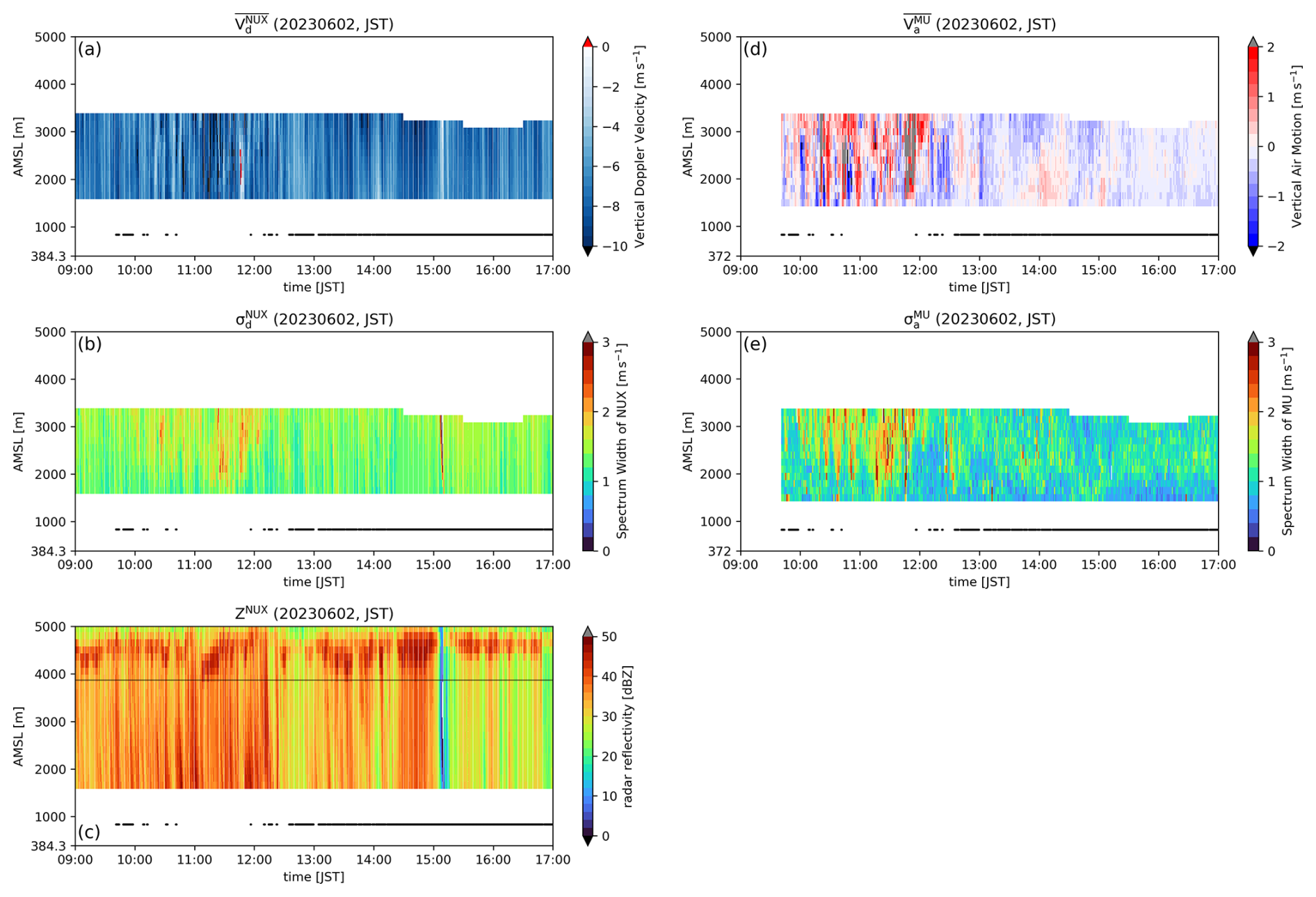
Figure 7 Time–height cross sections of (a) $\stackrel{\mathrm{‾}}{{V_{\mathrm{d}}}^{\mathrm{NUX}}}$, (b) ${\mathit{\sigma }}_{\mathrm{d}}^{\mathrm{NUX}}$, (c) Z^NUX, (d) $\stackrel{\mathrm{‾}}{V_{\mathrm{a}}^{\mathrm{MU}}}$, and (e) ${\mathit{\sigma }}_{\mathrm{a}}^{\mathrm{MU}}$ for the analysis period, 09:40 to 16:59 JST (Japan Standard Time, UTC + 9 h), on 2 June 2023. The black dots at the bottom of panels (a)–(e) indicate times when the criteria for “typical stratiform rainfall” defined in Sect. 3.2 are satisfied. The shading in (a)–(c) shows only the periods for which vertical pointing observations were performed. The shading in (a)–(b) and (d)–(e) indicates only the specific altitude data used for the analysis. In (a) and (d), positive values represent upward motion and negative values represent downward motion. The grey horizontal line in (c) indicates the maximum beam altitude over the Shigaraki MU Observatory when observed by TANX at an elevation angle of 4.9°.

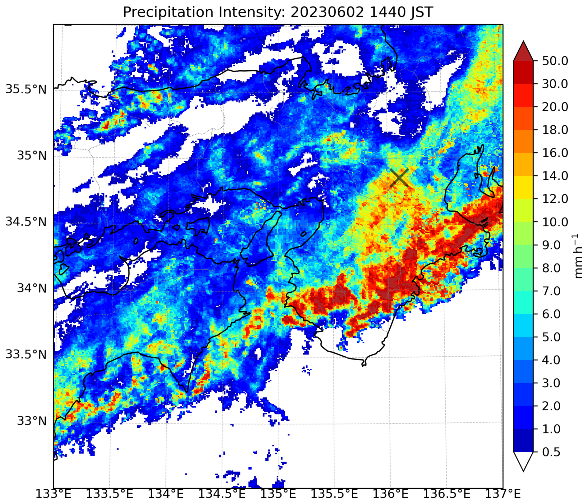
Figure 8 Precipitation intensity at the 2 km level at 14:40 JST on 2 June 2023, using the 1 km mesh synthetic radar grid (C-band radar network) data provided by the JMA. The grey × mark indicates the location of the Shigaraki MU Observatory.

We use TANX data for comparison with vertical observations. The TANX data used in the following analysis include only the data from times when typical stratiform rainfall was identified by the MU radar for at least 4 min out of 5 min. In this analysis, 52 TANX volume scan datapoints were used. Figure 9 shows time-height cross sections of TANX data just above the Shigaraki MU Observatory. Note that only the data from the lower three layers in Fig. 9 are used in this study. The temporal and altitude variations in radar reflectivity are generally consistent between Figs. 7c and 9a; for example, both show relatively strong radar reflectivity around 14:40 JST. In some cases, the temporal and vertical variations of $Z_{\mathrm{DR}}^{\mathrm{TANX}}$ and $K_{\mathrm{DP}}^{\mathrm{TANX}}$ correspond to changes in Z^TANX; for example, around 14:40 JST, both $Z_{\mathrm{DR}}^{\mathrm{TANX}}$ and $K_{\mathrm{DP}}^{\mathrm{TANX}}$ tend to increase as Z^TANX increases (Fig. 9). Notably, from 13:00 to 14:00 JST, the high-reflectivity area interpreted as the melting layer decreased in altitude to around 3500 m (Fig. 9a). However, vertical observations show no indication that the melting layer altitude decreased to around 3500 m (Fig. 7c). Instead, considering the beam broadening of TANX, the beam at an elevation angle of 4.9° may intermittently capture the lower edge of the melting layer (Fig. 7c), potentially causing an enhancement in radar reflectivity (Fig. 9a). Data at an elevation angle of 4.9° are used throughout this analysis, although they might be affected by the melting particles.

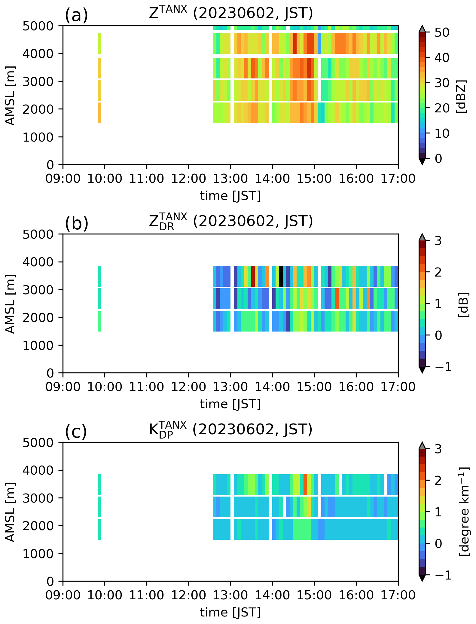
Figure 9 Time–height cross sections of (a) Z^TANX, (b) $Z_{\mathrm{DR}}^{\mathrm{TANX}}$, and (c) $K_{\mathrm{DP}}^{\mathrm{TANX}}$ for the analysis period, 09:40 to 16:59 JST, on 2 June 2023. The data are processed as PPI data. Data are from the lower layer at elevation angles of 2.5, 3.7, 4.9, 6.2, and 7.5°. Note that the shading in (b)–(c) indicates only the specific altitude data used for the analysis (only 2.5, 3.7, and 4.9°).

4.2 Retrieval of DSD parameters

Figure 10 shows the contoured frequency by altitude diagrams (CFADs; Yuter and Houze, 1995) of the DSD parameters at the times identified as typical stratiform rainfall. Figure 10d exhibits a decreasing number of grid points at higher altitudes, which is due to the effect of variations in the 0 °C altitude between 09:40 and 16:59 JST. Figure 10a and b show that the values of μ and Λ generally increase with decreasing altitude except for the highest altitude; the median of μ changes from −0.31 at 3160 m to 1.21 at 1660 m, and the median of Λ changes from 3.34 to 4.22. This trend is the same as that described by Rao et al. (2006) and Kirankumar et al. (2008) for stratiform precipitation and is also consistent with the trend of the μ–Λ relationship derived in previous studies (e.g., Rao et al., 2006; Wen et al., 2020). The present case has smaller median values for both μ and Λ than those reported by Rao et al. (2006) and Kirankumar et al. (2008), suggesting that this case has a wider range of raindrop sizes; i.e., it contains a variety of raindrops from small to large in diameter. N₀ is a parameter whose units vary with the value of μ, and Fig. 10c shows that N₀ increases as μ increases toward lower altitudes except for the highest altitude.

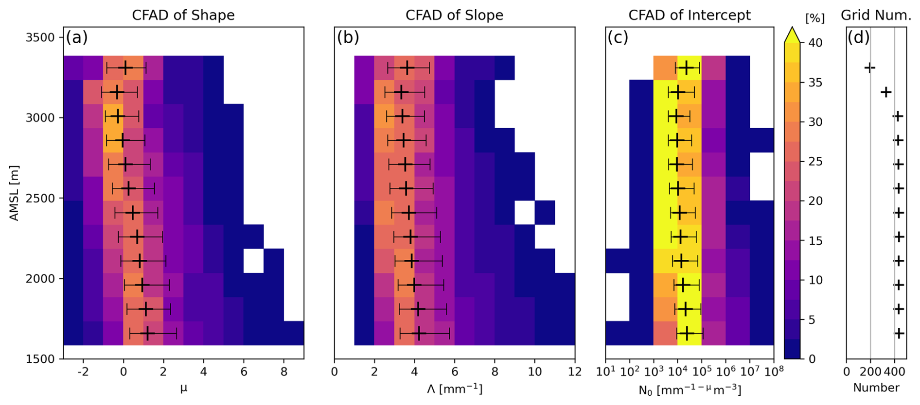
Figure 10 CFADs for (a) μ, (b) Λ, and (c) N₀ at the times determined to be typical stratiform rainfall. The + marks and bars in (a)–(c) indicate the median and interquartile range, respectively, for each altitude. The + marks in (d) indicate the number of grid points analysed for each altitude. The vertical interval is 150 m for (a) to (d).

Figure 11 shows the DSD using the median values of μ, Λ, and N₀ for each altitude shown in Fig. 10. The number concentrations of both small and large particles tend to decrease with decreasing altitude (Fig. 11a and d). On the other hand, the number concentration of intermediate size particles (around 1.5 mm) increases with decreasing altitude (Fig. 11b and c). Thus, the width of the DSD tends to narrow as the altitude decreases in this case.

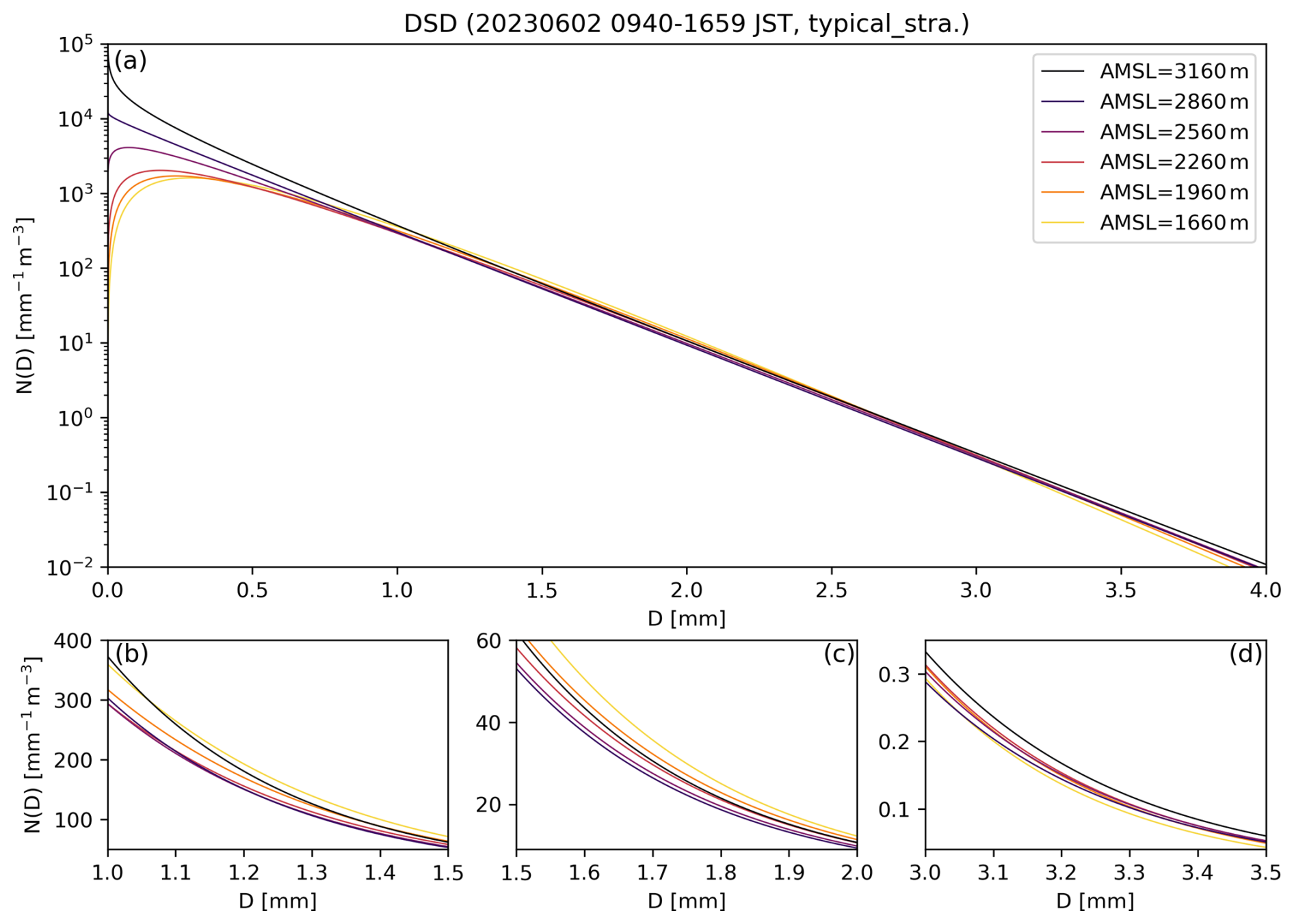
Figure 11 (a) DSD using the median values of μ, Λ, and N₀ for each altitude; (b–d) enlarged views of the diameter ranges (b) 1.0–1.5 mm, (c) 1.5–2.0 mm, and (d) 3.0–3.5 mm. The vertical axes are (a) logarithmic and (b–d) linear. For better visualisation, the altitude levels are thinned out.

4.3 Comparison of the retrieved cloud physical quantities

Figure 12 presents the altitude variation of the estimated median D₀, LWC, and N_w retrieved from the NUX and MU radar vertical observations and from TANX PPI scans. Notably, the data from the vertical observations are every 30 s, while the TANX conducts one volume scan every 5 min. Figure 12a shows that the D₀ estimated from NUX and MU radar observations (magenta + marks; Eq. 29) was generally within the range of D₀ estimated using Z_DR (Eqs. 21–23), although it was slightly larger than that estimated by the method of Kim et al. (2010) below 2300 m. Fig. 12b shows similarity in the vertical variation trends between the LWC estimated from NUX and MU radar vertical observations (magenta + marks; Eq. 28) and that from TANX using K_DP (blue dots; Eq. 26), although the former exhibits larger values. In addition, the N_w estimated from vertical observations (magenta + marks; Eq. 27) and that using LWC estimated from K_DP (blue dots) roughly agreed (Fig. 12c). The slight discrepancy in N_w above 2600 m (Fig. 12c) could be attributed to the fact that D₀ estimated by vertical observation is smaller than that estimated when the method described by Kim et al. (2010; Eq. 22) was used to calculate N_w (blue dots; Eq. 27). However, the D₀ estimated from the vertical observations is close to that estimated by the method of Anagnostou et al. (2008; Eq. 21) above 2600 m, suggesting that its fluctuations can be estimated with reasonable accuracy.

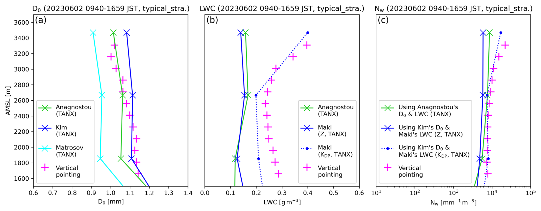
Figure 12 Comparison of the median values for each altitude of the parameters (a) D₀, (b) LWC, and (c) N_w. The green, blue, and cyan marks are parameters derived from Eqs. (21)–(27) using TANX PPI data. The magenta + marks are parameters derived from Eqs. (27)–(29) using vertical observation data.

Maki et al. (2005) showed the error range of Eq. (26) (blue dots in Fig. 12b) using the normalised mean absolute error, indicating that when LWC is around 0.25 g m⁻³, the error is approximately ±0.07 g m⁻³. The absolute difference between the median LWC estimated from the K_DP of TANX and that estimated from the vertical observations (linearly interpolated to the TANX altitudes) is about 0.06 g m⁻³ at 1850 m a.m.s.l. and about 0.05 g m⁻³ at 2660 m a.m.s.l. This means that the difference between the LWC estimated from vertical observations and that estimated using the K_DP of TANX is within the error range specified in Eq. (26). Furthermore, when K_DP is simulated using the T-matrix method with DSD parameters obtained from vertical observations, the median values of K_DP are 0.11 degree km⁻¹ at both 1810 and 2710 m (Fig. 13). The median K_DP value for the nearest grid point using TANX is also 0.11 degree km⁻¹ at both heights. Thus, the difference between the DSD used by Maki et al. (2005) and the DSD retrieved in this study may be considered to cause the discrepancy in the estimated LWC.

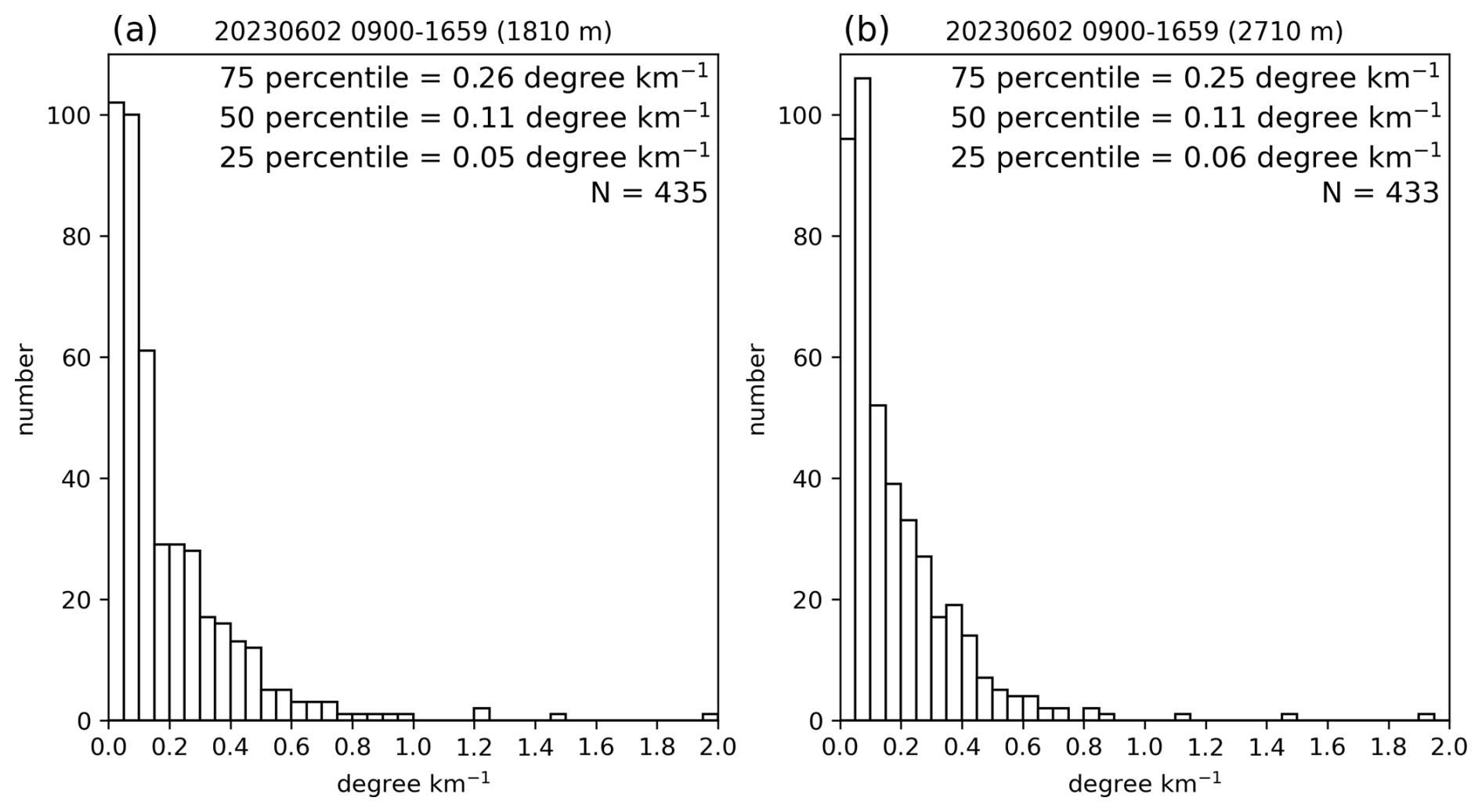
Figure 13 Histograms of K_DP calculated using the T-matrix method from DSD estimated from vertical observations, (a) at 1810 m and (b) at 2710 m. N is the total number of samples.

LWC estimated from Z^∗ (Eqs. 24–25) differed significantly from that estimated using vertical observations (Eq. 28) and K_DP (Eq. 26; Fig. 12b), not only in its values but also in its vertical variation trend. The sensitivity of Z^∗ and K_DP to DSD variations is discussed. The nth order moment of DSD is defined by the following equation (e.g., Fukao and Hamazu, 2014),

$$\begin{array}{}\text{(30)}& m_n\equiv {\int }_{\mathrm{0}}^{\mathrm{\infty }}{D}^{n}N\left(D\right)\mathrm{d}D.\end{array}$$

Assuming the Rayleigh scattering approximation, Z^∗ is the 6th moment of DSD from Eq. (2) and K_DP is the 4.3–4.9 moment (Ryzhkov and Zrnic, 2019). On the other hand, LWC is represented by the 3rd moment from Eq. (28). Thus, Z^∗ is a higher-order moment than K_DP and has higher sensitivity to DSD variations, making LWC estimations derived from Z^∗ susceptible to errors due to DSD variations.

In addition, Z and Z_DR are considered to be affected by attenuation, although the attenuation correction of Z^TANX and $Z_{\mathrm{DR}}^{\mathrm{TANX}}$ is performed using $K_{\mathrm{DP}}^{\mathrm{TANX}}$ following Maesaka et al. (2011). Notably, horizontal specific attenuation (A_h [dB km⁻¹]) is less sensitive to raindrop shape than specific differential attenuation (A_DP [dB km⁻¹]; Ryzhkov and Zrnic, 2019). This means that A_h is also more susceptible to the effects of small raindrops, to which K_DP is insensitive. Consequently, the attenuation correction for Z^TANX is especially likely to be underestimated in weak rainfall, and the error may increase over about 38 km of rain path. As A_h is more susceptible to variations in DSD than A_DP (Ryzhkov and Zrnic, 2019), the error in Z is likely to be larger than that in Z_DR.

Overall, the D₀, LWC, and N_w estimated from the vertical observations in this study are broadly consistent with those estimated using K_DP and Z_DR (Fig. 12). Therefore, the cloud physical quantities estimated from vertical observations can be considered reliable.

4.4 Confirming the influence of ${\mathit{\sigma }}_{\mathrm{d}}^{\mathrm{NUX}}$ broadening

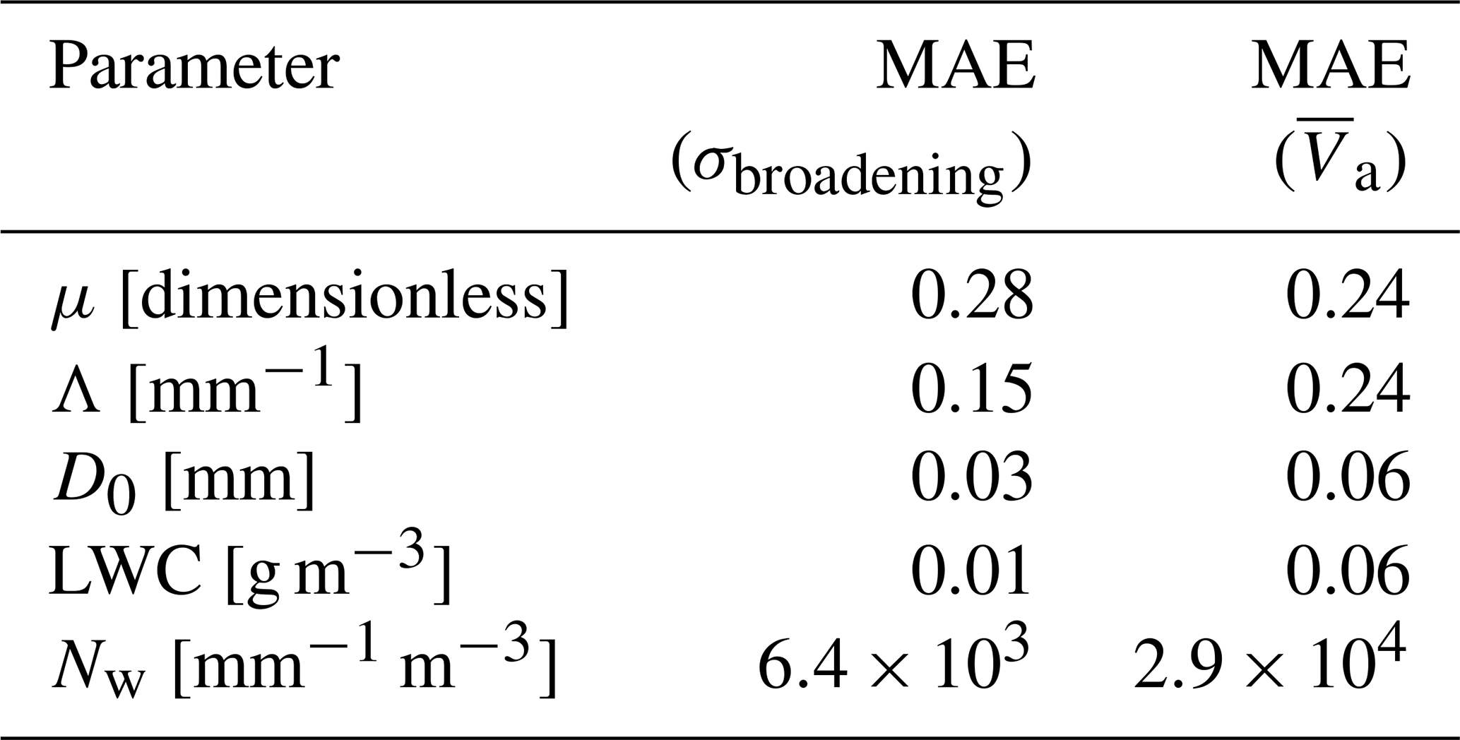
We discuss the broadening effect on ${\mathit{\sigma }}_{\mathrm{d}}^{\mathrm{NUX}}$. Figure 14 shows the differences in DSD parameters and cloud physical quantities estimated at each altitude with and without the removal of the influence of σ_broadening. We focus particularly on μ. The mean absolute error (MAE) for μ is 0.28 (Table 4). As shown in Fig. 14a, the values of the interquartile range (IQR) of μ vary between 2 and 3 at all altitudes. The MAE represents about 10 % of the IQR, and since the Wilcoxon test revealed significant differences in all layers, systematic shifts in the distribution are indicated. Given that μ is a sensitive shape parameter governing the curvature of the DSD, a systematic bias equivalent to 10 % of the natural variability can lead to non-negligible errors in derived microphysical properties. The statistical significance further confirms that this correction removes a persistent bias, thereby improving the quantitative accuracy of the retrieval. Therefore, even during the typical stratiform rainfall period defined in this study, σ_d correction remains important.

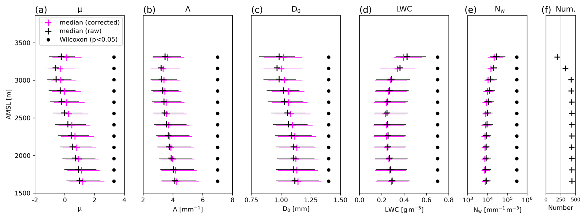
Figure 14 Comparison of (a–b) DSD parameters and (c–e) cloud physical quantities estimated (magenta) with the correction for the influence of σ_broadening and (black) without the correction. Note that the correction using $\stackrel{\mathrm{‾}}{V_{\mathrm{a}}^{\mathrm{MU}}}$ is performed for both magenta and black. (f) indicates the sample size. For each altitude, the + marks indicate the median, and the bars represent the interquartile range (IQR). Black circles at each altitude indicate significant differences (p<0.05) detected by the Wilcoxon signed-rank test.

Table 4 Mean absolute error (MAE) for each parameter when comparing cases with and without correction for the influence of σ_broadening and ${\stackrel{\mathrm{‾}}{V}}_{\mathrm{a}}$.

4.5 Confirming the influence of ${\stackrel{\mathrm{‾}}{V}}_{\mathrm{a}}$

This section evaluates the influence of ${\stackrel{\mathrm{‾}}{V}}_{\mathrm{a}}$ on DSD estimation. Figure 15 shows the differences in DSD parameters and cloud physical quantities estimated at each altitude when the influence of ${\stackrel{\mathrm{‾}}{V}}_{\mathrm{a}}$ is removed, as in Eq. (18), or when assuming $\stackrel{\mathrm{‾}}{V_{tz}^{\mathrm{NUX}}}=\stackrel{\mathrm{‾}}{V_{\mathrm{d}}^{\mathrm{NUX}}}$. Figure 15 indicates that significant differences are present in Wilcoxon's signed-rank test for all parameters and at almost all altitudes. The MAE for both μ and Λ is 0.24 (Table 4), which corresponds to approximately 10 % of the IQR (Fig. 15). Furthermore, the influence of ${\stackrel{\mathrm{‾}}{V}}_{\mathrm{a}}$ correction on D₀, LWC, and N_w evaluated by MAE is larger than that of σ_d correction. This fact demonstrates that even during typical stratiform rainfall characterised by a small $\left|{\stackrel{\mathrm{‾}}{V}}_{\mathrm{a}}\right|$ $\left(\left|\stackrel{\mathrm{‾}}{V_{\mathrm{a}}^{\mathrm{MU}}}\right|\le \mathrm{1.0}{\mathrm{m}\mathrm{s}}^{-\mathrm{1}}\right)$, ${\stackrel{\mathrm{‾}}{V}}_{\mathrm{a}}$ has a significant influence on the estimation of DSD parameters and cloud physical quantities. Therefore, when estimating DSD from vertical observations, the retrieval of ${\stackrel{\mathrm{‾}}{V}}_{\mathrm{a}}$ needs to be performed carefully and accurately.

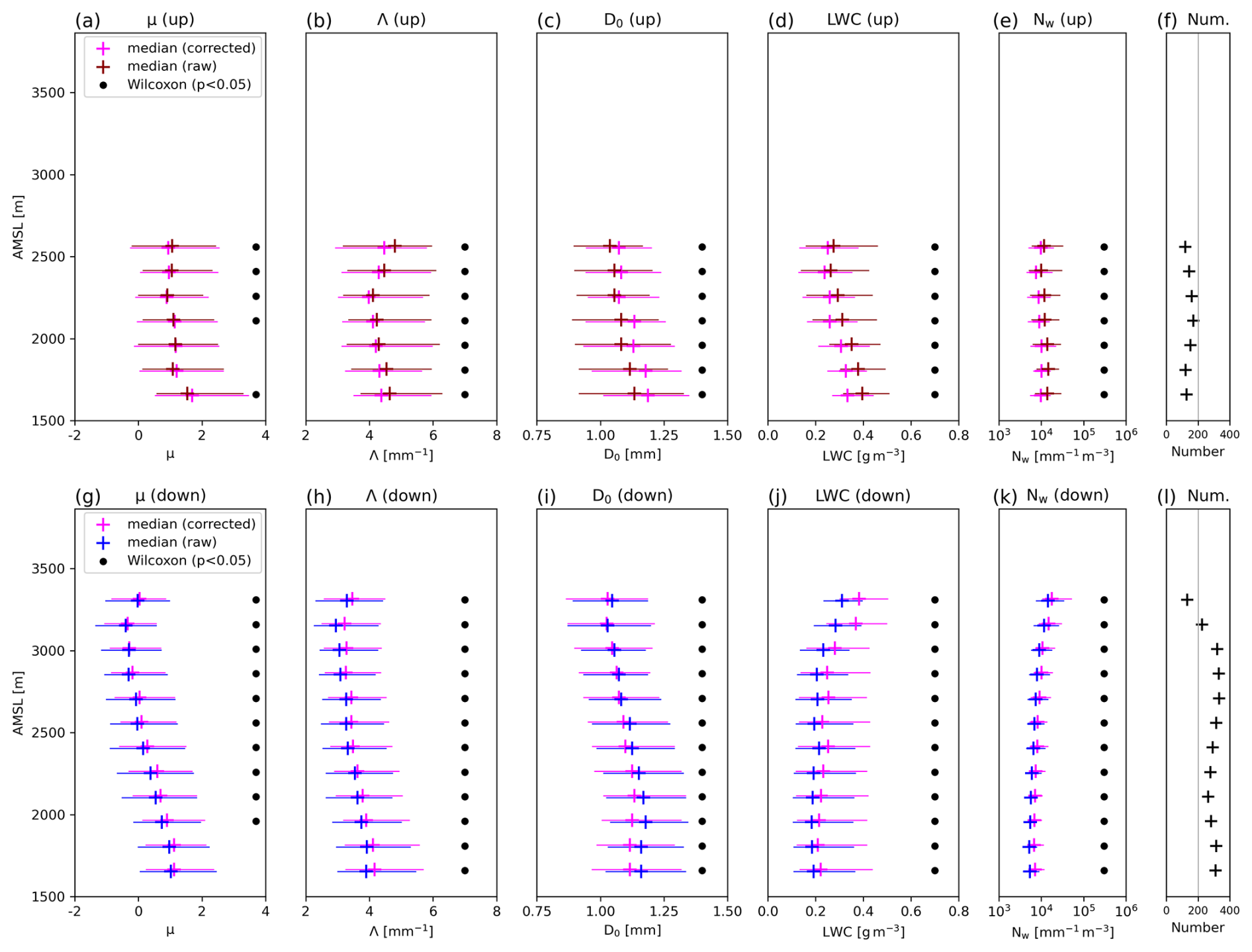
Figure 15 The same as Fig. 14, but comparing estimates with ${\stackrel{\mathrm{‾}}{V}}_{\mathrm{a}}$ correction using $\stackrel{\mathrm{‾}}{V_{\mathrm{a}}^{\mathrm{MU}}}$ and those without the correction indicated by dark red or blue marks. The panels show the cases for (a)–(f) when $\stackrel{\mathrm{‾}}{V_{\mathrm{a}}^{\mathrm{MU}}}\ge \mathrm{0}$, i.e., upward air motion, and for (g)–(l) when $\stackrel{\mathrm{‾}}{V_{\mathrm{a}}^{\mathrm{MU}}}<\mathrm{0}$, i.e., downward air motion. Note that the σ_d correction is performed in all estimates. (f) and (l) indicate the sample size, and only cases with 100 or more samples per altitude are plotted in all panels.

Based on the discussions in this section and Sect. 4.4, even in typical stratiform rainfall, the estimation of DSD is susceptible to the effects of vertical air motion, horizontal wind, and turbulence. Therefore, accurate DSD estimation without raw Doppler spectra requires data correction as performed in previous studies (e.g., Shupe et al., 2008; Williams et al., 2016; Pang et al., 2021) and this study. This fact is considered applicable to the Ku-band satellite-borne Doppler radar, which operates at a frequency close to that of X-band radar, suggesting that accurate DSD estimation using pulse-pair Doppler processing could be achieved if vertical air motion is accurately retrieved and horizontal wind is derived using along-track and cross-track techniques.

4.6 Estimation and validation of cloud microphysical processes derived from vertical pointing observations

The estimated DSD parameters and cloud physical quantities vary with altitude (Figs. 10 and 12), and the cloud microphysical processes responsible for their variations are discussed. At altitudes between 3010 and 1660 m, the overall variation in LWC values derived from vertical pointing observations is relatively small (0.24–0.29 g m⁻³; Fig. 12b). This indicates that condensation and evaporation are minimal at these altitudes. Between altitudes of 3010 and 2110 m, D₀ tends to increase (from 1.00 to 1.13 mm) and N_w tends to decrease (from 10900 to 7600 mm⁻¹ m⁻³) toward the lower altitudes (Fig. 12a and c), suggesting that the collision-coalescence of raindrops is predominant. At altitudes below 2110 m, the changes in D₀ and N_w with altitude are slight, with variation in D₀ from 1.13 to 1.14 mm and the range of N_w being from 7300 to 7800 mm⁻¹ m⁻³. This may be approaching the equilibrium shape of DSD, which is characterised by simultaneous coalescence and breakup due to collisions among raindrops (Zawadzki and De Agostinho Antonio, 1988). Notably, equilibrium DSD is often expressed as a bimodal (e.g., McFarquhar, 2004; Okazaki et al., 2023; Unuma, 2024) or trimodal (e.g., Chen and Lamb, 1994) distribution, and such distributions cannot be expressed using a gamma distribution. However, vertical one-dimensional numerical simulations by Barthes and Mallet (2013) have shown that μ and Λ tend to increase downward as equilibrium shape is approached through collision-coalescence and breakup. The DSD in this study (Figs. 10 and 11) may also be approaching equilibrium shape downward. This is because, despite median μ and Λ increasing below an altitude of 2110 m (from 0.81 to 1.21 and from 3.86 to 4.22 mm⁻¹, respectively), the changes in D₀ and N_w are minimal (Fig. 12a and c). At altitudes above 3010 m, LWC and N_w obtained from vertical pointing observations decrease downward (Fig. 12b and c), suggesting that evaporation of small raindrops may be dominant. At these altitudes, D₀ increases or decreases slightly (Fig. 12a). In particular, a decreasing D₀ is not the behaviour generally expected in conditions where evaporation is predominant (Xie et al., 2016). However, Xie et al. (2016) also show that special cases exist in which D₀ decreases downward due to evaporation in the region where the initial μ≈0. As the median value of μ at the highest altitude analysed in this case is 0.10 (Fig. 10a), these special fluctuations in D₀ might have been caused by evaporation. Therefore, in this analysis, collision-coalescence is considered to have contributed the most, with breakup and evaporation also contributing.

The verification of the dominant cloud microphysical processes inferred from vertical observations is performed using TANX data. Figure 16 shows the predominant cloud microphysical processes in the liquid phase estimated from the method of Kumjian and Prat (2014) using TANX data. From Fig. 16, collision-coalescence and breakup are dominant most of the time, followed by signals of evaporation and size-sorting. This is generally consistent with the dominant cloud microphysical processes estimated from vertical observations. This finding shows that dominant cloud microphysical processes can be estimated from the altitude variations of multiple cloud physical quantities derived from DSD parameters retrieved from vertical observations.

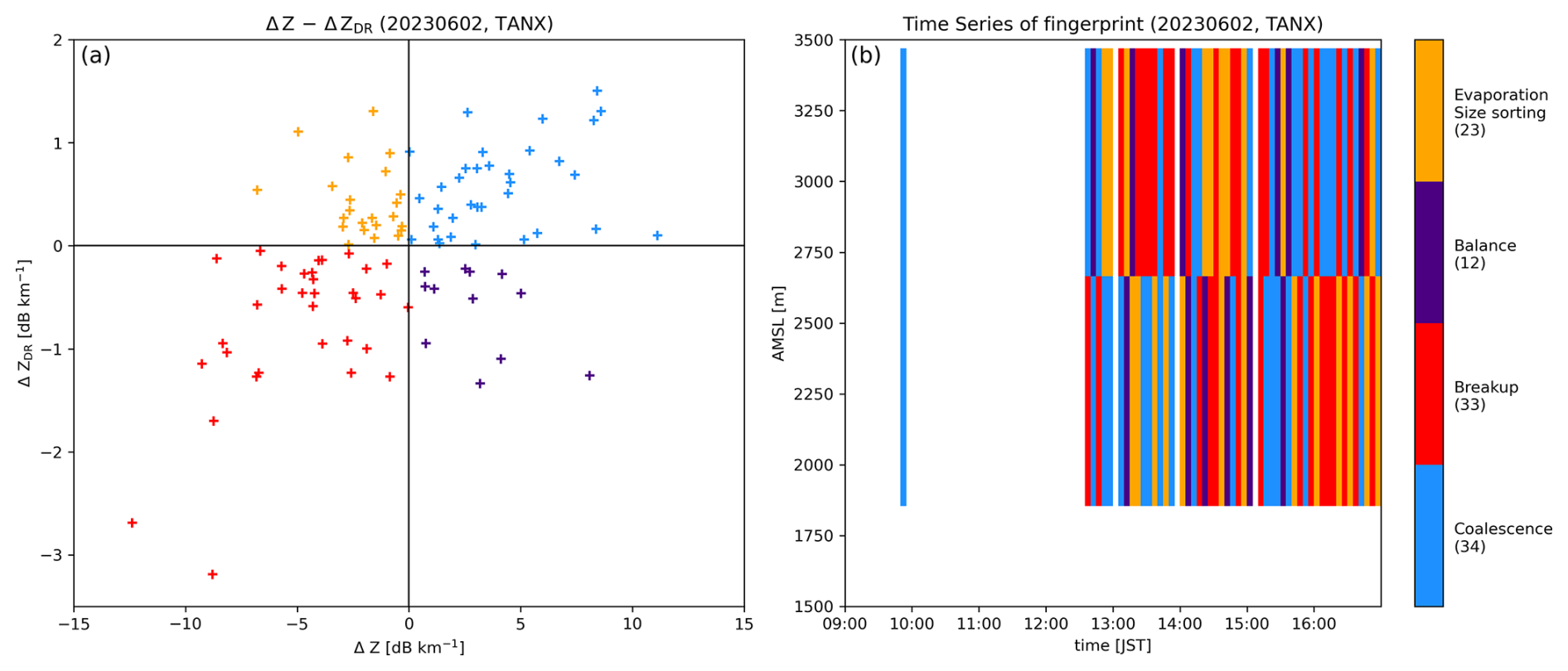
Figure 16 Using TANX data, the fingerprints of cloud microphysical processes in warm rain are shown in (a) the ΔZ–ΔZ_DR plane with decreasing altitude, and (b) the time-height cross section. The colours of the plots and shades correspond to the legend, and the numbers in the legend represent the number of data points for each category.

From the above discussion, the altitude variations of μ and Λ in Fig. 10 are primarily attributed to collision-coalescence and breakup. This perspective differs from the factors described by Rao et al. (2006) and Kirankumar et al. (2008) for DSD altitude variations in the tropics. This difference should be related to the relative humidity below the melting layer. Kirankumar et al. (2008) inferred a significant contribution from evaporation based on the results of numerical simulations (Ferrier et al., 1996), which indicate that evaporation contributes to continental precipitation at altitudes below the melting layer. However, in this analysis, the relative humidity in the ERA5 reanalysis data exceeded 75 % for most of the period at the analysed altitude (Fig. 17), indicating that the area below the melting layer is moist (e.g., Nishii et al., 2025). These moist conditions should have prevented the evaporation of the small-sized raindrops and increased the opportunities for collision-coalescence and collision-breakup between small and large raindrops.

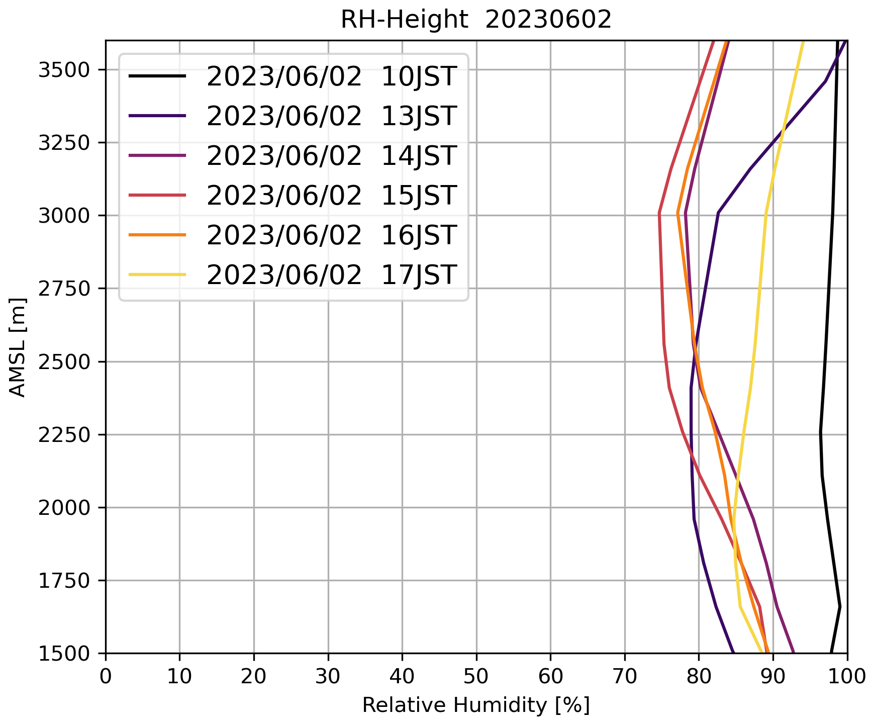
Figure 17 Vertical profiles of relative humidity over the Shigaraki MU Observatory are shown at each time. Only the data closest to the time depicted in the fingerprint in Fig. 16b are presented.

5 Summary

In this study, we introduce a method to estimate the vertical profile of DSD parameters and retrieve cloud physical quantities using vertical pointing observation data from X- and VHF-band radars, and apply it to a typical stratiform rainfall case in Japan. As NUX does not output raw spectra, the DSD estimation method proposed by Fukao and Hamazu (2014) utilising Doppler spectral width σ_d was used. Additionally, it was modified to account for non-Rayleigh effects using T-matrix method simulations. Even during periods of typical stratiform rainfall, contamination by ${\stackrel{\mathrm{‾}}{V}}_{\mathrm{a}}$ and σ_broadening in the estimation of DSD parameters and cloud physical quantities is shown to be non-negligible. This indicates that even under the calmest stratiform rainfall conditions, accurate DSD estimation requires correction for the effects of vertical air motion, horizontal wind, and turbulence. Additionally, this fact might indicate the challenges involved in applying DSD analysis to satellite Doppler radar. However, for rainfall that satisfies the conditions for typical stratiform rainfall defined in this study, the broadening effect of σ_d due to wind shear can be neglected even with radar having a vertical resolution of approximately 150 m. We also confirm that the cloud physical quantities retrieved using the DSD estimated from vertical observations are reasonably accurate.

The μ and Λ estimated from vertical pointing observations generally increase with decreasing altitude. The estimated vertical variations in cloud physical quantities (D₀, LWC, and N_w) suggest that collision-coalescence is the main factor causing vertical variations in these DSD parameters, with some influence from breakup and evaporation. The dominant cloud microphysical processes were also confirmed by applying the method of Kumjian and Prat (2014) to TANX data, and were generally consistent with vertical pointing observations. These results indicate that the contributing cloud microphysical processes are different, although the altitude variations of μ and Λ are similar to those in previous studies in the tropics (Rao et al., 2006; Kirankumar et al., 2008). The moist environment probably prevented the evaporation of small raindrops in this study.

This study demonstrates that combining the vertical variations of multiple cloud physical quantities enables the estimation of dominant cloud microphysical processes. We conclude that accurate estimation based solely on the vertical variation of DSD parameters or that of one cloud physical quantity, as performed in previous studies, is difficult. As changes in cloud physical quantities directly reflect cloud microphysical processes, we show that the accurate estimation of cloud microphysical processes can be achieved by combining multiple vertical variations in cloud physical quantities, such as D₀, LWC, and N_w. This study suggests that significant advances in the understanding of cloud microphysics can be achieved by interpreting the vertical variations in estimated DSD parameters in the context of the dominant cloud microphysical processes using only data from vertical pointing observations.

The vertical observations of NUX at the Shigaraki MU Observatory were performed until November 2025. This method will be used to conduct statistical analyses of the DSD for the rainy season in Japan.