Towards retrieving cloud top entrainment velocities from MISR cloud motion vectors

Although important, direct retrievals of entrainment rates in cloud-topped planetary boundary layer (PBL) remain elusive. Here we present a novel technique for retrieving cloud-top entrainment velocities using only Multi-angle Imaging Spectro-Radiometer (MISR) stereoscopic retrievals of cloud-motion vectors (CMVs) and cloud-top heights (CTHs). Mesoscale vertical air velocity at CTH is diagnosed from the continuity equation and then used to derive entrainment velocities from the PBL mass-budget equation. The algorithm is demonstrated through a case of marine stratocumulus deck off the California coast, with comparisons made against data from the European Centre for Medium-range Weather Forecasts (ECMWF) reanalysis (ERA5) and the data from other satellites. MISR low-cloud CTH for this case were lower than the ERA5 reported PBL depth by 189 ± 87 m. These differences in cloud top heights partly modulate the differences in the ERA5 and MISR horizontal winds, with larger differences in meridional over zonal wind components. Average difference between ERA5 and MISR derived mesoscale vertical air motion at cloud top was 0.14 ± 0.73 cm s⁻¹, while the same for entrainment rate was −0.09 ± 0.46 cm s⁻¹. The uncertainties in the utilized CTHs and CMVs are propagated to derive systematic and random retrieval uncertainties. Fractional uncertainty is lower than 25 % when the retrieved mesoscale vertical air motion is stronger than ±0.04 cm s⁻¹ and entrainment velocities are stronger than ±0.03 cm s⁻¹. These results showcase the ability to derive mesoscale vertical air motion and entrainment rates from MISR observations and motivate its extension to generate a global climatology leveraging its full 23-year record (2000–2022). Nonetheless comprehensive validation of the retrievals is warranted through comparisons with estimates from an independent dataset across diverse weather conditions.

1 Introduction

Boundary layer cumulus and stratocumulus clouds are routinely observed over land and oceans from the tropics to the poles. As these clouds reflect more solar radiation to space compared to the underlying surface, they exert a strong radiative influence on Earth's atmosphere (Wood, 2012; Klein and Hartmann, 1993; Bony and Dufresne, 2005). These low clouds are intimately coupled to the turbulence in the planetary boundary layer (PBL) that is modulated by surface fluxes, cloud top radiative cooling, wind shear and cloud top entrainment mixing (Bretherton et al., 2007; Moeng et al., 2005; Mellado et al., 2014; Wood, 2012; de Lozar and Mellado, 2017; Stevens, 2005). The mixing of the warm and dry air from above the cloud top into the cloud layer termed as entrainment, plays a crucial role in modulating cloud microphysical and radiative properties, thereby controlling cloud lifetime (Ackerman et al., 2004; Bretherton et al., 2007; Stevens, 2005; Wood, 2012; Eastman and Wood, 2018). The effects of entrainment mixing on PBL and cloud properties have been vastly debated and remain challenging to accurately represent in Earth System Models (ESM) and operational weather models (Nam et al., 2012; Vial et al., 2013). Recent studies have also shown entrainment mixing to modulate the responses of cloud and rain properties to changes in background aerosol concentrations (Grosvenor et al., 2018; Xu et al., 2022; Luo et al., 2020). Despite its importance, largely due to the difficulty in measuring, there have been few observations of entrainment rates, especially over remote oceanic regions.

As entrainment happens at very fine spatial (less than 10 m) and temporal (1–10 s) scales, the entrainment rates need to be derived from high resolution measurements (de Lozar and Mellado, 2017; Mellado, 2017). Observations of conserved variables and vertical air motion from a level leg at the cloud top have been used to derive entrainment velocities (Faloona et al., 2005; Gerber et al., 2013; Malinowski et al., 2013). However, these estimates suffer from sampling bias, are sporadic, and are cost intensive. In addition, they can be only made from slow moving airborne platforms like the Twin Otter or unmanned aerial systems (UAS) (Gerber et al., 2013; Norgren et al., 2016; Sorooshian et al., 2018; Lappin et al., 2024; Martin et al., 2014). Entrainment rates can also be retrieved from estimates of turbulence kinetic energy (TKE) derived from observations made by cloud radars (Albrecht et al., 2016; Shupe et al., 2012; Borque et al., 2016). However, these estimates can only be made for non-precipitating clouds, as the presence of precipitation inhibits retrievals of TKE dissipation rates. Lastly, estimates of entrainment rates can also be derived through boundary layer mass conservation framework (Caldwell et al., 2005; Ghate et al., 2019). Although this approach yields dynamically consistent entrainment rates, the observations are very hard to make as it requires data from multiple radiosonde launches, and a separate estimate of mesoscale vertical air motion.

Entrainment rates have also been derived from satellite observations. Painemal et al. (2017) retrieved entrainment rates by employing the mass-budget equation to the cloud top height estimates from polar orbiting and geostationary satellites. Although novel, this approach requires utilizing mesoscale vertical air motion estimates from reanalysis models. In addition, due to the inherent uncertainty of retrieving cloud top heights from the measured cloud top temperatures (Minnis et al., 2020), it is challenging to assess the true uncertainty of the derived entrainment rates (Salonen et al., 2015; Marchant et al., 2020). More recent satellite-based global retrievals and parameterizations of entrainment rates (Zhu et al., 2025a, b) have also exhibited the same reliance of reanalysis inputs for characterizing key boundary layer properties.

The Multi-angle Imaging SpectroRadiometer (MISR) aboard NASA's Terra satellite offers a unique dataset to address these challenges. MISR simultaneously retrieves cloud-top heights (CTHs) and horizontal cloud-motion vectors (CMVs) from stereoscopic imagery at nine viewing angles. Unlike many other satellite techniques, these retrievals do not rely on ancillary thermodynamic profiles such as temperature soundings. For low clouds with tops below 3 km, CTH uncertainties are typically ∼ 0.3 km, while CMV biases are ∼ 0.5 m s⁻¹ with random errors of 2–3 m s⁻¹ (Horváth, 2013; Marchand et al., 2007; Mueller et al., 2017; Mitra et al., 2021). Because stratocumulus cloud tops generally coincide with the PBL inversion, MISR provides a direct view of PBL-top winds. Moreover, the joint retrieval of heights and winds enables estimation of horizontal divergence at cloud top, avoiding the larger height-assignment errors that affect geostationary AMVs (Velden and Bedka, 2009; Salonen et al., 2015; Córdoba et al., 2017). With more than 2 decades of continuous observations (2000–2022), MISR offers a uniquely homogeneous dataset for entrainment studies made consistently at very similar retrieval times (10:30 local time (LT)).

Here we present a new methodology to retrieve mesoscale vertical air velocity (w) at the cloud top and the associated entrainment velocity (w_e). The approach applies continuity and mass-budget framework to MISR stereo winds and cloud top heights. Retrieval uncertainties are quantified based on the well-characterized errors in MISR wind vectors and cloud-top heights. The technique is demonstrated through a case study of a persistent summertime stratocumulus deck off the US West Coast (4 June 2018). The MISR-derived entrainment rates are compared to those from ERA5 reanalysis. Beyond this case study, the retrieval method can be extended to the global, multi-decadal MISR record to generate a long-term observational climatology of cloud-top entrainment rates. Such a dataset would provide a benchmark for evaluating entrainment parameterizations in range of atmospheric models and studying regional and seasonal variability of low-cloud entrainment.

The present study does not attempt a formal validation of the retrieved w or w_e. Comparisons with ERA5 reanalysis are solely for physical consistency check and not as an observational benchmark. All uncertainty estimates reported herein arise from analytical propagation of known MISR cloud-top height and wind uncertainties, which have been independently characterized in prior studies (e.g., Mueller et al., 2017; Mitra et al., 2021). The goal of this work is therefore to demonstrate the feasibility and internal consistency of a satellite stereo-only retrieval of entrainment, rather than to establish absolute accuracy. To our knowledge, this study represents the first direct spaceborne retrieval of cloud-top entrainment rates based solely on stereo-derived winds and heights, without reliance on ancillary thermodynamic profiles or microphysical assumptions.

In Sect. 2, we first describe the mathematical framework for deriving entrainment velocity and its uncertainty, followed by the datasets. In Sect. 3, the technique is applied to data from the 4 June 2018 marine stratocumulus case, and the results are compared against ERA5 reanalysis and the accuracies/precisions of these retrievals are characterized through standard error propagation. The key findings are summarized in the last section together with discussion on the broader implications of a global MISR-based entrainment dataset.

2 Retrieval Technique and Data

The mesoscale vertical air motion and cloud top entrainment rates are kinematically related to each other, and hence it is useful to retrieve both simultaneously. The novelty of our proposed technique is the simultaneous retrieval of mesoscale vertical air motion, and entrainment rates from satellite-based (MISR) observations alone (i.e., without leveraging any “ancillary” data). Data handling is intentionally minimal: subset to the overpass window and domain, quality filters, and co-registration to common grids used for gradient estimation and diagnostics. Below we describe the theory behind the retrieval algorithm, followed by uncertainty estimation for individual retrievals and then the datasets used for the study.

2.1 Mathematical Formulation and Algorithm Implementation

To solve for the entrainment rate (w_e) and mesoscale vertical velocity (w) using the knowns – cloud-top height (CTH, or H_T) and horizontal wind velocity at CTH (u, v) – we need to formulate two equations: a continuity equation and a mass-budget equation for the cloud-topped PBL.

The continuity equation for an incompressible atmosphere in the PBL relates the horizontal divergence of the wind field to the vertical gradient of vertical wind velocity. For a layer extending from the surface (z = 0) to the cloud-top height (z = H_T), the continuity equation is:

$$\begin{array}{}\text{(1)}& {\displaystyle \frac{\partial u}{\partial x}}+{\displaystyle \frac{\partial v}{\partial y}}+{\displaystyle \frac{\partial w}{\partial z}}=\mathrm{0}.\end{array}$$

The above equation is integrated from the surface (z = 0) to the cloud top (z = H_T).

$$\begin{array}{}\text{(2)}& {\int }_{\mathrm{0}}^{H_{\mathrm{T}}}\left[{\displaystyle \frac{\partial u}{\partial x}}+{\displaystyle \frac{\partial v}{\partial y}}\right]\mathrm{d}z+\left[w\left(H_{\mathrm{T}}\right)-w\left(\mathrm{0}\right)\right]=\mathrm{0}\end{array}$$

Assuming that the vertical air motion at the surface is zero (Wood and Bretherton, 2006) and that the changes in the profiles of horizontal winds (first 2 terms of Eq. 1) are constant over the PBL depth yields:

$$\begin{array}{}\text{(3)}& H_{\mathrm{T}}\left[{\displaystyle \frac{\partial u}{\partial x}}+{\displaystyle \frac{\partial v}{\partial y}}\right]+w=\mathrm{0}.\end{array}$$

Thus, solving the continuity equation results in an observational estimate of the large-scale velocity as:

$$\begin{array}{}\text{(4)}& w=-H_{\mathrm{T}}\left[{\displaystyle \frac{\partial u}{\partial x}}+{\displaystyle \frac{\partial v}{\partial y}}\right].\end{array}$$

The RHS of the above equation can be estimated from spatial gradients of the horizontal wind components at the cloud top (u, v) and cloud top height (H_T) provided by MISR CMVs.

The entrainment velocity w_e represents the velocity at which free tropospheric air enters the PBL across the cloud top. Hence, for a well-mixed boundary layer, the local change and advection of boundary layer depth is balanced by the sum of mesoscale vertical air motion and entrainment velocity.

$$\begin{array}{}\text{(5)}& {\displaystyle \frac{\partial H_{\mathrm{T}}}{\partial t}}+u{\displaystyle \frac{\partial H_{\mathrm{T}}}{\partial x}}+v{\displaystyle \frac{\partial H_{\mathrm{T}}}{\partial y}}=w+w_{\mathrm{e}}\end{array}$$

Since we are dealing with satellite snapshots, by assuming steady state the local change in cloud top height (i.e., the first term in Eq. 5) goes to zero. Hence, the entrainment velocity can be derived using the following equation:

$$\begin{array}{}\text{(6)}& w_{\mathrm{e}}=u{\displaystyle \frac{\partial H_{\mathrm{T}}}{\partial x}}+v{\displaystyle \frac{\partial H_{\mathrm{T}}}{\partial y}}-w\end{array}$$

Hence, by employing Eqs. (4) and (6) to MISR CMV data (wind vectors and CTHs; explained further in Sect. 2.2.1), the mesoscale vertical air motion at the cloud top and entrainment rates can be simultaneously derived.

Uncertainty Analysis. We quantify the systematic uncertainty (accuracy) and the random uncertainty (precision) for the retrieved cloud-top vertical air velocity (w) and entrainment velocity (w_e) from the measurement uncertainties in the MISR observations used to solve Eqs. (4) and (6). To derive the analytical forms of the uncertainty estimates over 2D fields of cloud top heights, z = H_T(x, y) and horizontal wind velocity, V(u, v), the continuity estimate from Eq. (4) is reframed as

$$\begin{array}{}\text{(7)}& w=-H_{\mathrm{T}}\cdot D,\text{with}D={\displaystyle \frac{\partial u}{\partial x}}+{\displaystyle \frac{\partial v}{\partial y}}\end{array}$$

The entrainment estimate from Eq. (6) is reframed as

$$\begin{array}{}\text{(8)}& w_{\mathrm{e}}=A-w,\text{with}A=\mathit{V}\mathrm{\nabla }{H}_{\mathrm{T}}=u{\displaystyle \frac{\partial H_{\mathrm{T}}}{\partial x}}+v{\displaystyle \frac{\partial H_{\mathrm{T}}}{\partial y}}\end{array}$$

For the precision estimates in the first order, we apply standard linearized error propagation for each diagnostic variable, neglecting higher-order terms (covariances). For w, the sensitivities to the input parameters are derived from Eq. (7) as

$$\begin{array}{}\text{(9)}& {\displaystyle \frac{\partial w}{\partial H_{\mathrm{T}}}}=-D;{\displaystyle \frac{\partial w}{\partial D}}=-H_{\mathrm{T}}\end{array}$$

Therefore, the precision in retrievals of $w\equiv w\left(H_{\mathrm{T}},D\right)$ from Eqs. (7) and (9) is

$$\begin{array}{}\text{(10)}& {\mathit{\sigma }}_w^{\mathrm{2}}={\left({\displaystyle \frac{\partial w}{\partial H_{\mathrm{T}}}}{\mathit{\sigma }}_{H_{\mathrm{T}}}\right)}^{\mathrm{2}}+{\left({\displaystyle \frac{\partial w}{\partial D}}{\mathit{\sigma }}_D\right)}^{\mathrm{2}}={\left(D{\mathit{\sigma }}_{H_{\mathrm{T}}}\right)}^{\mathrm{2}}+{\left(H{\mathit{\sigma }}_D\right)}^{\mathrm{2}}\end{array}$$

where ${\mathit{\sigma }}_D^{\mathrm{2}}$ = ${\mathit{\sigma }}_{\partial u/\partial x}^{\mathrm{2}}+{\mathit{\sigma }}_{\partial v/\partial y}^{\mathrm{2}}$.

Meanwhile, to calculate the precision in the advection term A, we take the derivative of the mathematical form of A given in Eq. (8) with every term in its right-hand side to derive

$$\begin{array}{}\text{(11)}& {\displaystyle \frac{\partial A}{\partial u}}={\displaystyle \frac{\partial H_{\mathrm{T}}}{\partial x}};{\displaystyle \frac{\partial A}{\partial \left(\frac{\partial H_{\mathrm{T}}}{\partial x}\right)}}=u;{\displaystyle \frac{\partial A}{\partial v}}={\displaystyle \frac{\partial H_{\mathrm{T}}}{\partial y}};{\displaystyle \frac{\partial A}{\partial \left(\frac{\partial H_{\mathrm{T}}}{\partial y}\right)}}=v\end{array}$$

and hence,

$$\begin{array}{}\text{(12)}& {\mathit{\sigma }}_A^{\mathrm{2}}=\left[{\left({\partial }_x{H}_{\mathrm{T}}\right)}^{\mathrm{2}}{\mathit{\sigma }}_u^{\mathrm{2}}+u^{\mathrm{2}}{\mathit{\sigma }}_{{\partial }_x{H}_{\mathrm{T}}}^{\mathrm{2}}+{\left({\partial }_y{H}_{\mathrm{T}}\right)}^{\mathrm{2}}{\mathit{\sigma }}_v^{\mathrm{2}}+v^{\mathrm{2}}{\mathit{\sigma }}_{{\partial }_y{H}_{\mathrm{T}}}^{\mathrm{2}}\right]\end{array}$$

Since from Eq. (9), w_e = A−w, the precision in w_e retrievals is simply

$$\begin{array}{}\text{(13)}& {\mathit{\sigma }}_{w_{\mathrm{e}}}^{\mathrm{2}}={\mathit{\sigma }}_w^{\mathrm{2}}+{\mathit{\sigma }}_A^{\mathrm{2}}\end{array}$$

To calculate the derivative uncertainties for any 2D field $f\in \left\{u,v,H_{\mathrm{T}}\right\}$, along a given direction (x, y), we combine two independent contributions:

• a.

  Instrument retrieval error for the given field, f(σ_f), scaled by the effective grid-spacing, Δx (20 km in our case), i.e.,

  $$\begin{array}{}\text{(14)}& {\mathit{\sigma }}_{\partial f/\partial x}^{\left(\mathrm{1}\right)}={\displaystyle \frac{{\mathit{\sigma }}_f}{\mathrm{\Delta }x}}\end{array}$$
• b.

  local derivative variability for the given field, f, computed as the standard deviation of $\partial f/\partial x$ within a window (0.6° in our calculations) centred around the grid-cell in consideration, i.e.,

  $$\begin{array}{}\text{(15)}& {\mathit{\sigma }}_{\partial f/\partial x}^{\left(\mathrm{2}\right)}=SD\left[{\left({\displaystyle \frac{\partial f}{\partial x}}\right)}_{\pm \mathrm{window}}\right]\end{array}$$

The total derivative uncertainty is the quadrature sum of these individual contributions,

$$\begin{array}{}\text{(16)}& {\mathit{\sigma }}_{\partial f/\partial x}=\sqrt{{\left({\mathit{\sigma }}_{\partial f/\partial x}^{\left(\mathrm{1}\right)}\right)}^{\mathrm{2}}+{\left({\mathit{\sigma }}_{\partial f/\partial x}^{\left(\mathrm{2}\right)}\right)}^{\mathrm{2}}}\end{array}$$

To estimate the accuracy (systematic uncertainty) of the retrievals in the first order, we consider the mean expected systematic offsets in the input parameters (Δu, Δv, ΔH_T, Δ∂_xH_T, Δ∂_yH_T, ΔD) from the known bias characteristics of MISR retrievals.

Thus, systematic uncertainty in w from Eq. (7) is

$$\begin{array}{}\text{(17)}& \mathrm{\Delta }w={\displaystyle \frac{\partial w}{\partial D}}{H}_{\mathrm{T}}+{\displaystyle \frac{\partial w}{\partial H_{\mathrm{T}}}}D=-D\cdot H_{\mathrm{T}}-H_{\mathrm{T}}\cdot D\end{array}$$

with, ΔD = $\mathrm{\Delta }\left({\partial }_{x}u\right)+\mathrm{\Delta }\left({\partial }_{y}v\right)$.

Similarly, the systematic uncertainty in w_e from Eq. (8) is

$$\begin{array}{}\text{(18)}& \mathrm{\Delta }{w}_{\mathrm{e}}=\mathrm{\Delta }A-\mathrm{\Delta }w\end{array}$$

where,

$$\begin{array}{}\text{(19)}& \mathrm{\Delta }A=\mathrm{\Delta }u\left({\partial }_x{H}_{\mathrm{T}}\right)+u\mathrm{\Delta }\left({\partial }_x{H}_{\mathrm{T}}\right)+\mathrm{\Delta }v\left({\partial }_x{H}_{\mathrm{T}}\right)+v\mathrm{\Delta }\left({\partial }_x{H}_{\mathrm{T}}\right)\end{array}$$

Scaling of Random Uncertainty with Sampling. The retrieval technique is showcased in this study using a single instantaneous overpass, and hence part of the stated uncertainty reflects finite-sample (“sampling”) uncertainty. Marine stratocumulus is organized on mesoscale cells (∼ 20–50 km) with lifetimes of hours to days, hence scene-to-scene variability in cloud-top divergence and height advection is expected to be similar under similar forcing (Atkinson and Zhang, 1996; Wood and Hartmann, 2006). Terra/MISR samples scenes over a given geo-location at a fixed local time with a ∼ 16 d repeat ground track and a ∼ 380 km swath (Diner et al., 1998), so successive overpasses of a region are typically separated by far more than the integral time scale of the cloud field. It should be noted that the per-pixel uncertainties reported above are retrieval uncertainties only and do not include sampling uncertainty. Sampling uncertainty needs to be considered when spatial or temporal averages of the retrieved w or w_e fields are taken (e.g., a scene-mean or a regime composite). For any average $\stackrel{\mathrm{‾}}{X}$ calculated over N grid cells and/or scenes (which may or may not be all independent),

$$\begin{array}{}\text{(20)}& \text{Var}\left(\stackrel{\mathrm{‾}}{X}\right)\approx {\displaystyle \frac{{\mathit{\sigma }}_X^{\mathrm{2}}}{N_{\mathrm{eff}}}}+{\text{Var}}_{\mathrm{sys}}\end{array}$$

Here, σ_X is the appropriate random uncertainty (e.g., σ_w or ${\mathit{\sigma }}_{w_{\mathrm{e}}}$; see Eqs. 10 and 13), N_eff is the effective number of independent samples, and Var_sys represents systematic components of the precision budget that do not “average down” (e.g., height-assignment offsets, along-track anisotropy in MISR CMV components – whose precision do not improve with sampling; see Sect. 3.1). Thus, the sampling contribution to the standard uncertainty of a sample mean is

$$\begin{array}{}\text{(21)}& {\text{SE}}_{\mathrm{sampling}}\left(\stackrel{\mathrm{‾}}{X}\right)\approx {\displaystyle \frac{{\mathit{\sigma }}_X}{\sqrt{N_{\mathrm{eff}}}}}\end{array}$$

For a single MISR overpass, N_eff is set primarily by spatial autocorrelation over the 2D fields of cloud retrievals because Terra's revisit over a fixed region is ∼ 16 d and each day's cloud field is typically a different realization. Hence, temporal autocorrelations (which would ideally have been another consideration) can be ignored in the case of long-term MISR means. MISR's swath is long and relatively narrow (∼ 380 km cross-track), so the number of spatial degrees of freedom depends on the analysed domain area (AR) and the field's spatial correlation area (AR_c). Following standard practice (e.g. Vallejos et al., 2014), the spatial degrees of freedom and by extension, effective sample size approximately reduces with spatial autocorrelation as

$$\begin{array}{}\text{(22)}& N_{\mathrm{eff};\mathrm{space}}\approx {\displaystyle \frac{\text{AR}}{{\text{AR}}_{\mathrm{c}}}};{\text{AR}}_{\mathrm{c}}\approx \mathit{\pi }{L}_x{L}_y,\end{array}$$

where L_x, L_y are integral spatial scales of the field (obtained from the area under the normalized autocorrelation function in the zonal and meridional directions). Marine stratocumulus exhibits mesoscale cellular organization with typical correlation lengths of order 20–50 km (Atkinson and Zhang, 1996; Wood and Hartmann, 2006), but L_x, L_y could also potentially be estimated from co-incident retrievals from MISR and MODIS multispectral cloud products.

For scene-mean estimates from a single overpass (such as in this study), the sampling term (from Eqs. 21 and 22) is simply

$$\begin{array}{}\text{(23)}& {\text{SE}}_{\mathrm{sampling}}\left(\stackrel{\mathrm{‾}}{w}\right)\approx {\displaystyle \frac{{\mathit{\sigma }}_w}{\sqrt{\frac{\text{AR}}{\mathit{\pi }{L}_x{L}_y}}}};{\text{SE}}_{\mathrm{sampling}}\left(\stackrel{\mathrm{‾}}{w_{\mathrm{e}}}\right)\approx {\displaystyle \frac{{\mathit{\sigma }}_{w_{\mathrm{e}}}}{\sqrt{\frac{\text{AR}}{\mathit{\pi }{L}_x{L}_y}}}}\end{array}$$

2.2 Datasets

The proposed retrieval technique only utilizes data from MISR. Additional datasets are used for validation of MISR wind vectors and CTHs. Table 1 summarizes all data sources.

Table 1 Details of Data Sources Used in Study.

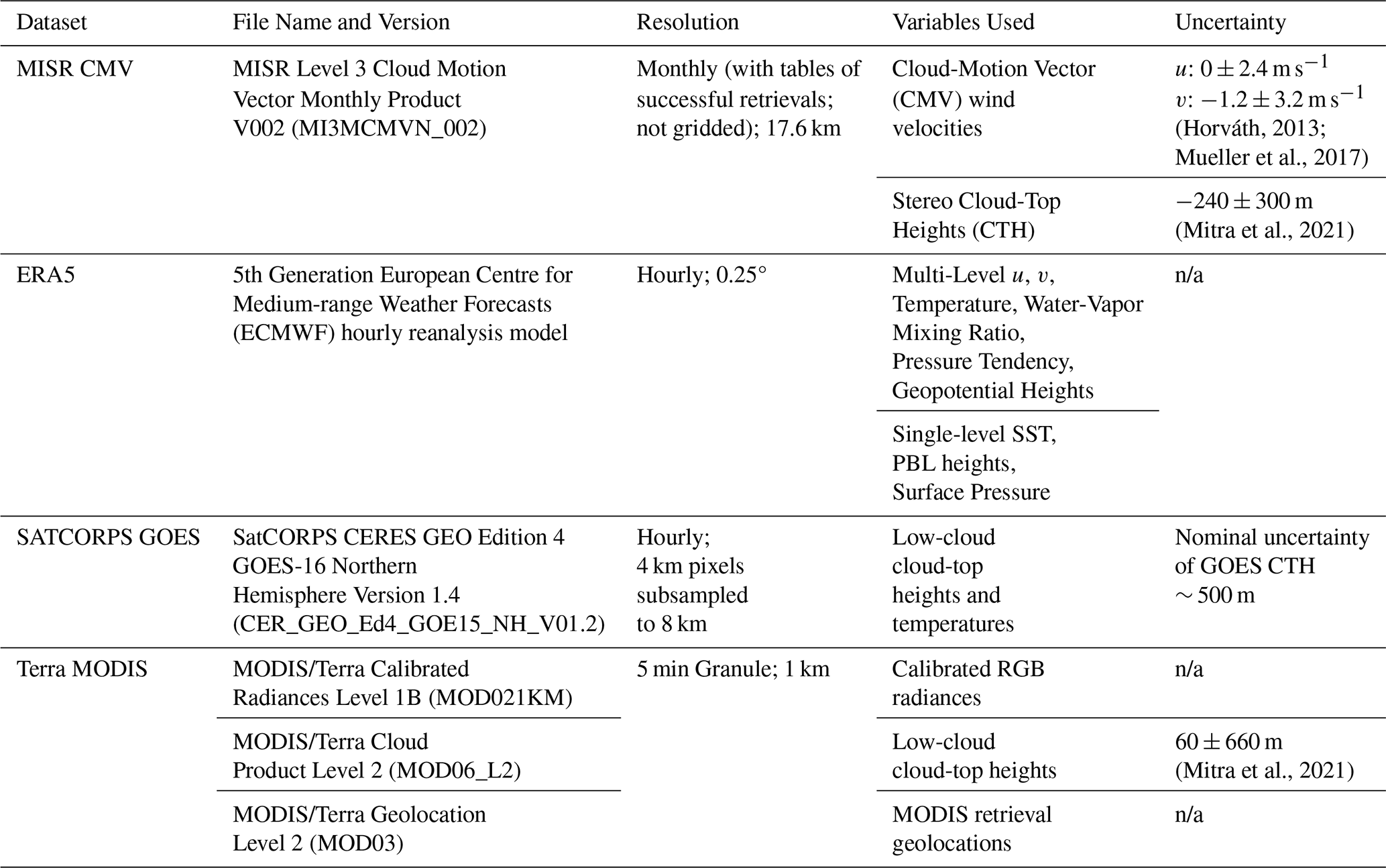
n/a: not applicable.

2.2.1 MISR Cloud Motion Vectors (CMVs)

The Multi-angle Imaging SpectroRadiometer (MISR) is a narrow-swath (∼ 380 km) multi-angular imaging instrument with nine cameras pointed at nadir and view angles of ±70.5°, ±60.0°, ±45.6°, ±26.1°, and 0 (nadir) (Diner et al., 1998). We use the MISR Level 3 CMV monthly product (Version F02_0002, MI3MCMVN_002), which provides stereoscopically derived cloud-top heights (CTHs) and collocated horizontal winds (u, v) at ∼ 17.6 km resolution. Although MISR also provides higher-resolution CTH retrievals at 1.1 km, here we use CTHs at the same resolution as the motion vectors for consistency.

Cloud-motion vectors are derived by tracking features across MISR's multi-angle imagery. Triplets of cameras with asymmetric view geometry are used to disentangle apparent motion due to parallax from actual horizontal motion, enabling simultaneous retrieval of wind and height (Moroney et al., 2002; Horváth, 2013). This retrieval is purely geometric and does not depend on ancillary thermodynamic profiles. As a result, MISR retrievals of cloud-top heights and winds have been demonstrated to be highly accurate and precise. A near-global comparison of MISR cloud-top heights against a space lidar revealed a bias ± precision of −240 ± 300 m for low clouds (Mitra et al., 2021). Meanwhile, depending on the method of validation, the zonal wind speed (u) was found to be nearly unbiased whereas the meridional wind speed (v) was shown to have a bias between −0.3 to −1.5 m s⁻¹, with precision typically in the range 2.4–3.7 m s⁻¹ (Horváth, 2013; Mueller et al., 2017). For this study, we shall use a nominal bias ± precision of 0 ± 2.4 m s⁻¹ for u and −1.2 ± 3.2 m s⁻¹ for v. Leveraging the well-characterized nature of the error characteristics, Mitra et al. (2021) closed the error budget for MISR cloud-top heights and motion-vector retrievals. As a result, we can propagate the known errors in MISR CMVs and CTHs to estimate retrieval errors in our retrievals of w and w_e.

Unlike many monthly satellite products, MISR CMVs are not pre-gridded but stored as lists of individual retrievals, tagged by time, geolocation, and orbit. This allows use at the single-overpass level. Here, we subset one descending-node daytime overpass intersecting the stratocumulus deck off California (4 June 2018). Standard quality screening is applied (QA > 50 or high-confidence retrievals only), and we retain only low clouds (CTH < 3 km) so that CMVs represent PBL-top winds.

2.2.2 ERA5 Reanalysis

The European Centre for Medium-range Weather Forecasts (ECMWF) reanalysis (ERA5; Hersbach et al., 2020) provides reference meteorological fields. Specifically, the profiles of horizontal winds (u, v), vertical pressure tendency (ω, Pa s⁻¹), temperature, geopotential heights and water vapor mixing ratio along with surface air pressure, sea-surface temperature and boundary layer height (BLH) are utilized. We have utilized the standard BLH available from the ERA5 archive rather than deriving it from various thermodynamic properties as done by von Engeln and Teixeira (2013) and acknowledge that the ERA5 BLH can differ significantly from the real values. We discuss the implications of this choice in Sect. 4. The pressure levels were converted to geometric height using the geopotential heights for direct comparison with MISR heights.

ERA5 vertical pressure tendency is converted to mesoscale vertical air motion (w) following:

$$\begin{array}{}\text{(24)}& w=-\mathit{\omega }{\displaystyle \frac{R_{\mathrm{d}}{T}_{\mathrm{v}}}{pg}},\end{array}$$

where, T_v is the virtual temperature, R_d is universal gas constant for dry air and g is acceleration due to gravity. The ERA5 boundary-layer height (BLH) was used as a proxy for cloud top height.

2.2.3 GOES (SatCORPS)

To provide an independent geostationary constraint, we use hourly cloud-top height (CTH) and cloud-top temperature (CTT) from the NASA SatCORPS dataset, which adapts CERES Edition 4 retrievals for GOES platforms (Minnis et al., 2020). For this study, GOES-15 (GOES-West) retrievals closest in time to the MISR overpass are collocated to the MISR grid and compared against MISR CTHs.

2.2.4 MODIS Terra Level-2 (MOD06)

To add a second estimate of CTH from a polarorbiter, we use CTH estimates from the Moderate Resolution Infrared Spectroradiometer (MODIS; MOD06_L2), also onboard Terra. MODIS CTH for low clouds (CTH < 3 km) are always derived based on conversion of retrieved infrared cloud-top temperatures (Platnick et al., 2017). MODIS CTHs are also collocated to the MISR grid to compare against the MISR estimates of CTH.

Algorithmic Implementation. All datasets are mapped to a regular latitude–longitude grid spanning the MISR swath, with 0.2° spacing in both latitude and longitude. This corresponds to ∼ 22 km meridionally and ∼ 19–20 km zonally over the subtropical oceans that are the area of interest and is comparable to the native ∼ 17.6 km MISR sampling. H_T, u, and v from the native MISR grid are linearly interpolated onto this mesh with grid cells lying farther than 0.2° from the nearest MISR retrieval left undefined to avoid extrapolation into data gaps.

Spatial derivatives are computed in metric space using great-circle distances. For each target grid cell (blue circle in Fig. 1), we gather all valid retrieval pairs that straddle the cell in the north–south direction and, separately, in the east–west direction within the analysis window appropriate to the diagnostic. For each pair, we calculate a slope as the difference in the field values divided by the great-circle separation along the meridional (N–S) or the zonal (E–W) directions, and the directional gradient is calculated as the arithmetic mean of these pairwise slopes. This extreme-pair approach is robust to swath gaps and returns $\frac{\partial \left(\cdot \right)}{\partial x}$ and $\frac{\partial \left(\cdot \right)}{\partial y}$ in native units per kilometre and the derivatives are undefined where the required neighbour pairs are absent.

Two window sizes are used (Fig. 1).

For divergence, a half-width of 0.4° stabilizes $\frac{\partial u}{\partial x}$ and $\frac{\partial v}{\partial y}$ and yields a reliable ∇_hV_h for Eq. (4). For the height-advection term $u\frac{\partial H_{\mathrm{T}}}{\partial x}+v\frac{\partial H_{\mathrm{T}}}{\partial y}$, a half-width of 0.2° preserves mesoscale structure in H_T. Units are kept consistent (either convert H_T to metres or the gradients to metres⁻¹), so that the final w and w_e retrievals are in m s⁻¹, which are finally reported in units of cm s⁻¹.

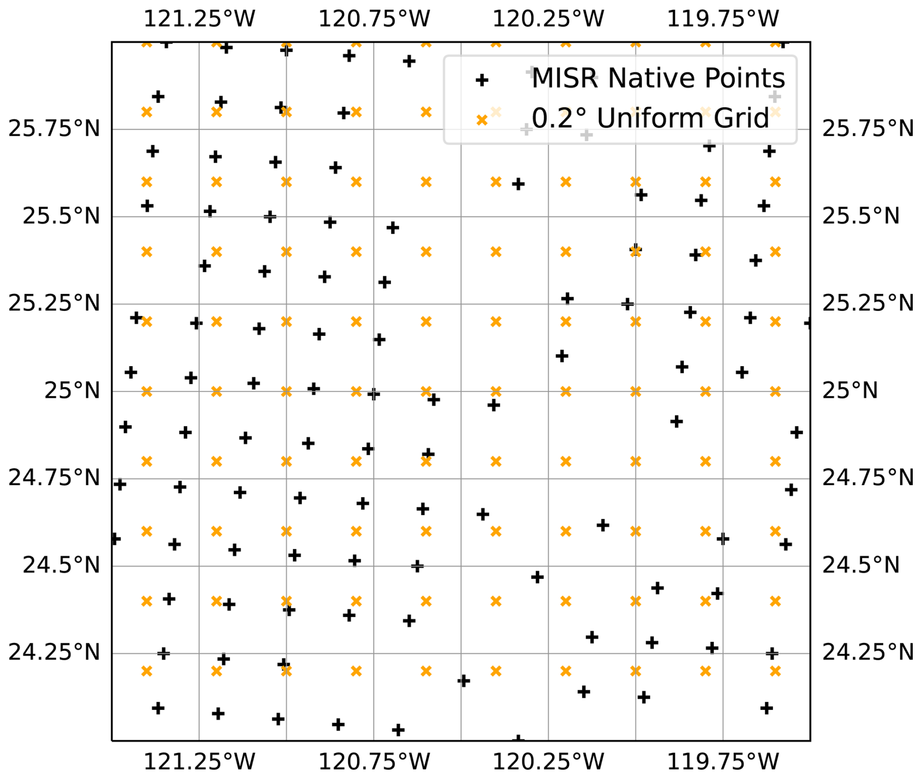
Figure 1 A zoomed-in view of the spatial distribution of the native MISR data grid (black plus signs) and the grid centres of the uniform 0.2° grid to which all MISR data is resampled (orange crosses). Also shown are the windows used to calculate derivatives for the estimation of vertical air velocity (dashed red) and entrainment rate (dashed black) at cloud-top for a target grid-cell (blue circle).

Because a single MISR overpass (which provides the snapshot from which our retrievals are made) can result in small-scale variability in w, the entrainment calculation replaces the pointwise w in Eq. (1) by a local environmental mean,

$$\begin{array}{}\text{(25)}& \langle w{\rangle }_{\mathit{\rho }}(x,y)={\displaystyle \frac{\mathrm{1}}{N_{\mathit{\rho }}\left(x,y\right)}}\sum _{d\le \mathit{\rho }}w\left(x^{\prime },y^{\prime }\right),\end{array}$$

where the average is taken over all valid neighbours within a radius ρ = 0.4° (great-circle metric). The operational entrainment used for this case is therefore derived from Eq. (5) as

$$\begin{array}{}\text{(26)}& w_{\mathrm{e}}(x,y)=u{\displaystyle \frac{\partial H_{\mathrm{T}}}{\partial x}}+v{\displaystyle \frac{\partial H_{\mathrm{T}}}{\partial y}}-\langle w{\rangle }_{\mathit{\rho }}(x,y)\end{array}$$

All outputs ($\frac{\partial u}{\partial x}$, $\frac{\partial v}{\partial y}$, $\frac{\partial H}{\partial x}$, $\frac{\partial H}{\partial y}$, w, w_e and the advective term $u\frac{\partial H_{\mathrm{T}}}{\partial x}+v\frac{\partial H_{\mathrm{T}}}{\partial y}$) are produced on the regular 0.2° mesh to which all input data had been resampled; grid cells lacking sufficient neighbors for the directional pairs or the local average remain undefined.

3 Results

We compare MISR wind vectors with collocated ERA5 fields and MISR CTH with independent CTH estimates from GOES–SatCORPS and MODIS, as well as ERA5 BLH. We then present MISR-derived w and w_e, evaluate them against equivalent diagnostics from ERA5, and quantify retrieval uncertainties. Intercomparisons of input variables are conducted at the native MISR CMV resolution (∼ 17.6 km), while derived fields are produced on the uniform 0.2°-resolution grid.

3.1 Case Description and Intercomparison

We analyse a single Terra overpass on 4 June 2018 sampling an unbroken marine stratocumulus deck off the California coast. All datasets (MISR CMV, ERA5, GOES–SatCORPS, MODIS) are restricted to this day and collocated to the MISR footprint. MISR retrievals are filtered to QA > 50 (high confidence retrievals only) and CTH < 3 km.

Figure 2a shows continuous low cloud with embedded cellular texture in GOES visible reflectance. MISR stereo CTH estimates were available for the whole sector, with few gaps due to cloud clearing and presence of cirrus clouds. As MISR reports the CTH above mean sea level, some of the cloud top heights could be negative. In fact, the acceptable values of MISR CTH in the operational MISR cloud-top height retrievals are −500 m to 20 km above mean sea level (with negative heights signifying cloud-top height retrievals below mean sea-level). Only 8 negative CTH values were present within this scene (all between −100 m to 0) and hence were neglected in further analysis. However negative CTH will need to be converted to heights over the geoid for retrieval calculations in further iterations of this implementation. The CTH increased from North to the South, with East-West changes being both positive and negative. The co-located MISR CMVs (Fig. 2b) depict a coherent North-westerly flow with gentle but organized gradients at the CMV resolution. The winds were north-westerly on the western end of the swath, and westerly on the eastern end North of 27.5° N. To the South of 27.5° N, the winds were north-westerly on the western end of the swath, and almost northerly at the eastern edge. This wind patterns and cloud top height changes are consistent with the higher-pressure system and high low-level cloudiness as over the Northeast Pacific as reported by Wood and Bretherton (2004). ERA5 boundary-layer heights (BLH) and winds for the overpass time (Fig. 2c) present a broadly consistent flow and a slowly varying inversion depth along the swath. However, around 30° N and −118.5° W, the ERA5 winds were north-westerly, as opposed to the MISR winds that were almost westerly. Moreover, ERA5 estimates of BLH are noted to be higher and less spatially variable when compared to MISR CTH.

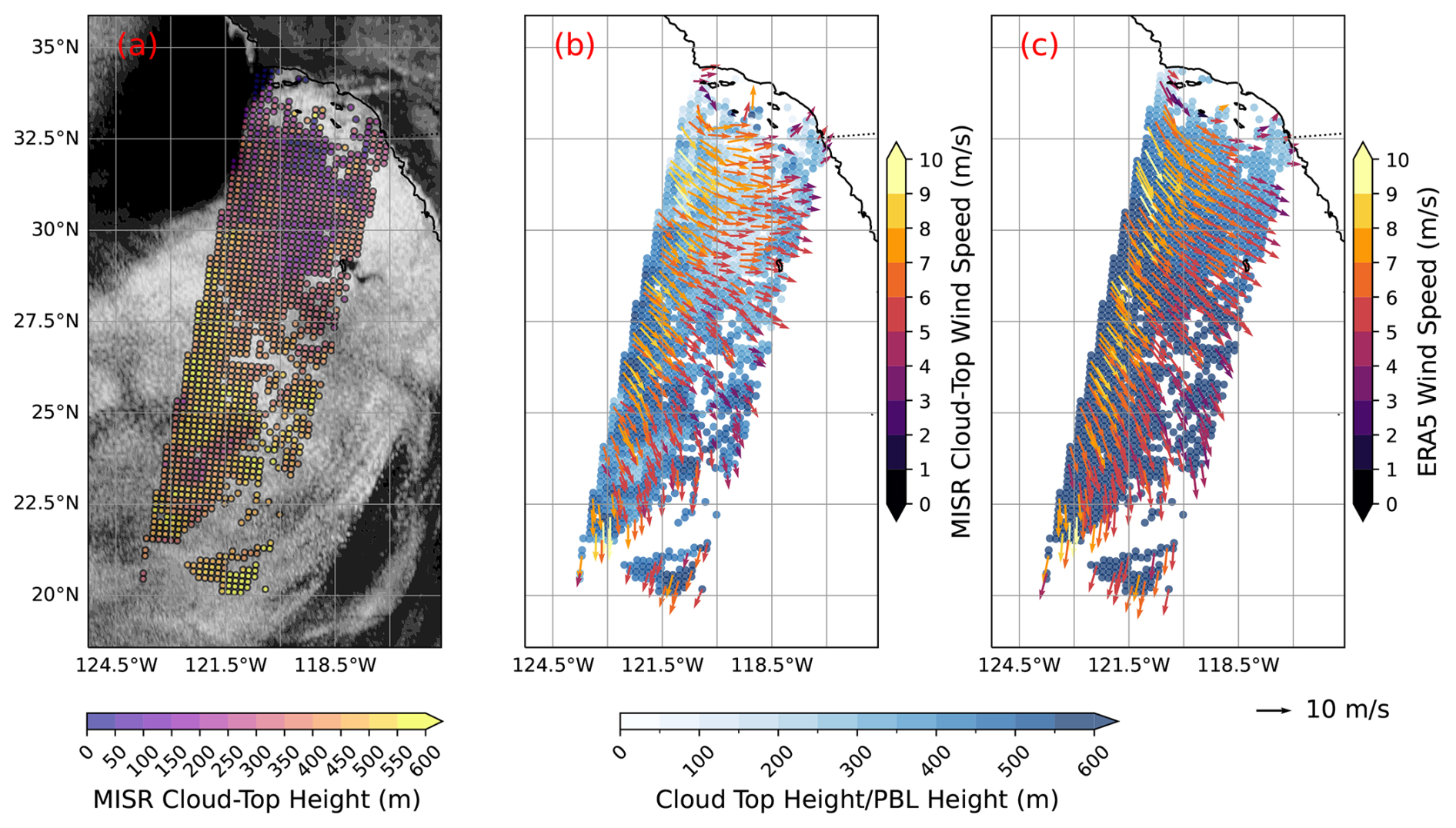
Figure 2 (a) GOES visible channel reflectance (greyscale) and MISR CTH for low clouds (colours), (b) MISR CTH (blue-scale colours) and MISR cloud-motion vectors (red scaled coloured arrows) and (c) ERA5 PBL depths (blue-scale colours) and ERA5 horizontal wind vectors (red scaled coloured arrows).

The MODIS visible satellite imagery shows similar patterns as GOES, showcasing widespread stratus coverage over the region (Fig. 3a). Due to higher spatial resolution, the cellularity of marine stratocumulus clouds is nicely visible in the MODIS imagery. Thin upper-level clouds are present near the coast as reported by the MODIS cloud top heights (Fig. 3b). Also visible are rectangular patches in the MODIS low cloud top height estimates. These are related to empirical adjustments made over discrete 1° latitude–longitude regions while converting MODIS retrieved low cloud-top temperatures to corresponding cloud-top heights (elaborated further while discussing Fig. 4).

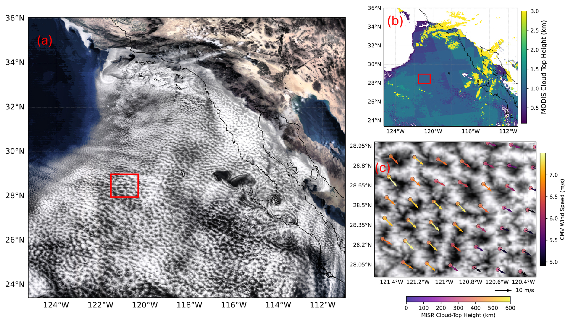
Figure 3 (a) MODIS True colour RGB imagery, (b) MODIS Cloud-top heights and (c) MODIS visible imagery over a small subset over the case study area with inlaid MISR cloud-top heights (coloured circles) and cloud-motion vectors (coloured arrows). In panels (a) and (b), the subset region shown in panel (c) is highlighted with a red box. To aid interpretation, panels (a) and (b) have been contrast-enhanced using luminance-based stretching and local equalisation to highlight the mesoscale cellular structures in the cloud field.

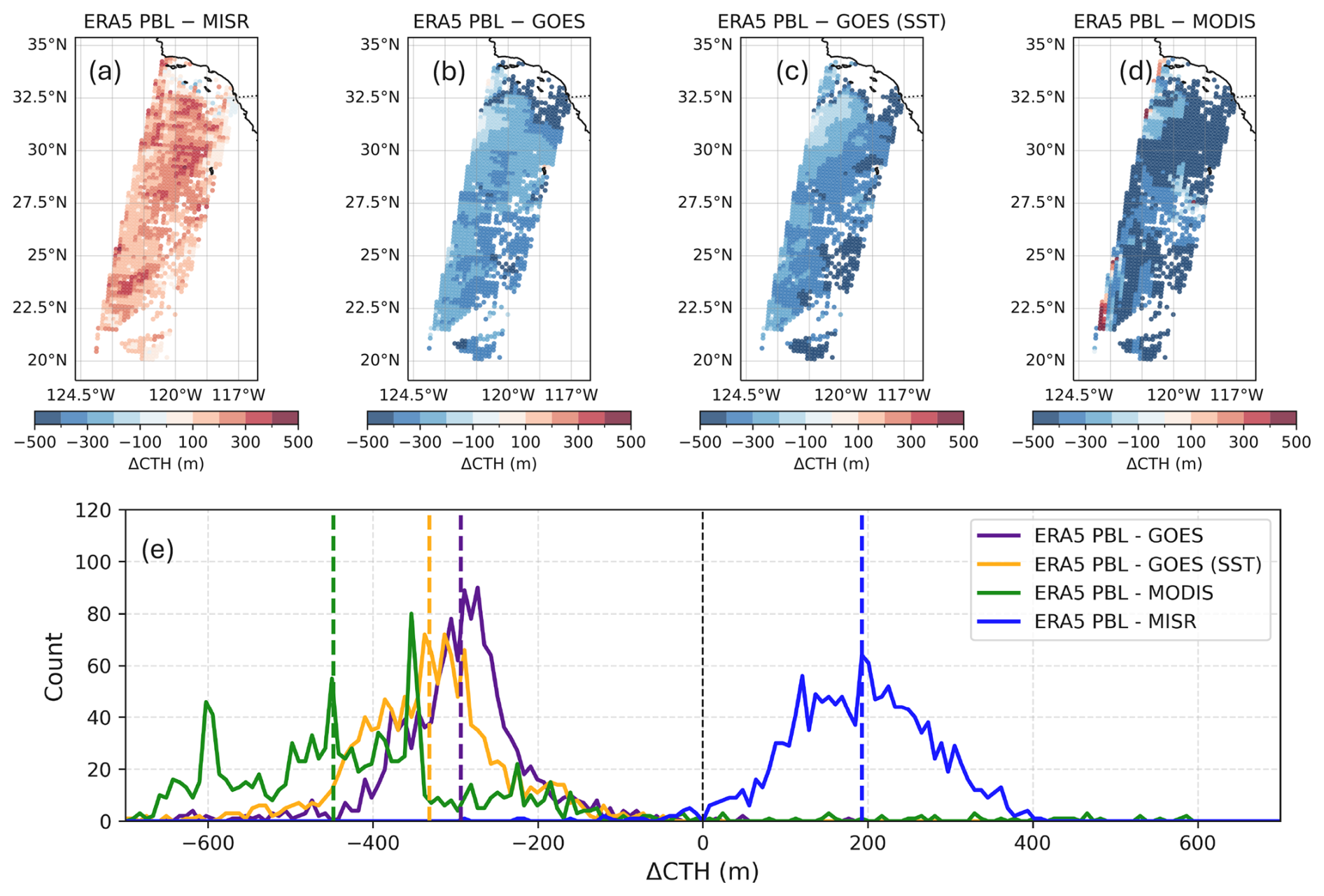
Figure 4 Differences between (a) ERA5 PBL depths and MISR CTH, (b) ERA5 PBL depths and GOES CTH, (c) ERA5 PBL depths and GOES-SST CTH and (d) ERA5 PBL depths and MODIS CTH. (e) Histograms of the differences between ERA5 PBL depths with MISR CTH (blue), GOES CTH (purple), GOES (SST) CTH (orange) and MODIS CTH (green). Mean differences for each histogram are depicted as dashed vertical lines of the corresponding colour.

In multilayer cloud scenes (e.g. cirrus over stratus), MISR's geometric stereo retrieves the lower cloud properties when the overlying cirrus is optically thin. Comparisons against space-borne lidar has shown a robust low-cloud detection by MISR for cirrus optical depth τ ≲ 0.3–0.4 (Mitra et al., 2021). Moreover, whenever the low cloud is detected, the accuracy of the retrieved low-cloud's CTH is not degraded by the thin cirrus above (Mitra et al., 2021, 2023). Conversely, for thicker cirrus τ > 0.5, MISR stereo retrieves cirrus top heights instead, and hence can be neglected from further low cloud analysis. This clear distinction in low versus high cloud retrievals of CTH within the MISR record is a distinct advantage over infrared techniques employed in other satellite sensors (GOES, MODIS), which often results in spurious “mid-level” cloud-height retrievals for multi-layered scenes. The data points that are not plotted along the MISR track plots in Fig. 1a are due to a mix of such cirrus contamination or low MISR CMV QA values.

Zooming into a subset of the field of MISR CTH and CMV wind vector retrievals against the backdrop of MODIS true colour imagery (Fig. 3c), individual cellular elements of the cloud structure can be visually resolved. MISR vectors delineate confluence around cell edges, i.e., the spatial structure that makes entrainment diagnosis meaningful at ∼ 17.6 km. Over this 1° × 1° region, wind speed changes of ∼ 2 m s⁻¹, and cloud top height changes of ∼ 300 m occurred. This further reinforces the ability of MISR CMV to capture the mesoscale variability in cloud and dynamical properties of marine stratocumulus decks.

Accurate cloud-top height (CTH) is a primary requirement for our retrieval framework. Figure 4 compares MISR CTH with independent estimates from GOES–SatCORPS and MODIS, and with the ERA5 boundary-layer height (BLH). We also include an empirical CTH derived from GOES cloud-top temperature (CTT) and ERA5 sea-surface temperature (SST) using the regression of Zuidema et al. (2009):

$$\begin{array}{}\text{(27)}& \text{CTH}={\displaystyle \frac{\text{SST}-\text{CTT}+\mathrm{1.35}}{\mathrm{0.0095}}}\end{array}$$

This relationship was developed over southeast Pacific stratocumulus to mitigate errors introduced by lapse-rate assumptions when converting CTT to height; as such, it is regionally tuned and may not generalize to all regimes.

Mean differences (ERA5 PBLH − CTH) over the domain are +188.9 ± 87.3 m (MISR), −343.2 ± 282.2 m (GOES), −359.2 ± 199.2 m (GOES-SST) and −608.2 ± 1037.0 m (MODIS). The signs and spreads are consistent with the expected behaviour of the retrievals. Thermal-infrared methods (GOES, MODIS) infer height from brightness temperatures using ancillary profiles that may not capture sharp, shallow inversions; when the inversion is strong, the radiances constrain cloud-top temperature poorly and heights tend to be biased high. Their errors also depend on low-cloud optical depth and temperature contrast, yielding broad distributions even within a single MISR scene (Mitra et al., 2021). MODIS operational adjustments based on climatological lapse rates reduce long-term biases but do not guarantee scene-specific accuracy, which is consistent with the larger spread and the 1° × 1° block-like discontinuities evident in Fig. 3b. Similar to MODIS, GOES CTHs exceed ERA5 BLH and MISR CTH; applying the GOES–SST regression further increases the overestimate in this case, suggesting that factors beyond SST (e.g., departures from a well-mixed boundary layer or regional tuning of the coefficients) contribute to the mismatch. By contrast, MISR uses geometric stereo to triangulate feature heights. In marine stratocumulus the tracked features often sit slightly below the radiative top, so MISR CTH is typically below the inversion, yielding a small positive BLH − CTH. Critically, this offset varies far less with optical depth than in IR methods (Mitra et al., 2021; Loveridge and Di Girolamo, 2025), producing a tighter distribution that is preferable when propagating height errors into the retrieval uncertainties of the divergence-based w and entrainment estimates (Sect. 2.1).

We compare MISR CMV winds with ERA5 at two levels: (i) the ERA5 pressure level closest to the MISR CTH and (ii) the ERA5 boundary-layer height (BLH). Figure 5 summarizes the differences. Sampling ERA5 at MISR CTH yields domain-mean (±1σ) differences of Δu = +0.01 ± 0.75 m s⁻¹, Δv = +2.17 ± 1.19 m s⁻¹ and Δ|V| = −1.42 ± 1.11 m s⁻¹ (MISR–ERA5). Sampling at ERA5 PBLH reduces the MISR–ERA5 speed bias to −1.17 ± 1.20 m s⁻¹, while leaving the components similar (Δu = +0.09 ± 0.77 m s⁻¹, Δv = +2.12 ± 1.24 m s⁻¹). The ∼ 0.25 m s⁻¹ improvement in speed bias is expected because height-assignment error projects onto winds through vertical shear. The first-order decomposition of wind-speed errors between two independent datasets can be written as:

$$\begin{array}{}\text{(28)}& \begin{array}{rl}\mathrm{\Delta }V& =\stackrel{\mathrm{height}\mathrm{assignment}}{\overbrace{\left({\displaystyle \frac{\partial V}{\partial z}}\right)\mathrm{\Delta }z}}+\stackrel{\mathrm{temporal}\mathrm{mismatch}}{\overbrace{\left({\displaystyle \frac{\partial V}{\partial t}}\right)\mathrm{\Delta }t}}\\ & +\stackrel{\mathrm{spatial}/\mathrm{scale}\mathrm{mismatch}}{\overbrace{V_{\mathrm{rep}}}}+\stackrel{\mathrm{retrieval}\mathrm{\&}\mathrm{collocation}}{\overbrace{{\mathit{\epsilon }}_{\mathrm{alg}}}},\end{array}\end{array}$$

where Δz is the mean offset between the true inversion height and level at which winds are retrieved. Moving from MISR CTH to ERA5 PBLH reduces Δz (Fig. 3), so the shear term $\left(\partial V/\partial z\right)\mathrm{\Delta }z$ shrinks and the speed bias decreases accordingly. That height-to-wind mapping is well-established as height assignment is often the dominant AMV error source and projects into vector differences through vertical shear (e.g., Velden and Bedka, 2009; Salonen et al., 2015; Córdoba et al., 2017).

The component asymmetry in this case, near-zero mean Δu but a persistent positive Δv of about 2 m s⁻¹ reflects MISR's viewing geometry and error anisotropy. On Terra's descending node, the along-track direction is approximately meridional, so the MISR v wind component maps closely to along-track motion, while u is predominantly cross-track. MISR's CMV algorithm derives motion from fore–nadir–aft image triplets separated by ∼ 3.5 min. The component errors are known to be larger in the along-track than the cross-track direction and to covary with stereo height errors because the same parallax geometry underpins both (Horváth, 2013). Residual geo-registration and co-registration artefacts can further introduce small, direction-dependent biases (e.g., noted in MISR–Meteosat intercomparisons; Lonitz and Horváth, 2011). These retrieval-intrinsic effects add to temporal offsets and representativeness differences, for example MISR provides instantaneous ∼ 17.6 km wind vectors at cloud top, whereas ERA5 wind estimates are an hourly ∼ 31 km analysis (e.g., Janjić et al., 2018). Together, these terms explain why the speed bias improves when sampling ERA5 at PBLH, yet the meridional component difference remains the dominant residual.

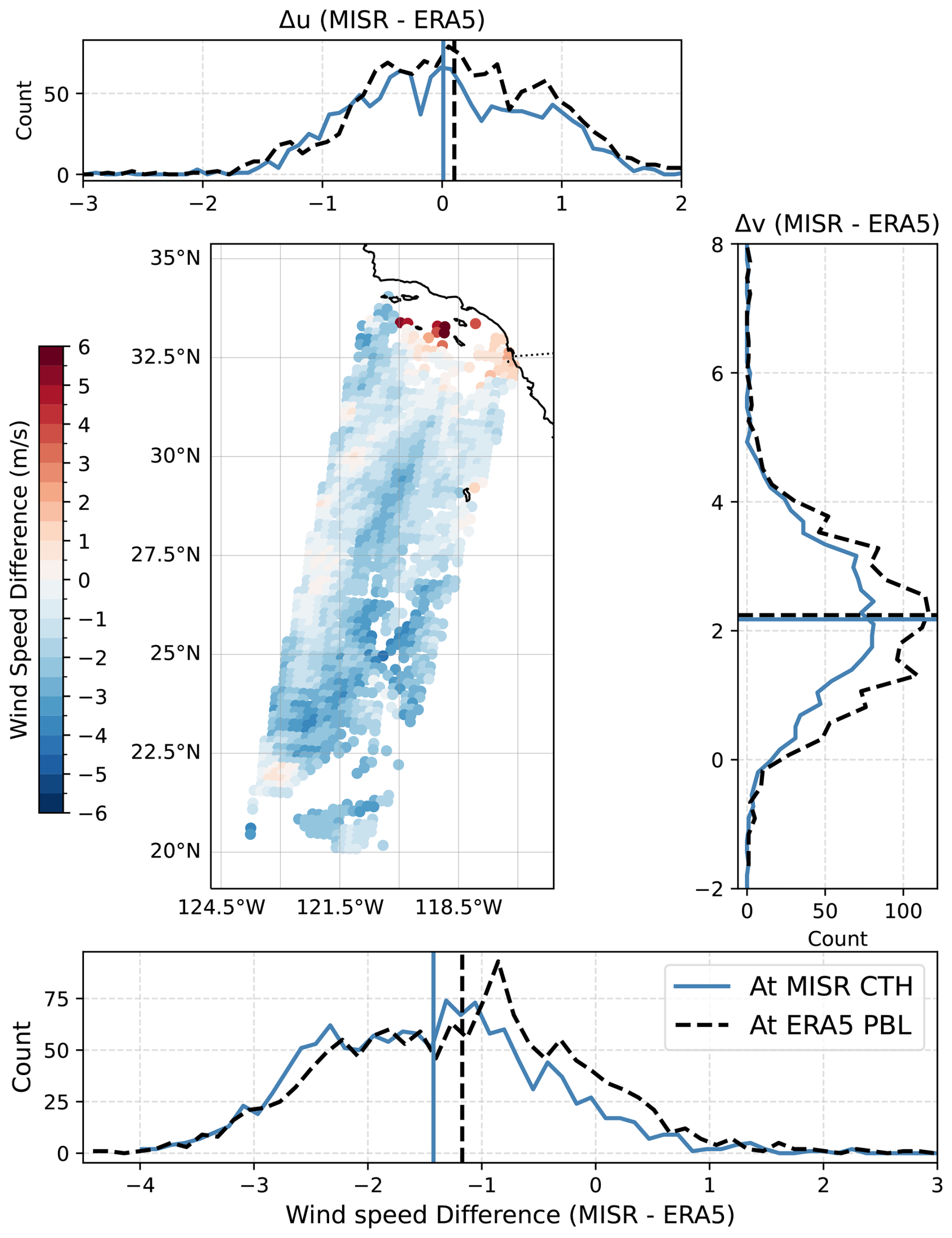
Figure 5 (a) Differences between MISR and ERA5 wind speeds at MISR CTH. Histograms of the differences between MISR and ERA5 (b) u-component of wind velocity, (c) v-component of wind velocity and (d) wind speeds at MISR CTH (blue) and at ERA5 PBL top (dashed black). For the histograms in panels (b), (c) and (d), all units are m s⁻¹ and the mean differences are denoted by vertical lines with the same style and colour of the corresponding histograms.

Crucially, this interpretation does not require invoking a global calibration error in MISR vectors. Rather, the data are consistent with (i) a small height-assignment contribution that diminishes when the comparison level better matches the inversion, (ii) anisotropic along-track uncertainties intrinsic to the stereo-tracking geometry, and (iii) temporal and spatial scale mismatches between an instantaneous stereo observation and an hourly coarser reanalysis data.

In summary, the 4 June 2018 scene is a low-topped, cellular stratocumulus deck in which MISR stereo cloud top heights and winds resolve mesoscale strain and confluence at ∼ 20 km scales, enabling stable wind divergence and entrainment retrievals.

3.2 Retrievals

We retrieve mesoscale cloud-top vertical air velocity (w) and mesoscale cloud-top entrainment rates (w_e) using both MISR CMV u and v at MISR CTH and for ERA5 u and v at ERA5 BLH, for the 4 June 2018 scene (Sect. 2.2.1; Eqs. 4 and 6). All such input parameters were re-gridded to, and the retrievals are output on a common and uniform 0.2° grid. During the retrievals, the height-advection term ($u\frac{\partial H}{\partial x}+v\frac{\partial H}{\partial y}$) is also output for comparative analysis against the retrieved w and w_e. Figure 6 summarizes the cloud-top vertical velocity w, the entrainment velocity w_e, and the height-advection term for MISR, ERA5, and their differences (MISR-ERA5). The portion of the swath shown originally comprised of 1397 MISR data points, out of which w and w_e retrieval was made for 1312 (∼ 94 %) and 1336 (∼ 96 %) points, respectively. The differences in the number of valid retrievals is due to the different window sizes used to calculate their underlying derivatives (Fig. 1).

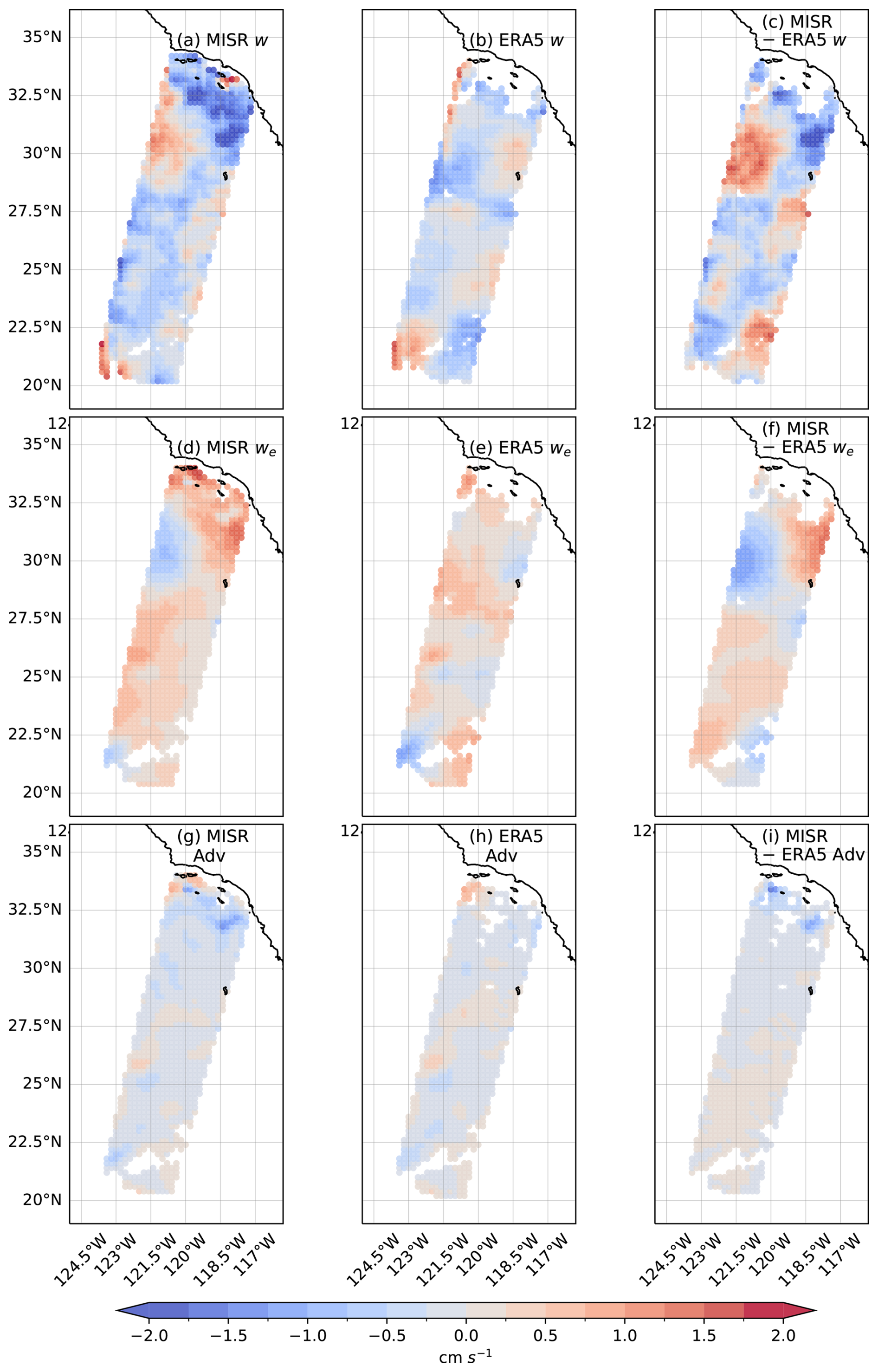
Figure 6 (a) MISR w retrievals (b) ERA5 w (c) Differences between MISR and ERA5 w (d) MISR w_e retrievals (e) ERA5 w_e (f) Differences between MISR and ERA5 w_e (g) MISR CTH advective term (e) ERA5 PBL height advective term (f) Differences between MISR and ERA5 PBL advective terms.

MISR w (Fig. 6a) exhibits a clear meridional dipole near the coast with intricate mesoscale structure at the same resolution as the retrieval (∼ 0.2°). There is markedly stronger descent near the coast, followed by a region of ascent centred around 30° N, followed by a region of weaker descent dotted with patches of very weak ascent. The domain mean and standard deviation are −0.36 ± 0.65 cm s⁻¹. Meanwhile, ERA5 w (Fig. 6b) shows a broadly similar large-scale pattern but is smoother in its features and extents of ascent-descent regions. The domain mean and standard deviation are −0.22 ± 0.45 cm s⁻¹. The difference of MISR and ERA5 w (Fig. 6c) is largely of the same pattern as that of MISR w (Fig. 6a). This is likely because MISR retrievals of CTH carry more spatial structure than does the corresponding field of ERA5 PBL heights (Fig. 2b and c), which resolves cell-scale convergence/divergence that the smoother underlying fields of ERA5 filters. The domain mean and standard deviation of differences in ERA5 and MISR derived mesoscale vertical air motion at the cloud top is 0.14 ± 0.73 cm s⁻¹.

MISR w_e (Fig. 6d) is predominantly positive across the deck with a gentle NE-SW gradient; the domain mean and standard deviation are 0.28 ± 0.40 cm s⁻¹. Meanwhile ERA5 w_e (Fig. 6d) is also predominantly positive with a domain mean and standard deviation are 0.19 ± 0.33 cm s⁻¹. Since the ERA5 retrieved w near the coast is not as negative as that from MISR, ERA5 retrieved w_e near the coast is not as positive as that from MISR. Moreover, the locations of negative values of MISR and ERA5 w_e are dissimilar in places. However, their MISR-ERA5 w_e differences (Fig. 6e) are typically low at such locations, and the differences are likely much lower than random uncertainties associated with these retrievals. The domain mean and standard deviation of ERA5 and MISR cloud-top entrainment rates is −0.09 ± 0.46 cm s⁻¹ (also, Fig. 7b).

The advection term A ($u\frac{\partial H_{\mathrm{T}}}{\partial x}+v\frac{\partial H_{\mathrm{T}}}{\partial y}$) is weak in both products (Fig. 6g–h) and its difference is near zero over most of the scene (Fig. 6i), with a domain statistic of −0.09 ± 0.19 cm s⁻¹. Thus, for this case, differences in the retrieved advective component contributes little to the MISR-ERA5 mismatch in w_e, which is largely driven by the differences in retrieved values of w. Which, in turn, reflects the greater spatial heterogeneity in MISR CTH relative to ERA5 BLH. From Eq. (8), w_e = A−w (positive w upward). Therefore, for samples with upward mesoscale vertical motion (w > 0), obtaining positive entrainment requires the height-advection term to exceed the upward motion. When A is small, positive w_e tends to occur where w is weakly negative (subsiding).

The retrievals for this case compare well with those from the previous studies. The domain mean and standard deviation of mesoscale vertical air motion was −0.36 ± 0.65 cm s⁻¹, which is much weaker than the 50 hPa h⁻¹ (11.7 cm s⁻¹) reported by Bony and Stevens (2019) in the tropics. The domain mean and standard deviation of entrainment velocity was 0.28 ± 0.40 cm s⁻¹. This estimate is in the ball-park of the estimates reported by Painemal et al. (2017) of −0.4 to 0.8 cm s⁻¹ in the South Atlantic, 0.723 cm s⁻¹ reported by Ghate et al. (2019) in the North Pacific, 0.57 cm s⁻¹ by Faloona et al. (2005) in the coastal California, 0–0.5 cm s⁻¹ as reported by Caldwell et al. (2005) in the South Pacific. As expected, the MISR entrainment velocity estimates for the stratocumulus case analyzed herein are much weaker than the 0–20 cm s⁻¹ entrainment velocities reported by Tornow et al. (2023) for a cold-air outbreak case. The MISR estimates were also within the range of 0–1 cm s⁻¹ entrainment velocities reported by Albrecht et al. (2016) for a continental stratocumulus case. It should be noted that due to MISR's overpass at 10:30 LT, the derived entrainment rates are likely at the lower end given the strong diurnal cycles reported by Painemal et al. (2017) and Caldwell et al. (2005). The GOES derived entrainment rates by Painemal et al. (2017) for the southeast Atlantic Stratocumulus deck were negative between 07:00 and 13:00 LT, which partly explains the negative values of MISR entrainment rates as they are made at 10:30 LT.

As a further sanity check of the retrieved values, we compared MISR-derived entrainment rates against independent estimates obtained using GOES cloud-top heights and winds following the mass-budget framework of Painemal et al. (2017). In this approach, GOES–SST cloud-top heights (Fig. 4) are combined with ERA5 horizontal wind fields sampled at the GOES–SST cloud-top heights to estimate cloud-top vertical velocity and entrainment rates using the same continuity and mass-budget formulation described in Sect. 2.2.1. Over the analysis domain, GOES-derived entrainment velocities ($w_{\mathrm{e}}^{\mathrm{GOES}}$) exhibit the same sign and mesoscale spatial coherence as the MISR-derived values, indicating consistent diagnosis of entraining versus detraining regions across the cloud deck. However, the domain-mean $w_{\mathrm{e}}^{\mathrm{GOES}}$ (0.44 ± 0.35 cm s⁻¹), is larger than the corresponding MISR ($w_{\mathrm{e}}^{\mathrm{MISR}}$) mean, yielding a mean difference ($w_{\mathrm{e}}^{\mathrm{MISR}}-w_{\mathrm{e}}^{\mathrm{GOES}}$) of −0.28 ± 0.35 cm s⁻¹. This amplitude offset is not unexpected, given the reliance of the GOES-based estimate on infrared cloud-top height retrievals and reanalysis winds, both of which tend to smooth cloud-top gradients and can project height-assignment differences into the diagnosed divergence and vertical motion. In contrast, the height-advection term (A) derived from GOES remains weak, with a domain mean of 0.05 ± 0.38 cm s⁻¹, similar to the MISR-based estimate and close to zero across most of the scene. Thus, while the magnitude of $w_{\mathrm{e}}^{\mathrm{GOES}}$ differs from $w_{\mathrm{e}}^{\mathrm{MISR}}$, the qualitative behavior and spatial organization of entrainment are robust across independent satellite frameworks.

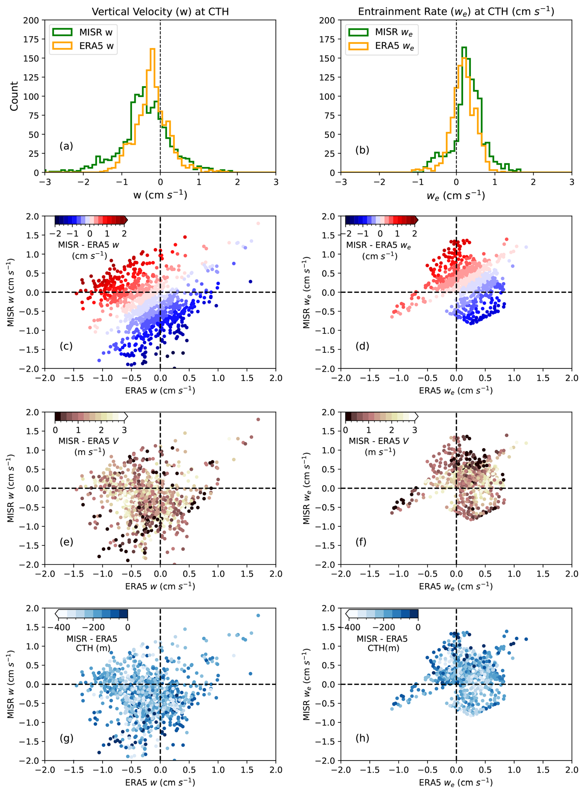
Figure 7 (a) Histograms of MISR (green), ERA5 (orange) and differences in MISR and ERA5 (purple) w (b) Histograms of MISR (green), ERA5 (orange) and differences in MISR and ERA5 (purple) w_e (c) Differences of MISR and ERA5 w as a joint distribution of ERA5 and MISR w (d) Differences of MISR and ERA5 w_e as a joint distribution of ERA5 and MISR w_e (e) Differences of MISR and ERA5 wind speeds at ERA5 PBL heights (V) as a joint distribution of ERA5 and MISR w (f) Differences of MISR and ERA5 wind speeds at ERA5 PBL heights (V) as a joint distribution of ERA5 and MISR w_e (g) Differences of MISR CTH and ERA5 PBL heights as a joint distribution of ERA5 and MISR w (h) Differences of MISR CTH and ERA5 PBL heights as a joint distribution of ERA5 and MISR w_e.

The statistics of the overall distributions of the ERA5 and MISR derived w and w_e for the case are depicted in Fig. 7. We quantify similarity between the ERA5 and MISR histograms by the area of overlap between their respective normalized probability densities (0–1 with 1 identical). The distribution of ERA5 and MISR w (Fig. 7a) for the case was largely similar (79 % overlap), with the MISR reported w having a longer negative tail (stronger subsidence). The percentage of retrievals of descent (negative w) is slightly greater in MISR (982; 75 %) than ERA5 (959; 73 %). Overall, the percentage of retrievals with descent stronger than 2 cm s⁻¹ (i.e., w < −2 cm s⁻¹) is 13 % in MISR and 3 % in ERA5. Moreover, the distribution of ERA5 and MISR w_e (Fig. 7b) for the case was largely similar (81 % overlap), with the MISR derived w_e having a longer positive tail (stronger cloud-top entrainment). The percentage of retrievals with valid cloud-top entrainment or positive w_e is greater in MISR (950; 71 %) than ERA5 (867; 65 %). Overall, the percentage of retrievals with cloud-top entrainment stronger than 0.5 cm s⁻¹ (i.e., w_e > 0.5 cm s⁻¹) is 28 % in MISR and 17 % in ERA5.

While visually, one may detect the presence of a general linear co-variability between ERA5 and MISR retrievals of w and w_e (Fig. 7c and d), there are enough high sample-level differences that result in poor correlation between the two pairs of retrievals. The coefficient of linear correlation between MISR and ERA5 w is 0.2 and between MISR and ERA5 w_e is 0.25. Differences between ERA5 and MISR w are found to lie within ±0.25 cm s⁻¹ for ∼ 25 % of all retrievals, while differences between ERA5 and MISR w_e are found to lie within ±0.25 cm s⁻¹ for ∼ 32 % of all retrievals.

Figure 7e, f, g, h show that there is no strong systematic relationship between the point differences in the input parameters (i.e., wind speeds and cloud-top heights) and the differences in the retrievals from ERA5 and MISR. This suggests that the point differences in retrieved estimates of w and w_e from MISR and ERA5 likely depend strongly on the spatial patterns in the 2D field of the input parameters and not the underlying point estimates of the input parameters.

An interesting subset of points (N = 32) in these figures are the samples for which MISR-ERA5 cloud-top wind speed differences are negative and absolute CTH differences are less than 50 m (darker colours in the bottom left quadrant of Fig. 7e and g and in the top right corners of Fig. 7f and h). Unlike these points, MISR estimates of CTHs and winds are typically lower than respective ERA5 estimates (Figs. 4 and 5). The mean difference in MISR and ERA5 CTHs for these points are 51 ± 58 m and the mean difference in MISR and ERA5 wind speeds at CTH are −2.1 ± 2.4 m s⁻¹. The majority (25 out of 32) of these points result in negative w and positive w_e retrievals from both MISR and ERA5. For these points, the mean difference between MISR and ERA5 retrievals of w is −0.5 ± 0.5 cm s⁻¹ and the mean difference between MISR and ERA5 retrievals of w_e is −0.25 ± 0.33 cm s⁻¹. Thus, close agreement in pointwise cloud-top height does not eliminate the systematic wind-speed difference; it persists (and can even increase) because part of the MISR wind-component uncertainty is directionally anisotropic (along-track vs cross-track) and does not vanish with improved height co-location (see Sect. 3.1).

With scene-mean input uncertainties σ_u = 2.4 m s⁻¹, σ_v = 3.2 m s⁻¹ and σ_H = 300 m (and the windowed derivatives described in Sect. 2.1), random uncertainties for each retrieval point are propagated using Eqs. (10)–(13) and systematic uncertainties are propagated using Eqs. (17)–(19). Mean propagated systemic uncertainty in w and w_e (i.e., Δ_w, ${\mathrm{\Delta }}_{w_{\mathrm{e}}}$) are found to be −0.6 cm s⁻¹ and −0.4 cm⁻¹ respectively. The mean random uncertainty in w and w_e (i.e., σ_w, ${\mathit{\sigma }}_{w_{\mathrm{e}}}$) are found to be 0.7 and 0.5 cm s⁻¹, respectively. Fractional uncertainties (${\mathit{\sigma }}_w/\mathrm{|}w\mathrm{|}$) are calculated from these estimates of random uncertainty and their relationship with the underlying CTH is studied in Fig. 8. As expected, for very low values of cloud-top vertical velocity and entrainment velocities (w, w_e ∼ 0), the fractional uncertainty can be asymptotically large.

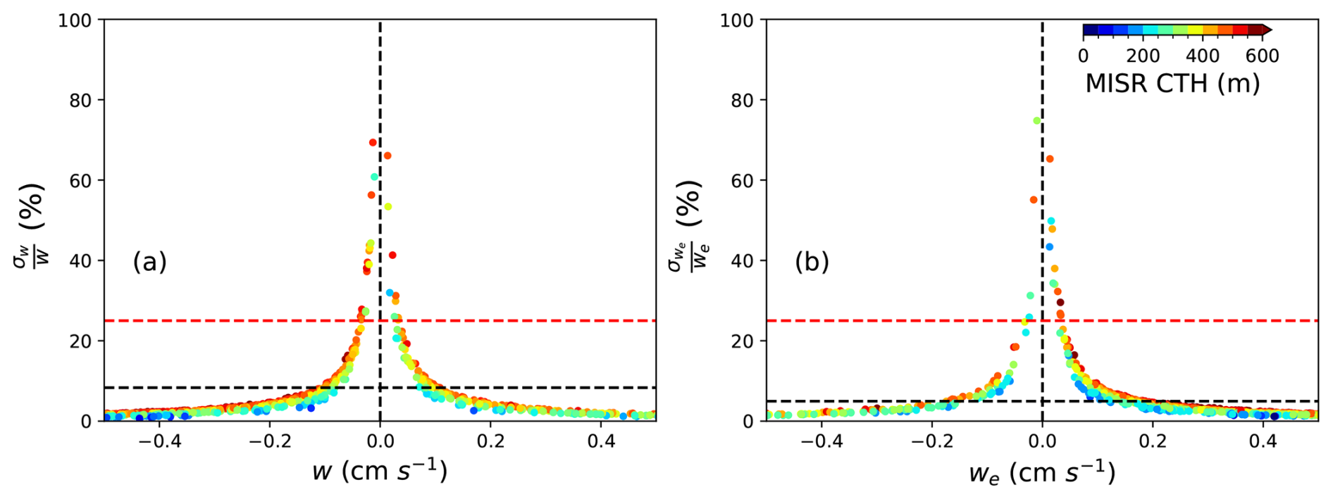
Figure 8 (a) Pointwise fractional uncertainty of MISR-based retrievals of w (i.e., ${\mathit{\sigma }}_w/\mathrm{|}w\mathrm{|}$) against the retrieved w. (b) Pointwise fractional uncertainty of MISR-based retrievals of w_e (i.e., ${\mathit{\sigma }}_{w_{\mathrm{e}}}/\mathrm{|}{w}_{\mathrm{e}}\mathrm{|}$) against the retrieved w_e. For both panels, black dashed lines show the domain-mean fractional uncertainties; red dashed lines mark a 25 % benchmark. The sharp rise near w, w_e ∼ 0 reflects division by small magnitudes.

Based on visual examination of the distributions of fractional uncertainty (Fig. 8), an ad hoc threshold of 25 % fractional uncertainty is chosen for “physically meaningful” retrievals. For the present scene, fractional uncertainties lower than the 25 % threshold are found for 1268 (i.e., 97 %) points for w retrievals and in 1122 (i.e., 85 %) points for w_e retrievals. Mean fractional uncertainty over all points are calculated to be 11 % for w retrievals and 5 % for w_e retrievals.

As noted in Sect. 2.2.1, the estimates of σ_w, ${\mathit{\sigma }}_{w_{\mathrm{e}}}$ are merely retrieval uncertainties, which scale with successive independent sampling. For the scene considered, using typical mesoscale lengths from the literature (e.g., L_x = L_y = 40 km; Wood and Hartmann, 2006), the correlation area is estimated as A_c ≈ π × 40 × 40 km ≈ 5000 km². The analyzed domain in our study covers an area approximately 2.0 × 10⁵ km², hence, N_eff; space ≈ 40, and the sampling standard errors for scene-means (from Eq. 25) are

$$\begin{array}{rl}& {\text{SE}}_{\mathrm{sampling}}\left(\stackrel{\mathrm{‾}}{w}\right)\approx {\displaystyle \frac{\mathrm{0.7}}{\sqrt{\mathrm{40}}}}=\mathrm{0.11}\mathrm{cm}{\mathrm{s}}^{-\mathrm{1}};\\ & {\text{SE}}_{\mathrm{sampling}}\left(\stackrel{\mathrm{‾}}{w_{\mathrm{e}}}\right)\approx {\displaystyle \frac{\mathrm{0.5}}{\sqrt{\mathrm{40}}}}=\mathrm{0.08}\mathrm{cm}{\mathrm{s}}^{-\mathrm{1}}\end{array}$$

These numbers are merely representative and are subject to change for actual values of A, L_x, L_y. As more scenes are aggregated within a homogeneous regime (e.g., same region/season and similar synoptic background), the random component of the mean retrieval uncertainty narrows roughly by a factor of $\mathrm{1}/\sqrt{N_{\mathrm{eff}}}$. A suitable averaging strategy to improve sampling precision for future atmospheric process-based analyses can focus on regime-based aggregation of multiple overpasses from the same season and synoptic class (e.g., similar lower-tropospheric stability, SST, and PBL depth).

However, it should also be noted that the scaling of random errors with $\mathrm{1}/\sqrt{N_{\mathrm{eff}}}$ does not happen indefinitely. This is because systematic contributors to the MISR precision budgets – such as uncertainties arising from discrete pixel registration or along-track anisotropy in retrieved wind components – do not average down and can only be treated by instrument-level calibration or explicit algorithmic improvements. Estimating this irreducible component robustly requires an independent reference (e.g., aircraft or surface-based observations) across multiple independent scenes within a given weather regime.

4 Summary and discussions

Entrainment of warm, dry air from above the cloud layer into the cloud is a critical process that modulates microphysical and radiative properties and, in turn, cloud lifetime (Wood, 2012; Bretherton et al., 2007; Mellado, 2017). Here we show that cloud-top vertical velocity w and entrainment velocity w_e can be retrieved from MISR alone using stereoscopic cloud-top height H_T and cloud-motion vectors (u, v). Because MISR provides co-located heights and winds at ∼ 17–18 km resolution, the retrieval operates at mesoscale, i.e., the scale at which stratocumulus organization increasingly appears to control longevity and transitions (Vogel et al., 2022). The approach is physically grounded: we diagnose w from continuity and w_e from a boundary-layer mass budget using only MISR inputs, with no reliance on reanalysis vertical motion or ancillary thermodynamic profiles. As a result, systematic and random uncertainties can be traced directly to the well-characterized MISR errors in height and wind (Horváth, 2013; Mueller et al., 2017; Mitra et al., 2021; Loveridge and Di Girolamo, 2025).

Applied to a stratocumulus deck off the United States West Coast on 4 June 2018, MISR and ERA5 give the same qualitative picture: weak descent on average and predominantly positive entrainment. MISR-retrieved w and w_e compare well against those from the ERA5 for this case (especially in central statistics), despite the differences in the temporal and spatial resolutions. MISR retains mesoscale structure in H_T and winds that the comparatively smoother reanalysis field cannot. Hence, divergence – and thus, w – differs in detail even when the scene mean agrees. Known anisotropy of the MISR along-track component also projects into the divergence (Horváth, 2013; Lonitz and Horváth, 2011).

Previous satellite retrievals of cloud-top entrainment typically utilized cloud-top height estimates from infrared sensors but estimates of vertical motion in those approaches were typically taken from a reanalysis into a mass budget consideration (e.g., Painemal et al., 2017; Zhu et al., 2025a, b). Despite the overall coverage and benefits of such retrievals, the most influential term, i.e., vertical motion (w_e) is not an observational estimate. Rather, it is taken from a model, so the largest and least traceable uncertainty in the retrieval method sits outside the observations. Our approach differs from those efforts by keeping the calculation strictly grounded within the observations. Here, both height and wind estimates come from the same stereo geometry, and both carry tight validation. For low clouds, MISR heights are accurate to a few hundred metres and winds to a few metres per second, with biases that are small and stable (Horváth, 2013; Mitra et al., 2021). Those properties allow us to propagate uncertainties through to w and w_e at each grid point. In the case examined, typical random uncertainties are about 0.7 cm s⁻¹ for w and 0.5 cm s⁻¹ for w_e; even screening for fractional uncertainties less than 25 % retains upwards of 85 % of all retrievals. These features make the retrieval suitable for both case studies and climatological aggregation (Vallejos et al., 2014).

While this study demonstrates the feasibility of retrieving cloud-top vertical velocity and entrainment rates from MISR observations alone, it does not constitute a formal validation of the retrieved magnitudes. The comparison with ERA5 serves only as a physical consistency check and contextual reference. A rigorous evaluation would require independent observations of vertical motion, inversion height, and entrainment at comparable spatial scales. Long-term ground-based facilities such as the ARM Eastern North Atlantic (ENA) site provide a promising opportunity in this regard, combining frequent radiosondes with cloud radar and Doppler lidar observations in marine stratocumulus regimes. A future evaluation strategy could involve regime-based compositing of MISR overpasses collocated with ENA observations and statistical comparison with entrainment estimates derived from mixed-layer budgets or turbulence diagnostics. Such an approach would respect inherent spatial and temporal mismatches while providing an independent test of the MISR retrieval framework.

Cloud-motion vectors are an underused bridge between cloud physics and dynamics. Recent work has shown that the MISR CMV record can reveal circulation changes on decadal scales, underscoring the benefits of analysing these vectors at their native resolution and with care for their error budgets (Di Girolamo et al., 2025). The present study takes a complementary step: using those same CMVs at low cloud-top to observe entrainment directly, with uncertainties that are explicit and portable. As Terra satellite has been in a very stable orbit from 2000–2023 yielding CTH and CMV estimates accurate enough for trend characterization, an operational data-product based on proposed retrieval technique is straightforward to envision. For each MISR overpass, inputs would be interpolated to a 0.2° grid and processed as in Sect. 2 (potentially complemented by standard spatial smoothing techniques) to deliver gradients, divergence, the height-advection term, and the derived w and w_e. Each grid cell would carry propagated random and systematic uncertainties and simple quality flags (e.g., a fractional-uncertainty mask, neighbour counts for gradients, thin-cirrus indicators). Monthly aggregates on a coarser grid would support climatology.

The scientific use cases of such a product can be varied. Process modellers can compare instantaneous retrievals of w and w_e with large-eddy simulation (LES) or single-column model output for the same scenes to test entrainment parameterizations and mixing assumptions (Bretherton et al., 2007; Mellado, 2017; Wood, 2012). Climatologists can build a 2000–2023 record of w and w_e for low clouds by region and season, characterize decadal changes and trends, and explore how entrainment covaries with stability, surface forcing, and aerosol sensitivity (Nam et al., 2012; Vial et al., 2013; Grosvenor et al., 2018; Xu et al., 2022; Luo et al., 2020). One can use the overall record to target days and regions for in-depth study with complementary data from Atmospheric Radiation Measurement (ARM) observatories and field campaigns, where Doppler radars, lidars, and surface instruments can provide independent checks on vertical motion and discontinuities at the inversion level (Albrecht et al., 2016; Shupe et al., 2012; Borque et al., 2016).

Appendix A

The retrieval technique (Sect. 2.2.1) makes few assumptions, and we explore their validity here. The mesoscale vertical air motion is derived from the continuity equation applied to the MISR CMV reported wind vectors (Eq. 4). The derivation assumes that the gradients in the horizontal winds at the cloud top are the same throughout the PBL, and the mesoscale vertical air motion is zero at the surface. The profiles of gradient in horizontal winds ($\frac{\partial u}{\partial x}$, $\frac{\partial v}{\partial y}$) derived from the ERA5 data for the case (Fig. A1a) shows that the values are uniform throughout much of the boundary layer (expressed in normalized units ξ = $z/\text{PBL Height}$, where z is height above the surface). The ERA5 w profile (derived from ERA5 reported pressure tendency through hydrostatic conversion) varies only weakly with height over the same extent of the ERA5 reported PBL depth. This region is dominated by gentle subsidence with mean vertical air motion at the surface and CTH differing only by a small amount (surface: −0.05 ± 0.54 cm s⁻¹; CTH: −0.35 ± 0.74 cm s⁻¹).

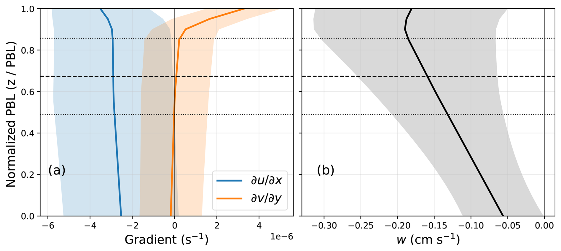
Figure A1 ERA5 mean profiles on a normalized PBL coordinate ($z/\text{BLH}$) (a) Horizontal wind-gradient components $\frac{\partial u}{\partial x}$ (blue) and $\frac{\partial v}{\partial y}$ (orange); (b) vertical velocity w (black) (positive upward). Solid curves show the mean and shaded envelopes denote one standard deviation variability. Horizontal dashed lines show mean (thick) and standard deviation (thin) of MISR retrieved heights (transformed to the normalized PBL coordinate).

As noted in Fig. 4, MISR CTH are lower than ERA5 PBL depths on average by 189 ± 87 m, over the region considered. Thus, MISR CTHs are found to lie on average at ξ = 0.68 ± 0.18. Interestingly, Fig. A1a and b show that MISR-derived stereo CTHs are a better estimate than ERA5 reported PBL depths (i.e., ξ = 1) as the typical structure of a well-mixed boundary layer ($\frac{\partial u}{\partial x}$, $\frac{\partial v}{\partial y}$ uniform with height and a nearly linear profile of w) is found below MISR CTHs. In Fig. A2, we compare two independent ERA5 vertical air motion estimates at PBL top:

• i.

  a continuity estimate, w_c = $-H_{\mathrm{T}}\left(\frac{\partial u}{\partial x}+\frac{\partial v}{\partial y}\right)$ from ERA5 winds and PBL heights using Eq. (4)

• ii.

  a hydrostatic estimate, w_h, derived from ERA5 reported pressure tendencies.

The average difference between the two estimates was −0.15 ± 0.4 cm s⁻¹. There is a moderate correlation between the two estimates (r = 0.5) with the best-fit line showing a small offset of 0.18 cm s⁻¹. If the assumptions involved were completely self-consistent, we would see an exact 1:1 line. These deviations from that ideal scenario are likely due to implementation artefacts (e.g., finite-difference gradients on the native grid) and assumptions in deriving w_h (e.g., hydrostatic balance and ideal gas law with virtual temperature). Crucially however, the sign agreement between w_c and w_h and their near-linear co-variation show that the continuity estimate captures the same mesoscale signal at PBL top as the hydrostatic form to first order.

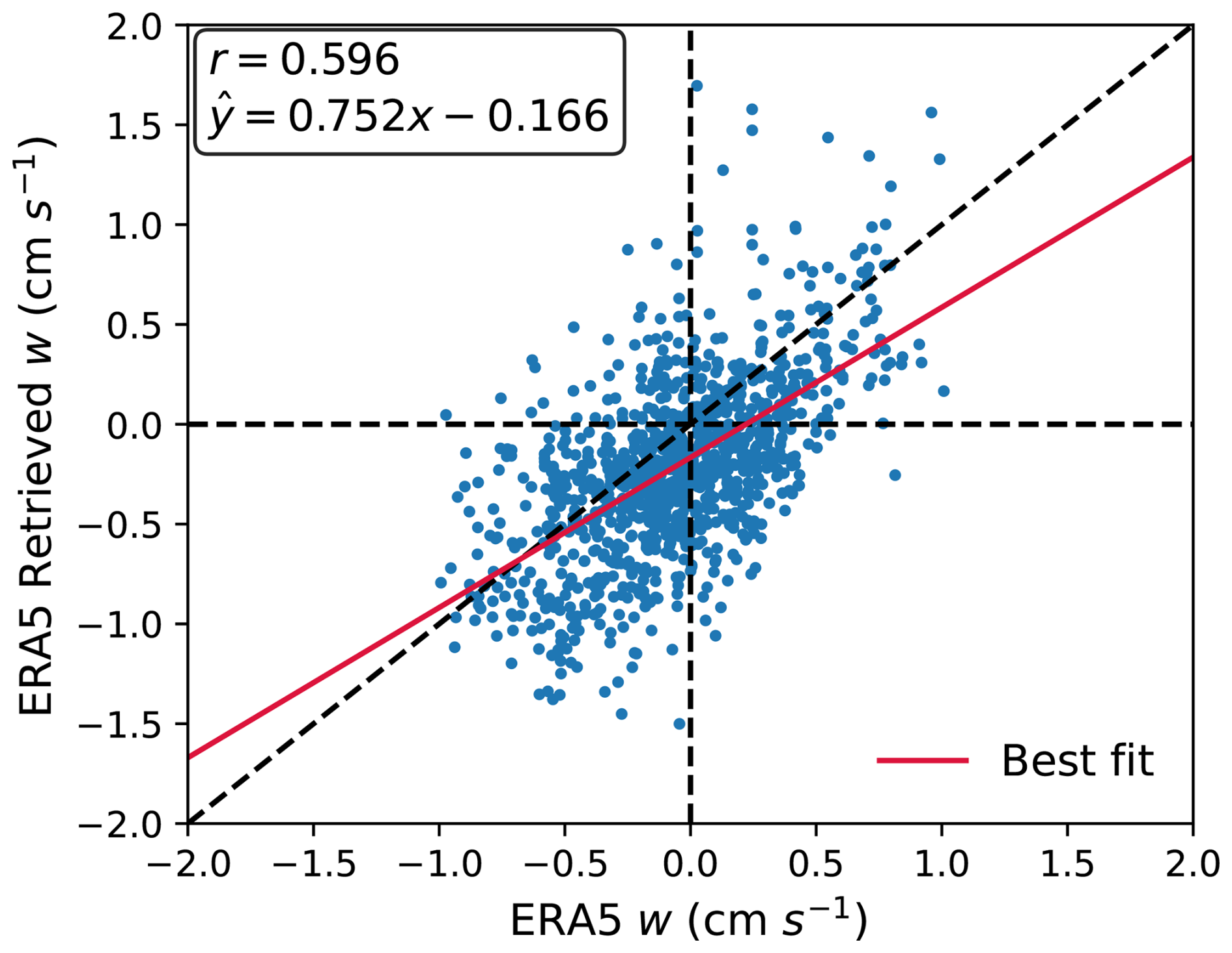
Figure A2 Scatter comparison of ERA5 vertical velocity at PBL top against the continuity-based ERA5 retrieval (from horizontal wind divergence). Each marker is a co-located grid cell. The dashed black line is the 1:1 line; the solid red line is the least-squares fit (equation shown). The upper-left inset reports the Pearson correlation coefficient (r).