Chemical sparsity in Bayesian receptor models for aerosol source apportionment

Aerosol source apportionment is a key tool for understanding the origins of atmospheric particulate matter and for guiding effective air quality management strategies. However, source apportionment techniques still struggle to properly separate highly correlated sources without relying on restrictive a priori information, possibly skewing the solution and adding subjective operator input, with varying degrees of benefit. This study introduces sparsity into the Bayesian Autocorrelated Matrix Factorisation (BAMF) model with the aim of removing non-essential species contribution in the unconstrained profiles, which is expected to improve the separation of factors compared to BAMF. The regularised horseshoe prior (HS) has been added to BAMF (BAMF+HS) to promote composition matrix F sparsity, shrinking low-signal contributions to the solutions. BAMF+HS was evaluated using three synthetic datasets designed to reflect increasing levels of data complexity (Toy, representing a highly simplified dataset; Offline, representing a filter dataset; and Online, representing an Aerosol Chemical Speciation Monitor (ACSM)-like dataset), and a real-world multi-site filter dataset. The results demonstrate that BAMF+HS effectively enforces sparsity in offline datasets and that this improves accuracy in reconstructing source profiles and time series compared to BAMF and Positive Matrix Factorisation (PMF). However, its application to higher-complexity ACSM datasets revealed sensitivity to sampling instability hindering sparsification. With that, even though sparsity was not achieved, the quality of the BAMF+HS solution metrics were not deprecated compared to BAMF. Overall, this work underscores the value of incorporating profile sparsity as a solution property in Bayesian source apportionment, and positions BAMF+HS as a promising model for source apportionment.

1 Introduction

Particulate Matter (PM) adversely affects human health through both short and sustained exposures (Pope and Dockerty, 1999; Yang et al., 2019). The observed relationship between decreasing PM concentrations and increased life expectancy (Keuken et al., 2013; Zheng et al., 2022) highlights the importance of developing mitigation plans grounded in detailed knowledge of PM sources composition and concentrations. Moreover, because some proxies for aerosol toxicity, among them oxidative potential, are highly dependent on its sources (Daellenbach et al., 2020), implementing source-specific mitigation measures contributes to more quantitative and efficient abatement and a more effective protection of the population.

Source apportionment is the process of identifying and quantifying sources by using information about their chemical composition, and is commonly conducted through receptor models (RMs) which differentiate PM sources according to the distinctness of their chemical composition and time series characteristics. The most widely used RM is the Positive Matrix Factorisation model (PMF, Paatero and Tapper, 1994), which deconvolutes the input chemical composition into the product of composition and time series matrices (F and G, respectively), and minimises the residuals of the fit through the weighted least squares loss. The factorisation equation, hence, is written as

$$\begin{array}{}\text{(1)}& \mathbf{X}=\mathbf{G}\cdot \mathbf{F}+\mathbf{E},\end{array}$$

where X is the input matrix, a n⋅m matrix of n timepoints and m species, which is decomposed into G and F, matrices of dimensions n⋅p and p⋅m, respectively, where p is the number of factors, and E is the residuals matrix of dimensions n⋅m.

Unconstrained PMF, although it can lead to robust results, is usually insufficient when the sources are highly correlated or have very similar source profiles. In such cases, guiding the model by introducing a priori knowledge (common practice known as constraining the model) has been proven beneficial for the source deconvolution (Lingwall and Christensen, 2007; Belis et al., 2019; Dinh et al., 2025). However, it can still introduce substantial bias in the solution (Via et al., 2022). Globally, the RMs cover the whole range of pollution sources knowledge required prior to receptor modelling (Viana et al., 2008; Belis et al., 2013). A very strongly-constrained RM is the Chemical Mass Balance model (CMB), which factorises the initial matrices with a totally fixed G or F.

Bayesian models represent a probabilistic alternative to the PMF framework. The first application of Bayesian models in atmospheric source apportionment was introduced in Park et al. (2001, 2002) for Volatile Organic Compounds (VOC) source apportionment. In this approach, the mass closure condition was taken to the Bayesian framework and an autocorrelation prior, AR(1) (the first order autoregression formulation), was applied, improving the solution given assuming independent G components. The autocorrelation prior importance was later reinforced in Rusanen et al. (2024) with a differently formulated autocorrelation prior. The latter shows the added value of the Bayesian Autocorrelated Matrix Factorisation model (BAMF) compared with PMF across different spectrometry-based PM synthetic datasets. The Bayesian Multivariate receptor modelling software BNFA and bayesMRM (Park et al., 2021) were developed to provide user-friendly tools for Bayesian source apportionment.

However, studies using the Bayesian Matrix Factorisation framework are still scarce. Some examples are Oh and Park (2022), which employed a Bayesian RM to conduct multi-site source apportionment, and Zhang et al. (2023), which performed NH${}_{\mathrm{4}}^{+}$ source apportionment through the Bayesian SIMMR package (Govan et al., 2023). Bayesian models have also been used as a complement to standard RMs, as in Balachandran et al. (2013) where a Bayesian model processing ensemble solutions of a chemical transport model and solutions of three RMs are produced to then use it in CMB for production of final results. The Bayesian model focused on attributing the proper weight to each of the ensemble components and improved the correlation of sources with their markers compared to the traditional approach. Bayesian inference has also been used in Park et al. (2002) and Dai et al. (2024) to generate spatially resolved source apportionment solutions adjusting the weights of each location solution in a multi-site data scheme.

Thus, Bayesian Matrix Factorisation has become an effective and powerful tool for aerosol source apportionment. However, to the authors knowledge, little attention has been given to improving the accuracy of chemical composition profiles, i.e. F components. This highlights the fundamental challenge in receptor modelling of obtaining chemically distinct and interpretable source profiles from complex and mixed emission sources. Moreover, it has been shown in Rusanen et al. (2024) that in BAMF, slight differences of F can severely compromise the quality of G (Fig. S2 in the mentioned article), hence, steps towards F refining should result in overall source apportionment method improvement. In this context, sparsity, defined as the property of a dataset, model or solution in which only a limited number of elements are substantial contributions while most are zero or close to zero, could be favourable for this problem. The accomplishment of sparse source fingerprints could represent “cleaner” emission sources with less mixing among resolved factor profiles, since substituting non-significant contributions in a factor by zeros might allow allocating more importance to the actually relevant contributions of species in factors. This work aims to implement sparsity on chemical fingerprints in BAMF aiming for a more accurate source apportionment. We introduce sparsity with the regularised horseshoe prior (Piironen and Vehtari, 2017), which unlike other sparsity priors, enables regularisation of the sparsity strength, and compare it with other sparsity priors, such as Lasso (Rasmussen and Bro, 2012) and Spike-and-slab (Andersen et al., 2014). This model is then tested on three synthetic datasets with different complexity degrees and one real-world dataset to depict the impact of sparsity and potential benefits of its implementation.

2 Methodology

2.1 Bayesian Matrix Factorisation

Bayesian Matrix factorisation models, like other RMs, are based on the chemical mass balance equation (Eq. 1). Bayesian modeling approaches this problem probabilistically and bases the determination of the matrices, F and G, the main parameters to determine, upon the assumptions imposed on the model, i.e. priors. Bayesian factorisation forces the decomposition through modelling the X matrix components as a Gaussian with center on the “noise-free data matrix” Z (matrix of dimensions n⋅m) and a standard deviation given by the positively-defined uncertainty matrix (Eq. 2). The matrix σ (positive matrix of dimensions n⋅m) represents the uncertainties of the measurements. The matrix Z is, in turn, the product of the time series and profiles submatrices, G and F, respectively, and (a) is rewritten as:

$$\begin{array}{}\text{(2)}& \mathbf{X}\sim N(Z,\mathit{\sigma })=N(\mathbf{G}\cdot \mathbf{F},\mathit{\sigma })\end{array}$$

where N represents the normal distribution. With that formulation, the measurements matrix X is modeled into a Gaussian distribution whose centre is the G⋅F product matrix and its standard deviation is the uncertainty matrix σ. In turn, one introduces certain restrictions on the F, G matrices characteristics in the form of priors. Whilst G is not given any prior and is sampled then by default from a uniform distribution, F is modelled as a Dirichlet distribution to ensure positivity, with the sum of its components being equal to 1 (Eq. 2):

$$\begin{array}{}\text{(3)}& {\mathbf{F}}_k\sim \mathrm{Dirichlet}\left({\mathrm{1}}_m\right)\end{array}$$

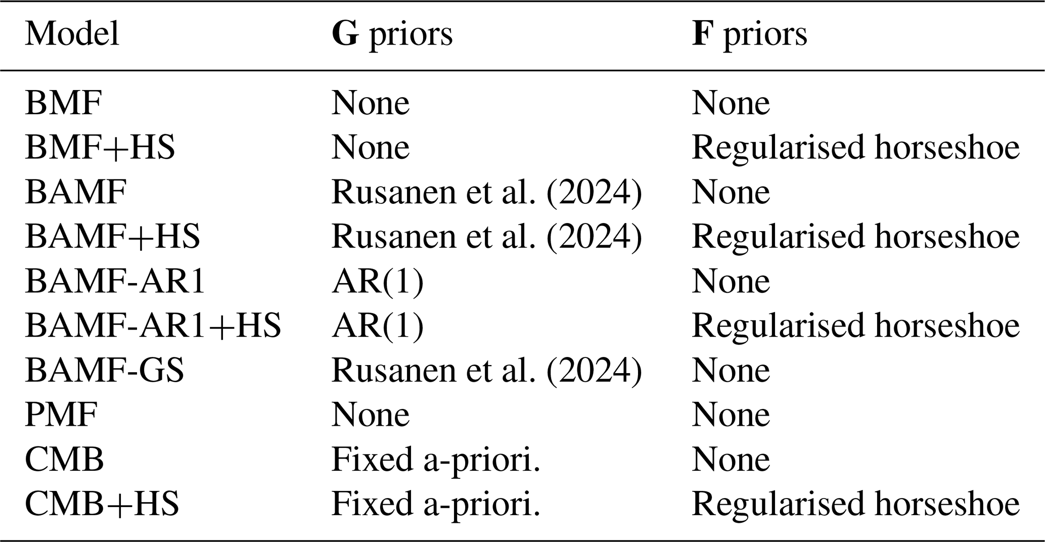
with these F requirements, profiles represent the normalised contribution to the spectra of one source. Usual notation for indices used hereinafter are i, j, k for elements in the range (1, …, n), (1, …, m), and (1, …, p), for the timestamps, species, and factors, respectively. It is worth noting that PMF applies the normalisation of profiles after a F, G solution is found, not as a model prior as done in BAMF. The PMF generates mass-loaded F, G solution matrices, which are reweighted to provide a normalised F and a mass-loaded G. In the Bayesian models used in this study, the normalisation of F is inherent to the model by design. The different formulations eventually provide normalised F and mass-weighted G, with unlikely affectations due to the normalisation procedure. The model configuration given by Eqs. (2) and (3) will be referred to as Bayesian Factorisation model (BMF) and represents the analog of PMF in the Bayesian framework. All models used in this manuscript are outlined in Table 1.

Table 1 Models used in the current study and their priors on the G, F matrices.

On top of this structure, Rusanen et al. (2024) proposed an autocorrelation prior for G which should account for the inherent autocorrelation of air pollutant sources in time. The imposition of autocorrelation in G entails that two consecutive measurements should be more similar than two measurements apart in time, and that the similarity should fade with the temporal gap between them. This property is particularly advantageous for atmospheric pollution dynamics which, generally, are expected to exhibit temporal smoothness rather than abrupt fluctuations. The formulation of the autocorrelation prior for G is given by Eq. (4) and includes two more modelling parameters, α (positive vector or dimension p) and β (positive vector or dimension p), which regulate the similarity of one G component with the previous one as follows:

$$\begin{array}{}\text{(4)}& {\mathbf{G}}_{i+\mathrm{1},k}\sim C^{+}({\mathbf{G}}_{ik},{\mathit{\alpha }}_k\cdot \mathrm{\Delta }{t}_i+{\mathit{\beta }}_k)\end{array}$$

where i∈ (2, …, n−1), represents the Cauchy distribution and ⁺ represents positive real numbers. This prior centers the i+1th component distribution in the ith component with a distribution width that linearly depends on the temporal gap between these two timestamps. Hence, the more temporally-separated two consecutive points are, the less correlated they are expected to be. The Cauchy distribution was chosen due to its heavier tails which enable more probable jumps between consecutive i^′s than a Gaussian distribution (Gelman et al., 2014). This flexibility could be convenient for real-world datasets which are affected by measurement gaps. The coefficients α and β are source-dependent to allow for source-dependent correlation degrees. The model which introduces this prior to BMF is called Bayesian Autocorrelated Matrix Factorisation model (BAMF, Rusanen et al., 2024).

2.1.1 The horseshoe prior

Here we propose a sparsity enforcement into the profiles matrix, intending to remove small contributions of irrelevant species for a given factor. The introduction of sparsity in BAMF involves the addition of several hyperpriors in the F prior to implement the shrinkage mechanism. In this study, we used the regularised horseshoe prior (Piironen and Vehtari, 2017), which is a global-local complex of hyperpriors, i.e. the shrinkage power is both regulated globally source-wise and F-component-wise. The idea behind this prior is that species with very small contributions to a factor are shrunk toward zero through an automatic shrinkage mechanism, whereas species with substantial support from the data are largely unaffected. The regularised horseshoe (HS) prior implemented in F in the BAMF scheme as

$$\begin{array}{}\text{(5)}& {\mathbf{F}}_{kj}={\mathit{\mu }}_{kj}\cdot {\stackrel{\mathrm{̃}}{\mathit{\lambda }}}_{kj}\cdot {\mathit{\tau }}_j,\end{array}$$

where μ (matrix of dimensions n⋅m) represents the F matrix without the horseshoe prior. μ, in turn is defined as a standard Cauchy distribution prior as

$$\begin{array}{}\text{(6)}& {\mathit{\mu }}_{kj}\sim C^{+}(\mathrm{0},\mathrm{1}),\end{array}$$

where τ (vector of dimension p) represents the global shrinkage parameters and

$$\begin{array}{}\text{(7)}& \mathit{\tau }\sim C^{+}(\mathrm{0},{\mathit{\tau }}_{\mathrm{0}}\cdot {\mathit{\sigma }}_{\mathrm{HS}}),\end{array}$$

where the parameter τ₀ can be regulated by the user to regulate the overall shrinkage power and σ_HS is sampled from an uniform distribution. The hyperparameter ${\stackrel{\mathrm{̃}}{\mathit{\lambda }}}_{kj}$ applies the local shrinkage to as

$$\begin{array}{}\text{(8)}& {\stackrel{\mathrm{̃}}{\mathit{\lambda }}}_{kj}=\sqrt{{\displaystyle \frac{c^{\mathrm{2}}\cdot {\mathit{\lambda }}^{\mathrm{2}}}{c^{\mathrm{2}}+{\mathit{\lambda }}^{\mathrm{2}}\cdot {\mathit{\tau }}^{\mathrm{2}}}}},\end{array}$$

where

$$\begin{array}{}\text{(9)}& {\displaystyle }{c}^{\mathrm{2}}\sim {\mathrm{\Gamma }}^{-\mathrm{1}}(\mathrm{0.5}\cdot \mathrm{slab}\mathit{\_}\mathrm{d}f,\mathrm{0.5}\cdot \mathrm{slab}\mathit{\_}\mathrm{d}f)\text{(10)}& {\displaystyle }\mathit{\lambda }\sim {\mathrm{slab}}_{\mathrm{scale}}\cdot C^{+}(\mathrm{0},\mathrm{1})\end{array}$$

both combined providing the characteristic shrinking horseshoe shape. Here, λ is a model parameter of dimensions n⋅m which after regularisation becomes is denoted as $\stackrel{\mathrm{̃}}{\mathit{\lambda }}$ Further description of the horseshoe implementation on BAMF can be found in Sect. S2 in the Supplement, and the prior derivation and details in Piironen and Vehtari (2017). The distribution parameters τ₀, σ_HS, and slab_df, slab_scale were tested and results did not show significant sensitivity to their variations, so we keep the default ones asprovided in Piironen and Vehtari (2017) in their available shared codes. The models with the horseshoe (HS) priors are hereinafter marked with “+HS”. Figure S1 in the Supplement shows a schematic diagram of the matrix decomposition through BAMF.

In order to assess the amount of sparsity of a dataset or a solution, we used the Gini coefficient (Gini, 1936), which assesses the inequality over a distribution as follows:

$$\begin{array}{}\text{(11)}& \mathrm{Gini}={\displaystyle \frac{{\sum }_{i=\mathrm{1}}^n(\mathrm{2}\cdot i-n-\mathrm{1})\cdot x_i}{\mathrm{2}\cdot n\cdot {\sum }_{i=\mathrm{1}}^n{x}_i}}\end{array}$$

where x values are sorted in ascending order, and n is the number of elements in x. It is a proxy for how deviant a dataset is from the total equality amongst its components. Since it quantifies the inequality, it can be a proxy for sparsity; if some values are high and the others are zero, Gini ≈1 (great inequality), if all values are equal, Gini =0. Also, the solution-to-truth Gini values ratio will be discussed throughout the analysis, referred to as “Gini ratio”. To evaluate if the sparsity is enforced precisely where it should, an additional metric has been applied called “zero truth sum”. This metric sums up the modelled contributions of the null species in the truth profiles.

2.1.2 Alternative factorisation methodologies

BAMF-AR1. There is an alternative formulation for the autocorrelation prior as introduced in Bayesian models by Park et al. (2001). The AR(1) autocorrelation prior is the first degree polynomial expansion of the autoregressive models and it proposes a linear progression of ${\mathit{G}}_{i+\mathrm{1},k}$ from G_i,k. We introduce AR(1) in the Bayesian framework as

$$\begin{array}{}\text{(12)}& {\mathit{G}}_{i+\mathrm{1},k}\sim N({\mathit{\alpha }}_k\cdot {\mathit{G}}_{ik}+{\mathit{\beta }}_k,{\mathit{\gamma }}_k)\end{array}$$

In this formulation, the i+1th point stems from a Gaussian distribution centered linear combination on the ith point with source-dependent slopes (α) and intercept (β), and width (γ). Although, unlike Eq. (4), it disregards the decrease of correlation between gapped consecutive points, this prior allows for source-specific time series trends, which would be beneficial for certain source description. The model which introduces this prior to BMF will be called BAMF-AR1.

BAMF-GS. Another formulation is introduced, switching the Dirichlet distribution to the matrix G instead of F (Eq. 6). This swap should allow F to retain the X matrix mass and could potentially help deconvoluting profiles due to the upweighting of the chemical profiles.

$$\begin{array}{}\text{(13)}& {\mathbf{G}}_k\sim \mathrm{Dirichlet}\left({\mathrm{1}}_n\right)\end{array}$$

Thus, the G presents two priors, the dirichlet distribution and the autocorrelation prior, whilst F is sampled from the default uniform distribution. This model will be called hereinafter BAMF-GS as short from BAMF-G simplex, since a simplex is the set of positive vectors that sum to one hence it is the natural geometric structure for the Dirichlet distribution to sit on. This model structure, nevertheless, does not allow for a horseshoe prior application, since due to the factors mass now incorporated in F, the coefficients will be very distinct from zero and the horseshoe prior will not perceive them as potential signals to sparsify.

CMB. Lastly, a Bayesian formulation of the CMB model was employed in order to test the horseshoe prior capacities with the most proper factorisation possible. This model is mainly analogous to CMB in the Bayesian framework, but the G matrix was fixed with the truth time series. Hence the model only had to determine the F components distributions to match the factorisation condition (2) given the truth G.

2.1.3 Solver and Hamiltonian-Monte Carlo Markov Chain

All Bayesian models were compiled and run in STAN (Carpenter et al., 2017), a probabilistic programming language developed for Bayesian modelling. STAN solves Bayesian inference through the Hamiltonian Monte Carlo (HMC) algorithm based on Markov Chain Monte Carlo methods (MCMC). HMC uses an approximate Hamiltonian dynamics simulation with the Metropolis acceptance/rejection criterion and a no-U-turn sampler (NUTS, Hoffman and Gelman, 2014). For the sake of brevity, we present only the essential concepts here, directing readers to Carpenter et al. (2017), Gelman et al. (2014), STAN Development Team (2025) and references therein for comprehensive information.

The objective of the inference is to retrieve the parameters of the model, primarily F and G but also all the other defined parameters (τ, λ, α, β). These are sampled from their posterior distributions, constructed from the priors and the data introduced. In the Hamiltonian analogy, the evolution of these parameters across samples is computed as the trajectory of a fictitious particle. This particle moves through the parameter space driven by random momentum in all directions. This approach avoids the random-walk behavior of simpler sampling methods and enables faster convergence. The trajectory is hence simulated using a discretized approximation, and candidate positions are accepted or rejected according to the Metropolis criterion (Metropolis et al., 1953). Accepted positions correspond to plausible parameter values (of the F, G, τ, λ, α, and β parameters in our case) values given both the model assumptions and the data. This process provides a distribution over samples of possible solutions from which confidence intervals of each of the model (hyper)parameters can be extracted. A set of samples is called a chain, each of them initialised with a different seed to explore the solution space more broadly. In order to initialise the model parameters more effectively, the maximum a posteriori (MAP) point parameters solution estimated by STAN is used through the LBFGS algorithm (Liu and Nocedal, 1989). Even if this approach makes the parameter sampling process much more efficient, solutions might have multiple local maxima, and MAP will initialise the models based only on one of those. This highlights the importance of using different seeds to explore the solution space more widely. Since the early iterations of each Markov chain are typically influenced by the starting and may not represent samples from the true posterior distribution, we discarded the first half of the samples from each chain. Different settings were used according to the type of experiment, shown in Table S1 in the Supplement. The number of chains is consistent with standard practice in Bayesian modeling, and the number of samples was increased beyond commonly adopted values (e.g., 1000) in order to improve solution stability. As seen in Table S1, the more complex the datasets are, the more time BAMF+HS takes to run. Since the BAMF+HS running times are high at this development stage, BAMF+HS might currently be more adequate for exhaustive source apportionment refinement than real-time monitoring.

In order to evaluate the convergence of a solution to the target posterior distribution, the potential scale reduction factor ($\widehat{R}$, Gelman and Rubin, 1992) is used. This coefficient compares the variance within chains and between chains of the Z matrix, hence if chains converge, $\widehat{R}\approx \mathrm{1}$, values of $\widehat{R}\gg \mathrm{1}$ imply chain divergence and values of $\widehat{R}\ll \mathrm{1}$ imply sampling divergence in chains. The convergence of all runs has been assessed using standard Bayesian diagnostics, including visual inspection of trace plots, and the effective sample size and $\widehat{R}$ statistics, and all experiments shown in the manuscript fall within satisfactory stability ranges for these criteria.

2.2 PMF

In PMF (Paatero and Tapper, 1994), Eq. (1) is solved through the ME-2 solver (ME2, Paatero, 1999) based on the weighted means squares minimization of the quantity:

$$\begin{array}{}\text{(14)}& Q={\sum }_{j=\mathrm{1}}^m{\sum }_{i=\mathrm{1}}^n{\left({\displaystyle \frac{{\mathit{e}}_{ij}}{{\mathit{\sigma }}_{ij}}}\right)}^{\mathrm{2}}\end{array}$$

PMF was implemented on all datasets unconstrainedly through the Source Finder software (SoFi version 9.5, Canonaco et al., 2013) with 100 runs which are posteriorly sorted as in BAMF. The number of runs may seem compromising the PMF quality in comparison to the 4000–12 000 samples per chain used in Bayesian models. However, this comparison is misleading, since the factorisation space is indeed better explored by PMF, with 100 different sampling seeds, while only 4 seeds (chains) were used in BAMF-like models as usual procedure in Bayesian modelling for the sake of computational resources.

2.3 Pre- and post- processing for all models

Before model running, X and σ are normalised to use consistent scales of all priors and posteriors for Bayesian models. The normalisation is based on ensuring a mean of X=1.

$$\begin{array}{}\text{(15)}& {\mathit{X}}^{\ast }=\mathit{X}/f_{\mathrm{norm}},{\mathit{\sigma }}^{\ast }=\mathit{\sigma }/f_{\mathrm{norm}}{f}_{\mathrm{norm}}=\sum _{i,j}{\mathit{X}}_{ij}/(n\cdot m)\end{array}$$

After the factorisation this normalisation is reverted converting the normalised matrices, hereinafter referred as $\stackrel{\mathrm{‾}}{\mathbf{G}}$, $\stackrel{\mathrm{‾}}{\mathbf{F}}$, to the properly-scaled G, F matrices.

In the model outcomes, the factor ordering in the matrices is random in the model results, hence, the solution factors must be sorted. Here, as in Rusanen et al. (2024), we used the Hungarian algorithm (Kuhn, 1955) to sort the $\stackrel{\mathrm{‾}}{Z_k}$ components ($\stackrel{\mathrm{‾}}{{\mathbf{Z}}_k}=\stackrel{\mathrm{‾}}{{\mathbf{G}}_{ik}}\cdot \stackrel{\mathrm{‾}}{{\mathbf{F}}_{kj}}$, i.e. each factor's normalised Z submatrix). The metric to sort the components is the Manhattan distance (i.e. the sum of the absolute differences of two Cartesian coordinates). All factors in each chain of samples are then reordered upon the factor order of a small group of samples of that chain (the last 5, arbitrarily chosen) and, subsequently, one all-samples-averaged F_k and G_k are retrieved for each of the chains. Then, the order of factors of each of the chains is sorted again in the same way in relation to the truth F, to have all sources equally sorted in all chains. Median and quantiles are computed over samples and chains to produce the final solutions and uncertainties. This sorting process is also used for the PMF solution despite not being its usual sorting approach for the sake of homogeneity in comparison to the Bayesian models.

The last step of the experimental process was to assess the model performance on the given dataset. The evaluation of the performance should be based on: (i) reconstruction performance, or the difference between X and Z; (ii) similarity to truth, or environmental sensibility based on the apportionment of source tracers in case the truth is not available; (iii) computational performance. The reconstruction performance was assessed by checking the cell-wise correlation between X and Z and checking the median and maximum of the absolute value of relative deviations of Z and X with respect to the measurement uncertainty matrix σ ($|\mathbf{X}-\mathbf{Z}|/\mathit{\sigma }$). The similarity to truth, when available, is tackled by comparing the median ratio between modelled G and truth ($G/G_{\mathrm{0}}$), the Pearson correlation for the G matrix (Gr), and the Spearman correlation for F amongst models (Fρ). The Spearman correlation coefficient for the factor profiles was chosen due to the expected non-linearity of the comparison and likely presence of outliers. These comparisons, and especially when the ground truth is not available, need to be accompanied by visual inspection of the solution quality, looking for resemblance with known environmental sources. The models accounting for sparsity will be also compared upon the aforementioned Gini metric and, when truth is available, the Gini ratio with truth and the “zero-truth sum”. Computational performance assessment will be based on the metrics of convergence metrics of the Hamiltonian-Montecarlo Markov chain methods embedded in STAN software (e.g. $\widehat{R}$).

2.4 Datasets

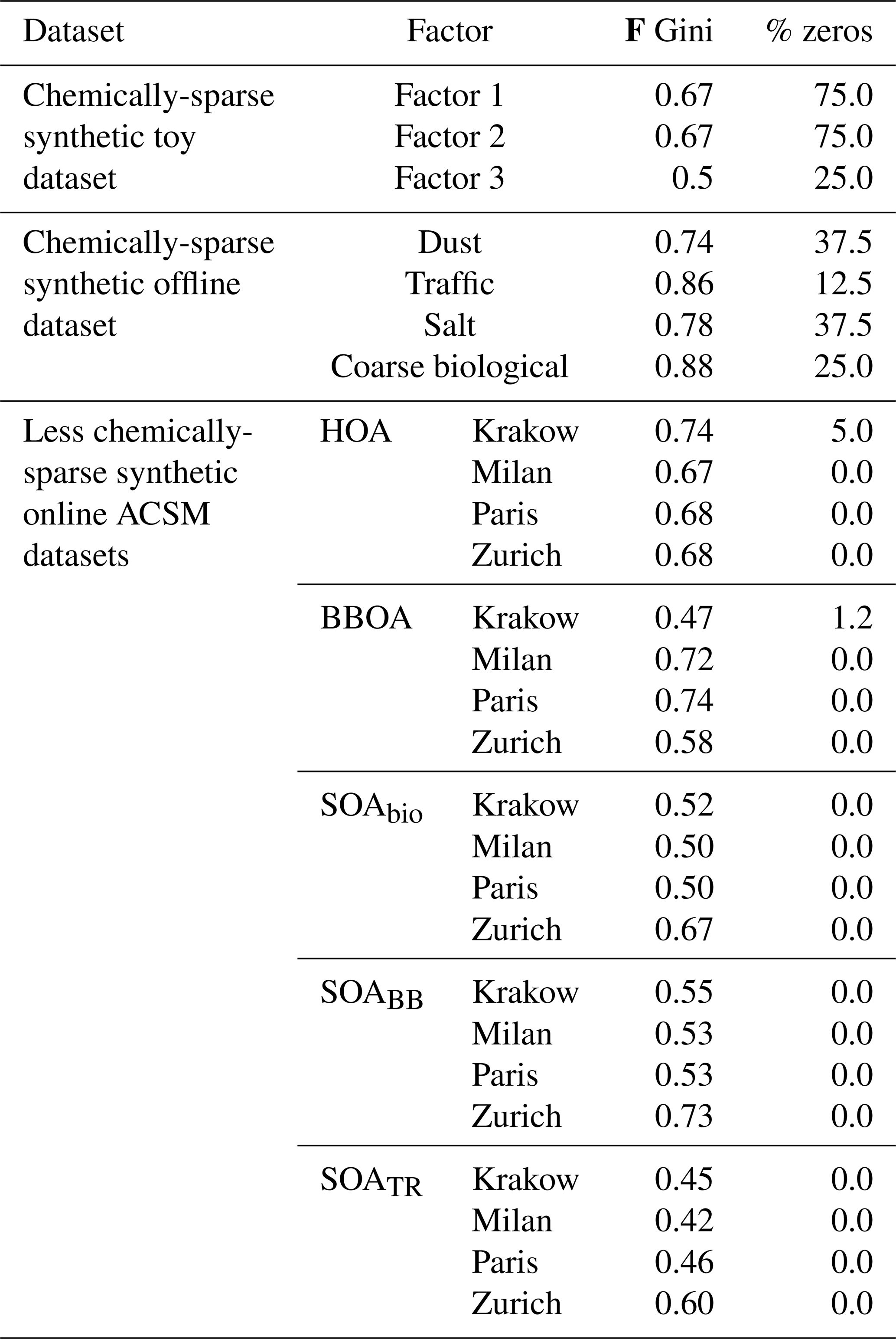
The datasets created for model experimentation can be divided into synthetic and real-world datasets. Synthetic datasets are artificially created with the purpose of knowing the F, G, to test model accuracy retrieving these matrices with respect to the truth and these have been widely used for source apportionment validation in the last decades (Park et al., 2002; Brinkman et al., 2006; Belis et al., 2015; Via et al., 2022; Rusanen et al., 2024). In order to challenge the models gradually, we created three synthetic datasets with increasing degrees of complexities (toy, offline, online ACSM synthetic datasets). Additionally, a real-world chemically sparse dataset was also used to test the results. Although the truth factorisation is unknown and the results cannot be directly verified, the model's factorisation can be assessed environmentally or based on indicators on the goodness of fit. The different datasets have different levels of sparsity, as can be seen in Table 2, that the models with the horseshoe prior should aim to replicate. The time resolution of modelled OA sources, used both in the chemically-sparse toy dataset and the chemically less sparse datasets, is 1 h. The time resolution of offline datasets, used in the chemically sparse synthetic offline dataset and the chemically-sparse real-world offline dataset is 1 d.

Table 2 Profile sparsity metrics for the truth of synthetic datasets.

2.4.1 Chemically-sparse toy dataset

A simplistic synthetic toy dataset was designed as a deliberately simplified test case to perform basic control and performance tests, rather than to reproduce any realistic atmospheric scenario. It was devised by creating three very simple and sparse profiles and using three time series (HOA, SOA_bio, BBOA) from modelled source time series of the city of Zurich (Rusanen et al., 2024, time resolution of 1 h) in order to test how sparsity priors act on very uneven species contribution. Although it is based on ACSM-like time series and therefore reflects some of the temporal properties of such measurements, the three included sources do not represent combinations that would be expected in a real-world environment since this toy dataset is intended solely for methodological testing purposes. In addition, the source profiles were intentionally designed to be highly simplified in order to facilitate an immediate visual assessment of the model fitting. For these reasons, the extracted components were not assigned environmental labels, but were instead referred to generically as Factor 1, Factor 2, and Factor 3.

Then, F and G were multiplied to generate Z, and some gaussian error with standard deviation σ was added to each component to generate a realistic X matrix. The uncertainties matrix σ was designed as a sixth of the X values plus Gaussian noise. With this arrangement, the models can be applied conventionally to the X, σ matrices and the modelled F and G, can be compared to the original truth F, G, which will be referred hereinafter as F₀ and G₀, displayed in Fig. S2.

2.4.2 Chemically-sparse synthetic offline dataset

We created a synthetic offline filter dataset, mimicking the filter-based measurements input matrices, in order to test the accuracy of the models in these kinds of datasets. This dataset mimics the concentrations on the coarse fraction (PM₁₀–PM_2.5) as collected by a high-volume sampler on the Zurich-Kaserne site (Grange et al., 2021) including the following chemical species: OC, Al, Na, Mg, Cl, K, Ca, S, Fe, Cu, Zn, Mn, Sb, Ba, mannitol, arabitol. In the original real-world dataset, data obtained with two series of samples (PM₁₀ and PM_2.5) were subtracted in order to focus on the coarse source apportionment, since the main emission sources of these elements and organic species stem from mechanical processes leading to major coarse models. It was created by crafting first the F and G, then multiply them and creating X and σ. The F matrix was slightly modified from that proposed in Manousakas et al. (2025), making the chemical profiles slightly sparse by zeroing the non-relevant species in each of the factors (dust, traffic, salt, coarse biological). The G matrix was composed of the time series of:

• Dust: modelled PM₁₀ dust (Vasilakos et al., 2026) converted to coarse with the Al_PM10 vs. PM₁₀ ratio from Grange et al. (2021).

• Traffic: modelled PM₁₀ copper (Upadhyay et al., 2025) converted to coarse with the Cu_PM10 vs. PM₁₀ ratio from Grange et al. (2021).

• Salt: coarse Na+Cl (Grange et al., 2021) converted to PM concentrations and multiplied by an arbitrary number (3 in this case match the concentrations of the sea salt factor in the original dataset).

• Coarse biological: coarse Arabitol+Mannitol (Grange et al., 2021) converted to PM concentrations and multiplied by 3, similarly as for the salt factor.

This dataset will be called “offline synthetic dataset”. Another more simplistic dataset was prepared similarly but using Al and Cu for dust and traffic factors, respectively, in the same way as in the salt or coarse biological factors, i.e. omitting the use of modelled data. This dataset will be hereinafter named “Purely-measurement-based offline synthetic dataset” and its modelling results will be described in Sect. 3.2. Once the F and G matrices were created, X was calculated by their multiplication and the addition of Gaussian noise with amplitude σ. The uncertainties matrix σ was generated as in Grange et al. (2021) multiplied by 2 to balance the signal-to-noise ratio to the datasets in Manousakas et al. (2025). The matrices F, G of this dataset are displayed in Fig. S3.

2.4.3 Chemically sparse real-world offline dataset

A real-world dataset was employed to test the current models applicability in campaign measurements. This dataset was originally used for source apportionment in Manousakas et al. (2025) and Grange et al. (2021) and consists of PM_10–2.5 samples at five Swiss National Air Pollution Monitoring Network (NABEL): Basel, Bern, Magadino, Payerne, and Zurich. The measurements were taken in the June 2018–July 2019 period every fourth day and using Digitel high-volume samplers. During the sampling campaign PM₁₀ and PM_2.5 were collected and the respective concentrations were subtracted to generate the coarse (PM_10–2.5) concentrations. These samples include: (i) OC concentrations, measured through the thermal optical transmission (TOT) EN16909 method with the EUSAAR2 temperature protocol; (ii) elemental concentrations (Al, Fe, Cu, Zn, Mn, Sb, Ba, Sr, Bi, Pb) measured by inductively coupled plasma atomic emission spectrometry (ICP-AES) and inductively coupled plasma mass spectroscopy (ICP-MS); (iii) water soluble inorganic ion concentrations (Ca⁺, Cl⁺, Mg⁺, K⁺, Na⁺), determined by ion chromatography (IC); (iv) Organic species (mannitol, arabitol) determined by a high-performance liquid chromatographic method followed by pulsed amperometric detection (HPLC-PAD). The uncertainties of these species were calculated as in Grange et al. (2021).

2.4.4 Chemically less sparse synthetic online ACSM datasets

With the aim of recreating more complex real-world datasets to test the models, we generated 6 datasets for four European cities: Krakow, Milan, Paris, and Zurich. The objective was to recreate OA matrices as given by a mass spectrometer instrument like Q-ACSM, for which there are plenty of real-world source apportionment studies in the literature. The G matrix was created from OA sources time series generated through the regional air quality model CAMx (Comprehensive Air Quality Model with Extensions) as previously published by Jiang et al. (2019). The five sources of these datasets were hydrocarbon-like OA (HOA), related to traffic emissions, biomass burning OA (BBOA), biogenic SOA (SOA_bio), biomass burning SOA (SOA_bb), and traffic SOA (SOA_tr). To ensure seasonal representativity while keeping computational costs low, datasets included the first two weeks of every second month of 2011 (January, March, …). The relative concentrations of these datasets are shown in Fig. S5. This figure shows the highest seasonal OA variation for the city of Milan and the lowest for Zurich. In terms of sources, the most seasonally stable sources, overall, are HOA and SOA_tr in contrast to the remarkable variability of BBOA and SOA_bio. The profiles used to create the species matrix F were those in Table S2 for primary sources (HOA, BBOA). For secondary sources, the profiles from the European megacity dataset presented in Rusanen et al. (2024) were used for the Zurich city, which were slightly perturbed for the other cities due to the limited availability of these sources' profiles in the literature.

The X matrix was obtained by multiplying the F and G submatrices and adding Gaussian noise. The procedure to calculate the error matrix for such datasets is described in Via et al. (2022) and the dataset used to calculate the error matrix is that from the Zurich site, which ranges from February 2011 until December 2011.

Lastly, a sensitivity analysis was carried out by slightly modifying the original F, G matrices upon which the X, σ matrices were subsequently created. The first Zurich dataset (period 1–14 Sepetember 2011) was used for this purpose and we chose to perturbate one factor only (HOA). The F, G submatrices were perturbed independently upon the expression:

$$\begin{array}{}\text{(16)}& G_{\mathrm{HOA}}^{\prime }=G_{\mathrm{HOA}}\cdot N(\mathrm{1},{\mathit{\sigma }}^{\prime })F_{\mathrm{HOA}}^{\prime }=F_{\mathrm{HOA}}\cdot N(\mathrm{1},{\mathit{\sigma }}^{\prime })\end{array}$$

where we used ${\mathit{\sigma }}^{\prime }=$ [0, 0.1, 0.2, 0.3, 0.4, 0.5] to create different degrees of perturbation. The profiles in F were normalised after that process. It must be noted that the perturbation is more relevant on F than in G since a given σ' in the aforementioned range is more comparable and impactful on the profile contributions, bounded to 1, than on the unbounded time series timepoints. Consequently, within this framework, we obtained 6 G-perturbed and 6 F-perturbed input matrices. Both BAMF and BAMF+HS models were run with all these input matrices and their subsequent HOA results were compared to the original truth in order to comprehend the sensitivity of the models upon time series and profile perturbations.

3 Results

3.1 Chemically sparse synthetic toy dataset

Here, we introduce the evaluated models relying on unrealistically simplified toy data with the purpose of showcasing the performance of the horseshoe prior introduction to BAMF (Fig. S2) and the alternative factorisation methodologies, which are discussed in Sect. S3.1.

Table 3 Toy experiment statistics of (a) Factorisation performance. (b) Comparison to truth. Green sequential colorscales represent variables whose larger value leans to a better performance and the blue-to-red divergent colorscales (centered at 1, in white) represent $G/G_{\mathrm{0}}$ divergence with respect to 1. Red bars in (a) depict deviations from the ideal 0 value.

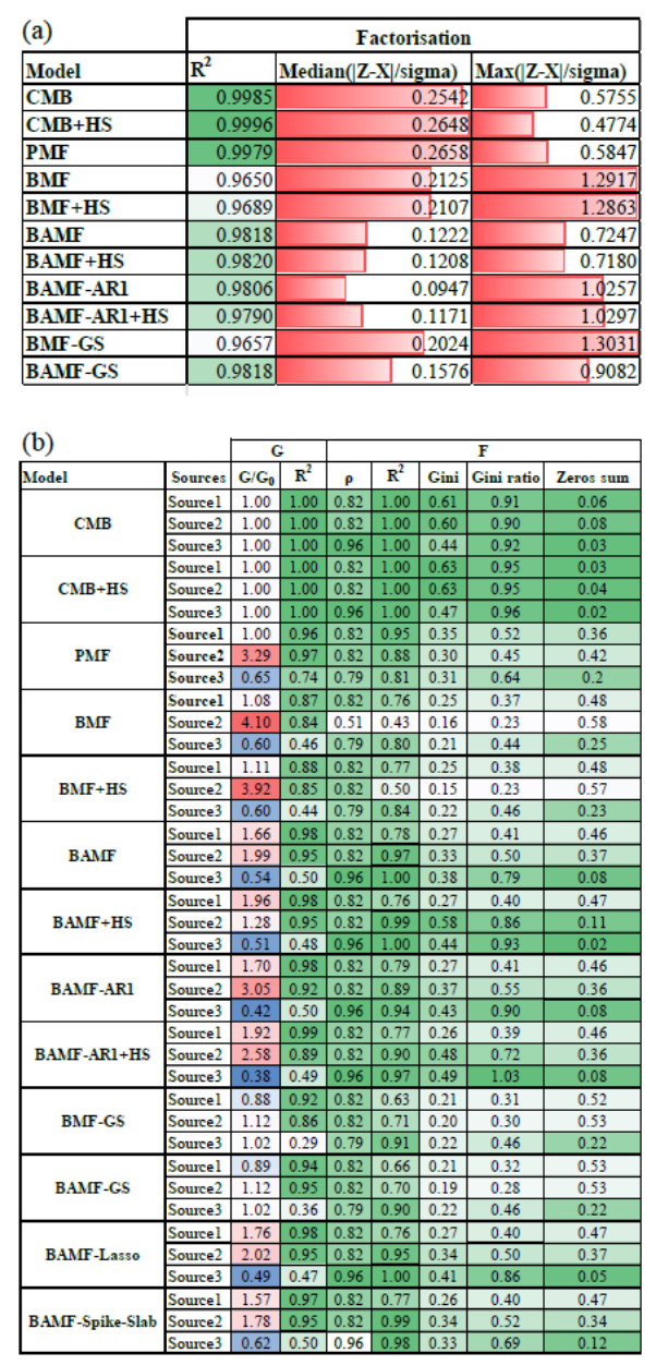
In the first evaluation step, we assess the performance of the horseshoe prior under the assumption that the source matrix G is known, in order to isolate its effect on the estimation of F. Figure 1 shows the distribution of each F component for CMB with and without the horseshoe prior (CMB, CMB+HS, respectively, Table 1). The distributions shown account for all the variability across samples of each F component for both models, and the truth is shown as a marker in the x-axis since it is a point value to be compared to the centers of the distributions. The presentation of the CMB and CMB+HS distributions aims to demonstrate the sparsity-inducing role of the horseshoe prior, which enforces shrinkage of the F component toward zero; this effect is more readily discernible when a strongly guided G matrix is used to isolate the evidence of sparsity. Figure 1 showcases the horseshoe prior power to generate sparsity in F components, shrinking more strongly the lowest signals to zero than CMB and, as a consequence, enlarging the most prominent signals. Table 3 shows how the Gini metric is consistently higher for CMB+HS with respect to CMB, supported by a higher Gini ratio and lower zero truth metric reflecting the sparsification of profiles and higher similarity to truth. The RMSE compared to the truth for the profiles improved with the horseshoe prior applied for all three factors (for CMB and CMB+HS, respectively: $\mathrm{1.2}\times {\mathrm{10}}^{-\mathrm{4}}$, $\mathrm{3.8}\times {\mathrm{10}}^{-\mathrm{5}}$ for F1; $\mathrm{1.86}\times {\mathrm{10}}^{-\mathrm{4}}$, $\mathrm{5}\times {\mathrm{10}}^{-\mathrm{5}}$ for F2; $\mathrm{3.3}\times {\mathrm{10}}^{-\mathrm{5}}$, $\mathrm{1}\times {\mathrm{10}}^{-\mathrm{5}}$ for F3). Hence, the sparsity introduced in F through the regularised horseshoe prior successfully improved the profile description of the solution.

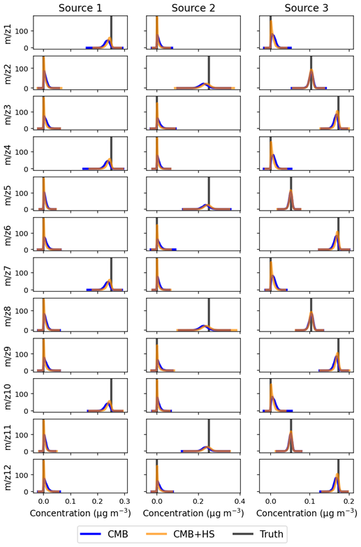
Figure 1 Distributions for the mass concentrations of all measured variables ($m/z$) for both CMB and CMB+HS (solid lines) compared to truth (markers).

In the next evaluation step, we test the various models assuming no prior knowledge. Figure 2 shows the results of PMF, BAMF, and BAMF+HS models on the toy dataset and Table 3 shows their factorisation performance and comparison to truth metrics. In terms of factorisation, median relative errors are better for BAMF+HS and BAMF than for PMF, but their maximum errors are higher and the Pearson coefficients slightly lower, all this entailing comparable factorisation performances. All models generally adapt well to the truth features, but they present non-negligible differences. PMF results better resemble the truth in terms of GR², but it is the model whose $G/G_{\mathrm{0}}$ differs from 1 the most, accumulating the greatest error (2.64), followed by BAMF (2.10), while BAMF+HS exhibits the smallest deviation (0.81), indicating the highest overall accuracy. In terms of profiles, the BAMF+HS model is the closest to the truth both in terms of ρ and R², especially for the second and third factors for which the sparsity introduction results are advantageous with respect to BAMF results. Consistently, the Gini ratios of the inferred solutions relative to the truth are markedly closer to unity for BAMF+HS (range 0.40–0.93) than for PMF (0.45–0.64). The sparsity effects can also be seen in Fig. S5, in which the horseshoe shrinkage is evident for the low $m/z$s allowing in turn the larger $m/z$s to retain more mass, hence resembling better the truth profiles. Taken together, these results indicate that BAMF+HS not only promotes sparsity, but does so in a chemically consistent manner, leading to a more accurate mass apportionment across factors, despite a slightly reduced time-series correlation for the third factor. However, the BAMF+HS could not shrink down the lowest signals in Factor 1, likely because their contribution estimated by the mass balance and the autocorrelation restrictions of this model made it unclear for the horseshoe to shrink them down completely. With this result, this toy dataset depicts the capacities and limitations of the horseshoe implementation on BAMF: it is capable to sparsify effectively only the signals which are close enough to zero as given by the restrictions of the BAMF model.

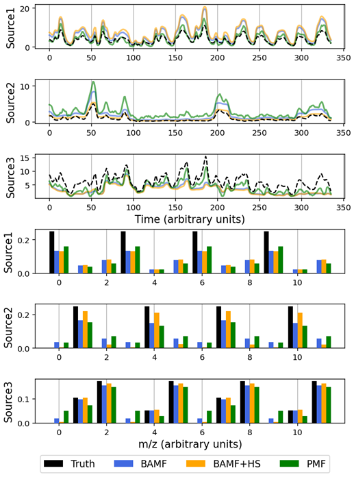
Figure 2 Source apportionment results for the toy dataset obtained using PMF, BAMF, and BAMF+HS, compared against the true solution (black bars). (a) Factor time series. (b) Factor profiles.

While other sparsity priors exist (e.g. Lasso and Spike-and-slab priors (Fig. S6, Tables 3, S3)), our tests show that the BAMF+HS model is most effective in shrinking unnecessary contributors to F. Hence this prior will be used onwards. This is evidently portrayed by the Gini ratio, for which neither Lasso nor Spike-Slab achieve the signal shrinkage that the BAMF+HS does. Also, neither BAMF+Lasso nor BAMF+Spike-and-slab managed to sparsify the first factor. Additionally, different autocorrelation formulations were implemented with and without the horseshoe prior, showing worse performance than BAMF or BAMF+HS, respectively, as discussed in Sect. S3.1. This supports using the BAMF autocorrelation prior instead of the alternative AR(1) prior, G simplex formulation or lack of autocorrelation prior models, although these models are also tried on the other datasets to further highlight this.

3.2 Chemically sparse synthetic offline dataset

This synthetic offline dataset was used to assess the performance of different models on a proxy representation of atmospheric aerosol data, while maintaining the verifiability property inherent to synthetic datasets as described in Sect. 2.4.2. We performed source apportionment of the X matrix through the aforementioned Bayesian models and PMF, obtaining 4 factors fingerprints and time series. The dataset used in this source apportionment is expected to be much more sparse than ACSM-like datasets, hence it could better expose the capabilities and added value of the sparsity prior.

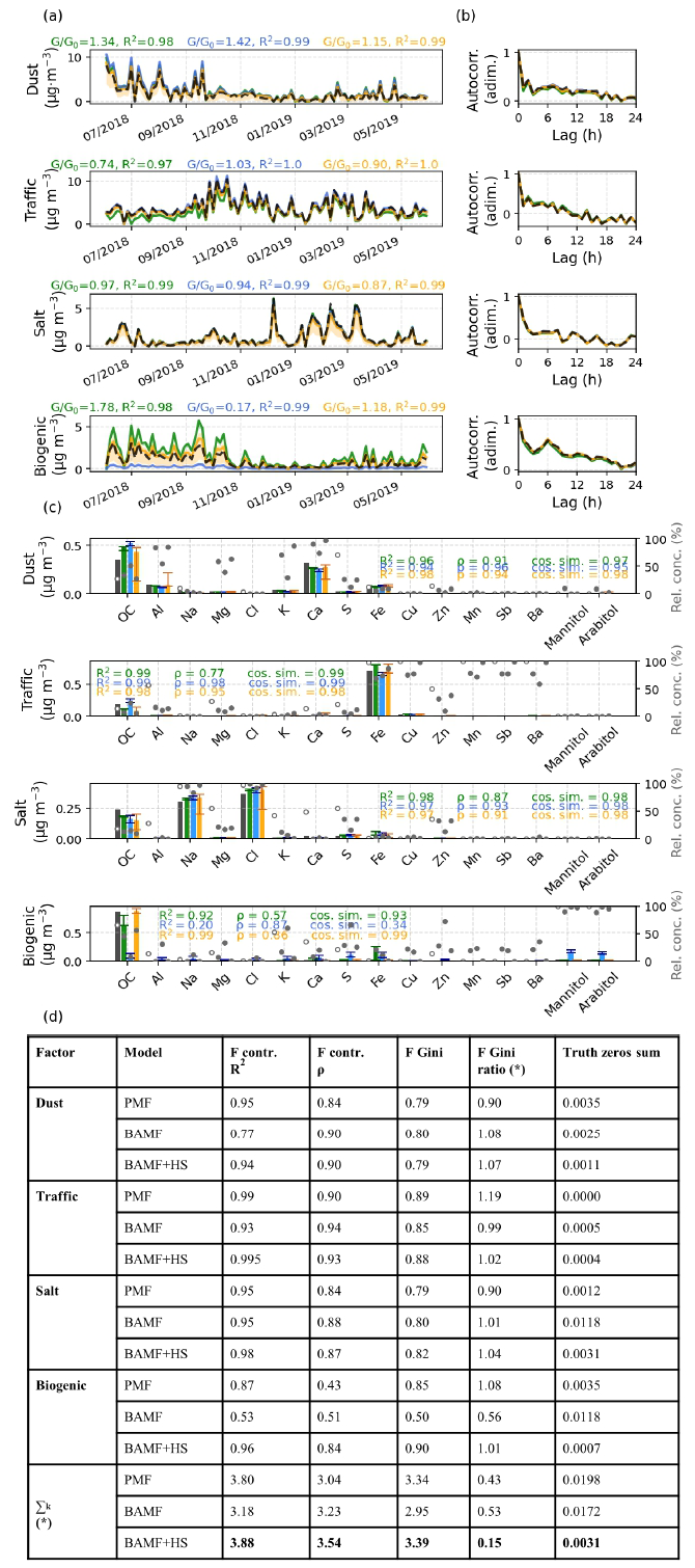
Figure 3 Synthetic offline dataset source apportionment results for PMF, BAMF, and BAMF+HS models. (a) Time Series. (b) Autocorrelation. (c) Profiles. (d) Table with additional metrics for comparison to truth. Bold numbers reflect the highest value amongst models. F contr. represents here the percentage of each factor in a given species. The sum row reflects the overall performance of the model for all sources for each statistic metric except for the ones marked with (*), in which the difference to 1 in absolute value is summed up.

To avoid initialisation failure, BAMF was run by initialising F as a normal distribution to ensure a more sturdy sampling. Model initialisation fails when no set of initial parameter values satisfying the model result in valid Bayesian solutions, and are usually solved by imposing more informative priors constraints on the model parameters. A t-test was run comparing the F, G factors from this slightly modified model and BAMF to ensure their similarity. Its results passed the t-test for all factors except for one factor, although it presented a R²=0.9990 correlation and only a 20 % of quantitative difference with that BAMF factor. Hence, one can assume that the model provides an acceptable level of agreement with BAMF, capturing the essential structure of the factors with only very minor deviations.

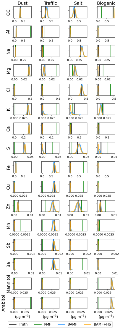
Figure 4 Profile components distribution for PMF, BAMF, BAMF+HS (colored lines) in comparison to the truth (black lines) on the real-world filters dataset. Rows represent the species of the source apportionment and columns represent sources.

Figure 3 presents the (a) time series (b) auto-correlation (c) profiles of the source apportionment solution for PMF, BAMF, BAMF+HS, (d) additional comparison to truth metrics, and Fig. 4 shows the histograms of the models F components estimation. The time series and autocorrelation show only slight differences between the models, the PMF being the most different to the truth in all factors except the salt one, as supported in Fig. 3d. Amongst factors, the coarse biological source is the most poorly reconstructed. If accounting for the sum of all factors GR²s and $G/G_{\mathrm{0}}$, in the last row of Fig. 3d, the most accurate model is the BAMF+HS, followed by PMF and then BAMF. In terms of profiles, the best overall model performance depends on the metric, F Spearman correlation coefficient being highest for BAMF and R² and cosine similarity correlation coefficients for BAMF+HS. This fact, accompanied by Gini being the highest for BAMF+HS and the closest to 1 Gini ratio, indicates that the extreme values of the profile (i.e. maximum and zeros species contributions) are closer to truth for BAMF+HS, whose extreme contributions would be less relevant in the Spearman correlation coefficient. Considering the Truth F zeros sum metric, the horseshoe shrinkage is visibly sparsifying most of the low signals whilst BAMF and PMF present non-zero contributions for species whose contribution in this factor is null. Hence, the BAMF+HS model would effectively promote the profiles sparsity which it was intended for.

However, the favourable results of BAMF+HS in comparison to the other models could be a dataset-dependent finding, related to the properties of the created synthetic dataset. The purely-measurement-based offline synthetic dataset, whose performance statistics are shown in Table S4, shows that PMF overperforms BAMF+HS, presenting slightly higher F and GR² and better $G/G_{\mathrm{0}}$. This could indicate that the optimal model selection might be dataset dependent. However, the source time series of this very simplistic dataset are fully correlated with some species time series, since they are used to generate factor time series, which makes it a very redundant dataset. In this scenario, the source apportionment comparison might still be valid, but it is not the perfect showcase for RMs testing due to the excessive source correlation with species. We found it valuable to present different model performances on different datasets, which in atmospheric measurements, can suffer from artefacts complicating the behaviour of some models.

In the same way, the alternative autocorrelation priors models were also tried and will be thoroughly discussed in Sect. S3.2. However, overall, the BAMF+HS model is the one providing the best source apportionment results for this offline dataset, taking advantage of the sparsity to upgrade both profiles and time series accuracy.

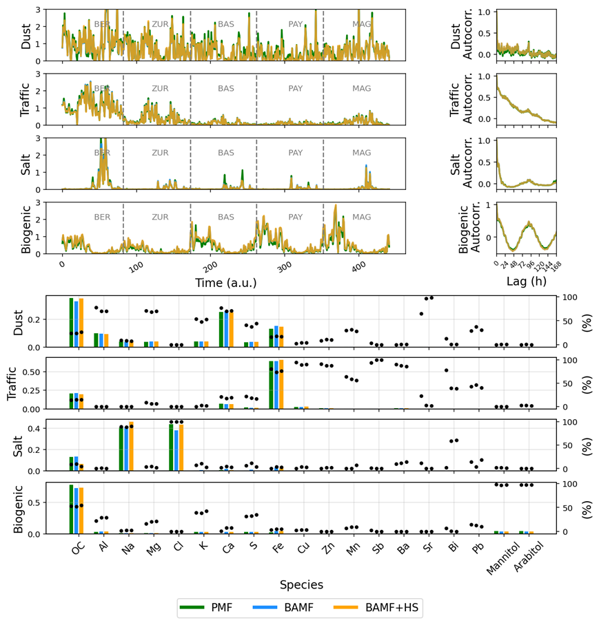
Figure 5 Comparison of PMF, BAMF, BAMF+HS for the real-world filters dataset. From left to right and top to bottom: time series, autocorrelation, and profile plots. The dots in the profiles (right axis) show the contribution of each species to the source.

3.3 Real-world offline dataset

To test the models on real-world data and identify their limitations for more complex datasets, we tested the models in the real-world offline PM₁₀–PM_2.5 dataset described in Sect. 2.4.3. Since the truth is not accessible, the model performance can only be assessed upon environmental, factorisation-related, and coputational criteria. For this dataset, BAMF and BAMF-AR1 models presented initialisation issues preventing them from properly launching the models. To avoid this issue and make the model more robust, we implemented a prior in F so that its components are drawn from Gaussian distributions centered at zero and with a standard deviation of 1 so that we restrict values to be bounded to 1. This modification was not needed for the other models, which did not present initialisation issues.

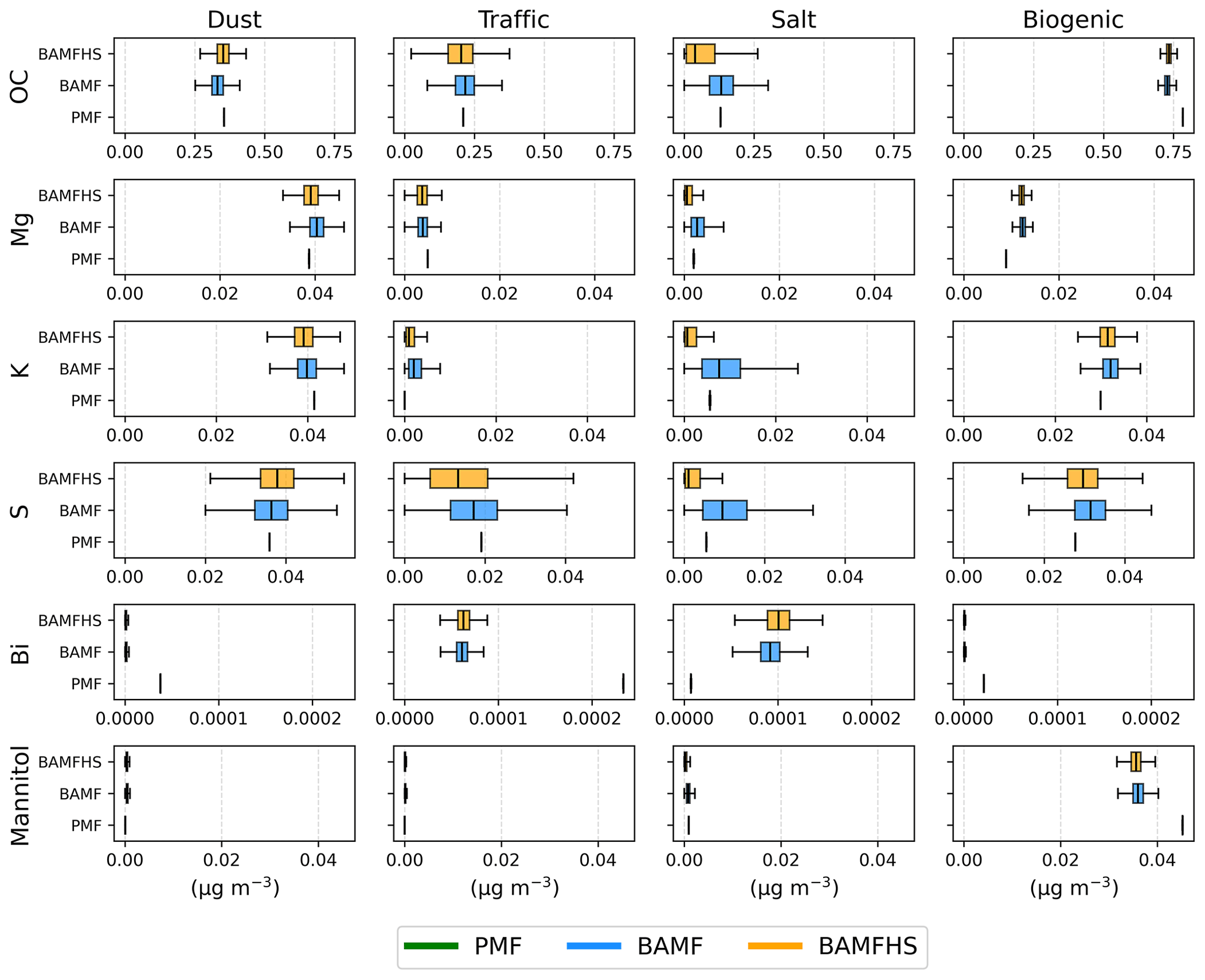
Figure 6 Boxplot distributions of individual profile components derived from PMF, BAMF, and BAMF+HS analyses for the real-world filter dataset. A complete comparison of all profiles is presented in Fig. S9.

Source apportionment results for PMF, BAMF, and BAMF+HS are shown in Fig. 5 and Table 4. Figure 6 shows the F distributions for these models, as a detail of Fig. S9a. Figures S6, S9a display very similar results for PMF, BAMF, BAMF+HS both in terms of F, G, and reconstruction metrics, and only some differences can be perceived for PMF, while BAMF and BAMF+HS histograms are almost overlapping in Fig. 6. However, the BAMF+HS profiles present a remarkable difference in terms of sparsity as seen in the F Gini metric, which is mostly the highest for BAMF+HS or equal, except for the biological factor for which PMF is slightly higher. For some species, the relative F components apportionment is more strongly suppressed by BAMF+HS than by BAMF or PMF, hence, their contribution on other profiles can be larger. This is clearly visible, for instance, for OC, Mg⁺, K⁺, S⁺, or mannitol, which are zeroed in the Salt factor and consequently are larger on the factors where these species are relevant. This is more evidently depicted in Figs. S9a and 6, where the distribution of F components is shown. For the aforementioned species, the horseshoe effect can be seen in the distribution, whilst BAMF and PMF are further from zero. This result thus highlights the potential benefits of sparsity introduction in matrix factorisation.

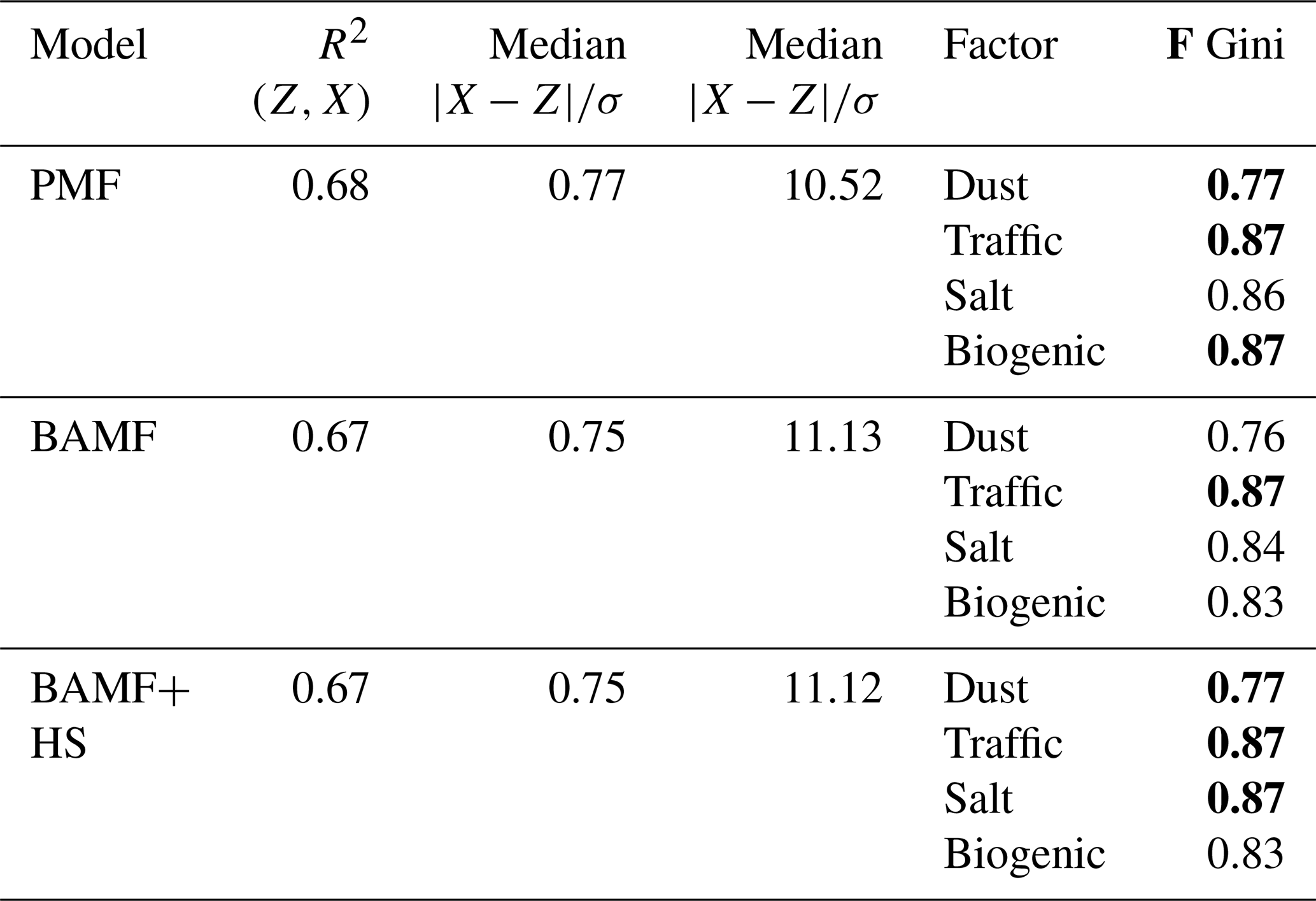
Table 4 Offline real-world dataset reconstruction and sparsity statistics. Bold numbers reflect the highest value amongst models.

The application of other autocorrelation priors was not advantageous with respect to the regular BAMF autocorrelation and even worsened the shrinkage power of the horseshoe prior as discussed in Sect. S3.3.

3.4 Chemically less sparse synthetic online ACSM datasets

The next step was to test these models on more realistic synthetic datasets. For that purpose, 6 datasets for 4 European cities (a total of 24 datasets) were designed with 5 factors in each of them (Sect. 2.4). We applied the 8 models under discussion (PMF, BMF, BMF+HS, BAMF, BAMF+HS, BAMF-AR1, BAMF-GS) to the 24 synthetic datasets and computed the summary statistics (the median of the ratios of G over the truth G, $G/G_{\mathrm{0}}$, the Pearson correlation of G with truth, Gr, and the Spearman correlation of F with truth, Fρ). All metrics over cities, datasets and sources are presented in Table S5, and an example for one site (Zurich) and one dataset (dataset 0, from 1 to 14 January 2019) is shown in Fig. S11 as an example of the results obtained by the three models in 1 out of the 24 datasets.

Figure 7 shows the model summary statistics over the 6 generated datasets for the four cities and Fig. S12 shows the factor-dependent statistics. In this case, the (not-squared) Pearson correlation coefficient was used to compare the results of the ACSM-like datasets more easily to those presented in Rusanen et al. (2024), which used this metric. Figure 7 shows a good agreement between models and the truth, with most solutions with correlations with truth for F and G above 0.7, similarly to Rusanen et al. (2024). However, there are clear differences amongst models and cities. PMF is performing worse in comparison to the Bayesian models, including BMF, the Bayesian analog to PMF in all datasets except for Milan. As shown in Table S5, PMF presents the highest $|Z-X|/\mathit{\sigma }$, the highest overestimations of G, and correlations of G and F are the lowest in comparison to other models except for the Milan dataset. In terms of $G/G_{\mathrm{0}}$, the model providing the best results are BAMF, BAMF-AR1, BAMF-GS, followed by their horseshoe versions. The BAMF+HS, presents slightly lower Fρ, FR², and the sparsity Gini metric ratio is not close to one, entailing the horseshoe prior did not successfully implement sparsity and the F accuracy did not improve. In terms of correlations with F and G, the models including the horseshoe prior present higher dispersion within a city with respect to the models without sparsity terms. Considering all the parameters, the models with the best overall performance are BAMF, BAMF-GS, and BAMF+HS.

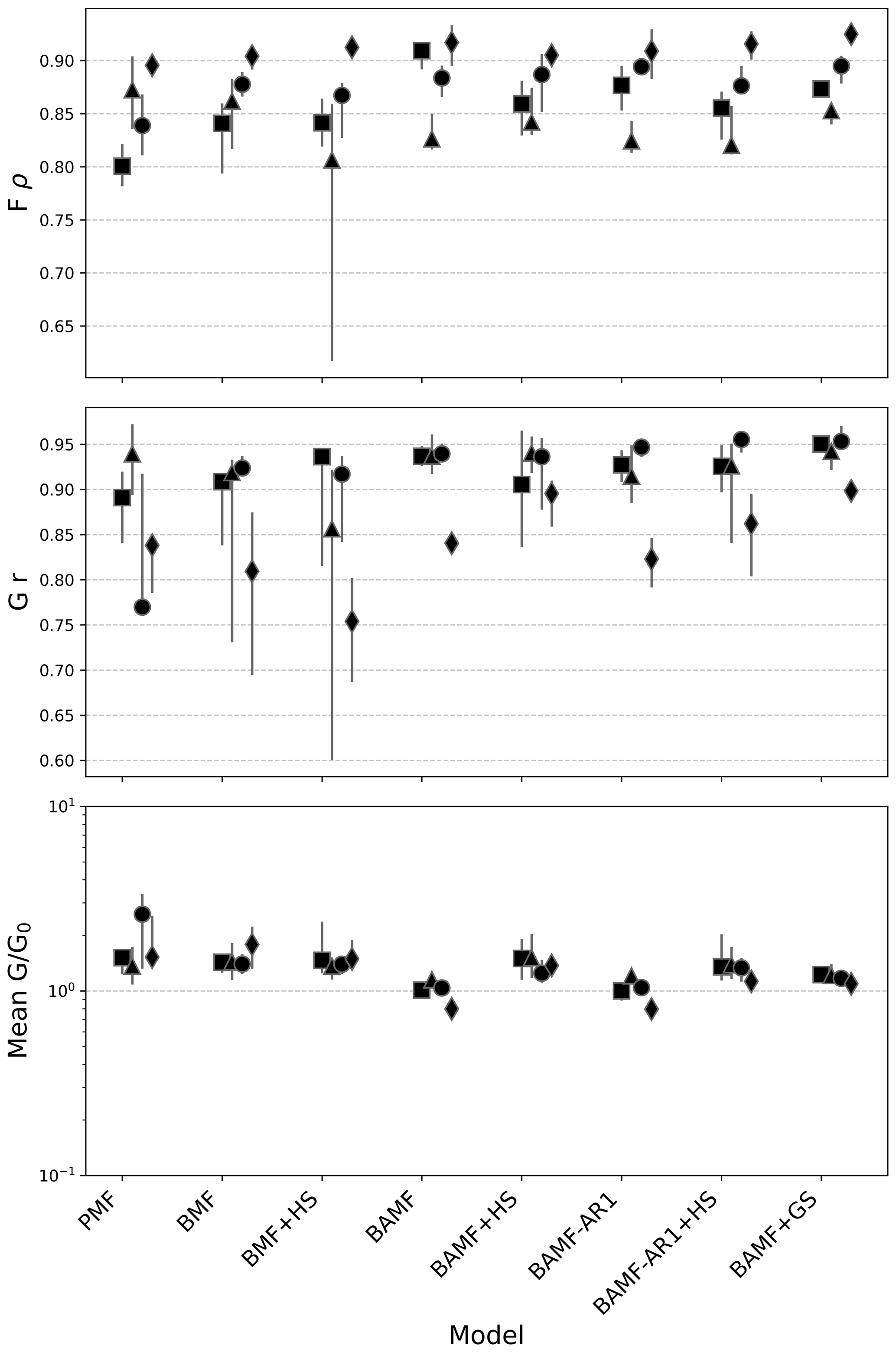
Figure 7 European cities synthetic datasets summary statistics; from top to bottom, median ratio time series with truth ($G/G_{\mathrm{0}}$), Pearson correlation coefficient of G with truth (Gr), Spearman correlation coefficient of F with truth (Fρ). The axis of the $G/G_{\mathrm{0}}$ plot is in logarithmic scale.

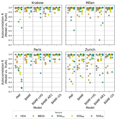
Figure 8 Pearson correlation of the autocorrelations of model solutions with the truth for all factors and all cities.

Figure S13 shows the autocorrelation for lags 0–168 h (half of the monthly measurement period) for all the sources and sites, displaying the cyclicity of the selected sources. In all cases, the short-term lags present very high autocorrelation, entailing that the similarity on adjacent timestamps is very high and decays over longer periods. Typically, and as presented on the figure, the autocorrelation of primary sources, with more marked daily cycles, decays faster than secondary sources, which evolve more steadily due to their slower reaction to emissions. Whilst HOA and BBOA present a very steady intradaily structure, with one or two maxima per day, the biogenic SOA presents one peak per day and the other two secondary sources may or may not present marked daily cycles. This different intra- and inter-daily structure amongst sources certainly challenges the models to resolve the source-dependent characteristic.

Figure 8 shows the autocorrelation from truth and the model outputs correlate (Pearson coefficient of determination) for each model and source in the 4 cities. Each dot represents one of the 6 datasets for each site, and colors represent the different sources. The results show that all models present very high Pearson coefficient ranges for G autocorrelations in comparison to truth except for PMF, which struggles with this dataset aspect due to the lack of accounting of self-correlation. In general terms, the best captured correlation by all models is that of SOABio, with the most regular cyclical patterns. The SOABB and SOATr autocorrelations seem to challenge the models further due to more irregular patterns, and for some datasets, their autocorrelation is poorly modeled. POA sources are generally accurately modelled, with HOA patterns slightly better captured than those from BBOA. Regarding models, the ones with better performance are BAMF-GS, BAMF, and BAMF+HS, with only slight differences between the last two. This observation suggests that the horseshoe prior addition does not significantly reduce the autocorrelation power of the BAMF.

Regarding sparsity, Fig. S14 depicts the lack of sparsity both for input and modelled data. This figure shows the truth's 5 lowest $m/z$ components as well as BAMF, BAMF+HS outcomes. The reference (truth) profiles do not present zeros but very small signals, as do many ACSM-like profiles in the AMS spectral database (Ulbrich et al., 2009, 2025). Both BAMF, BAMF+HS reflect this lack of sparsity, however, it could be expected that BAMF+HS would decrease the contributions of the lowest components. However, the sparsity introduction was not achieved as seen before in the lack of improvement of the Gini ratios. This lack of sparsity despite the enforcement through the horseshoe prior can be explained by the complexity of the data, which due to chain divergence, hinders the models performance. Figure S15 shows the model $\widehat{R}$, a typical Bayesian metric to evaluate the precision of Hamiltonian chains, computing the ratio between inter- and intra-chain variabilities. In any case results are very close to the ideal value, 1, so the validity of all models' solutions is assured. However, this plot reflects the deprecation of the solution with models when the horseshoe prior is applied. The horseshoe prior adds more complexity to the F with three more parameters compared to non-sparsity models which could be the cause of the increased model instability across chains.

Finally, a sensitivity analysis was run for the first Zurich dataset perturbating independently the original F, G matrices to different degrees, monitoring the correlation of the modelled F, G matrices to the original truth (Fig. 9). Subfigures (a) and (b) show how both in the case of the original F and G perturbations, the F accuracy drops immediately and analogously for both models, with a more sudden decay for G perturbations. Contrarily, the affectations in G (subplots (c) and (d)) are different for both models, with a steady decay for BAMF with G perturbations and a non-clear trend for F perturbations, whilst BAMF+HS correlation rests insensitive to F, G perturbations with an increasing/decreasing erratic behaviour. This result shows the reduced precision in G of BAMF+HS in comparison to BAMF due to the chain divergence issue, which, in any case, does not severely compromise its accuracy. This finding also explains the bigger variations for BAMF+HS with respect to BAMF in all the metrics shown in Fig. 8. Additionally, it showcases the general strong sensitivity of F determination opposite to the general robustness of G upon general X matrix perturbatio.

4 Discussion

This study aims to explore further BAMF capabilities and the benefits introduced through additional priors and/or modifications of the current model structure as given by Rusanen et al. (2024). The introduction of sparsity in source apportionment models was of particular interest to provide more distinct and concise source profiles which can, in turn, improve the time series accuracy. However, in real-world applications, it may also remove small but relevant signals along with noise. Therefore, comparison with BAMF results is recommended, leaving it to the user to decide whether the method's use is appropriate for their case.

Firstly, the use of the simplistic toy dataset highlighted the added value of the sparsity introduction through the horseshoe prior in the totally constrained experiment. In this controlled setting, the ground truth structure is well defined, allowing the effect of sparsity to be clearly isolated and the method performance validated. However, for an unconstrained experiment, sparsity was proven remarkably advantageous, but subject to the underlying matrix factorisation results. That is, the horseshoe prior in BAMF+HS effectively suppresses weak signals of F contributions as determined by BAMF, yet it fails to guide the model toward a more accurate or sparser solution when the initial BAMF estimate is suboptimal. Other sparsity priors, like Lasso and Spike-and-slab, were tried out but did not improve the regularised horseshoe performance.

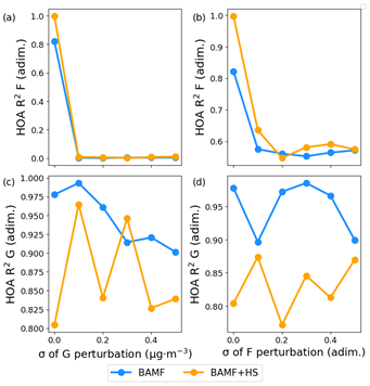
Figure 9 Squared Pearson coefficient of F, G matrix with original truth F, G matrices of the BAMF, BAMF+HS models with the degrees of perturbation in F and G.

The introduction of the regularised horseshoe prior in BAMF improved apportionment of offline synthetic and real-world datasets with respect to BAMF, promoting sparser profiles. The synthetic dataset comparison to truth was maximal for BAMF+HS, with sparser profiles and consequently better G accuracy. Its application also proved advantageous for the real-world dataset, despite not being able to be compared to the truth. In this case, improvements are assessed through increased profile distinctness and internal consistency rather than absolute accuracy. The results show a sparsity effect which provides more distinct profiles in comparison to PMF and BAMF. This result encourages the usage of the horseshoe prior for sparsity introduction in datasets whose solutions are expected to be strongly sparse, such as elemental datasets.

Subsequently, in the more complex and realistic European datasets, the sparsity introduction could not be effectively enforced. Although solution quality was not substantially compromised, the profiles remained non-sparse after applying the prior. This is likely due to model instability arising from the higher complexity of these datasets, which is further aggravated by the addition of the horseshoe prior, as it requires sampling a larger number of parameters. Moreover, the inherent nature of ACSM datasets – characterized by highly correlated species – might also contribute to this limitation, since the model struggles to disentangle overlapping sources when variables are strongly interdependent. The higher chain divergence found for the horseshoed models causes a drop in solution precision due to different landings on the solution space depending on the chain. This issue could be reduced by selecting chains a-posteriori upon user-defined criterion as is practiced in PMF. This is further confirmed by the insensitivity to G or F perturbations that are visible for BAMF+HS but not for BAMF. Nonetheless, given that ACSM-like factor profiles exhibit low sparsity in the literature, the use of sparsity priors in these datasets is less justified. Also, because usually ACSM profiles obtained in chamber or ambient experiments are not usually sparse, as seen in Ulbrich et al. (2009), the BAMF+HS is not as pertinent in these kinds of datasets as for filter-based datasets.

The sparsity conceptual framework could also be brought into PMF through the pulling equations, which can shrink down manually the expectedly low signals in a factor. However, this methodology requires that the user indicates the species that are intended to be zeroed, which introduces user-subjectivity to the problem. The BAMF+HS method, contrarily, acts globally, shrinking those species with lowest signals in favour of the matrix factorisation, hence no user intervention is needed. This makes the approach more objective but also less targeted, returning the factorization optimisation agency to the model. However, if the purpose were to enforce a shrinkage of a certain species as in the PMF case, this feature could also be implemented through the horseshoe method with minimal code modification.

The results of the other models tested (BAMF-AR1, BAMF-GS) did not show a significant improvement with respect to BAMF. The BAMF-AR1 contains another autocorrelation to parametrisation (STAN Development Team, 2025) which should allow for trend consideration, although this matter was not tackled in the current work and remains to be validated in future studies. The BAMF-GS seemed to capture slightly better the G variability in comparison to BAMF in the online datasets, but led to worse correlation to truth in the offline synthetic dataset. Nonetheless, it does not support enforcing sparsity in F, thereby reducing its effectiveness for profile adjustments.

5 Conclusions

This study presents a sparsity introduction technique for the Bayesian Autocorrelated Matrix Factorisation model (BAMF) which intends to condense source apportionment profiles removing noisy signals. The regularised horseshoe prior, a tool to promote sparsity in datasets, is introduced in BAMF (BAMF+HS) in order to narrow down the lowest signals in factor profiles while keeping the most significant ones regularised. The BAMF+HS model is built in STAN, an open-source framework for statistical modelling with Hamiltonian-Montecarlo Markov Chain sampling. In order to test the capabilities of the developed model, we generated three kinds of synthetic datasets to compare the model factorisation outputs to the truth factors, namely Toy, offline, and online synthetic datasets, each representing a progressively increasing level of complexity. Likewise, to confirm its usability to real-world data, BAMF+HS was also applied to a multi-site filter dataset. Given the opportunity to explore source apportionment with different types of datasets, we also tested other receptor models such as Positive Matrix Factorisation (PMF) and other BAMF-like Bayesian models. In the Bayesian framework, we tested a different formulation of the autocorrelation term (BAMF-AR1) and a permutation on the factorisation matrix logic (BAMF-GS).

The main result highlights can be summarised as:

• BAMF+HS has been shown to be advantageous to introduce sparsity in factor profiles for offline datasets and to not deprecate the solution for the more complex datasets mimicking Aerosol Chemical Speciation Monitor (ACSM) data. Other sparsifying priors tried out were not as effective in low-signal shrinkage.

• The BAMF+HS performance towards truth profile reconstruction was higher than for BAMF and PMF in the toy and offline synthetic datasets. Improving F typically led to a more accurate determination of G, highlighting the strong interdependence between the two factorisation matrices.

• The real-world dataset also shows a better description of sources through BAMF+HS in terms of matrix factorisation metrics and profile sparsification achievement.

• As shown in the toy dataset, the introduction of sparsity did not solve factorisation issues inherent to the underlying factorisation model.

• The BAMF+HS model does not create sparsity in ACSM-like datasets, which are originally, indeed, non-sparse. BAMF+HS is more unstable than BAMF for these more complex datasets as a result the higher chain divergence during Hamiltonian-Montecarlo Markov Chain sampling as suggested by the $\widehat{R}$ metric. However, the effects of the horseshoe prior do not affect the overall performance of BAMF or its autocorrelation accuracy.

• The alternative formulations for BAMF, BAMF-AR1 and BAMF-GS, did not show a significant improvement with respect to BAMF.

With all that, profile sparsity has been shown to substantially enhance the accuracy of source apportionment analyses, improving the separation of the chemical composition of sources. The BAMF+HS model succeeds in incorporating this property in profile fingerprints, especially in filter-based datasets. Using BAMF+HS in such datasets, the solutions reflect the sparsity of filter-based chemical profiles, hence, this newly introduced method is encouraged when source fingerprints are expected to be substantially sparse. However, for ACSM-like datasets, the sparsity is not fully achieved due to converge issues, although the quality of the solution is not substantially deprecated with respect to BAMF. With the aim of improving further source apportionment techniques, future research should be directed to enhance the robustness and generalisability of the BAMF+HS model across diverse data types. Moreover, continued exploration of the underlying properties of solution spaces (such as profile sparsity, time series autocorrelation) may provide valuable insights into disentangling complex source contributions through receptor modelling. In this regard, the Bayesian source apportionment framework offers a particularly suitable foundation, allowing for the integration of prior knowledge and uncertainty quantification in the inference process.