A Physics-Constrained Deep-Learning Framework based on Long-Term Remote-Sensing Data for Retrieving Vertical Distribution of PM_2.5 Chemical Components

The vertical distribution of PM_2.5 chemical components is crucial for identifying the causes of atmospheric pollution and its impact on climate change and extreme weather. By integrating long-term lidar measurements, deep-learning algorithms and a physics-constrained optimization method, this paper presents a novel lidar-based retrieval framework to obtain vertical mass concentration profiles of PM_2.5 chemical components for the first time. Identifiable components include sulfate (SO${}_{\mathrm{4}}^{\mathrm{2}-}$), nitrate (NO${}_{\mathrm{3}}^{-}$), ammonium (NH${}_{\mathrm{4}}^{+}$), organic matter (OM) and black carbon (BC), which extend beyond the component types that traditional remote-sensing retrievals can identify. A 1-year retrieved surface mass concentrations of these components closely aligned with the observations, with Pearson correlation coefficient values ranging from 0.87 to 0.97. The retrieval framework applied to varying non-training spatiotemporal scenarios showed moderate generalization capability, although a tendency toward underestimation is observed. Tower and aircraft-based field campaigns indicate that the retrieved and observed vertical profiles of these components exhibited consistent patterns in mass concentrations and proportions. Subsequently, an explainable method was incorporated into the retrieval framework to quantify the multivariate driving effects on vertical profile retrieval. Results showed that the extinction coefficient and representative indicators within physiochemical processes contributed significantly to mass concentrations of these components. Finally, a dataset of vertical mass concentration profiles of these components over six years in a Chinese megacity (Beijing) was generated by the retrieval framework, revealing the dominant roles of OM and NO${}_{\mathrm{3}}^{-}$ in PM_2.5 throughout the entire boundary layer across all seasons. As a result of the continued implementation of clean air policies in China, these components exhibited significant decreases during 2021–2022 compared with 2017–2018. Our retrieval framework offers a novel approach for acquiring vertical profiles of PM_2.5 chemical components, thereby providing a new perspective on elucidating the vertical evolution of atmospheric pollutants.

1 Introduction

PM_2.5 is a complex mixture composed of varying chemical components (Tao et al., 2017), mainly including sulfate (SO${}_{\mathrm{4}}^{\mathrm{2}-}$), nitrate (NO${}_{\mathrm{3}}^{-}$), ammonium (NH${}_{\mathrm{4}}^{+}$), organic matter (OM) and black carbon (BC). The diverse physiochemical properties arising from various chemical components yield distinct effects on the environment (Tan et al., 2018), climate change (Menon et al., 2002; Zhu et al., 2024) and human health (Kim et al., 2022). Vertical detection technologies have revealed that chemical components are primarily distributed at varying heights within the atmospheric boundary layer and contribute to environmental pollution through internal physiochemical processes (Morgan et al., 2009; Yang et al., 2024; Sun et al., 2015). Additionally, the proportion and vertical distribution of chemical components can regulate radiation flux at both the top of the atmosphere and at the surface by directly affecting light absorption and scattering, as well as the microphysical properties of clouds, thereby influencing climate change and extreme weather (Zhao et al., 2024). Consequently, characterizing the vertical structures of chemical components is essential for identifying the causes of PM_2.5 pollution and the response mechanisms related to climate change and extreme weather.

Field campaigns are widely conducted to obtain vertical profiles of PM_2.5 chemical components by mounting observation instruments on meteorological towers, aircraft, tethered balloons and unmanned aerial vehicles. However, these platforms are constrained by sparse detection sites and heights, limited flight schedules, and high observation costs (Dubey et al., 2022), hindering the time-continuous acquisition of vertical profiles of PM_2.5 chemical components within the whole boundary layer over a long-term period. Continuous remote-sensing lidar detection technologies with high temporal and vertical resolution serve as robust pathways for the constant identification of PM_2.5 and its components across all altitudes (Matus et al., 2025; Toth et al., 2022; Wang et al., 2022). Additionally, both satellite-based lidar and ground-based lidar networks, such as China Lidar Joint Observation Network (LiDARNET, https://lidar.pku.edu.cn/, last access: 25 July 2025), Asian Dust Network (AD-NET) (Sugimoto et al., 2005), Micro Pulse Lidar Network (MPLNET) (Welton et al., 2001), and European Aerosol Research Lidar Network (EARLINET) (Ansmann et al., 2003), provide remote sensing capabilities with extensive spatial coverage.

Retrieval algorithms for the lidar have been progressively developed over the past 20 years. Earlier studies utilized lidar depolarization ratios to identify dust and non-dust aerosols (Sugimoto et al., 2003; Tesche et al., 2009). Subsequently, additional lidar parameter constraints, such as multi-wavelength backscatter coefficient and lidar ratio, were incorporated to identify dust aerosol, water-soluble aerosols, black carbon, and sea salt based on the assumption of external mixing (Nishizawa et al., 2011; Nishizawa et al., 2017). Hara et al. (2018) considered the hygroscopic growth of water-soluble aerosols and their internal mixing with BC to mitigate the overestimation of BC retrieval (Hara et al., 2018). By integrating the ground-based lidar and sun-photometer, Wang et al. (2022) significantly increased the identifiable aerosol component types, including ammonium nitrate-like, water-insoluble organic matter, water-soluble organic matter, black carbon and fine-mode aerosol water content (Wang et al., 2022). However, the aerosol component type retrieved from existing lidar retrieval algorithms that utilize aerosol optical properties is not equivalent to the conventional chemical component type. Due to similar optical properties exhibited by PM_2.5 chemical components, the identification of chemical component types seems to be beyond the scope of remote-sensing retrieval (Wang et al., 2022). Moreover, the multiple parameterization assumptions introduced by existing lidar retrieval algorithms increase the uncertainties in component retrieval.

Data-driven machine learning can interpret the nonlinear relationships between PM_2.5 chemical components and various driving factors without the constraints imposed by the inherent properties of these components (Li et al., 2025a). Meng et al. (2018) utilized a random forest algorithm to predict national mass concentrations of SO${}_{\mathrm{4}}^{\mathrm{2}-}$, NO${}_{\mathrm{3}}^{-}$, organic carbon (OC) and elemental carbon (EC), achieving R² values ranging from 0.71 to 0.86 on a daily scale (Meng et al., 2018). Based on this algorithm, Lv et al. (2021) further achieved the hourly predictions of the aforementioned chemical components and NH${}_{\mathrm{4}}^{+}$ with R values of 0.71–0.81 (Lv et al., 2021). Subsequently, deep learning algorithms are employed to accurately characterize complex nonlinear relationships and effectively extract data features, thereby enhancing the predictive ability of hourly mass concentrations of PM_2.5 chemical components (Lee et al., 2023; Liu et al., 2023; Li et al., 2025a). However, current studies primarily focus on predicting the ground-level mass concentrations of PM_2.5 chemical components but cannot interpret the vertical distribution of these components. Furthermore, existing prediction models are susceptible to the quantity and quality of available training data due to the absence of physical constraints, limiting their spatiotemporal generalization capabilities.

In this study, we proposed a novel physics-constrained deep-learning framework that utilized lidar data to retrieve vertical profiles of five PM_2.5 chemical components (SO${}_{\mathrm{4}}^{\mathrm{2}-}$, NO${}_{\mathrm{3}}^{-}$, NH${}_{\mathrm{4}}^{+}$, OM and BC) for the first time. Our retrieval framework effectively mitigates the limitations of remote-sensing retrieval algorithms in identifying chemical components, as well as the deficiencies and limited generalization capabilities of purely data-driven machine learning techniques in characterizing vertical profiles of these components. Detailed descriptions of the retrieval framework and the data utilized are provided in Sect. 2., while Sect. 3 discusses the validation of the retrieval framework, the assessment of feature importance, and applications of this framework. Section 4 presents the conclusion.

2 Data and methodology

2.1 Data

2.1.1 Lidar measurement

The σ_bsc, 532 data for deep learning module training and PM_2.5 chemical component retrieving is obtained from a ground-based dual-wavelength polarization Mie lidar at the Institute of Atmospheric Physics (IAP), Chinese Academy of Sciences (CAS), Beijing (39.98° N, 116.38° E). This Mie lidar has consistently detected optical signals since 2017, offering a temporal resolution of 15 min and a vertical resolution of 6 m. The lidar specification parameters and data preprocessing are detailed in Sect. S1 (and Table S1) and Sect. S2 in the Supplement, respectively. The σ_bsc, 532 data from 8–15 February 2021 at 23 lidar sites in the North China Plain (NCP), provided by the China National Environmental Monitoring Center (CNEMC), were utilized to assess the spatial generalization ability. The multi-site data offers a temporal resolution of 5–20 min and a vertical resolution of 7.5 m. To generate an hourly resolution lidar dataset, minute-level data were resampled using a simple averaging method. Specifically, the arithmetic mean was calculated from all valid minute-level data points within each non-overlapping one-hour window aligned to the start of each hour (e.g., from 00:00 to 00:59).

2.1.2 Auxiliary data for Retrieval

The data of multiple meteorological parameters for deep learning module training and PM_2.5 chemical component retrieving can be obtained from the 5th Generation European Centre for Medium-Range Weather Forecasts (ECMWF) ReAnalysis (ERA5, https://cds.climate.copernicus.eu/datasets, last access: 25 July 2025), which provides the hourly data on pressure levels (1000–1 hPa) from 1940 to present with a spatial resolution of 0.25°×0.25°. The data of fine soil, coarse mass and fine sea salt for physics-constrained optimization can be obtained from 4th Generation ECMWF Atmospheric Composition Reanalysis (EAC4, https://ads.atmosphere.copernicus.eu/datasets, last access: 25 July 2025), which provides the 3 h data on pressure levels (1000–1 hPa) from 2003 to 2024 with a spatial resolution of 0.75°×0.75°. The mass concentration (µg m⁻³) of fine soil is approximately estimated by the mixing ratio (kg kg⁻¹) of dust aerosol with a diameter of 0.03–0.9 µm. The mass concentration (µg m⁻³) of coarse mass is approximately estimated by the mixing ratio (kg kg⁻¹) of dust aerosol with a diameter of 0.9–20 µm. The mass concentration (µg m⁻³) of fine sea salt is approximately estimated by the mixing ratio (kg kg⁻¹) of sea salt aerosol with a diameter of 0.03–5 µm. The pressure levels (hPa) of ERA5 and EAC4 are converted to geometric heights (m), and the 3 h EAC4 data is converted to hourly data through a linear interpolation method. The grid cells of EAC4 and ERA5 that contain the lidar sites were extracted using the k-nearest neighbor search method based on longitude and latitude data (Friedman et al., 1977). The lidar data and the reanalysis data were interpolated onto a preset vertical grid with a height range of 50 m to 3 km using linear interpolation. The preset height information is presented in Sect. S2.

2.1.3 Surface observations

Ground-level mass concentrations of NH${}_{\mathrm{4}}^{+}$, SO${}_{\mathrm{4}}^{\mathrm{2}-}$, NO${}_{\mathrm{3}}^{-}$, OM and BC at the Beijing lidar site (39.98° N, 116.38° E) were collected for training the deep learning module and validating retrievals by a high-resolution time-of-flight aerosol mass spectrometer, with a temporal resolution of 1 h, covering the periods from 1 January 2021, to 31 March 2022, and 1 June to 31 August 2022. Ground-level mass concentrations of the five PM_2.5 chemical components at 23 non-training NCP sites were provided by CNEMC. Besides, ground-level PM_2.5 mass concentrations, approximately equal to the sum of the mass concentrations of the five chemical components, are available on CNEMC data release website (https://www.cnemc.cn/, last access: 25 July 2025).

2.1.4 Aircraft-based and tower-based measurements

The aircraft-based vertical profiles for retrieval independent verification were sampled in a flight experiment at an airport site in Shijiazhuang (37.54° N, 114.35° E). The flight time schedules (LT, local time) are detailed in Table 1. The tower-based vertical profiles at altitudes of 16, 102 and 280 m were sampled at a 325 m meteorological tower located at the IAP, CAS in Beijing (39.98° N, 116.38° E) for 10 d (27 and 30 December 2023; 2, 5, 9, 12, 15, 18, 24, and 27 January 2024). A flow sampler with a flow rate of 42.8 L min⁻¹ and the 47 mm quartz filter membranes were utilized to collect PM_2.5 chemical component samples in the aircraft-based and tower-based sampling experiments. Furthermore, the 325 m tower-based vertical profiles from 30 December 2018 to 2 January 2019 were also collected from Lei et al. (2021)'s study.

Table 1 Flight time schedules (LT, local time), corresponding surface temperature and relative humidity.

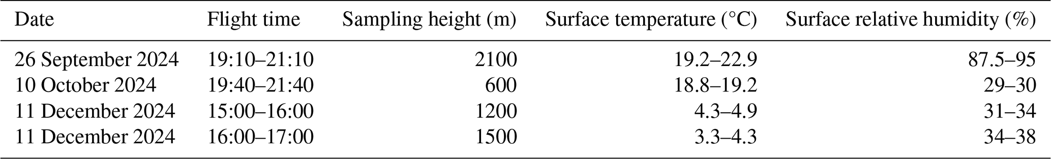
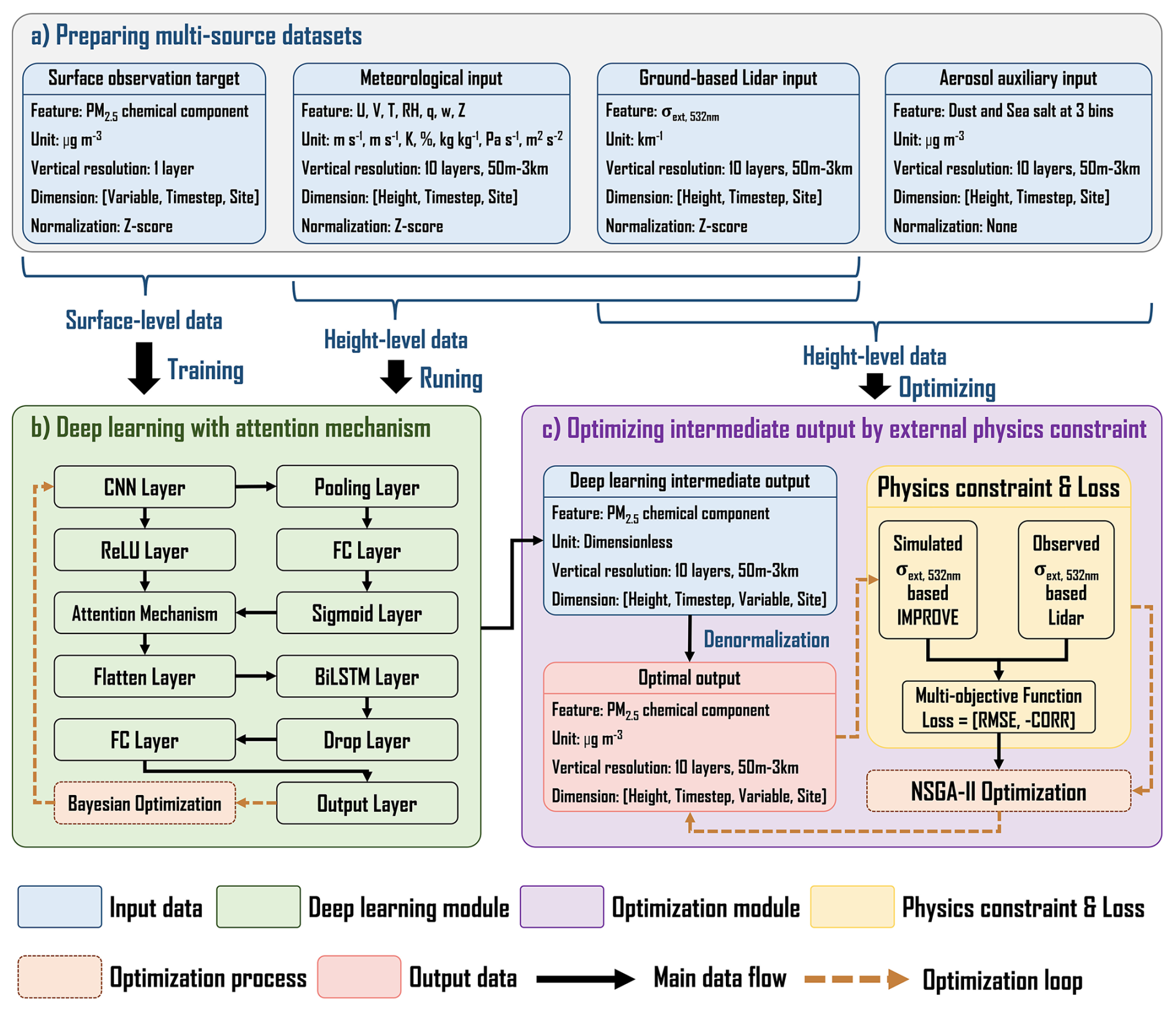
Figure 1 Remote-sensing retrieval framework for vertical distribution of five PM_2.5 chemical components (NH${}_{\mathrm{4}}^{+}$, SO${}_{\mathrm{4}}^{\mathrm{2}-}$, NO${}_{\mathrm{3}}^{-}$, OM and BC). (U: U-component wind; V: V-component wind; T: Temperature; RH: Relative Humidity; q: Specific Humidity; w: Vertical Velocity; Z: Geopotential; σ_ext, 532: Aerosol Extinction Coefficient at 532 nm; CNN: Convolutional Neural Network; ReLU: Rectified Linear Unit; FC: Fully Connected; BiLSTM: Bidirectional Long Short-Term Memory; IMPROVE: Interagency Monitoring of Projected Visual Environment; NSGA-II: Non-dominated Sorting Genetic Algorithm II).

2.2 Methodology

2.2.1 Retrieval framework

This paper proposed a novel retrieval framework for retrieving the vertical concentration profiles of five PM_2.5 chemical components (NH${}_{\mathrm{4}}^{+}$, SO${}_{\mathrm{4}}^{\mathrm{2}-}$, NO${}_{\mathrm{3}}^{-}$, OM and BC) from the lidar aerosol extinction coefficient at 532 nm (σ_bsc, 532). As shown in Fig. 1, the retrieval framework mainly consists of a deep learning module and a physics-constrained optimization module. The input datasets of the deep learning module include the surface observation data, meteorological data and ground-based lidar data (Fig. 1a). Specifically, the aerosol extinction coefficient at 532 nm (σ_bsc, 532) and multiple meteorological parameters (u-component wind, v-component wind, temperature, relative humidity, specific humidity, vertical velocity and geopotential) serve as input features, while the concentrations of the five PM_2.5 chemical components (NH${}_{\mathrm{4}}^{+}$, SO${}_{\mathrm{4}}^{\mathrm{2}-}$, NO${}_{\mathrm{3}}^{-}$, OM and BC) serve as target features. The deep learning module (Fig. 1b), mainly consisting of the Convolutional Neural Network (CNN), Bidirectional Long Short-Term Memory (BiLSTM), attention mechanism and Bayesian optimization, is utilized to establish the nonlinear relationship between input and target features. The input datasets of the physics-constrained optimization module include the ground-based lidar data, aerosol auxiliary data and deep learning intermediate output (Fig. 1a, c), which provide fundamental input for establishing a multi-object function based on the Interagency Monitoring of Projected Visual Environment (IMPROVE) equation. The physics-constrained optimization module incorporates the multi-object loss function with the Non-dominated Sorting Genetic Algorithm II (NSGA-II) to implement external physical constraints (Fig. 1c), thus enhancing the extrapolation capability of the deep learning module and generating high-quality vertical concentration profiles of the five PM_2.5 chemical components. Detailed descriptions of the deep learning algorithms, hyperparameter tuning, and physics-constrained optimization used in this work will be presented in subsequent sections. The brief workflow of the retrieval framework is summarized as follows.

• Step 1. The multi-source input datasets undergo matching across spatiotemporal and vertical dimensions. All input and output data are uniformly time-resolved to hourly intervals, while vertical data are uniformly vertically resolved into 10 layers ranging from 50 m to 3 km.

• Step 2. The input data of the deep learning module are normalized by Z-score normalization to stabilize the training process, accelerate training convergence, and enhance model robustness (Al-Faiz et al., 2018; Cabello-Solorzano et al., 2023).

• Step 3. Training deep learning module by using the normalized surface-level input data.

• Step 4. Generating the normalized concentrations of the five PM_2.5 chemical components at each vertical layer by feeding the normalized height-level input data into the deep learning module.

• Step 5. Denormalizing the deep-learning output by using the inverse Z-score transformation, with the mean and standard deviation statistics derived from the original training set, thereby recovering the physical mass concentration unit (µg m⁻³).

• Step 6. Optimizing the denormalized deep learning output through implementing an external physics constraint to obtain the high-quality vertical concentration profiles of the five PM_2.5 chemical components. Repeat steps 4–6 until the retrieval task is complete.

2.2.2 Deep learning and hyperparameter tuning

The deep learning module is the core of the retrieval framework that generates the normalized vertical profiles of five PM_2.5 chemical components by feeding the lidar-based aerosol extinction coefficient at 532 nm (σ_ext, 532) and multiple meteorological parameters. The deep learning module is designed by numerous neural network layers (Fig. 1, red part), including the CNN layer, Average Pooling layer, Rectified Linear Unit (ReLU) layer, Fully Connected (FC) layer, Attention Mechanism layer, Sigmoid layer, Flatten layer, BiLSTM layer, Dropout layer and Regression Output layer. The CNN and BiLSTM layers, coupled with the Attention Mechanism (AM), are designed to effectively capture the multivariate and temporal characteristics in the training data, thereby establishing a robust nonlinear mapping between the input and output features. The hybrid CNN-BiLSTM-AM architecture consistently outperforms single-architecture models in predictive tasks, as evidenced by numerous studies (Kavianpour et al., 2023; Ma et al., 2022; Shan et al., 2021; Zhang et al., 2023). Other layers are responsible for data input, structural transformation, normalization, nonlinear process, pooling process, neuron removal and data output, enhancing the training performance and preventing overfitting. Here, we review the description of three key layers, and the description of other layers can be found in our previous work (Li et al., 2025a).

CNN is a variant of the multilayer perceptron that efficiently identifies the relevant features through local perception, sparse connections and sharing of weight and bias (Alzubaidi et al., 2021). The convolutional layer in CNN performs convolutional computation on input across spatial dimensionality using learnable kernels to extract local features and enhance training efficiency (O'Shea and Nash, 2015). Then the convolutional output is typically enhanced nonlinearly by the ReLU layer (Eq. 1) or down-sampled nonlinearly by the pooling layer in a CNN architecture.

$$\begin{array}{}\text{(1)}& y_t=\max \left(\mathrm{0},f\left(\mathit{w}\times {\mathit{x}}_t+b_t\right)\right),\end{array}$$

where y_t is the nonlinearly enhanced convolutional output at timestep t, $f\left(w\times x_t+b_t\right)$ is the original convolutional output at timestep t, x_t is the input data at timestep t, w is the weight vector and b_t is the bias term.

The attention mechanism layer is incorporated with CNN to amplify the weight of key information and mitigate the interference of redundant information, leading to an enhancement in the quality of the CNN output (Wang and Zhang, 2025). The attention mechanism is inspired by the ability of human vision to selectively focus on key information (Guo et al., 2022). Our retrieval framework integrates a data-driven channel attention mechanism, which rescales the original feature channels from the convolutional layers through element-wise multiplication using learned attention weights, thereby enhancing the importance of key features and reduce the interference of irrelevant features. The attention weights are generated by the FC layers with a sigmoid activation function (Eq. 2) and then performs Schur product operation with CNN multivariate output (Eq. 3).

$$\begin{array}{}\text{(2)}& {\displaystyle }\mathit{W}=\mathrm{sigmoid}\left(\mathrm{FC}\left(\mathrm{Pooling}\left({\mathit{y}}_{\mathrm{1},i}\right)\right)\right),\text{(3)}& {\displaystyle }{\mathit{y}}_{\mathrm{2},i}=\mathit{W}\cdot {\mathit{y}}_{\mathrm{1},i},\end{array}$$

where y_1, i is the CNN multivariate output. Pooling and FC layers are responsible for down-sampling and feature learning, respectively, thus predicting the importance of ith feature. The sigmoid activation function is utilized to calculate the attention weight (W). y_2, i is the reweighted multivariate output.

BiLSTM is a variant of Recurrent Neural Networks (RNNs) that learns long-timestep information bidirectionally and avoids the gradient vanishing or explosion of traditional RNNs (Kavianpour et al., 2023). Previous studies have indicated that BiLSTM outperforms LSTM in regression tasks due to the insufficient utilization of future information in LSTM (Siami-Namini et al., 2019; Yang and Wang, 2022). Therefore, the BiLSTM layer is integrated into the deep-learning module to fully capture the temporal characteristics of the CNN attention-weighted multivariate output. The BiLSTM layer is realized by the forward LSTM and backward LSTM (Eq. 4). Both the forward and backward LSTM consist of cell states, forget gates, input gates, output gates, and activation functions, which are responsible for transmission, screening and processing of temporal information. The final LSTM output is obtained by output gates and cell states (Eq. 5). A detailed description of BiLSTM components can be found in our previous work (Li et al., 2025a).

$$\begin{array}{}\text{(4)}& {\displaystyle }{\mathit{H}}_t=\left[{\overrightarrow{\mathit{h}}}_t;{\overleftarrow{\mathit{h}}}_{\mathrm{end}-t+\mathrm{1}}\right],\text{(5)}& {\displaystyle }{\mathit{h}}_t={\mathit{o}}_t\times \tanh \left({\mathit{C}}_t\right),\end{array}$$

where H_t is the final output of BiLSTM at timestep t, which is obtained by concatenating the forward output h_t and backward output value ${\overleftarrow{\mathit{h}}}_{\mathrm{end}-t+\mathrm{1}}$. h_t is the final output of LSTM at timestep t, o_t is the output of output gate at timestep t, tanh is an activation function that regulates the values transmitted in neural networks by compressing the values to a range of from −1 to 1. C_t is the output of the cell state at timestep t.

Hyperparameter tuning is crucial for improving the performance of deep neural networks. Bayesian optimization can determine global optima with higher efficiency (Shahriari et al., 2016) and has been widely employed in hyperparameter optimization of varying machine learning models (Wu et al., 2019a). The primary process of Bayesian optimization involves establishing search spaces for hyperparameters and the corresponding objective function, followed by the determination of the optimal solution by minimizing the objective function (Eq. 6). Bayesian optimization utilizes a probabilistic surrogate model to iteratively estimate the complex unknown objective function based on the current query point and then identifies the next most promising query point by an acquisition function (Shahriari et al., 2016). The probabilistic surrogate model and the acquisition function in this study are the Gaussian process regression model (Rasmussen, 2004) and the Expected-Improvement-Per-Second-Plus function (Gelbart et al., 2014), respectively. The number of optimization iteration is set to 30 and the final optimal settings of model hyperparameters are presented in Table S2.

$$\begin{array}{}\text{(6)}& {\mathit{x}}^{\ast }=\mathrm{argmin}f\left(\mathit{x}\right),\mathit{x}\in \mathit{X}\subseteq R^d,\end{array}$$

where x^∗ is the optimal scheme of multiple hyperparameters, x is the decision vector composed of d-dimensional hyperparameters, X is the search space that consists of all possible decision vectors, f(x) is the unknown objective function.

2.2.3 Physics-constrained optimization scheme

The normalized vertical profiles of PM_2.5 chemical components generated by the deep learning module are denormalized by the statistical characteristics of the initial input data of the surface-level observations. To reduce the retrieval error induced by the inherent extrapolation limitations of deep learning modules, a physics-constrained optimization scheme is incorporated into the retrieval framework based on a revised Interagency Monitoring of Projected Visual Environment (IMPROVE) Equation (Pitchford et al., 2007) and Non-dominated Sorting Genetic Algorithm II (NSGA-II) (Verma et al., 2021).

The revised IMPROVE Equation interprets the particle extinction coefficient (σ) through the concentrations (M) and the optical and microphysical characteristics of PM_2.5 chemical components (Eq. 7).

$$\begin{array}{}\text{(7)}& \begin{array}{rl}\mathit{\sigma }\left(M\right)& ={\mathit{\theta }}_s^{\mathrm{SNA}}f\left(\mathrm{RH}\right)\left(M\right({\mathrm{SO}}_{\mathrm{4}}^{\mathrm{2}-})+M({\mathrm{NO}}_{\mathrm{3}}^{-})\\ & +M\left({\mathrm{NH}}_{\mathrm{4}}^{+}\right))+{\mathit{\theta }}_{\mathrm{s}}^{\mathrm{OC}}M(\mathrm{OC})\\ & +{\mathit{\theta }}_{\mathrm{s}}^{\mathrm{FS}}M\left(\mathrm{Fine}\mathrm{Soil}\right)+{\mathit{\theta }}_{\mathrm{s}}^{CM}M\left(\mathrm{Coarse}\mathrm{Mass}\right)\\ & +{\mathit{\theta }}_{\mathrm{s}}^{\mathrm{FSS}}{f}_{\mathrm{FSS}}\left(\mathrm{RH}\right)M\left(\mathrm{Fine}\mathrm{Sea}\mathrm{Salt}\right)+{\mathit{\theta }}_{\mathrm{a}}^{\mathrm{BC}}M\left(\mathrm{BC}\right)\\ & +\mathrm{Rayleigh}\mathrm{Scattering},\end{array}\end{array}$$

where σ(M) is the estimated particle extinction coefficient (km⁻¹), θ_s is the scattering efficiency (m² mg⁻¹), θ_a is the mass absorption efficiency (m² mg⁻¹), respectively. f(RH) and f_FSS(RH) account for the increase in light scattering induced by hygroscopic growth of sulfate, nitrate and ammonium (SNA), as well as fine sea salt (FSS). ${\mathit{\theta }}_{\mathrm{s}}^{\mathrm{FS}}$, ${\mathit{\theta }}_{\mathrm{s}}^{\mathrm{CM}}$, ${\mathit{\theta }}_{\mathrm{s}}^{\mathrm{FSS}}{f}_{\mathrm{FSS}}$ and ${\mathit{\theta }}_{\mathrm{a}}^{\mathrm{BC}}$ are set to 0.001 m² mg⁻¹, 0.0006, 0.0017 and 0.01 m²,mg⁻¹, respectively. M are the mass concentrations (µg m⁻³) of the PM_2.5 chemical components. Rayleigh  Scattering is set to 0.01 km⁻¹. ${\mathit{\theta }}_{\mathrm{s}}^{\mathrm{SNA}}$ and ${\mathit{\theta }}_{\mathrm{s}}^{\mathrm{OC}}$ are determined by Eqs. (8)–(9).

$$\begin{array}{}\text{(8)}& {\displaystyle }\begin{array}{rl}{\mathit{\theta }}_{\mathrm{s}}^{\mathrm{SNA}}& =\mathrm{0.003}\times (\mathrm{0.7}+\mathrm{0.002}\times (M\left({\mathrm{SO}}_{\mathrm{4}}^{\mathrm{2}-}\right)+M\left({\mathrm{NO}}_{\mathrm{3}}^{-}\right)\\ & +M\left({\mathrm{NH}}_{\mathrm{4}}^{+}\right)+M\left(\mathrm{OC}\right)\left)\right),\end{array}\text{(9)}& {\displaystyle }\begin{array}{rl}{\mathit{\theta }}_{\mathrm{s}}^{\mathrm{OC}}& =\mathrm{0.00363}\times (\mathrm{0.7}+\mathrm{0.002}\times (M\left({\mathrm{SO}}_{\mathrm{4}}^{\mathrm{2}-}\right)+M\left({\mathrm{NO}}_{\mathrm{3}}^{-}\right)\\ & +M\left({\mathrm{NH}}_{\mathrm{4}}^{+}\right)+M\left(\mathrm{OC}\right)\left)\right),\end{array}\end{array}$$

To implement the physics-constrained optimization, we first introduce a scale factor (γ_i, h) for each chemical component at each vertical layer, which is used to correct the initial mass concentrations (Eq. 10). Then we determine the optimal scale factors through minimizing a multi-objective function (Eq. 11). The Pearson correlation coefficient (CORR) and root mean square error (RMSE) quantified by the lidar-observed and the IMPROVE-simulated extinction coefficient serve as two objective values in the multi-objective function. The NSGA-II algorithm is utilized to determine the optimal scale factors by solving the multi-objective function that simultaneously enhances the correlation and reduces the discrepancy between the IMPROVE-estimated and lidar-observed extinction coefficients.

$$\begin{array}{}\text{(10)}& {\displaystyle }\begin{array}{rl}{M}_{\mathrm{regulated}}^{i,h}& ={\mathit{\gamma }}_{i,h}\times M_{\mathrm{original}}^{i,h},i={\mathrm{SO}}_{\mathrm{4}}^{\mathrm{2}-}{\mathrm{NO}}_{\mathrm{3}}^{-},{\mathrm{NH}}_{\mathrm{4}}^{+},\\ & \mathrm{OM},\mathrm{and}\mathrm{BC},\end{array}\text{(11)}& {\displaystyle }{\mathit{\gamma }}_{i,h}=\min (f_{\mathrm{RMSE}}\left(\mathit{\gamma }\right),f_{\mathrm{CORR}}\left(\mathit{\gamma }\right)),\end{array}$$

where $M_{\mathrm{regulated}}^{i,h}$ (µg m⁻³) is the regulated mass concentration of the ith chemical component at an altitude of h (m), γ_i, h is the scale factor for the ith chemical component at an altitude of h (m), and $M_{\mathrm{original}}^{i,h}$ (µg m⁻³) is the original mass concentration of the ith chemical component at an altitude of h (m). f_RMSE(γ) is the RMSE-based objective function (Eq. 12) and f_CORR(γ) is the CORR-based objective function (Eq. 13).

$$\begin{array}{}\text{(12)}& {\displaystyle }{f}_{\mathrm{RMSE}}\left(\mathit{\gamma }\right)=\sqrt{{\displaystyle \frac{{\sum }_{k=\mathrm{1}}^K{\left({\mathit{\sigma }}_k^{\mathrm{obs}}-{\mathit{\sigma }}_k(\mathit{\gamma }\times M)\right)}^{\mathrm{2}}}{K}}},\text{(13)}& {\displaystyle }{f}_{\mathrm{CORR}}\left(\mathit{\gamma }\right)=-{\displaystyle \frac{{\sum }_{k=\mathrm{1}}^K\left(\frac{{\mathit{\sigma }}_k(\mathit{\gamma }\times M)-\stackrel{\mathrm{‾}}{\mathit{\sigma }(\mathit{\gamma }\times M)}}{\mathrm{SD}\left(\mathit{\sigma }\right(\mathit{\gamma }\times M\left)\right)}\right)\left(\frac{{\mathit{\sigma }}_k^{\mathrm{obs}}-\stackrel{\mathrm{‾}}{{\mathit{\sigma }}^{\mathrm{obs}}}}{\mathrm{SD}\left({\mathit{\sigma }}^{\mathrm{obs}}\right)}\right)}{K-\mathrm{1}}},\end{array}$$

where K is the total number of samples, ${\mathit{\sigma }}_k^{\mathrm{obs}}$ is the kth observed extinction coefficient, σ_k(γ×M) is the kth simulated extinction coefficient, $\stackrel{\mathrm{‾}}{\mathit{\sigma }(\mathit{\gamma }\times M)}$ is the average of simulated extinction coefficient, $\stackrel{\mathrm{‾}}{{\mathit{\sigma }}^{\mathrm{obs}}}$ is the average of observed extinction coefficient, SD(σ(γ×M)) is the standard deviation of simulated extinction coefficient, and SD(σ^obs) is the standard deviation of observed extinction coefficient.

NSGA is capable of simultaneously optimizing the multi-objective function by generating a Pareto front that consists of an ensemble of non-dominated solutions (Srinivas and Deb, 1994). The non-dominated solutions in a Pareto front meet the criterion that one objective cannot be further improved without compromising other objectives. However, the initial version of NSGA has several limitations. First, NSGA has a high computational complexity of O(MN³), where M is the number of objective functions, and N is the size of the population. Second, NSGA utilizes a sharing parameter to preserve the diversity of the population that dominates the choice of Pareto non-dominated solutions, resulting in the introduction of parameter uncertainty into the algorithm. Third, NSGA lacks an elitism mechanism, leading to the incorrect removal of advantageous solutions. NSGA-II is an improved NSGA with a lower computational complexity of O(MN²) and an elitism mechanism that retains the dominant members of the parent and offspring generations during iterative evolution (Deb et al., 2002). Moreover, NSGA-II replaces the sharing parameters in NSGA with the crowding distance operator, mitigating the uncertainty of sharing parameters and the high computational complexity of sharing functions.

NSGA-II implements multi-objective optimization by two primary procedures, namely non-dominated sorting and crowding distance calculation. The non-dominated sorting progressively identifies the Pareto front at each rank from a population of size N. The Pareto front at the second rank is derived from a population that excludes the Pareto front at the first rank. The crowding distance is utilized to quantify the priority of all optimal solutions within a Pareto front, defined as the normalized distance of two nearest optimal solutions on either side (Eq. 14).

$$\begin{array}{}\text{(14)}& d_i={\sum }_{i=\mathrm{1}}^K{\displaystyle \frac{f_m^{i+\mathrm{1}}-f_m^{i-\mathrm{1}}}{f_m^{\max }-f_m^{\min }}},\end{array}$$

where d_i is the crowding distance of the ith intermediate Pareto optimal solution, K is the number of Pareto optimal solutions in a Pareto front, $f_m^{i+\mathrm{1}}$ is the mth objective value induced by the (i+1)th Pareto optimal solution, $f_m^{i-\mathrm{1}}$ is the mth objective value induced by the (i−1)th Pareto optimal solution, $f_m^{\max }$ and $f_m^{\min }$ are the mth maximum and minimum objective values, respectively.

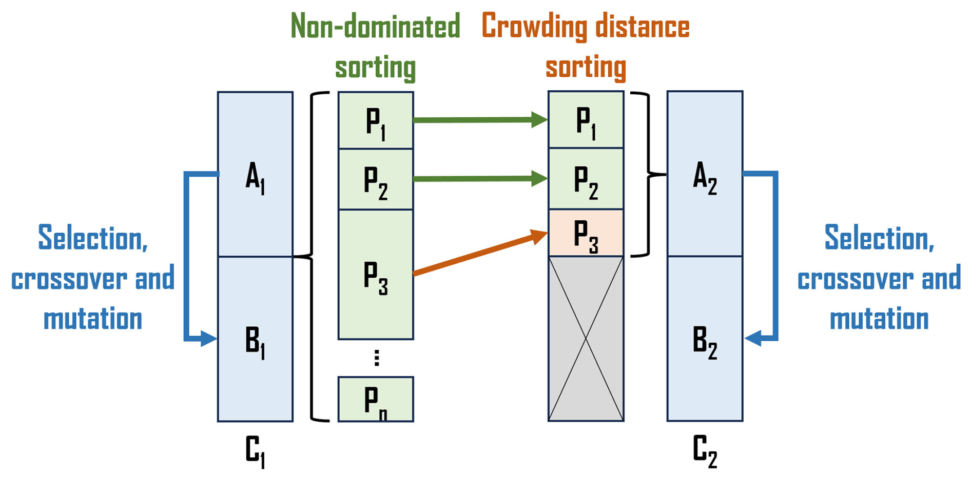
Figure 2 Brief workflow of NSGA-II (A: the parent population; B: the offspring population; C: the new population; P: the Pareto front).

The workflow of NSGA-II is summarized as follows (Fig. 2).

• a.

  Randomly generating an initial population (A₁) of size N. Performing selection, crossover and mutation operations on A₁ to generate an offspring population (B₁) of size N. The parent population (A₁) and the offspring population (B₁) are combined to form a new population (C₁) of size 2N.

• b.

  Performing a rapid non-dominated sorting on C₁ to generate the Pareto fronts (P_i, $i=\mathrm{1},\mathrm{2},\mathrm{\dots },n$) at different ranks.

• c.

  Filling the next population (A₂) of size N with P_i based on the rank order.

• d.

  When A₂ is filled to the point of insufficient capacity to contain the entire P_i, the optimal solutions in P_i are inserted into A₂ in a priority order identified by the non-dominated sorting and crowding distance until the size of A₂ reaches N.

• e.

  Performing selection, crossover and mutation operations on A₂ to generate an offspring population (B₂) of size N. The parent population (A₂) and offspring population (B₂) combine to form a new population (C₂) of size 2N.

• f.

  Iterating steps (b) to (e) until the convergence criteria are satisfied.

2.2.4 Framework training and evaluation

An hourly multivariate dataset with extensive temporal coverage was employed to train and evaluate the deep learning module. To maintain temporal independence, the training (and validation) set was constructed from a 1-year (2021) time-series dataset obtained from a Beijing site (Fig. S1), while the testing set contains an independent 6-month (1 January–31 March and 1 June to 31 August 2022) time-series dataset obtained from the same site. A 10-fold time-series cross-validation (CV) scheme was designed for the training (and validation) set to preserve its temporal order and prevent future information leakage, which is detailed in Sect. S3 and Fig. S2 in the Supplement. The iteration number of Bayesian optimization is set to 20.

To fully evaluate the performance of the retrieval framework in predicting vertical profiles of NH${}_{\mathrm{4}}^{+}$, SO${}_{\mathrm{4}}^{\mathrm{2}-}$, NO${}_{\mathrm{3}}^{-}$, OM and BC, we conduct three retrieval experiments: (1) We compare the retrieved mass concentrations with the observed values at the surface level during a training year (2021) and three non-training years (2017, 2018 and 2024) to validate the temporal generalization in all seasons and under diverse meteorological conditions. (2) We assess the spatial generalization ability by applying the retrieval framework to 23 non-training lidar sites in the NCP from 8–15 February 2021 and comparing the retrieved mass concentrations with observations at the surface level. The spatial distribution of the 23 non-training lidar sites is presented in Fig. S1. (3) We validate the retrieved vertical profiles by aircraft-based and tower-based vertical observations during several non-training episodes. Subsequently, SHapley Additive exPlanations (SHAP), a local explainable technology (Lundberg et al., 2020), has been widely employed in prediction interpretation for varying machine learning models (Li et al., 2025b; Hou et al., 2022), is integrated into the deep learning module to quantify the impact of multivariate input features on the retrieval of PM_2.5 chemical components. Finally, we applied this retrieval framework to generate a long-term vertical profile dataset for five PM_2.5 chemical components in a megacity over six years of 2017–2018 and 2021–2024.

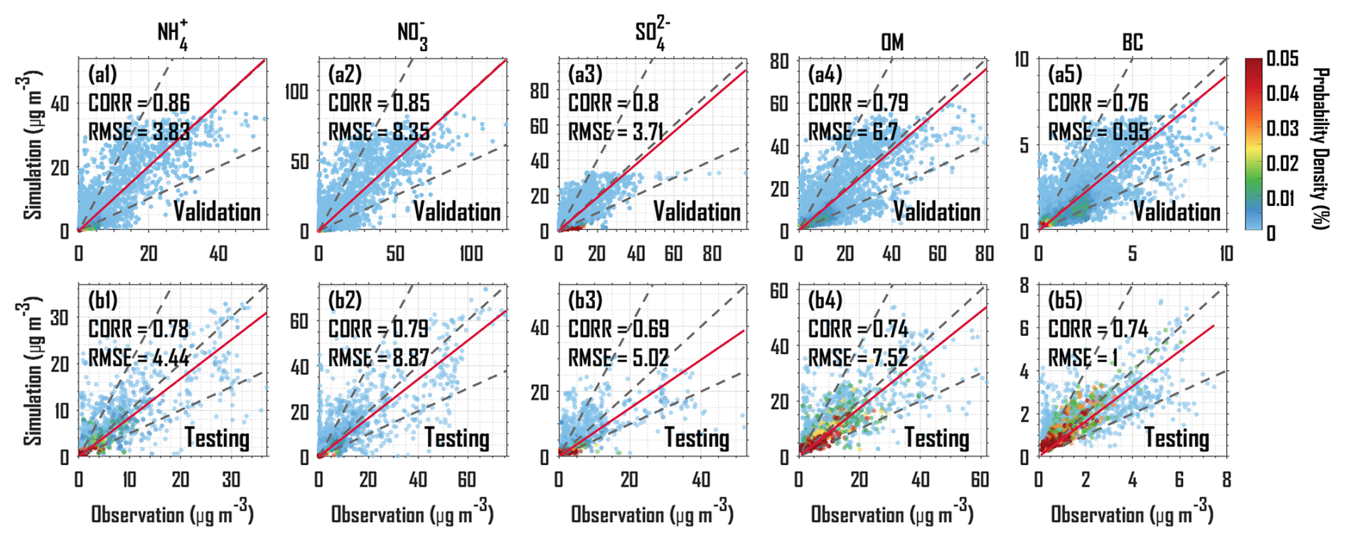
Figure 3 Scatterplots of the simulations (µg m⁻³) versus the observations (µg m⁻³) with probability density (%) for NH${}_{\mathrm{4}}^{+}$, NO${}_{\mathrm{3}}^{-}$, SO${}_{\mathrm{4}}^{\mathrm{2}-}$, OM and BC during the 10-fold cross-validation process (a1–a5) and temporally independent testing process (b1–b5). The dotted grey lines represent the 2:1, 1:1, and 1:2 lines, and the solid red line represents the fitted regression line. CORR represents the correlation coefficient, and RMSE represents root mean square error.

3 Results and discussion

3.1 Validation

3.1.1 Evaluation of the deep learning module performance

The 10-fold CV sets and a testing set with temporal independence are utilized to evaluate the predictive performance of the deep learning module, which is quantified by the discrepancies between simulations and observations at ground level for NH${}_{\mathrm{4}}^{+}$, SO${}_{\mathrm{4}}^{\mathrm{2}-}$, NO${}_{\mathrm{3}}^{-}$, OM and BC. Overall, the scatter distribution and fitted regression line closely align with the 1:1 line in both the 10-fold CV (Fig. 3a1–a5) and temporally independent testing phases (Fig. 3b1–b5). The error distributions are concentrated around 0, with mean errors between $-\mathrm{1.78}\pm \mathrm{8.15}$ and $-\mathrm{0.13}\pm \mathrm{0.94}$ µg m⁻³ during the 10-fold CV phase (Fig. S3a1–a5) and between $-\mathrm{1.36}\pm \mathrm{7.40}$ and $-\mathrm{0.07}\pm \mathrm{1.00}$ µg m⁻³ during the temporally independent testing phase (Fig. S3b1–b5), demonstrating strong consistency between observations and simulations. Notably, the error distributions for the validation and independent testing sets are closely aligned, indicating that the deep learning module is robust and generalizes well to unseen data. Specifically for the 10-fold CV process (Fig. 3a1–a5), the CORR values for the five PM_2.5 chemical components range from 0.76 to 0.86, indicating that the deep learning module accurately interprets the relationship between multivariate input features and the five PM_2.5 chemical components. The RMSE values range from 0.95 to 8.35 µg m⁻³, indicating a low discrepancy between simulations and observations. Compared to the 10-fold CV process, the temporally independent testing yields slightly lower CORR values (0.69–0.79) and higher RMSE values (1.00–8.87 µg m⁻³), showing a slight underestimation for the five PM_2.5 chemical components (Fig. 3b1–b5). It is expected that the statistical results from the temporally independent testing are less robust than those from the 10-fold CV, since the temporally independent testing set aggregates a broader spectrum of temporal patterns compared to the validation set at each fold. Our statistical results from the 10-fold CV exhibit similarities or even improvements compared to those reported in other studies that predicting PM_2.5 chemical component concentrations based on machine learning models (Lv et al., 2021; Lin et al., 2022; Araki et al., 2022; Liu et al., 2023), indicating that the deep learning module demonstrates strong prediction capabilities.

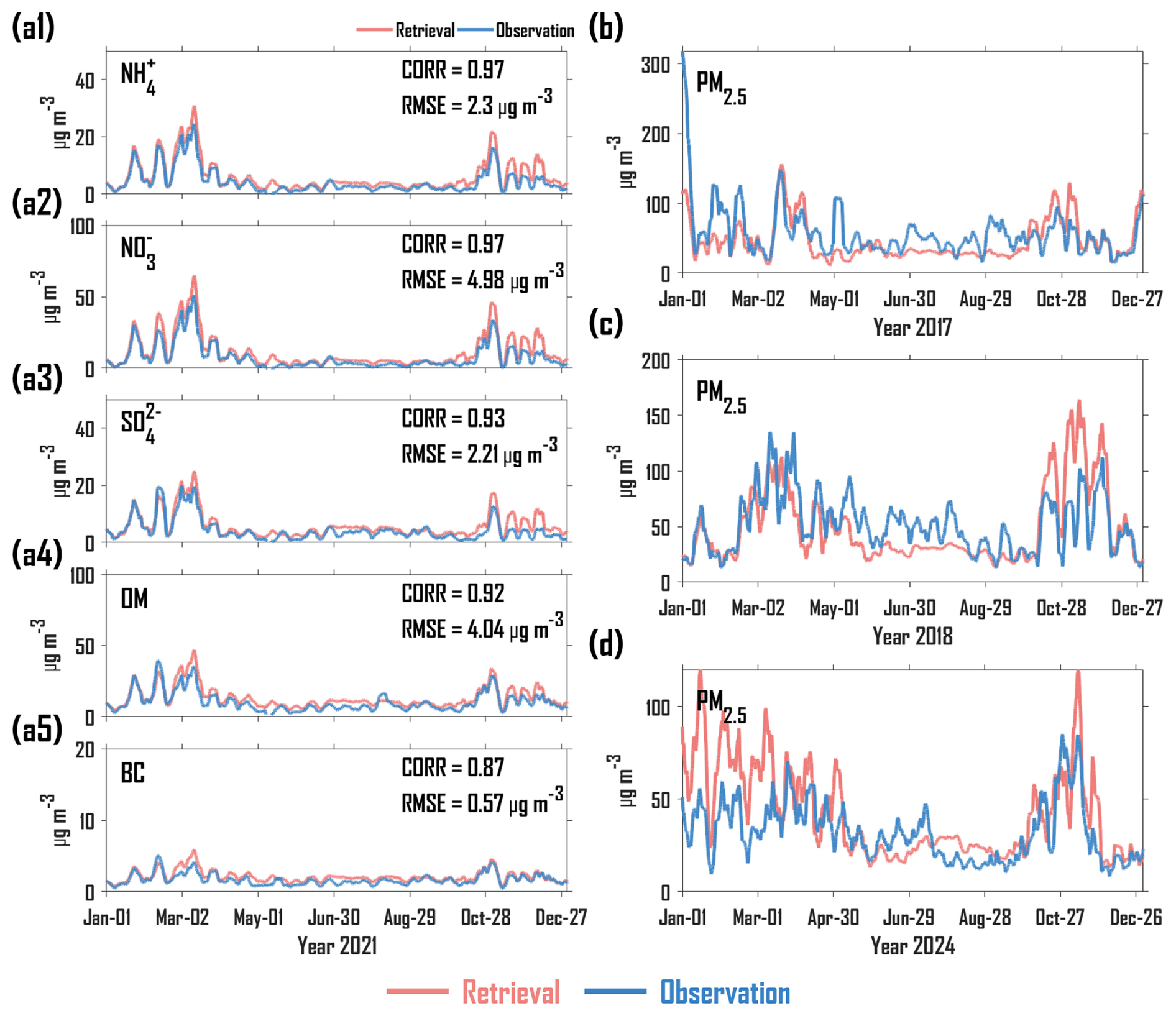
Figure 4 Weekly-smoothed variations in the retrieved and observed concentrations (µg m⁻³) of NH${}_{\mathrm{4}}^{+}$ (a1), NO${}_{\mathrm{3}}^{-}$ (a2), SO${}_{\mathrm{4}}^{\mathrm{2}-}$ (a3), OM (a4) and BC (a5) in 2021. (b) same as (a1)–(a5) but for PM_2.5 in 2017. (c) same as (a1)–(a5) but for PM_2.5 in 2018. (d) same as (a1)–(a5) but for PM_2.5 in 2024. CORR represents the correlation coefficient, RMSE represents root mean square error.

3.1.2 Comparison with ground-level observations

The retrieval framework was applied to retrieve the vertical profiles of NH${}_{\mathrm{4}}^{+}$, NO${}_{\mathrm{3}}^{-}$, SO${}_{\mathrm{4}}^{\mathrm{2}-}$, OM and BC in a Beijing lidar site (39.98° N, 116.38° E) over a training year (2021) and three non-training years (2017, 2018 and 2024). As illustrated in Fig. 4a1–a5, the weekly-smoothed variations in the retrieved surface concentrations of the five PM_2.5 chemical components demonstrate strong consistency with the observed surface concentrations for the training year, indicating that the retrieval framework adequately captures the temporal characteristics of these chemical components. The CORR values between the retrieved and observed concentrations range from 0.87 to 0.97, surpassing those of the deep learning module (Figs. 4a1–a5 and 3b1–b5). In addition, the RMSE values for all five chemical components (0.57–4.98µg m⁻³) are consistently lower than those from the deep-learning module (Figs. 4a1–a5 and 3b1–b5). These results demonstrate that the physics-constrained optimization effectively enhances the retrieval accuracy of chemical component concentrations.

For the non-training years, the retrieved surface concentrations of a sum of five PM_2.5 chemical components are compared to the observed surface PM_2.5 concentrations, owing to the absence of long-term observations for individual chemical components. As shown in Fig. 4b–d, the weekly-smoothed variations in the retrieved surface PM_2.5 concentrations closely align with the observed values in 2017, 2018 and 2024. The high values of surface PM_2.5 concentration observed in March–April and November of 2018 and 2024 are effectively captured by the retrieval framework. These results indicate that the retrieval framework roughly interprets the changes in concentrations of various chemical components across different periods, exhibiting fundamental temporal generalization capabilities. However, the retrieved concentrations show some overestimation cases during autumn in 2018 and spring in 2024, potentially associated with the uncertainties induced by the training data. The training data may lack a sufficiently diverse spectrum of meteorological conditions and pollution patterns, which limits the temporal generalizability of the retrieval framework across all complex and dynamic atmospheric scenarios. Future efforts should enhance retrieval accuracy by augmenting the training data with observations spanning a wider range of temporal conditions.

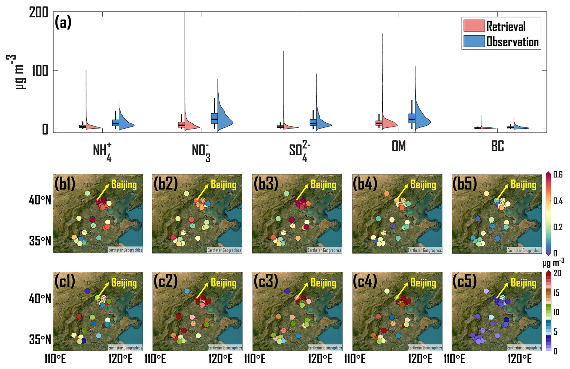
Figure 5 Data distribution properties of retrieved and observed surface mass concentration (µg m⁻³) of NH${}_{\mathrm{4}}^{+}$, NO${}_{\mathrm{3}}^{-}$, SO${}_{\mathrm{4}}^{\mathrm{2}-}$, OM and BC at 23 non-training NCP lidar sites over a period of 8–15 February 2021, presented by a combination of boxplots and kernel density (a). Spatial distribution of Pearson correlation coefficient (CORR) between retrieved and observed surface mass concentration of NH${}_{\mathrm{4}}^{+}$ (b1), NO${}_{\mathrm{3}}^{-}$ (b2), SO${}_{\mathrm{4}}^{\mathrm{2}-}$ (b3), OM (b4) and BC (b5). (c1)–(c5) Same as (b1)–(b5) but for root mean square error (RMSE, µg m⁻³). The geographic basemap is hosted by Esri | Powered by Esri (https://www.esri.com/en-us/home, last access: 8 January 2026).

The retrieval framework was also applied to retrieve the vertical profiles of the five PM_2.5 chemical components at 23 non-training NCP lidar sites over a short-term period of 8–15 February 2021, aiming to validate its spatial generalization capabilities. Compared with the observed surface concentrations at 23 non-training sites, the retrieved surface concentrations exhibit a more clustered data distribution and exhibit a tendency toward underestimation across all components (Fig. 5a). The site-averaged CORR values for the five chemical components range from 0.21 to 0.46, with RMSE values spanning 2.7 to 20.37 µg m⁻³ (Fig. S4). From a spatial perspective (Fig. 5b1–b5), non-training NCP sites located closer to the Beijing lidar site exhibit higher CORR values, with the highest reaching 0.71 (NH${}_{\mathrm{4}}^{+}$), 0.56 (NO${}_{\mathrm{3}}^{-}$), 0.81 (SO${}_{\mathrm{4}}^{\mathrm{2}-}$), 0.48 (OM) and 0.41 (BC). Conversely, the RMSE values are not affected by the distance from the Beijing lidar site (Fig. 5c1–c5), with the lowest reaching 2.91 µg m⁻³ (NH${}_{\mathrm{4}}^{+}$), 6.15 µg m⁻³ (NO${}_{\mathrm{3}}^{-}$), 3.05 µg m⁻³ (SO${}_{\mathrm{4}}^{\mathrm{2}-})$, 6.59 µg m⁻³ (OM) and 0.78 µg m⁻³ (BC). However, several sites exhibit poor retrieval performance, with CORR values ranging from ∼0.20 to ∼0.30 (Fig. S5), which is primarily attributed to limitations in the spatial representativeness of the training data. The deep-learning module was trained exclusively on a long-term dataset from a single site in Beijing, which is insufficient to capture the spatial variability in emission intensity, as well as local meteorological and geographical conditions across the broader NCP. As a result, the spatial extrapolation capability of the deep-learning module is constrained. Although the retrieval framework can retrieve PM_2.5 chemical component concentrations at spatially distributed lidar sites, future work should incorporate long-term datasets from varying locations to enhance spatial generalization and extrapolation performance.

Figure 6 Vertical profiles (µg m⁻³) of NH${}_{\mathrm{4}}^{+}$, NO${}_{\mathrm{3}}^{-}$, SO${}_{\mathrm{4}}^{\mathrm{2}-}$, and OM from retrieval (a1) and tower-based observation (a2) during a period from 30 December 2018 to 2 January 2019 in Beijing. The line represents the daily average of the hourly vertical profiles, and the shaded area represents the standard deviation. Averaged proportions of NH${}_{\mathrm{4}}^{+}$, NO${}_{\mathrm{3}}^{-}$, SO${}_{\mathrm{4}}^{\mathrm{2}-}$, OM, and BC from retrieval (b1) and tower-based observation (b2) for 10 d (27 and 30 December 2023; 2, 5, 9, 12, 15, 18, 24, and 27 January 2024). (c1) and (c2) Same as (b1) and (b2) but for aircraft-based verification for 3 d (26 September, 10 October, 11 December 2024).

3.1.3 Verification of retrieved vertical profiles

In addition to the spatiotemporal verification of surface-level mass concentrations, tower-based and aircraft-based observational experiments were conducted to validate the retrieved vertical profiles of five PM_2.5 chemical components during non-training periods. From the surface to ∼200 m altitude, the retrieved and observed vertical profiles exhibit similar vertical patterns during a period from 30 December 2018 to 2 January 2019 in Beijing, with higher concentrations occurring at altitudes of 50–80 m for NH${}_{\mathrm{4}}^{+}$, NO${}_{\mathrm{3}}^{-}$, SO${}_{\mathrm{4}}^{\mathrm{2}-}$ and OM (Fig. 6a1, a2). Specifically, as presented in Table S3, the CORR values are no less than 0.66 for all four PM_2.5 chemical components. However, the RMSE value for OM (23.04 µg m⁻³) is notably higher than that for the other components (4.08–10.48 µg m⁻³), indicating limitations in the retrieval framework when representing the vertical profile of OM during winter pollution episodes. This discrepancy may be associated with retrieval uncertainties arising from input data quality and imposed physical constraints. Additionally, the retrieved and observed proportions of NH${}_{\mathrm{4}}^{+}$, NO${}_{\mathrm{3}}^{-}$, SO${}_{\mathrm{4}}^{\mathrm{2}-}$, OM and BC demonstrate significant consistency (Fig. 6b1, b2). Among these chemical components, NO${}_{\mathrm{3}}^{-}$ and OM contribute the largest proportions, followed by NH${}_{\mathrm{4}}^{+}$ and SO${}_{\mathrm{4}}^{\mathrm{2}-}$, while BC contributes the smallest fraction. This proportional characteristic is evident in both the retrieved and observed proportions at altitudes of 600 and 1200 m (Fig. 6c1, c2). Due to the lack of NH${}_{\mathrm{4}}^{+}$ measurements at 1500 m and the absence of both NH${}_{\mathrm{4}}^{+}$ and SO${}_{\mathrm{4}}^{\mathrm{2}-}$ measurements at 2100 m, the proportions at these altitudes are statistically inferred from the remaining chemical components. The results indicate overall consistency between retrieved and observed proportions at altitudes of 1500 and 2100 m, although the proportion of NO${}_{\mathrm{3}}^{-}$ is slightly overestimated at 2100 m and underestimated at 1500 m. Overall, the tower-based and aircraft-based verifications indicate that the retrieval framework achieves high accuracy in retrieving the vertical profiles of the five PM_2.5 chemical components during non-training period, demonstrating its robust generalization capability and reliability when applied to independent datasets.

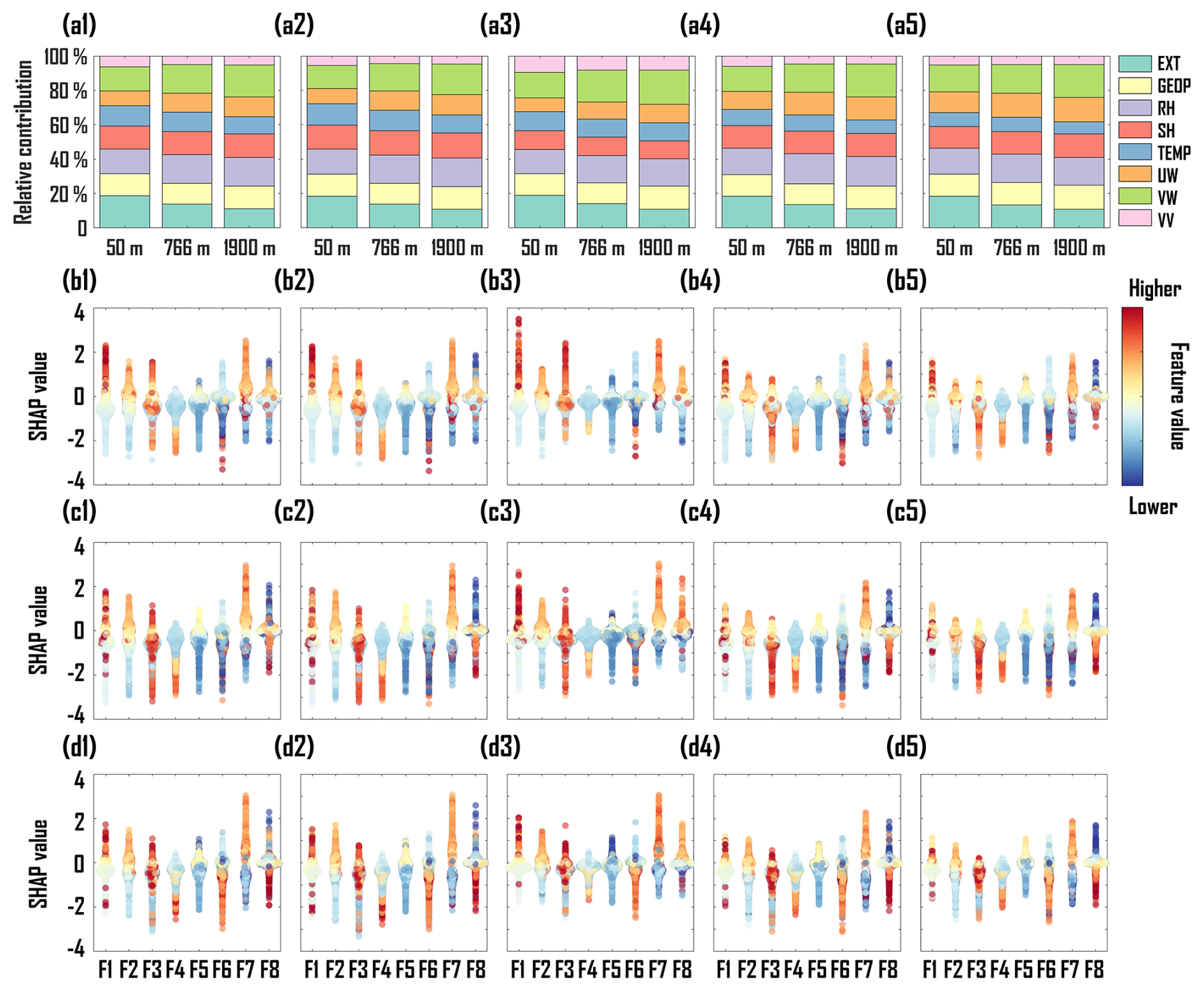
Figure 7 Relative contribution of 8 input features on predictive NH${}_{\mathrm{4}}^{+}$ (a1), NO${}_{\mathrm{3}}^{-}$ (a2), SO${}_{\mathrm{4}}^{\mathrm{2}-}$ (a3), OM (a4) and BC (a5) at altitudes of 50, 766 and 1900 m. SHAP values with feature values of 8 input features for predictive NH${}_{\mathrm{4}}^{+}$ (b1), NO${}_{\mathrm{3}}^{-}$ (b2), SO${}_{\mathrm{4}}^{\mathrm{2}-}$ (b3), OM (b4) and BC (b5) at an altitude of 50 m. (c1)–(c5) Same as (b1)–(b5) but for an altitude of 766 m. (d1)–(d5) Same as (b1)–(b5) but for an altitude of 1900 m. F1: extinction coefficient at 532 nm, EXT; F2: Geopotential, GEOP; F3: Relative humidity, RH; F4: Specific humidity, SH; F5: Temperature, TEMP; F6: U-component wind, UW; F7: V-component wind; F8: Vertical velocity, VV.

3.2 Assessment of feature importance

The predictive performance of the deep learning module is intricately connected to the input features (Blum and Langley, 1997). Although the module incorporates the CNN and attention mechanism layer to mitigate issues related to feature dimension, the impact of input features on the module predictions remains ambiguous, which impedes module interpretability and restricts the capacity to enhance the module performance through effective feature selection. The SHAP method is employed to quantify the relative contributions of 8 input features to the predictions of the five PM_2.5 chemical components at various heights and to identify the impact of the input features on the decision-making processes of the deep learning module. The coexistence of a high feature value with a positive SHAP value in a specific feature implies an amplification of concentration prediction at elevated levels.

Figure 7a1–a5 depicts that the aerosol extinction coefficient at 532 nm (EXT), relative humidity (RH) and v-component wind (VW) are the significant input features for predicting the five PM_2.5 chemical components with an averaged relative contribution of 14.43 %, 15.84 % and 16.77 %. These features largely affect the vertical structure, chemical and physical processes, respectively. Specifically, EXT characterizes the vertical distribution of a total of the five PM_2.5 chemical components and plays a crucial indicative role in vertical profile predictions (Tao et al., 2016). RH is a key driving factor in aerosol hygroscopic growth, aqueous-phase chemical reactions, and heterogeneous reactions, significantly contributing to the mass concentrations of varying chemical components as reported in numerous studies (Fang et al., 2019; Wang et al., 2020; Gao et al., 2020; Liang et al., 2019). VW primarily affects latitudinal transboundary transport, which is a dynamic forcing in the southwest-northeast transport channel of the Beijing-Tianjin-Hebei (BTH) region (Yang et al., 2024). Notably, the relative contribution of EXT decreases with height from the surface (50 m) to the free atmosphere (1900 m), while the relative contribution of VW exhibits an opposite trend. The aerosol content in the upper planetary boundary layer is relatively low, and the weakened lidar aerosol signal is susceptible to interference from noise signals, restricting the indicative effect of EXT on chemical component concentrations. Conversely, pollution transport in the upper planetary boundary layer is less affected by interference from complex underlying surfaces than near-surface transport (Wu et al., 2019b), amplifying the driving effect of high-altitude VW on chemical component concentrations. Specific humidity (SH) and geopotential (GEOP) also provided important contributions (13.04 % and 12.85 %, respectively). SH is related to the vertical diffusion and wet scavenging of pollutants (Chatfield et al., 2020) and GEOP identifies the synoptic meteorological patterns that affect both horizontal process (Jia et al., 2022; Wang et al., 2021) and vertical distribution of pollutants within the boundary layer (Miao et al., 2022; Xu et al., 2019).

Figure 7b1–d5 further determines the impact of the input features on the decision-making processes of the deep learning module. From Fig. 7b1–b5, the elevated levels of EXT, GEOP, and VW significantly enhance the concentration predictions of the five PM_2.5 chemical components in the near-surface layer (50 m), while high-level RH exert either positive or negative effects on predictions. High RH not only facilitates aqueous-phase and heterogeneous chemical reactions, positively contributing to predictions, but also promotes aerosol coalescence, leading to dry and wet deposition that negatively contributes to predictions (Chen et al., 2020). The results in the middle of the boundary layer (766 m) are consistent with those observed in the near-surface layer (Fig. 7c1–c5). Particularly, the positive driving effect of lower VV values on predictions is more significant, with downward wind contributing positively to predictions, which is attributed to the fact that sinking airflows inhibit the dispersion of chemical components, thereby exacerbating aggregation and increasing concentration (Yang et al., 2022). The results in the free atmosphere (1900 m) align with those in the middle of the boundary layer (Fig. 7d1–d5). Notably, the influence of UW on predictions is more apparent, as the westerly wind positively contributes to the predictions, which is primarily due to the elevated emission sources located in the southwestern BTH region (Yang et al., 2024). Strong prevailing southwesterly winds at high altitudes enhance the regional transport of atmospheric pollutants, leading to an increase in concentration.

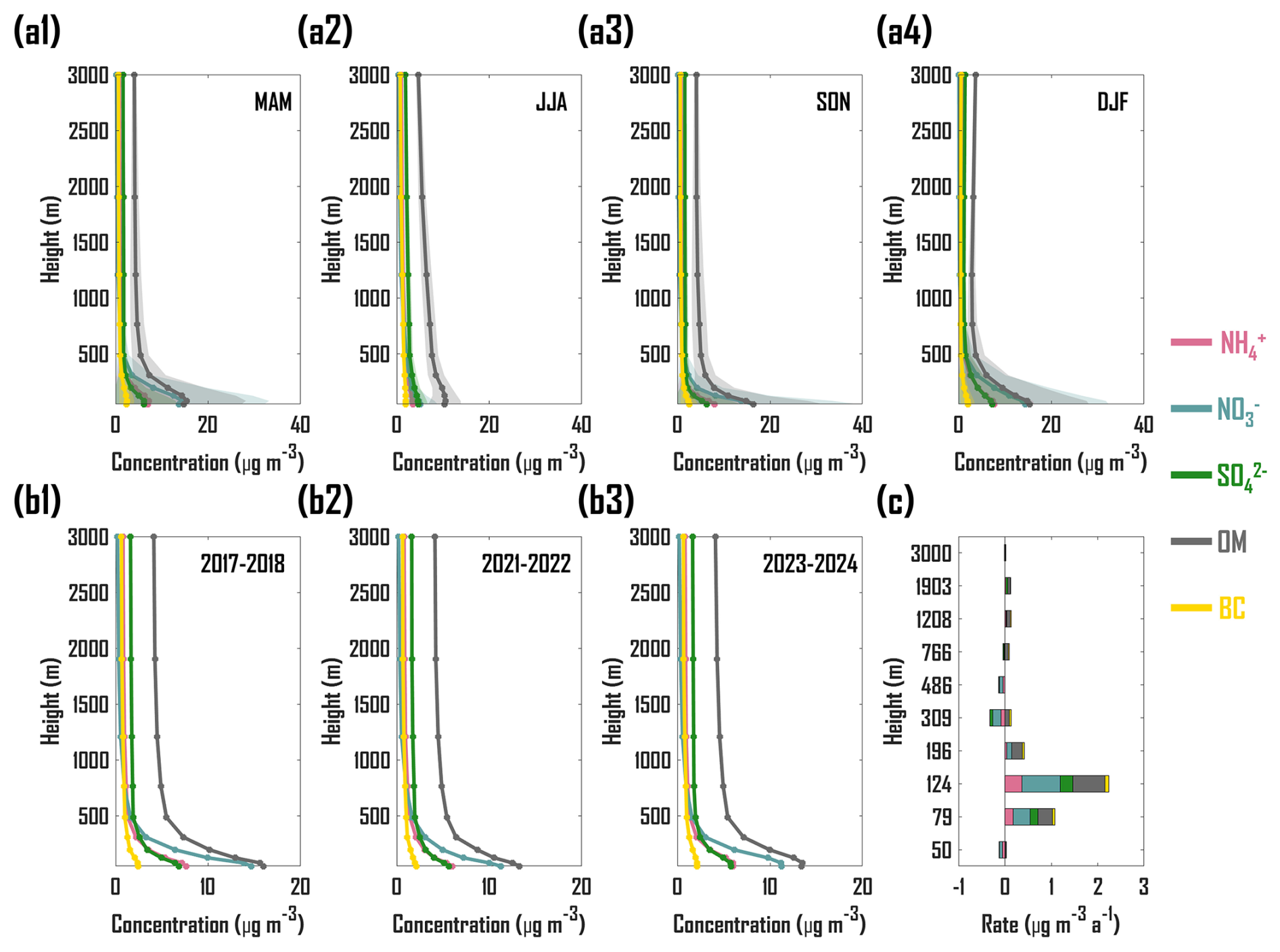
Figure 8 Vertical distribution of mass concentrations (µg m⁻³) for NH${}_{\mathrm{4}}^{+}$, NO${}_{\mathrm{3}}^{-}$, SO${}_{\mathrm{4}}^{\mathrm{2}-}$, OM and BC in spring (MAM, a1), summer (JJA, a2), autumn (SON, a3) and winter (DJF, a4) over six years (2017–2018, 2021–2024). Averaged vertical profiles of mass concentrations (µg m⁻³) for NH${}_{\mathrm{4}}^{+}$, NO${}_{\mathrm{3}}^{-}$, SO${}_{\mathrm{4}}^{\mathrm{2}-}$, OM and BC from 2017 to 2018 (b1), from 2021 to 2022 (b2), and from 2023 to 2024 (b3). Annual change rates (µg m⁻³ a⁻¹) of mass concentrations for NH${}_{\mathrm{4}}^{+}$, NO${}_{\mathrm{3}}^{-}$, SO${}_{\mathrm{4}}^{\mathrm{2}-}$, OM and BC at various altitudes from 2021 to 2024 (c).

3.3 Application of the retrieval framework

The retrieval framework was applied to generate a long-term dataset of vertical profiles for NH${}_{\mathrm{4}}^{+}$, NO${}_{\mathrm{3}}^{-}$, SO${}_{\mathrm{4}}^{\mathrm{2}-}$, OM and BC over six years (2017–2018, 2021–2024) at a Beijing lidar site. Figure 8 shows the averaged vertical profiles for the five PM_2.5 chemical components in spring (MAM) (Fig. 8a1), summer (JJA) (Fig. 8a2), autumn (SON) (Fig. 8a3) and winter (DJF) (Fig. 8a4) during the six years. OM mass concentrations are consistently the highest across all four seasons, followed by NO${}_{\mathrm{3}}^{-}$, while the mass concentrations of NH${}_{\mathrm{4}}^{+}$, SO${}_{\mathrm{4}}^{\mathrm{2}-}$ and BC remain relatively low. The high proportions of OM and NO${}_{\mathrm{3}}^{-}$ in Chinese PM_2.5 pollution were frequently reported in recent studies (Zhang et al., 2024; Liu et al., 2022). Since the implementation of the Air Pollution Prevention and Control Action Plan during 2013–2017 and the Three-year Action Plan to Win the Blue-Sky Defense War during 2018–2020 in China, effective reductions in sulfur dioxide (SO₂) have gradually shifted the dominated chemical component of PM_2.5 pollution from SO${}_{\mathrm{4}}^{\mathrm{2}-}$ to OM and NO${}_{\mathrm{3}}^{-}$ (Niu et al., 2022). Furthermore, the decreased SO${}_{\mathrm{4}}^{\mathrm{2}-}$ mass concentrations have amplified the competitive effect of NO${}_{\mathrm{3}}^{-}$ on capturing NH₃ and NH${}_{\mathrm{4}}^{+}$ in the thermodynamic equilibrium process, increasing NO${}_{\mathrm{3}}^{-}$ mass concentrations (Geng et al., 2024). In comparison to the mass concentrations of the five PM_2.5 chemical components in MAM, SON and DJF, summertime mass concentrations are notably lower, which are attributed to reduced heating activities and enhanced wet deposition during summer periods (Liu et al., 2015; Ji et al., 2019). Moreover, the summertime vertical distributions of the five chemical components are relatively uniform, which may be attributed to the enhanced atmospheric vertical mixing effects induced by the unstable boundary layer (Roostaei et al., 2024).

Figure 8 also shows the averaged vertical profiles for 2017–2018 (Fig. 8b1), 2021–2022 (Fig. 8b2) and 2023–2024 (Fig. 8b3), as well as the annual change rate during 2021–2024 in Beijing (Fig. 8c). During 2017–2018, the implementation of clean air policies resulted in mass concentrations of NH${}_{\mathrm{4}}^{+}$, SO${}_{\mathrm{4}}^{\mathrm{2}-}$ and BC remaining below 8 µg m⁻³ (Fig. 8b1). However, the mass concentrations of NO${}_{\mathrm{3}}^{-}$ exceeded 13 µg m⁻³ at altitudes below ∼125 m, and those of OM exceeded 15 µg m⁻³ below ∼100 m, likely due to the nonlinear response to emission reduction (Li et al., 2021). Compared to 2017–2018, the mass concentrations of NH${}_{\mathrm{4}}^{+}$, NO${}_{\mathrm{3}}^{-}$, SO${}_{\mathrm{4}}^{\mathrm{2}-}$, OM and BC decreased significantly during 2021–2022 with average reductions of 8.36 %, 10.65 %, 6.58 %, 8.58 % and 5.85 %, respectively, from 50 to 3000 m (Fig. 8b2). These decreases are attributed to the continued implementation of clean air policies and reduced emissions associated with the COVID-19 pandemic control in China (Kang et al., 2020). During 2023–2024, the mass concentrations of NH${}_{\mathrm{4}}^{+}$, NO${}_{\mathrm{3}}^{-}$, SO${}_{\mathrm{4}}^{\mathrm{2}-}$, OM and BC increased relative to the 2021–2022 levels, with average increases of 5.49 %, 6.43 %, 4.65 %, 5.75 % and 4.40 %, respectively, from 50 to 3000 m (Fig. 8b3). This rebound over the NCP has be reported previously and is likely related to the offsetting effect of enhanced human activities following the relaxation of the COVID-19 pandemic lockdowns on the implementation of clean air policies (Song et al., 2025). From 2021 to 2024, the change rates of NH${}_{\mathrm{4}}^{+}$, NO${}_{\mathrm{3}}^{-}$ and SO${}_{\mathrm{4}}^{\mathrm{2}-}$ at approximately 50, 310 and 770 m exhibit decreasing trends, with decrease rates ranging from 0.06 to 0.19 µg m⁻³ a⁻¹. In contrast, the change rates of the five chemical components at approximately 80, 120, 1210 and 1900 m show increasing trends, with the highest increase rate of 0.83 µg m⁻³ a⁻¹ occurring at ∼120 m for NO${}_{\mathrm{3}}^{-}$ (Fig. 8c). In addition, OM exhibited a significant increase rate of 0.69 µg m⁻³ a⁻¹ at ∼120 m, which may be related to the low sensitivity of high-altitude organic aerosols to emission controls (Zhao et al., 2017). Future clean air policies should prioritize strengthening control measures for OM and NO${}_{\mathrm{3}}^{-}$ within the lower and middle parts of the atmospheric boundary layer.

3.4 Limitations and uncertainties

The deep learning module in our retrieval framework can establish a powerful mapping between optical and meteorological features and PM_2.5 chemical species, and physics-based explicit constraints can enhance the reliability and expandability of the mapping relationships. However, several limitations and sources of uncertainty remain and should be acknowledged when interpreting the results and extending the framework to broader applications.

First, the spatial scope of the training data is predominantly restricted to the NCP region. Expanding the retrieval framework with data from more diverse geographical locations is necessary to improve its global transferability. Second, the current retrieval framework primarily relies on extinction coefficients at a wavelength of 532 nm, exhibiting dependence on specific lidar instruments. Future retrieval framework should focus on integrating diverse optical features from additional wavelengths to enhancing adaptability and transferability. Third, the auxiliary input data used in both the deep learning module and the physics-constrained optimization are obtained from global reanalysis products, which may not fully capture local atmospheric conditions at specific observational sites, thereby introducing representativeness errors into the retrievals. Acquiring the vertical observational data for these auxiliary features can effectively mitigate the uncertainty induced by the input data. Fourth, the IMPROVE equation applied as an external physical constraint may introduce additional uncertainty into the retrievals due to its systematic estimation biases (Lowenthal and Kumar, 2016). Moreover, since the IMPROVE equation was applied as an external physical constraint to optimize the retrievals of PM_2.5 chemical components, the machine learning model itself was not intrinsically constrained by physical principles during its training. Future work could incorporate an internal physical constraint into the machine learning model to improve its physical interpretability by formulating a hybrid loss function for training that combines the traditional data-fitting term with a physical term. Finally, long-term acquisition of independent vertical profiling data from both tower-based and aircraft-based campaigns is essential for a comprehensive assessment of the robustness of the vertical retrievals with respect to varying sites, aerosol types, and seasons.

4 Conclusions

This study proposes a novel lidar-based retrieval framework for obtaining the vertical profiles of five PM_2.5 chemical components (NH${}_{\mathrm{4}}^{+}$, SO${}_{\mathrm{4}}^{\mathrm{2}-}$, NO${}_{\mathrm{3}}^{-}$, OM and BC) for the first time. A long-term multivariate dataset was utilized to train a complex deep-learning module in the retrieval framework, thus interpreting the nonlinear relationship among lidar parameters, meteorological parameters and PM_2.5 chemical components. A physics-constrained optimization module was integrated into the retrieval framework, enhancing the generalization capabilities of predicting vertical profiles across diverse spatiotemporal scenarios.

In situ surface observations of hourly mass concentrations of PM_2.5 and its five chemical components over a training year and three non-training years were used to validate the accuracy of the retrieval framework in interpreting temporal variations. The results showed that the Pearson correlation coefficient values between the retrieved and observed concentrations ranged from 0.87 to 0.97 during the training year, and the variations in the retrieved surface PM_2.5 mass concentrations closely aligned with the observations during the non-training year, indicating the robust capabilities of temporal prediction and generalization in the retrieval framework. The retrieval framework was then applied to obtain the mass concentrations of five PM_2.5 chemical components at 23 non-training sites. The retrieved results exhibited patterns that are moderately consistent with the corresponding observations. However, limitations remained in accurately capturing short-term temporal variations, with a general tendency toward underestimation. Tower-based and aircraft-based field campaigns at altitudes ranging from surface to 2100 m were conducted to validate the accuracy of the retrieved vertical profiles of NH${}_{\mathrm{4}}^{+}$, SO${}_{\mathrm{4}}^{\mathrm{2}-}$, NO${}_{\mathrm{3}}^{-}$, OM and BC. The tower-based and aircraft-based verifications indicate that the retrieved and observed vertical profiles of these components exhibited consistent patterns in mass concentrations and proportions, demonstrating the robust capabilities of the retrieval framework in obtaining high-precision vertical profiles from non-training datasets. Subsequently, SHapley Additive exPlanations (SHAP), an explainable technology, is integrated into the deep learning module to quantify the impact of multivariate input features on the retrieval of PM_2.5 chemical components. The results showed that the aerosol extinction coefficient at 532 nm, relative humidity and v-component wind are the dominant input features for predicting the five PM_2.5 chemical components with an averaged relative contribution of 14.43 %, 15.84 % and 16.77,%. The driving effect of the input features on the decision-making processes of the deep learning module was also determined by SHAP values.

Finally, we applied this framework to generate a long-term dataset of vertical profiles for NH${}_{\mathrm{4}}^{+}$, SO${}_{\mathrm{4}}^{\mathrm{2}-}$, NO${}_{\mathrm{3}}^{-}$, OM and BC over six years (2017–2018, 2021–2024). From this dataset, we found that OM mass concentrations are consistently the highest across all four seasons, followed by NO${}_{\mathrm{3}}^{-}$, while the mass concentrations of NH${}_{\mathrm{4}}^{+}$, SO${}_{\mathrm{4}}^{\mathrm{2}-}$ and BC remain relatively low. From 2021 to 2024, the change rates of NH${}_{\mathrm{4}}^{+}$, NO${}_{\mathrm{3}}^{-}$ and SO${}_{\mathrm{4}}^{\mathrm{2}-}$ at approximately 50, 310 and 770 m exhibit decreasing trends, with decrease rates ranging from 0.06 to 0.19 µg m⁻³ a⁻¹. However, OM and NO${}_{\mathrm{3}}^{-}$ exhibited significant increase rates of 0.69 and 0.83 µg m⁻³ a⁻¹, respectively, at an altitude of ∼120 m. Future clean air policies should prioritize strengthening control measures for OM and NO${}_{\mathrm{3}}^{-}$ within the lower and middle parts of the atmospheric boundary layer. Our new retrieval framework offers a novel approach to acquiring vertical profiles of PM_2.5 chemical components. Future efforts should aim to mitigate the overestimation of carbonaceous aerosols by regulating the parameters involved in the physics-constrained optimization process.