Laminar gas inlet – Part 2: Wind tunnel chemical transmission measurement and modelling

Aircraft-based measurements of gas-phase species and aerosols provide crucial knowledge about the composition and vertical structure of the atmosphere, enhancing the study of atmospheric physics and chemistry. Unlike aircraft-based aerosol particle sampling systems, the gas loss mechanisms and transmission efficiency of aircraft-based gas sampling systems are rarely discussed. In particular, the gas transmission of condensable vapors through these sampling systems requires systematic study to clarify the key factors of gas loss and to predict and improve gas sampling efficiency quantitatively. An aircraft gas inlet for aircraft-based laminar sampling of condensable vapors is described in Part 1 (Yang et al., 2024), which describes the inlet dimensions, flow analysis and modelling, along with initial gas transmission estimates. Here we test and characterize the complete inflight sampling system for gas-phase measurements of H₂SO₄ in a high-speed wind tunnel, and conduct detailed computer fluid dynamics (CFD) simulations to assess inlet performance under a range of flight conditions. The gas transmission efficiency of H₂SO₄ through different sampling lines was measured using Chemical Ionization Mass Spectrometry (CIMS), and the experimental results are reproduced by the CFD simulations of flow and mass diffusion using a sticking coefficient, α_i = 0.70 ± 0.05 for H₂SO₄ on inlet lines. The experimental data and simulation results show consistently that gas transmission efficiency increases with an increased sampling flow rate. At Re ∼ 2300, the overall inlet transmission is 16 ± 6 % for H₂SO₄ at ground and high altitude. The simulation results further indicate that sampling efficiency can continue to improve to a certain level after the sampling flow enters the turbulent flow regime, up ∼ 25 % transmission at Re ∼ 6000. A decrease in transmission is predicted only for higher Re numbers. These results challenge the widely held assumption that laminar flow core sampling is the best strategy for sampling condensable vapors. The gas-phase H₂SO₄ transmission efficiency can be optimized (increased by a factor ∼ 2) by minimizing residence time, rather than maintaining laminar flow; this benefit extends to other condensable vapors and applies over the full range of operating conditions of the aircraft inlet system. For a sticky species (α_i > 0.25), the laminar diffusivity is important to predict the transmission efficiency via the aircraft inlet section, while for less sticky species (α_i < 0.25) the gas-phase diffusivity plays a minor role in predicting the gas transmission efficiency in the sampling line.

1 Introduction

Knowledge of the composition of the atmosphere and its change over time is relevant to public health, air quality and climate. Atmospheric composition research requires measurements and understanding of both its gas-phase and aerosol constituents. A particular analytical challenge is the in situ aircraft-based measurement of condensable vapors, which critically contribute to both aerosol formation through nucleation and its early growth processes. During sampling, condensable vapors such as sulfuric acid can be efficiently lost to pre-existing aerosol surfaces and the inner walls of inlet lines. Such losses alter and distort downstream measurements of the properties of sampled gas and aerosol species. Aerosol-forming vapors are important from both an air quality and climate perspective. The nucleated aerosol particles can contribute to haze and reduced visibility, posing risks to both urban and rural environments, and alter Earth's radiation budget by scattering and absorbing sunlight, and acting as cloud condensation nuclei, which can alter cloud properties and precipitation patterns. Furthermore, trace gases are relevant for atmospheric chemistry in a number of ways, including in the formation and depletion of ozone, establishing the atmospheric oxidative capacity, and the oxidation of mercury, a potent neurotoxin (Khalizov et al., 2020; Shah et al., 2021). Understanding the formation of short-lived reactive gases, and condensable vapors that can form aerosols is thus essential for addressing challenges in public health, air quality, and climate change.

Aircraft-based measurements are necessary and valuable for measuring atmospheric composition directly, and provide the vertical structure of constituents from the surface into the upper troposphere and lower stratosphere (UTLS) with a high temporal and spatial resolution (Brenninkmeijer et al., 1999; Filges et al., 2015; Karion et al., 2010). These measurements complement and inform remote sensing observations on global scales, provide process level insights into atmospheric chemistry and physics, and are useful to assess predictions from chemical transport models about air quality and climate.

The aircraft gas inlet is one of the key components of an aircraft-based sampling system. It serves as the interface between the ambient atmosphere and the analytical instruments onboard the aircraft, facilitating the collection of representative samples for analysis. Despite the advanced knowledge of measurement instruments (Kulkarni et al., 2011; Clemitshaw, 2004), particle sampling methodologies (Kulkarni et al., 2011; von der Weiden et al., 2009; Yang, 2017) and particle sampling inlets (Craig et al., 2014; Dhaniyala et al., 2003; Eddy et al., 2006; Moharreri et al., 2014), the studies of gas sampling inlet (Fahey et al., 1989; Kondo et al., 1997; Ryerson et al., 1999; Yang et al., 2024) and gas transportation process are limited. More specifically, there is a lack of understanding of the gas sampling loss of condensable vapors. The gas sampling loss can occur due to the inlet design, the properties of gas-phase species, and the operating conditions. Loss of condensable vapors can result in uncertainties in the measured concentrations, thereby reducing the accuracy and reliability of atmospheric data obtained from airborne platforms.

Understanding and quantifying gas sampling efficiency is essential for improving the accuracy of atmospheric measurements and enhancing our understanding of atmospheric processes. As the gas sample moves through the sample tube, gas-phase diffusion will drive gas-species in the sampled flow from a high concentration region to a low concentration region (Bird et al., 2006). For studying gas-phase diffusion in complex geometries, computational fluid dynamics (CFD) simulations have been used, and their performance validated in pipe-like geometries (De Schepper et al., 2008, 2009; Deendarlianto et al., 2016; López et al., 2016). Applications of CFD method on modeling diffusion in gas-liquid, gas-solid and other two-phase flow regions are well applied and discussed (Hassanzadeh et al., 2009; Xin et al., 2015). Fick's law as a fundamental model of diffusion in mass transport is well studied for binary diffusion (Bird et al., 2006). As studies of diffusion are relevant to many different fields, Fick's law has been revised and adjusted for different applications (Lowney and Larrabee, 1980; Van De Steene and Verplancke, 2006; Muir et al., 2011). For our study, as demonstrated in Part 1 of our inlet study (Yang et al., 2024), the prediction of turbulent diffusivity has a significant impact on the mass transport model applied in the aircraft inlet. Yang et al. (2024) establishes that using the correct flow model is a critical pre-requisite for accurately predicting gas loss. Consistent with our previous study of modelling water vapor transport in the aircraft inlet, the same mass transport model is used to parametrically characterize gas phase H₂SO₄ loss in our sampling system.

In this paper, we aim to investigate the mass diffusion loss associated with our aircraft-based gas sampling inlet and sampling line. Using a combination of CFD simulations and gas-phase H₂SO₄ measurements in a high-speed wind tunnel, we seek to elucidate the relationship between gas sampling loss and sampling conditions, and ultimately provide the strategies to optimize the gas sampling efficiency through our aircraft-based sampling system. Section 2 describes our methodologies to study the gas-phase H₂SO₄ transmission through our sampling system. This includes both the experimental setup to measure gas-phase H₂SO₄ transmission in the wind tunnel, and the procedure of computational simulations. Section 3 presents and discusses our experimental and CFD model results, the comparisons to evaluate the simulation data using the experiments, and the predictions of gas-phase H₂SO₄ sampling efficiency through our sampling system. Finally, Sect. 4 summarizes our findings and presents conclusions as well as an outlook.

2 Method

The complete aircraft gas-sampling system includes: the aircraft gas inlet described as part of Yang et al. (2024), the aircraft sampling line, and a NO${}_{\mathrm{3}}^{-}$ API-LToF-CIMS (Atmospheric Pressure Interface Long Time of Flight Chemical Ionization Mass Spectrometer with nitrate reagent ion) instrument. The nitrate ToF-CIMS was successfully utilized to measure gas-phase sulfuric acid (H₂SO₄), hydroxyl radicals (OH), and various other acids (Eisele and Tanner, 1991, 1993; Tanner et al., 1997). This technique has proven effective in providing accurate and sensitive measurements of these critical atmospheric components. Our inlet design is based on the design by Eisele et al. (1997). It incorporates two shrouds to isolate and straighten the sample flow, with the sampling tube positioned at the center of the inner shroud to collect the sample flow without wall losses from the shrouds. The back of the inlet features a restrictor to slow down and control the flow rate. This design can facilitate in situ calibration of OH, H₂SO₄, and other species, such as iodic acid (Eisele et al., 1997; Finkenzeller et al., 2023; Mauldin et al., 1998). Gas-phase H₂SO₄ is measured through the sampling system under different experimental configurations of the inlet (sampling line, restrictor size); and a range of different wind conditions and sampling flow rates were tested. The CFD flow and mass transport simulations represent the sampling system, boundary conditions and sampling flow rates. Both experimental results and simulation results were further analyzed to derive and compare the gas transmission efficiency.

2.1 Wind tunnel experimental setup

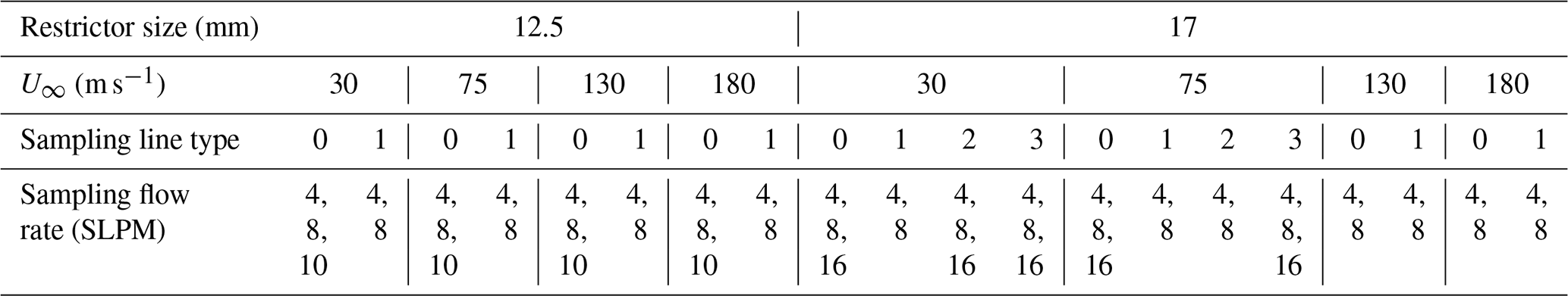
The sampling system of gas-phase H₂SO₄ measurements is shown in Fig. 1. The inlet is installed inside a wind tunnel test section that is 0.3 m × 0.3 m in dimensions (Fig. 1a). The wind tunnel is operated at different freestream velocities (30, 75, 130 and 180 m s⁻¹) that represent the range of aircraft speeds. This generates the different external and internal flows of the inlet. The flow from the sample tube was further sub-sampled to transfer H₂SO₄ through a sampling line to the CIMS instrument (Fig. 1b). The sampling tube shown in Fig. 1b is the actual sampling line used in-flight onboard the NSF/NCAR GV aircraft; it consists of a 33^′′ (0.84 m) long line, made of stainless steel, with several bending sections built to fit the requirements of installation on the aircraft. The CIMS instrument was located directly outside the wind tunnel testing section (Fig. 1c) and connected via the sampling line. The CIMS measured real-time chemical signal in response to the changes of wind tunnel conditions and sampling conditions. A mass flow controller (MFC) is used to throttle a pump to maintain and vary the sampling mass flow rate (see Table 1). In addition, to evaluate the role of shape of the sampling line on the gas-phase H₂SO₄ transmission efficiency, three other types of sampling lines are also tested. The schematic diagram of the tested lines is shown in Fig. 1d. The in-flight sampling tube with bends is labeled as type 1. The sampling tube labeled type 0 is a 33^′′ (∼ 0.84 m) straight tube of the same total length as the in-flight tube (i.e. type 1). The type 2 and type 3 tubes are the 40^′′ (∼ 1 m) straight tubes connected at the end of 33^′′ (∼ 0.84 m) straight tube with and without 90° bend at the end, respectively. We note that the wind tunnel setup has an extra 90° bend compared to actual in-flight sampling system. This extra bend is identical in all sampling lines and thus cancels out in relative comparisons of transmission between different line type configurations. Since the overall inlet transmission for the in-flight sampling system relies on piecing together the individual segments of the inlet assembly as shown in Fig. 5, the extra bend is not counted towards assessments of the aircraft configuration.

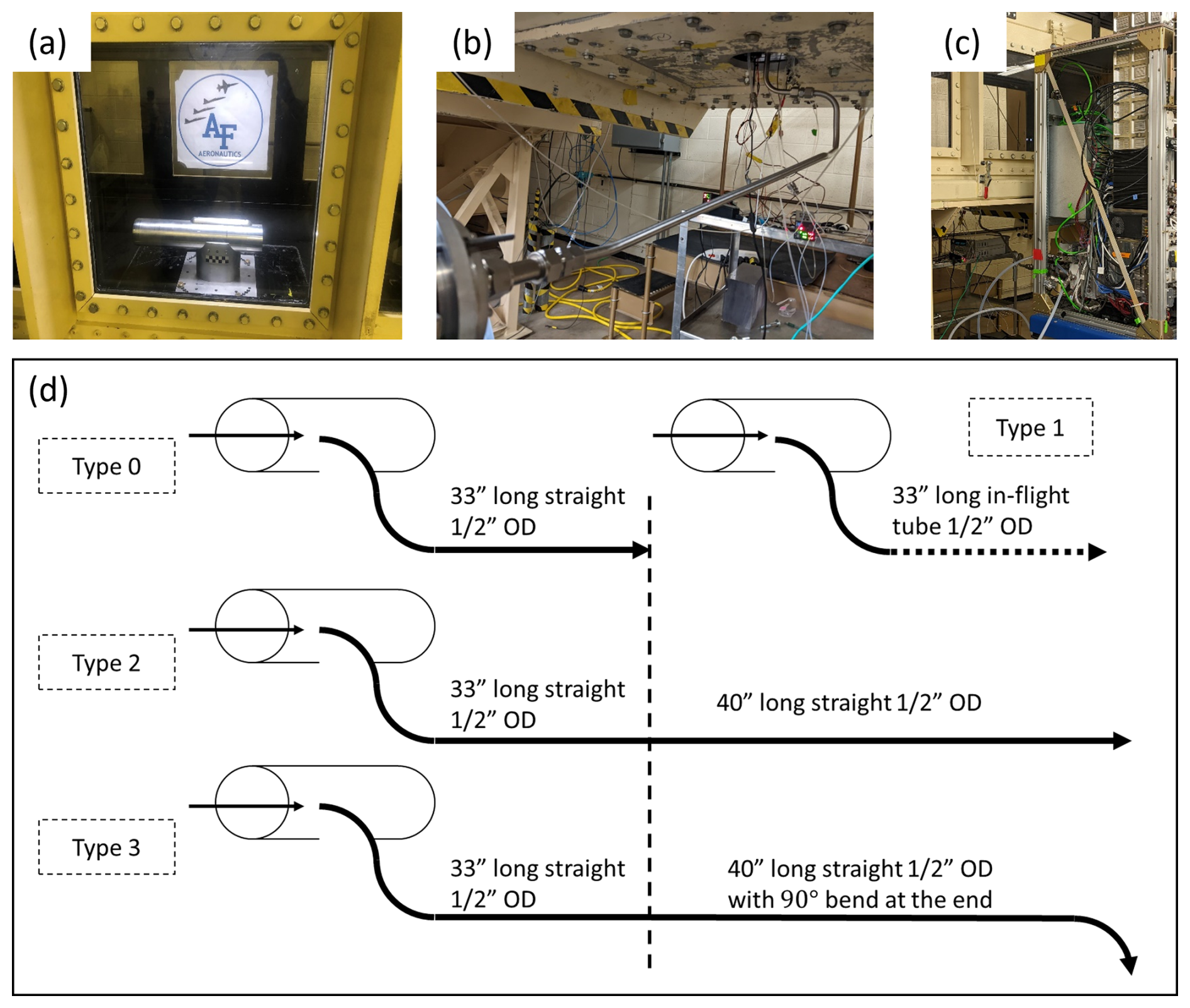
Figure 1 The wind tunnel experimental setup for H₂SO₄ transmission measurements. (a) Laminar gas inlet installed inside the wind tunnel test section. (b) The sampling lines used to connect the inlet with the CIMS instrument (c). The CIMS measured H₂SO₄ produced from the photolysis of H₂O at the tip of sampling tube inside the inlet under different line configurations, and wind tunnel conditions. (d) The schematic of four tested types of sampling lines; the line used in-flight is shown in panel (b) and referred to as type 1. The vertical dashed line marks the first section, which is the same length for each setup. For Type 1, the dashed line represents the different shape, but same length as Type 0.

2.2 Wind tunnel experiments

To conduct gas-phase H₂SO₄ measurement, additional supporting devices are integrated into the inlet (Fig. 2). As shown in Fig. 2, a UV source consisting of a Pen-Ray Mercury Lamp (90-0012-01), illuminates the inner shroud ∼ 10 mm in front of the sampling tube entrance. Ambient water vapor from the free stream is photolyzed as it travels into the inlet through the outer shroud. The photochemical dissociation (photodecomposition) of water vapor upon interaction with the UV light generates hydroxyl radicals.

$${\mathrm{H}}_{\mathrm{2}}\mathrm{O}+h\mathit{\nu }\to \mathrm{OH}+\mathrm{H}$$

The center of the inner shroud flow is sub-sampled by the sampling tube. SO₂ is injected (∼ 1 ppm tank mixture) via a port located near the entrance of the sampling tube. The hydroxyl radical interacts with SO₂, oxygen and H₂O to generate H₂SO₄ (Finlayson-Pitts and Pitts, 1999; Kolb et al., 1994). To prevent secondary radical cycling in the sampling tube, a small flow of Propane (∼ 100 ppmv) is added downstream. The sampled gas containing H₂SO₄ continues through the sampling tube until it reaches the entrance to the CIMS IMR. The nitrate CIMS used here has been described in detail in many previous publications (Eisele and Tanner, 1993; Mauldin et al., 1998), thus only a brief description will be given here. A schematic of the nitrate IMR is shown in Fig. 2c. The sample flow enters the IMR via the sample tube as shown. Inside the IMR, surrounding the sample tube is a flow of filtered air that has been “spiked” with a small amount of HNO₃. The outer annular region of this flow passes over an x-ray ionization source where the HNO₃ is ionized to form NO${}_{\mathrm{3}}^{-}$. Exiting the ionization region, the IMR flow consists of a central sample flow core, an annular region of unionized air surrounded by an outer region containing NO${}_{\mathrm{3}}^{-}$ ions. The NO${}_{\mathrm{3}}^{-}$ ions, but no the gas containing them, are then directed by means of electrostatic lenses into the central sample flow core where they interact with H₂SO₄ to form HSO${}_{\mathrm{4}}^{-}$ via:

$$\begin{array}{c}{\displaystyle }{\left({\mathrm{HNO}}_{\mathrm{3}}\right)}_n\cdot {\mathrm{NO}}_{\mathrm{3}}^{-}+{\mathrm{H}}_{\mathrm{2}}{\mathrm{SO}}_{\mathrm{4}}\to {\mathrm{HNO}}_{\mathrm{3}}+{\left({\mathrm{HNO}}_{\mathrm{3}}\right)}_n\cdot {\mathrm{HSO}}_{\mathrm{4}}^{-}\\ {\displaystyle }n=\mathrm{0},\mathrm{1},\mathrm{2}\end{array}$$

The ions are then directed by electrostatic lenses to the pinhole entrance of the Time of Flight mass spectrometer while the unionized gas is pumped away. The concentration of H₂SO₄ is then proportional to the ratio of the product ion signal, ${\left({\mathrm{HNO}}_{\mathrm{3}}\right)}_n\cdot {\mathrm{HSO}}_{\mathrm{4}}^{-}$, to the reagent ion signal, ${\left({\mathrm{HNO}}_{\mathrm{3}}\right)}_n\cdot {\mathrm{NO}}_{\mathrm{3}}^{-}$ (where n = 0, 1, 2). To account for processes that produce H₂SO₄ other than SO₂+OH, measurements were also made where propane, an OH scavenger, was added along with the SO₂. The product ion to reagent ion ratio from these measurements were subtracted from those without propane added to obtain the ratio due H₂SO₄ resulting from SO₂+OH only.

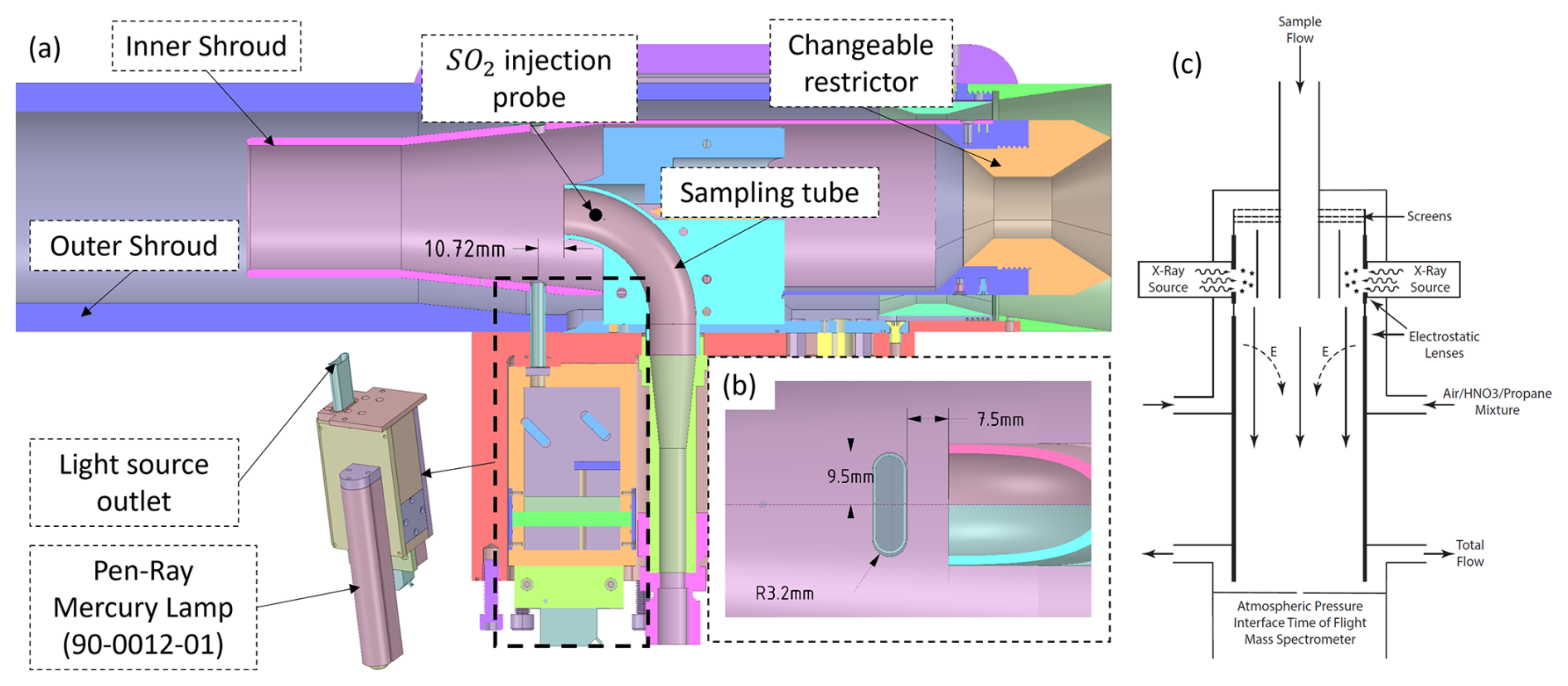
Figure 2 Cross-section view of the laminar gas inlet with UV lamp. (a) cross-section side view: shows different components of the inlet, incl. a 3D view of the UV source with mirror housing. (b) Cross-section top view: shows a detail view of the UV source outlet placement in front of the sampling tube entrance with dimensions. (c) CIMS Instrument Diagram.

In addition, to emulate the different operating conditions and to examine the impact from different system designs, four parameters were varied in the wind tunnel experiments, i.e., restrictor size of the aircraft inlet, free stream velocities (U_∞), sampling line type, and sampling flow rate. The testing cases are summarized in Table 1.

Table 1 Variables of the wind tunnel H₂SO₄ gas measurements.

2.3 Computational flow and mass transport modelling for sampling line

To inspect the correlations between internal flow features and gas measurement results, the CFD simulation results from previous inlet studies were used. The details of the aircraft inlet CFD modelling was described in our first laminar gas inlet paper (Yang et al., 2024). Compared to the freestream conditions considered in the first paper, since gas-phase H₂SO₄ measurements were also conducted at freestream velocity of 30 m s⁻¹; in gas measurement experiments, this freestream condition was added into our aircraft inlet simulations for both 12.5 and 17 mm restrictors. These additional simulations help facilitate direct comparisons with experimental results.

To predict and compare the gas transmission efficiency with measurements, we conduct flow and mass transport modeling in different sampling tube designs using the commercial code FLUENT 18.1 (ANSYS, NH), focusing on a 40^′′. (∼ 1 m) long straight tube with an ID of 10.7 mm. For the flow modelling, as most sampling flow rates (Table 1) result in a Reynolds number less than 2300 in the tube, the laminar flow model is used. In addition, considering the case when Reynolds number is close to 2300, a small disturbance in the tube can cause turbulent diffusion loss, we also used the transition SST k-ω model for flow modelling across both laminar and turbulent flow regimes (400 < Re < 7000+). Both flow models were used to examine the influence of diffusion coefficient in mass transport with and without any turbulence effect. Due to the symmetric nature of the tube, both a 2D-axisymmetric solver and a 3D solver were tested. The mesh is refined at the near wall region by applying bias mesh gradient for the 2D model and inflation method for the 3D model. The final mesh size was selected such that any further refinement resulted in a less than 1 % change in the flow velocity profile and mass fraction profile at the outlet of the tube. The final CFD model with a 3D geometry used ∼ 1.6 million cells to simulate flow under different boundary conditions.

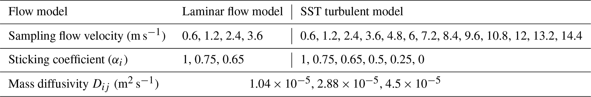
To model gas-phase mass transport, we consider the role of mass diffusion due to the concentration difference of gas-phase H₂SO₄ between the sample flow and the tube wall. In addition, we consider the diffusion process as binary diffusion, i.e., the model calculates gas-phase H₂SO₄ diffusion in the dry air. The binary diffusivity of H₂SO₄ in the laminar flow regime, referred as H₂SO₄ laminar diffusivity, is set as constant value of 1.04 × 10⁻⁵ m² s⁻¹. The Fick's law of diffusion is well applied for binary diffusion, and the model is applied in FLUENT 18.1. In addition, as the temperature gradient in the transmission line is insignificant, we neglect thermal diffusion loss. The simplified governing equation of our mass transport model expressed as:

$${\displaystyle \frac{\partial \mathit{\rho }{\mathit{w}}_i}{\partial t}}+\mathrm{\nabla }\cdot \left(\mathit{\rho }\mathit{v}{\mathit{w}}_{\mathit{i}}\right)=-\mathrm{\nabla }\cdot {\mathit{j}}_i,$$

where the mass fraction w_i represents the relative density of the diffusive species ρ_i (kg m⁻³) to the mixture density ρ (kg m⁻³), i.e. w_i = $\frac{{\mathit{\rho }}_i}{\mathit{\rho }}$. The v (m s⁻¹) represents the flow velocity. The expressions of mass flux j_i is determined by different flow models.

$$\begin{array}{c}{\displaystyle }{j}_i=-\mathit{\rho }{D}_{ij}\mathrm{\nabla }{\mathit{w}}_{\mathit{i}};\text{laminar flow model}\\ {\displaystyle }{j}_i=-\left(\mathit{\rho }{D}_{ij}+\mathit{\rho }{D}_{\mathrm{t}}\right)\mathrm{\nabla }{\mathit{w}}_{\mathit{i}},\text{turbulent flow model},\end{array}$$

where D_ij (m² s⁻¹) represents the laminar diffusivity, the subscript i represents the studied species (gas-phase H₂SO₄ or water vapor), the subscript j in our study represents dry air, and D_t (m² s⁻¹) represents the turbulent diffusivity.

For the laminar flow model, the laminar diffusivity D_ij is a constant value and only determined by the diffusing species, here gas-phase H₂SO₄. For the turbulent flow model, both laminar and turbulent diffusion contribute to the mass flux. The turbulent diffusivity D_t is calculated based on the turbulent viscosity predicted from the turbulent flow model, D_t = $\frac{{\mathit{\mu }}_{\mathrm{t}}}{{\text{SC}}_{\mathrm{t}}}$, where SC_t turbulent Schmidt number is dimensionless parameter that describe diffusion in mass transfer (Kang and Yang, 2014).

The different sampling conditions are modelled to investigate the factors that influence the gas transmission efficiency. The sampling flow rate and the mass fraction of H₂SO₄ on the wall are two key factors we investigated. The wall mass fraction boundary condition determines the probability that a gas molecule in the flow is captured on the wall. With a zero mass fraction boundary condition, the wall acts as a perfect sink and every gas molecule is accommodated on the wall. A wall mass fraction of one implies the wall maintains a layer of the gas on it, and the wall effectively does not accommodate any molecules from the flow. Boundary conditions between these two extreme values results in varying ability of the wall to accommodate gas molecules from the flow. Thus, the ratio of species mass fraction on the wall (w_wall) to that in the flow (w_flow) can be related to an equivalent wall sticking coefficient (α_i) for a selected gas species, calculated as:

$${\mathit{\alpha }}_i=\mathrm{1}-{\displaystyle \frac{w_{\mathrm{wall}}}{w_{\mathrm{flow}}}}={\displaystyle \frac{w_{\mathrm{flow}}-w_{\mathrm{wall}}}{w_{\mathrm{flow}}}},$$

where the mass fraction in the flow is the initial mass fraction of the studied species, and serves as the initial condition for the simulation. If the sticking coefficient was calculated using w_flow in one grid cell away from the wall, for an infinitely small grid cell the sticking coefficient would be equivalent to the mass accommodation coefficient at the wall.

In our simulations, we vary the wall mass fractions to vary the effective wall sticking coefficient. We vary the laminar or molecular diffusivities to represent different species or operating conditions. The entire set of boundary conditions for flow modeling are shown in Table 2. The operating conditions in the sampling line are obtained from aircraft inlet simulations under both ground level and high altitude conditions. All simulations were modelled assuming steady state flow.

Table 2 Boundary conditions for flow modelling in 40^′′ straight sampling line.

3 Results and discussions

The CIMS measurement data was systematically analysed with different experimental setups, operating conditions, and time periods. We calculate uncertainties using propagation analysis and the detailed error analysis is shown in the supplement. The CFD simulation results are used to compare and explain the observations from experimental results. The following sections will illustrate the data process and our findings.

3.1 Wind tunnel measurements

The transport efficiency measurements were made by analyzing the transport of species HSO${}_{\mathrm{4}}^{-}$ and HNO₃ ⋅ HSO${}_{\mathrm{4}}^{-}$ through the different sampling line types. These ion concentrations were recorded under different operating conditions by CIMS instrument (Fig. 1 and Table 1). Although applying the calibration factor of H₂SO₄ can covert these relative measurements to concentrations, the comparison between the sampling line types only relies on the use of relative information, and thus cancels out the calibration factor for sulfuric acid without adding uncertainty of calibration factor. As Fig. 3a is shown, the wind tunnel maintains the freestream velocity at different speeds for a measurement period and thus emulates different flight conditions for the gas-phase H₂SO₄ measurement. The temperature of the wind tunnel is increasing the longer the tunnel operates. Increases in temperature can provide slight variations in relative humidity, while the absolute humidity inside the wind tunnel is set by the outside air which re-circulates and cools the wind tunnel. The measurement of gas-phase sulfuric acid H₂SO₄ is presented as the sum of HSO${}_{\mathrm{4}}^{-}$ and HNO₃ ⋅ HSO${}_{\mathrm{4}}^{-}$ divided by the sum of nitrate parent ions (H₂SO₄ NCPS).

$${\displaystyle \frac{{\mathrm{H}}_{\mathrm{2}}{\mathrm{SO}}_{\mathrm{4}}}{{\sum }_{n=\mathrm{0}}^{\mathrm{2}}{\left({\mathrm{HNO}}_{\mathrm{3}}\right)}_n\cdot {\mathrm{NO}}_{\mathrm{3}}^{-}}}\cong {\displaystyle \frac{{\mathrm{HSO}}_{\mathrm{4}}^{-}+{\mathrm{HNO}}_{\mathrm{3}}\cdot {\mathrm{HSO}}_{\mathrm{4}}^{-}}{{\sum }_{n=\mathrm{0}}^{\mathrm{2}}{\left({\mathrm{HNO}}_{\mathrm{3}}\right)}_n\cdot {\mathrm{NO}}_{\mathrm{3}}^{-}}}$$

This ion ratio signal is unitless, and referred to as normalized counts (NCPS) or reagent normalized signal. A typical calibration factor for sulfuric acid is 5 × 10⁹ molec. cm⁻³ for the source configuration used (Eisele and Tanner, 1993; Mauldin et al., 1998); NCPS multiplied by the calibration factor yields a sulfuric acid concentration (1–2 × 10⁷ molec. cm⁻³) generated at the tip of the sampling tube in the aircraft inlet (Fig. 2a). In practice, the amount of sheath and total sampling flow were adjusted to give good NCPS signal, and the calibration factor is a function of the sample flow rate. However, the exact value of the calibration factor, and its uncertainty, does not affect the results, since our further analysis only relies on the ratio of NCPS values under comparable sample flow rates. The value of the calibration factor hence cancels out in relative statements about inlet transmission. For each measurement period, the CIMS instrument repeated three measurements of the raw data of H₂SO₄ NCPS with both background mode and signal mode (Fig. 3b). The background mode measures gas-phase H₂SO₄ background signal that is generated from dark sources, without addition of UV light. This mode provides the baseline of H₂SO₄ measurement under each operating condition. The signal mode provides the gas-phase H₂SO₄ measurement with additional hydroxyl radical, generated by photochemical decomposition of water vapor when sample air passes the UV light source. The signal depends on the operating conditions; i.e., NCPS of sulfuric acid decreases as the free stream velocity is increased.

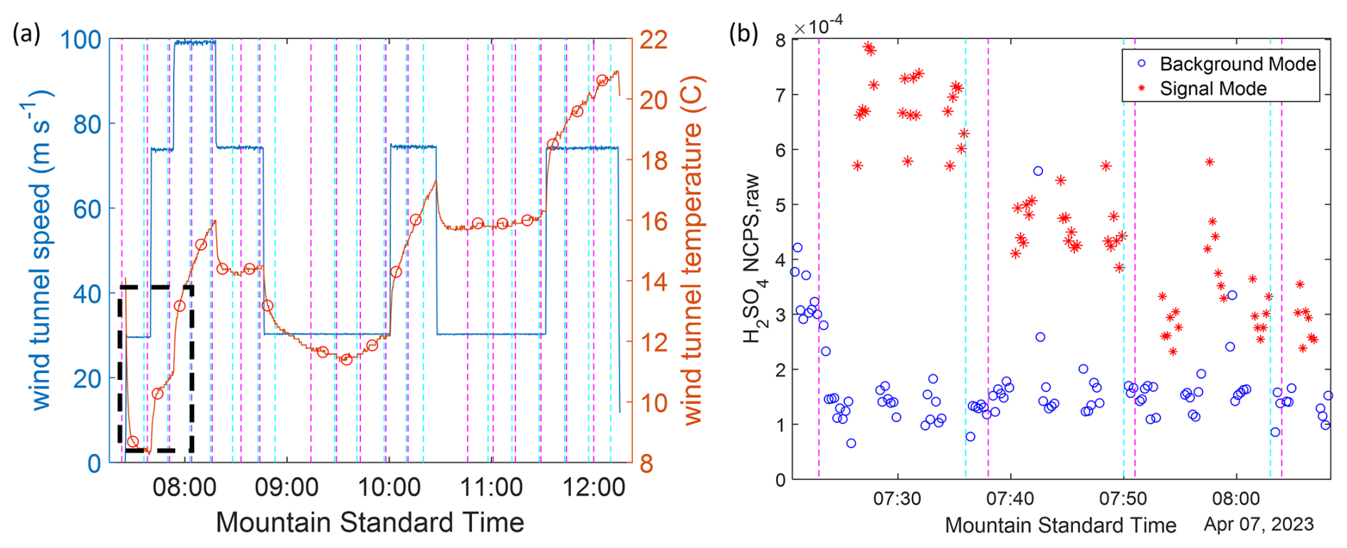
Figure 3 Wind tunnel conditions for experiments on 7 April 2023 (a) (blue line) free stream velocity inside the wind tunnel; (red line) temperature inside the wind tunnel, (black circles) averages for the gas measurement periods. (b) Real time H₂SO₄ NCPS raw measurements for the first three measurement periods marked in panel (a) (blue circles) background mode: detect hydroxyl radical pre-existing in the sample air; (red stars) signal mode: detect hydroxyl radical come from both sample air and water vapor photochemical decomposition. The magenta and cyan dashed lines for both figures mark the beginning and the end of each measurement case, respectively.

The difference between signal mode and background mode is proportional to the gas-phase H₂SO₄ concentration that is generated by the water vapor photolysis in the sample air (H₂SO₄ NCPS). Therefore, the measurement result is naturally dependent on the water vapor concentration in the ambient air. As the wind tunnel experiment was completed over multiple days, the repeated measurements under the same operating condition and setup shows significant differences that are the result of the changes in specific humidity under different weather conditions on different experiment days (Fig. S1 in the Supplement). These differences result in varying specific humidity inside the wind tunnel (Fig. S1a), and needed to be accounted for in comparing the measurement results of H₂SO₄ NCPS between different experiment days. A correction factor that normalizes changes in specific humidity (f_q) was defined as specific humidity (q) at each measurement period divided by the mean value of specific humidity among all measurements, and is found to largely reduce the differences among repeated measurements (Fig. S1b). The measurements of H₂SO₄ NCPS were normalized for constant specific humidity, H₂SO₄ NCPS/f_q, for further analysis and comparisons. The detailed analysis for raw data and correlation between flow and experimental results, H₂SO₄ NCPS/f_q, is shown in the Supplement.

3.2 Gas transmission efficiency comparisons

All types of sampling lines (Fig. 1d) and the different sampling flow rates are tested for gas-phase H₂SO₄ measurements using the 17 mm restrictor (Table 1). The normalized measurement results (H₂SO₄ NCPS/f_q) from 30 m s⁻¹ freestream velocity is shown in Fig. S5. The type 0 transmission line, due to the shortest length and minimum bends, shows the highest signal under comparable sampling flow rates, compared to other types of sampling lines. Increasing the length of the sampling line decreases the measured signal, consistent with additional losses in longer tubes. In addition, the 8 SLPM sampling flow rate maintains the highest quantity of signal, while 16 SLPM shows the lowest signal among three different sampling flow rates. This is specific to the instrument configuration used here, and related to the reaction time and flow characteristics inside the ion molecule reaction chamber of the CIMS instrument. Further analysis is outside the scope of this paper, which compares only ratios of normalized signal at comparable sampling flow rates. Similar trends are also observed in all cases of 75 m s⁻¹ freestream velocity. We are choosing the cases from the 30 m s⁻¹ freestream velocity for further analysis of the gas transmission efficiency in the sampling line due to the higher signal-to-noise. It should be noted that upstream effects (f_q and f_RT) are accounted for in the normalization of the signal, ensuring that the results for transmission are applicable to other free stream flow cases and restrictors of aircraft inlet as well. For comparisons with the same restrictor, f_RT cancels out.

The gas transmission efficiency is defined as the mass fraction (or concentration) of a molecule (here: H₂SO₄ or H₂O) at any cross-section along the sampling pathway compared to a reference mass fraction. Based on the wind tunnel experiments, we calculated the gas transmission efficiency of gas-phase H₂SO₄ measurement in the 40^′′ (1 m) tube as the ratio of normalized signal (H₂SO₄ NCPS/f_q) from the type 2 and type 3 sampling lines divided by the type 0, respectively, under each same sampling flow rate (f_RT cancels out). We use the mass fraction of the simulated H₂SO₄ at the outlet of the 40^′′ straight tube divided by its initial value at the tube inlet to calculate the gas sampling efficiency under different boundary conditions in the model. The experimental and simulated transmission are compared in Fig. 4. The experimental results clearly show the gas transmission efficiency in the 40^′′ tube is far below 1 for all sampling flow rates, which indicates a gas loss in this tube. In addition, the experimental results also show an increasing trend of the transmission efficiency as the sampling flow rate is increased. Moreover, the simulation results over predict the observed loss under the assumption that the mass fraction of H₂SO₄ is 0 on the wall, which corresponds to a sticking coefficient α_i = 1. Both the laminar flow model and the SST turbulent model have good agreement with the experimental results for sticking coefficients between 0.65 and 0.75 for gas-phase H₂SO₄. This agreement not only provides model verifications of the conclusion that reducing the residence time during the gas-phase species transport can reduce the gas transmission loss, but also compare well with the findings of the accommodation coefficient of H₂SO₄ is around 65 % to 75 % in other studies (Hanson, 2005; Pöschl et al., 1998). In Pöschl's paper, the mass accommodation for H₂SO₄ at 303 K under dry conditions (RH ≤ 3 %) has a best fit value of 0.65, with a physical upper limit of 1, and a lower statistical limit of 0.43. Hanson further discussed the impact of RH on the mass accommodation coefficient, and their data for H₂SO₄ show an average value of 0.76 for RH < 50 %. Our experimental results align reasonably closely with both previous laboratory studies, and the simulation results that apply a sticking coefficient for H₂SO₄ of 0.65 and 0.75 best describe the experimental observations in our aircraft inlet line. The sticking coefficient (α_i) we defined to set up the boundary conditions on the wall for our simulations is comparable to the mass accommodation coefficients measured at lower pressures in those previous studies. Therefore, we selected 0.7 as the average sticking coefficient and use ±5 % as uncertainty for further simulations. Moreover, the SST turbulent model overlaps with the laminar flow model when the flow rate is low and deviates when flow is outside the laminar flow regime. This observation provides further confidence in predicting the turbulent effects in our sampling system using the SST model, consistent with the findings comparing hotwire measurements of turbulence described in Part 1 of our inlet system analysis (Yang et al., 2024). Overall, the flow and mass transport models provide a reasonable description of the gas transmission loss in the entire inlet sampling system.

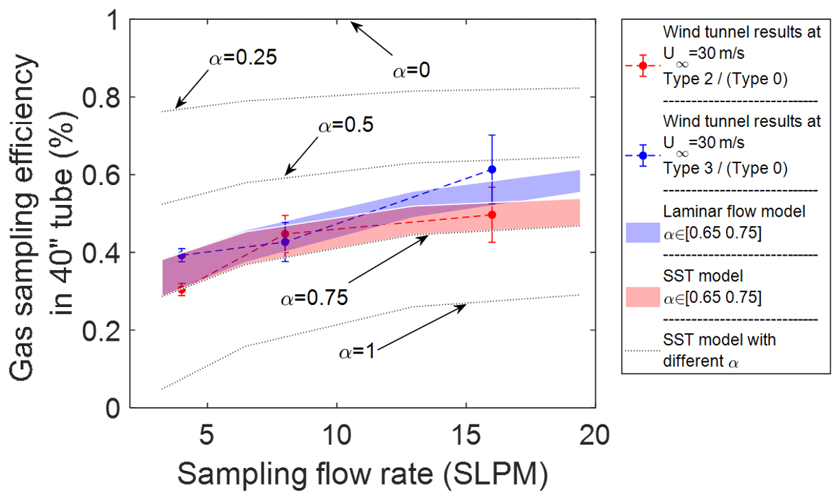
Figure 4 Comparison of different types of sampling tubes and the gas transmission efficiency: comparison of the gas sampling efficiency measured along 40^′′ (∼ 1 m) of a straight sampling tube with simulation results that vary the sticking coefficient, α_i. The error bar is uncertainty of the data which follows the description of propagation analysis in the Supplement.

3.3 Overall gas sampling efficiency of H₂SO₄

The verified CFD model assumed 70 % for the sticking coefficient α_i to set the boundary condition on the surface wall for gas-phase H₂SO₄ transport modelling. The gas-phase H₂SO₄ transmission efficiency of the overall inlet sampling system is calculated as a product of the transmission in different sampling sections. Specifically, Fig. 5 illustrates the individual components used to assess the overall gas-phase H₂SO₄ transmission efficiency: (a) transmission through the 12.5 mm restrictor inlet; (b) a straight 33^′′ (∼ 0.84 m) tube; (c) losses due to the shape factor (type 0 compared to type 1) due to the bending features (complements losses under b) with 10 % uncertainty; and (d) a straight 20^′′ (0.5 m) tube, respectively. The overall uncertainty in the transmission of the aircraft inlet sampling system combines the uncertainty in an ideal sampling system under various flow rates and flight conditions with a ±5 % variation of the selected sticking coefficient, and the shape factor (±10 %). In addition, to predict sampling efficiency for high altitude, we choose 4.5 × 10⁻⁵ m² s⁻¹ for the laminar diffusivity. This value is calculated based on the pressure and temperature at high altitude condition refer to the laminar diffusivity of gas-phase H₂SO₄ at ground level, D_ij = $D_{\mathrm{0}}{\left(\frac{T}{T_{\mathrm{0}}}\right)}^{\mathrm{1.75}}\frac{p_{\mathrm{0}}}{p}$, where the variables with 0 substitute present the reference value.

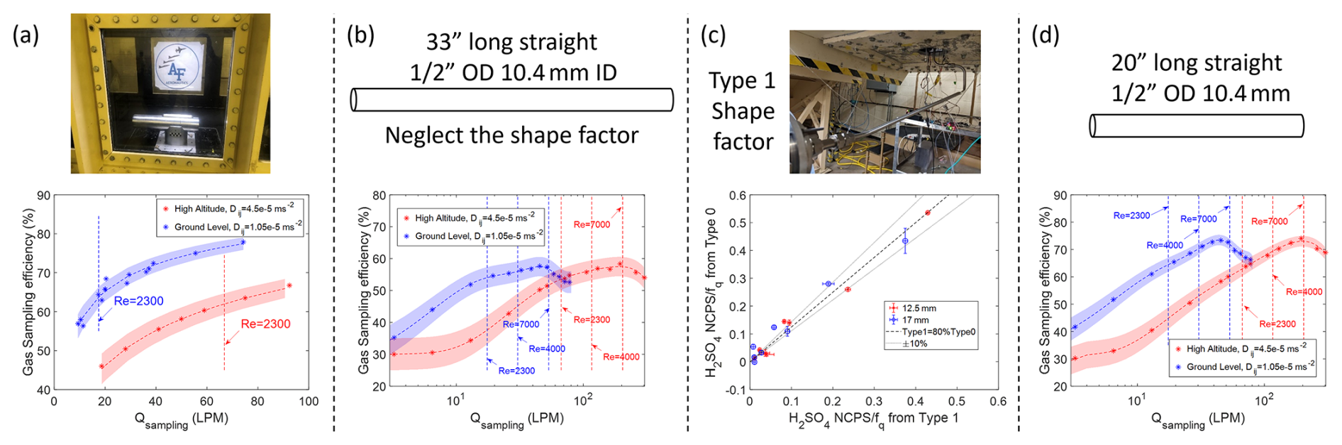
Figure 5 The gas-phase H₂SO₄ sampling efficiency in each partial section of the in-flight sampling system. The shaded areas in panels (a), (b) and (d) presents ±5 % uncertainty of the selected sticking coefficient (70 %); the overall sampling efficiency is shown in Fig. 6. (a) Inlet section: ambient air to the sampling outlet. (b) 33^′′ (0.84 m) straight tube. (c) Shape factor: compares type 1 and type 0 under same operating conditions; (dashed line) fitted as Type 1 = 80 % × Type 0; (dotted lines) ±10 % uncertainty of shape factor; (d) 20^′′ (0.5 m) straight tube to connect the CIMS in the aircraft configuration.

Notably, the individual sampling sections influence the gas-phase H₂SO₄ transmission efficiency differently. For the aircraft inlet section, the sample flow in the gas inlet is mainly impacted by the upstream turbulence. As a result, the gas sampling efficiency through this section shows a direct correlation with the sampling flow rate, and a difference at the two flight altitudes is mainly due to the laminar diffusivity at high altitude flight condition is set to be ∼ 5 times larger than ground level (Fig. 5a). Similarly, the sample flow in the sampling line is directly impacted by the characteristics of the local flow, the prediction of gas transmission efficiency inside the sampling line is also different between ground level and high altitude (Fig. 5b and d). At ground level, due to the higher flow density, the flow in the sampling tube is reaching the turbulent regime at a lower volume flow rate than at high altitude. In addition, the simulation results from both altitudes consistently show that the gas sampling efficiency can increase even when the sample flow enters the turbulent flow regime (Re > 4000). However, when flow reaches higher turbulent (Re > 7000), the sampling efficiency in sampling tube starts dropping again. This observation is due to the higher prediction of turbulent diffusivity, and indicates that the fate of the overall inlet gas transmission efficiency is determined by the local sampling flow rate (Q_sampling). For a selected sampling flow rate Q_sampling, increasing the inner diameter of the sampling tube (D) reduces the Reynolds number $\left(\mathit{Re}=\frac{\mathrm{4}Q\mathit{\rho }}{D\mathit{\pi }\mathit{\mu }}\right)$, and correspondingly the modeled turbulence in the sampling tube, with benefits for the overall gas transmission efficiency. In order to achieve the maximum gas transmission efficiency, our simulation results suggest that the optimized flow rate should maintain the Re in the sampling tube at ∼ 6000.

The overall gas sampling efficiency of the actual in-flight sampling system is calculated by multiplying the sampling efficiencies at the different sections and shape factors together. The results are shown in Fig. 6. We present the overall sampling efficiency of the actual in-flight sampling system at two altitudes as a function of the sampling flow rate. The shaded areas in Fig. 6 represent the largest range of uncertainty from ±5 % variation of sticking coefficient and ±10 % variation of shape factor. The simulation results indicate the overall gas sampling efficiency increases with sampling flow rate at both altitudes, and for most sampling conditions. This effect extends even when the sampling flow result in a Reynolds number past the laminar flow regime (Re ≤ 2300). These simulation results suggest that the residence time inside the inlet determines overall inlet transmission even well into the turbulent flow regime. However, the turbulent diffusivity predicted from the flow model increases as the Reynolds number increases. The overall sampling efficiency increases less rapidly, and eventually starts to decrease when the sampling flow rate reaches a much higher Reynolds number level (Re > 7000). The overall sampling efficiency is lower at high altitude compared to ground level if the results are compared at the same flow rate. This is because the laminar diffusivity at high altitude is 5 times more than the value set at ground level. Although the low altitude produces more turbulence and generates higher turbulent diffusivity, the significant change of laminar diffusivity also plays an important role in the sampling efficiency calculation. The simulation results suggest that the overall sampling efficiency of gas-phase H₂SO₄ for the actual in-flight sampling system can increase by a factor of 2 (from 12 % at 10 SLPM sampling flow rate to ∼ 20 % at ∼ 30 SLPM) by increasing the sampling flow rate at ground level. At high altitude, due to lower operating pressure resulting in a much higher laminar diffusivity, the overall sampling efficiency can increase to ∼ 20 % by increasing the sampling flow rate.

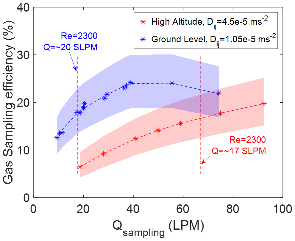
Figure 6 The correlation between overall gas transmission efficiency of H₂SO₄ and sampling flow rate Q_sampling (LPM) at ground level and high altitude. The dash lines mark the Reynolds Number in sampling line equal to 2300, which distinguish the laminar flow regime and beyond. The shade areas present the range of uncertainty from ±5 % variation of sticking coefficient and ±10 % variation of shape factor.

3.4 Extending transmission to other species

The transmission efficiency of H₂SO₄ can be extended also to other species or other operating conditions by directly changing the value of laminar diffusivity D_ij. However, a detailed treatment of other species requires a careful consideration of selecting the laminar diffusivity and sticking coefficients that is beyond the scope of this work. We therefore limit discussion on other species to sensitivity studies in a straight tube with varying laminar diffusivities (2.88 × 10⁻⁵ (m² s⁻¹) and 4.5 × 10⁻⁵ (m² s⁻¹)), and discuss some general considerations to inform future work. Simulations were performed for these laminar diffusivity values and varying the sticking coefficient from 0.1 to 1. The laminar or molecular diffusivity value of 2.88 × 10⁻⁵ (m² s⁻¹) is consistent with gas-phase water vapor at ground level. The value of 4.5 × 10⁻⁵ (m² s⁻¹) was selected for the gas-phase H₂SO₄ at high altitude flight condition. These values can vary depending on the species and operational conditions. In this study, we are not focusing on how to select laminar diffusivity values, but rather on showing the importance of choosing appropriate values.

The sample flow in the aircraft inlet section and the laminar diffusivity are mainly impacted by the upstream flow conditions. However, the laminar diffusivity affects gas loss in a relatively short distance compared to the sampling section. Thus, the gas sampling efficiency of the aircraft inlet section can be normalized for both altitudes and different diffusivities into a single fit function by using the volume flow rate divided by the laminar diffusivity, which is effectively the species Peclet number (Fig. S6). As such, the gas-transmission efficiency for aircraft inlet system can be parameterized and solved analytically for different sticking coefficient values for different species. However, no similar unified correlation of gas sampling efficiency can be found for varying diffusivities. This is because gas loss is a result of a complex combination of flow velocity, flow turbulence, and laminar diffusivity acting over long distance (∼ 1.3 m). In contrast, laminar diffusivity plays a secondary role in the aircraft inlet section, owing to the larger, dominating role of turbulence in this section of the aircraft inlet system.

We conducted a series of sensitivity studies to understand the transmission for species with different diffusivity through a straight tube. Figure 7 presents the results of gas sampling efficiency in a 33^′′ (0.84 m) straight tube between the maximum diffusivity of 4.5 × 10⁻⁵ (m² s⁻¹) and minimum diffusivity of 1.04 × 10⁻⁵ (m² s⁻¹) with different sticking coefficients at both ground level and high altitude for future interpolations. Comparing the results of transmission efficiency for the two species studied, it is observed that laminar (or molecular) diffusivity of a species plays a significant role in determining gas transmission efficiency for sticking ∼ 1. This dependence on laminar diffusivity, however, decreases for sticking coefficient values less than 0.25. This decrease in sensitivity of gas loss to laminar diffusivity with decreasing sticking coefficients makes the sticking coefficient qualitatively similar in principle to mass accommodation coefficient. The factor ∼ 4 range in laminar diffusivity (shaded area) also corresponds to the combined effect of temperature and pressure changes between the low and high altitude cases. For most tropospheric sampling, the effect from sticking coefficient will be minor for non-sticky molecules, but it gains in relative importance for sticky molecules sampled at low pressures; which was not the focus of the current study (windtunnel experiments at ground conditions), and deserves further attention in the future for high altitude sampling.

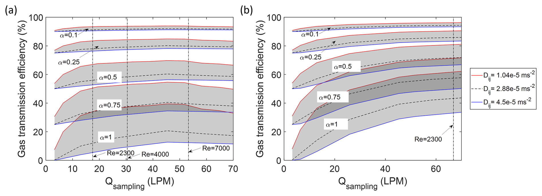
Figure 7 The comparisons of gas sampling efficiency between different laminar diffusivities at the sampling line section. (a) The correlation of gas sampling efficiency in 33^′′ (0.84 m) straight tube at ground level condition (1013 mbar). (b) The correlation of gas sampling efficiency in 33^′′ (0.84 m) straight tube at high altitude condition (220 mbar). The red line shows the sampling efficiency with diffusivity set as 1.04 × 10⁻⁵ m² s⁻¹. The blue line shows the sampling efficiency with diffusivity set as 4.5 × 10⁻⁵ m² s⁻¹. The shade areas covered the predicted sampling efficiency between these diffusivities at a selected sticking coefficient. The dark dash line in the shade areas shows the sampling efficiency with diffusivity set as 2.88 × 10⁻⁵ (m² s⁻¹).

This paper emphasizes the importance of choosing the correct diffusivity and sticking coefficient in predicting gas sampling efficiency of condensable vapors, in particular for highly diffusive condensable vapors (e.g., NH₃). Additionally, Khalizov et al. (2020) estimate that the limits of detection of oxidized mercury species are probably similar to those reported for H₂SO₄ (Eisele and Tanner, 1993; Mauldin et al., 1998; Zheng et al., 2010). Given the complexities of sampling oxidized mercury (Elgiar et al., 2024) significant transmission losses can be expected, with implications for the attainable detection limits in future attempts to sample oxidized mercury species using atmospheric pressure CIMS techniques (Khalizov et al., 2020). Moreover, the chemical properties of the inlet line can further influence transmission (e.g., pH, surface composition, reactivity). Determining these parameters and their transmission in flight warrants future work that is beyond the scope of this paper. The further warming of the sample in the tube as air transfers into the instrument aboard the aircraft depends on many parameters, including the temperature gradients along the tube as the flow enters the cabin air, the sampling flow rates, heat transfer from the tube to the gas, etc. These parameters and their influence on sampling efficiency are not well characterized and cannot be generalized; and it is not easily possible to model the full system accounting for all these parameters.

At high pressure, the wall loss rate is ideally expected to become independent of the reaction probability at the wall (i.e. the mass accommodation coefficient), and the wall loss is expected to approach the diffusion limit (Brown, 1978; Howard, 1979; Murphy and Fahey, 1987; Keyser, 1984). Here, however, we see that at ground-level, the sticking coefficient influences gas loss suggesting that the impact of the wall's sticking coefficient on wall loss does not exactly match that of the mass accommodation coefficient. It is possible that some of this dependance of gas loss on the sticking coefficient is a result of numerical errors in resolving flow features close to the wall, including the laminar sub-layer for turbulent flow.

4 Summary

In this paper, we describe an experimental approach to measure gas transmission efficiency of an aircraft inlet system using H₂SO₄ vapor and a high-speed wind tunnel setup. We use these observations to evaluate a CFD model of the aircraft inlet system; and use the validated CFD simulations to predict the overall sampling efficiency of gas-phase H₂SO₄ over a range of in-flight sampling conditions that span from the marine boundary layer (MBL) into the upper troposphere and lower stratosphere (UTLS). The inlet transmission for a condensable vapor like H₂SO₄ can be optimized using the sampling flow rate as a variable. For a realistic range of sampling flow rates, increasing the sampling flow rate can help cut transmission losses, and double the overall sampling efficiency of gas-phase H₂SO₄ compared to laminar flow conditions. The transmission of H₂SO₄ can reach up to 40 % in the UTLS, and up to 20 % in the MBL, owing primarily to the lower turbulent intensity and shorter residence time of air inside the sampling line under conditions typical of the UTLS.

Experiments and simulation results consistently support the conclusion that increasing the sampling flow rate can increase the gas transmission efficiency. These results challenge the widely accepted assumption that laminar core sampling, i.e., sampling from the core flow inside of an inlet line operated under laminar flow conditions, minimizes wall losses. This assumption is currently very widely used in laboratory and field experiments that sample ambient trace gases and aerosol species. Instead, shortening the residence time that air spends inside inlet lines is found to minimize wall losses well into the turbulent flow regime. The transmission increases initially due to a shorter residence time in the inlet, and then decreases as turbulent mixing increases and the laminar sub-layer thickness decreases in highly turbulent flow. The maximum inlet transmission is found for Re ∼ 6000, with lower transmission at both lower and higher Re numbers. For a condensable vapor like H₂SO₄, the effects to optimize transmission losses by optimizing the residence time can be as large as a factor of 2 over laminar core sampling.

To predict the transmission efficiency for other gas-phase species through this aircraft sampling system, the appropriate selection of the gas-phase diffusivity (D_ij) and sticking coefficient (α_i) of the species (i) is necessary. The overall sampling efficiency is calculated by combining the transmission efficiencies of the aircraft inlet and sampling line. For the aircraft inlet, a simulation-based function predicts transmission efficiency based on D_ij and α_i, as the gas loss is affected only by the upstream conditions regardless of altitude. Other factors can further affect transmission, i.e., pressure and temperature dependencies of the laminar diffusion coefficient, and for reactive species multiphase chemistry in addition to physical factors need to be considered. With the computational cost of modeling gas loss in the straight sampling line being reasonable, it is recommended to directly calculate the line's transmission efficiency using simulation models. Our flow analysis with straight tubes of variable lengths and sampling conditions, illustrates that the exact value of laminar (molecular) diffusion, D_ij, only plays a role for sticky gases with α_i > 0.25. By combining the transmission efficiencies from all sections and incorporating the sampling line's shape factor, the overall sampling efficiency of a gas-phase species for this aircraft-based sampling system can be estimated.