TROPOMI/WFMD v2.0: Improved retrievals of XCH₄ and XCO with XGBoost-based quality filtering

The TROPOspheric Monitoring Instrument (TROPOMI) on board the Sentinel-5 Precursor satellite provides daily global observations of atmospheric methane (CH₄) and carbon monoxide (CO) at relatively high spatial resolution. The dense spatial and temporal coverage is achieved by the instrument's wide swath, which permits detailed mapping of the worldwide distribution of these important atmospheric constituents. The adaptation and optimisation of the Weighting Function Modified Differential Optical Absorption Spectroscopy (WFMD) algorithm for the simultaneous retrieval of the column-averaged dry-air mole fractions XCH₄ and XCO from TROPOMI's shortwave infrared (SWIR) radiance measurements has proven to be a valuable complement and alternative to the operational TROPOMI products.

The latest release of the TROPOMI/WFMD product (version 2.0) includes several improvements expanding its suitability for a wider range of scientific applications. Data yield at mid and high latitudes has increased, accompanied by improved accuracy and precision according to the validation with the ground-based Total Carbon Column Observing Network (TCCON). These advancements are primarily due to more refined quality filtering that has been accomplished by replacing the previous Random Forest Classifier with the more efficient and potentially higher performing Extreme Gradient Boosting (XGBoost) algorithm in conjunction with improved training data incorporating an updated cloud product from the Visible Infrared Imaging Radiometer Suite (VIIRS) and the TROPOMI Aerosol Index. This enhanced training data set enables more reliable identification of cloudy scenes and mitigates issues related to specific aerosol events over bright surfaces. Importantly, as with previous product versions, the actual quality classification does not depend on the real-time availability of these external data products, which are only required during the training phase.

1 Introduction

Methane (CH₄) is the second most important anthropogenic greenhouse gas in terms of radiative forcing following carbon dioxide (CO₂). While it is less abundant in the atmosphere, the global warming potential of CH₄ by mass unit is significantly greater than that of CO₂ (Masson-Delmotte et al., 2021). However, thanks to its much shorter atmospheric lifetime of around a decade (Prather et al., 2012; Li et al., 2022), reducing CH₄ emissions will have a decisive impact on climate on a short timescale, so that rapid action can support measures to limit global warming to well below 2 °C above pre-industrial levels. Carbon monoxide (CO) is a reactive gas that is formed as a by-product during incomplete combustion and oxidation of hydrocarbons, including emissions from wildfires as a natural source. It contributes indirectly to climate change by depleting hydroxyl radicals (OH), which are critical for removing other gases that contribute to global warming, such as CH₄. At the same time, the oxidation of CO produces CO₂. Under certain conditions, CO also participates in photochemical reactions forming tropospheric ozone, which is itself a greenhouse gas. With a typical lifetime of 1 to 2 months, CO is a useful tracer for atmospheric air masses of anthropogenic origin. For sources that emit both CO and CO₂ simultaneously, it is feasible to use CO as a proxy for CO₂ emissions by using emission factors (Silva et al., 2013; Wu et al., 2022; Schneising et al., 2024). Because of these reasons, monitoring both gases helps to better understand atmospheric chemistry and guide efforts to mitigate climate change.

Satellite remote sensing has emerged as a useful method for tracking global distributions of CH₄ and CO. It thus offers unique insights into the underlying sources, sinks, and atmospheric transport processes. In particular, measuring upwelling shortwave infrared (SWIR) radiances is especially useful because of the sensitivity to changes in trace gas abundance throughout the entire atmospheric column. Instruments such as MOPITT (Terra) (Drummond et al., 2010), SCIAMACHY (ENVISAT) (Burrows et al., 1995; Bovensmann et al., 1999), and TANSO-FTS (GOSAT, GOSAT-2) (Kuze et al., 2016; Suto et al., 2021) have contributed important data on CH₄, CO, or both, depending on which spectral range each sensor covers.

Launched on 13 October 2017, TROPOMI on board ESA's Sentinel-5 Precursor satellite measures radiances across eight spectral bands from the ultraviolet (UV) to the SWIR (Veefkind et al., 2012) with daily global coverage and relatively high spatial resolution (5.5×7 km² at nadir in the SWIR bands, after August 2019). The unique capabilities of TROPOMI enable unprecedented mapping of CH₄ and CO distributions, supporting the detection of large-scale patterns as well as localised emission sources in a single satellite overpass. The data can be combined with targeted high-resolution airborne or satellite-based measurements with limited coverage (e.g., from GHGSat (Jervis et al., 2021)) in a tip and cue approach to zoom in on and quantify individual point sources detected by TROPOMI (Maasakkers et al., 2022; Schuit et al., 2023). In addition to the operational TROPOMI products for CH₄ (Hu et al., 2016; Hasekamp et al., 2022) and CO (Landgraf et al., 2016, 2022), the TROPOMI/WFMD product, which retrieves both gases simultaneously from a common spectral window (Schneising et al., 2019, 2023), has proven valuable as an independent data set in geophysical applications and in sensitivity studies to assess the robustness of findings with respect to the specific selection of the underlying data product (Veefkind et al., 2023; Nüß et al., 2025; Lindqvist et al., 2024).

A non-linear machine learning quality screening algorithm based on a Random Forest Classifier was implemented for the first time in the original TROPOMI/WFMD combined XCH₄ and XCO retrieval to exclude measurements that are insufficiently characterised by the tabulated forward model, which assumes rather simple physical conditions (e.g., cloud-free scenes) for fast processing (Schneising et al., 2019). Similar machine learning-based filtering techniques are now widely used in greenhouse gas retrievals from multiple satellite instruments (Keely et al., 2023; Borsdorff et al., 2024; Barr et al., 2025), reflecting a broader shift towards data-driven quality control in this field of remote sensing.

In this article, we present the recent updates that have been incorporated into the latest version of the TROPOMI/WFMD product (version 2.0). In particular, the Random Forest Classifier previously used for quality filtering has been replaced with the more efficient high-performance XGBoost algorithm, and the training data have been improved. The following sections provide a detailed account of these modifications, a comprehensive validation of the resulting data products, and demonstrate the consequential enhancements in data quality relative to the previous product version.

2 TROPOMI/WFMD algorithm improvements

The Weighting Function Modified DOAS (WFMD) algorithm retrieves column-averaged dry-air mole fractions of methane (XCH₄) and carbon monoxide (XCO) from SWIR radiances in the 2.3 µm spectral range measured by TROPOMI and is described in detail in Schneising et al. (2019, 2023). Therefore, only the main aspects are briefly summarised here. WFMD uses a least-squares approach to scale pre-defined vertical profiles and fits a linearised radiative transfer model based on SCIATRAN (Rozanov et al., 2002, 2014) to the logarithm of the sun-normalised radiance. A look-up table enables efficient retrievals of the vertical columns of the targeted species by covering various atmospheric conditions. The retrieved columns are converted to XCH₄ and XCO using dry air columns from the European Centre for Medium-Range Weather Forecasts (ECMWF) adjusted for the higher resolved actual surface elevation of the individual satellite scenes. A machine learning-based classifier filters low-quality scenes using cloud data from the Visible Infrared Imaging Radiometer Suite (VIIRS) onboard Suomi NPP (Hutchison and Cracknell, 2005) in the training phase. To mitigate residual albedo-related biases in XCH₄, a random forest regressor with shallow decision trees (leaf nodes ≪ training scenes ≪ all scenes) is trained on a small spatio-temporally constrained subset using a small number of features and the SLIMCH4 climatology (Noël et al., 2022) as a low-resolution reference. This post-processing correction method is statistically robust and generalises effectively to unseen data (Schneising et al., 2023). No similar correction is required for XCO due to its larger natural variability and relaxed quality requirements.

2.1 General processing improvements

TROPOMI/WFMD v2.0 introduces several improvements aimed at enabling more robust results in scientific applications. It consistently uses TROPOMI Level 1b V02.01.XX files as input, ensuring the inclusion of the latest instrument calibration. The first part of the split spectral fitting window described in Schneising et al. (2019) contains a continuum-like region (with virtually no absorption by atmospheric constituents), which serves to determine the apparent albedo in the preprocessing step in order to disentangle surface reflection and molecular abundances in the actual fitting procedure. In v2.0, the first part of the retrieval window has been slightly extended by 0.4 nm at the long-wavelength end and now covers the spectral range from 2311–2315.9 nm, while the enclosed near-continuum itself remains unchanged. The extension aims at improving the transition to the region with stronger molecular absorption features captured in the second part of the fitting window (2320–2338 nm) and may enhance the signal-to-noise ratio and baseline fitting, thereby supporting more stable and precise retrievals. The position of the fitting window and the continuum-like interval it contains is shown together with the corresponding molecular absorption features in Appendix A in an example spectral fit.

Another update in v2.0 is the usage of a hybrid sigma-pressure vertical coordinate system consisting of 31 layers to provide the prior profiles and averaging kernels, replacing the previous pure sigma coordinate system with 20 layers, in which each layer represented an equal fraction of the total surface pressure. Figure 1 compares the two vertical discretisations using an example of surface elevation variation. The new hybrid layering combines terrain-following characteristics near the surface with enhanced vertical resolution in the lower atmosphere and fixed reference levels in the upper atmosphere. The increased near-surface vertical detail in the prior and averaging kernel information supports the consideration of surface pressure mismatches during comparison with other measurements (e.g., for validation) or during assimilation in inverse modelling frameworks. Such mismatches can occur due to local horizontal displacement relative to comparison measurements or from the coarse horizontal resolution of models. The enhanced vertical representation may therefore facilitate better harmonisation of these inherent differences, especially over complex terrain.

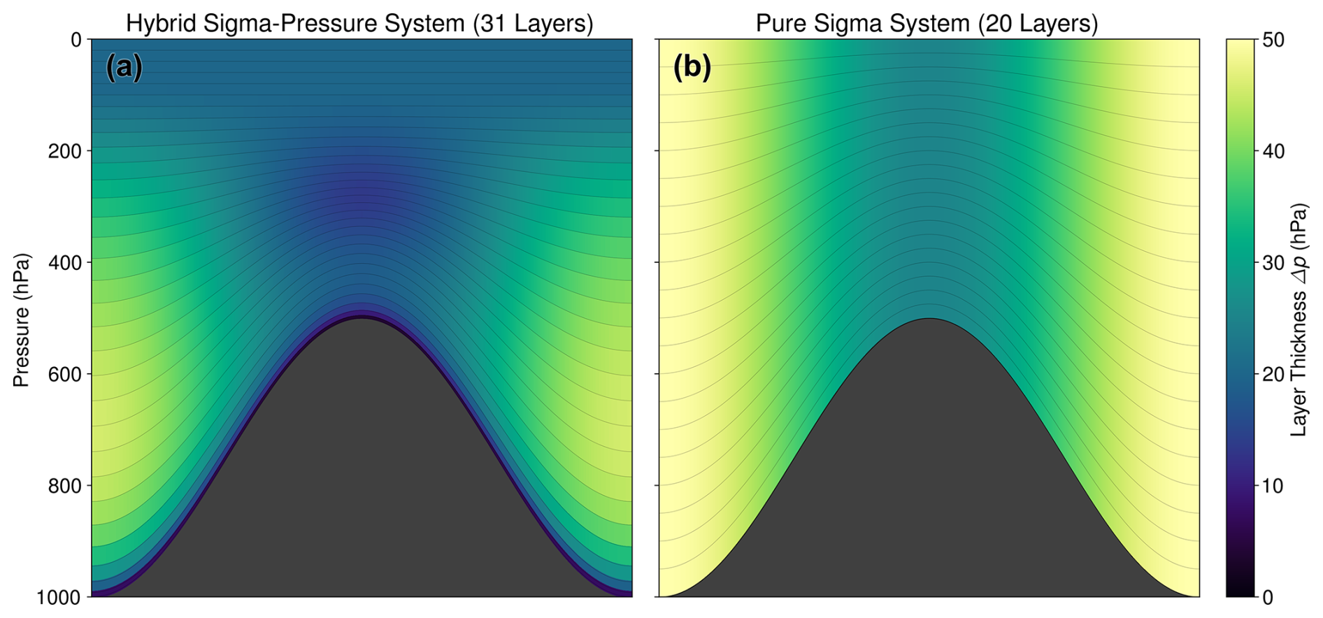
Figure 1 Comparison of (a) the 31-layer hybrid sigma-pressure vertical coordinate system used in TROPOMI/WFMD v2.0 with (b) the previous 20-layer pure sigma coordinate system. The dark grey area illustrates exemplary surface elevation variation in x-direction. The associated pressure layer thicknesses are colour-coded. The perceptual uniform colormap used here and in many other figures is described in Appendix B.

2.2 XGBoost-based quality filtering

In earlier versions of the product, quality filtering was accomplished using a Random Forest classifier (Schneising et al., 2019, 2023), since it delivers robust results that are largely insensitive to fine-tuning of the hyperparameters (Tantithamthavorn et al., 2019). Random Forest is a bagging-based ensemble learning method that trains the involved decision trees in parallel. In the standard implementation, these trees are deep and unpruned. All trees train independently on bootstrapped subsets of the training data, with a random subset of features made available at each split (Breiman, 2001). This double randomisation of the training process implies that each tree is created from a different subset of data and features, which decorrelates the individual trees from each other and reduces overfitting by means of the imposed diversity within the ensemble. The final predictions are made by majority voting among the trees, which reduces variance, as the collective decision-making process aggregates the results of the heterogeneous ensemble members. For a global quality filtering task that spans a wide range of surface types, atmospheric states, and illumination conditions, achieving sufficient ensemble diversity quickly drives up model size and memory demands, which limits extensibility to additional effects. In particular, infrequent but physically consistent quality-degrading conditions, such as specific aerosol events over bright surfaces targeted in the updated product version, may not be optimally captured by a Random Forest classifier, as its ensemble-averaging strategy risks diluting such sporadic signals.

To address this limitation, the latest product TROPOMI/WFMD v2.0 uses Extreme Gradient Boosting (XGBoost) (Chen and Guestrin, 2016), providing a more compact and computationally efficient framework for comprehensive quality filtering. XGBoost builds trees sequentially, with each new tree aiming to correct the residual errors of the preceding ensemble. To achieve this, the respective new tree is trained to predict the negative gradient of the current loss function in order to determine the direction and magnitude of the required correction. By iteratively adding these correction trees, XGBoost reduces bias and variance, often surpassing the predictive performance of bagging-based models. The one-time training process is slower due to its sequential nature, but the resulting model tends to be shallower and more optimised, which is beneficial when used in resource-constrained environments. Unlike Random Forest, which usually performs well with default settings, XGBoost is more sensitive to hyperparameter optimisation due to the complex way its tuning parameters interact with each other. For the TROPOMI/WFMD v2.0 quality filter, the Python package xgboost is used, and tuning efforts focussed on balancing model simplicity with generalisation ability, resulting in the following parameter values, which demonstrate the importance of carefully tuning XGBoost to create a maximally robust and generalisable model.

2.2.1 Model training and internal evaluation

To prevent overfitting, a conservative 𝚕𝚎𝚊𝚛𝚗𝚒𝚗𝚐_𝚛𝚊𝚝𝚎=0.03 was chosen to shrink the weights for the corrections by new trees, with the trade-off that more boosting rounds are required to compensate for the slower (but more accurate) learning. The complexity of the individual trees was constrained with 𝚖𝚊𝚡_𝚍𝚎𝚙𝚝𝚑=8 and 𝚖𝚒𝚗_𝚌𝚑𝚒𝚕𝚍_𝚠𝚎𝚒𝚐𝚑𝚝=4 in order to obtain suitable pruning without uncontrolled growth. An increase in the generalisation capability to unseen data was achieved by adding a random component to the training process via 𝚜𝚞𝚋𝚜𝚊𝚖𝚙𝚕𝚎=0.7 and 𝚌𝚘𝚕𝚜𝚊𝚖𝚙𝚕𝚎_𝚋𝚢𝚝𝚛𝚎𝚎=0.7. This means that each tree of the model is trained on randomly selected 70 % of the training data using 70 % of the available features, which makes the model less likely to fit to noise or irrelevant patterns in the training data. Besides the tree construction and sampling parameters, there are also other regularisation parameters in addition to the already discussed learning rate: 𝚐𝚊𝚖𝚖𝚊=0.2 requires that nodes in a single tree are only added if the associated loss reduction is large enough, thus impeding unnecessary splits; 𝚕𝚊𝚖𝚋𝚍𝚊=1 controls the L2 regularisation of the leaf weights by encouraging the model to find a simpler solution that generalises better to unseen data. While 𝚕𝚊𝚖𝚋𝚍𝚊 is applied during tree creation, 𝚕𝚎𝚊𝚛𝚗𝚒𝚗𝚐_𝚛𝚊𝚝𝚎 scales down the final tree weights at the moment it is added to the ensemble.

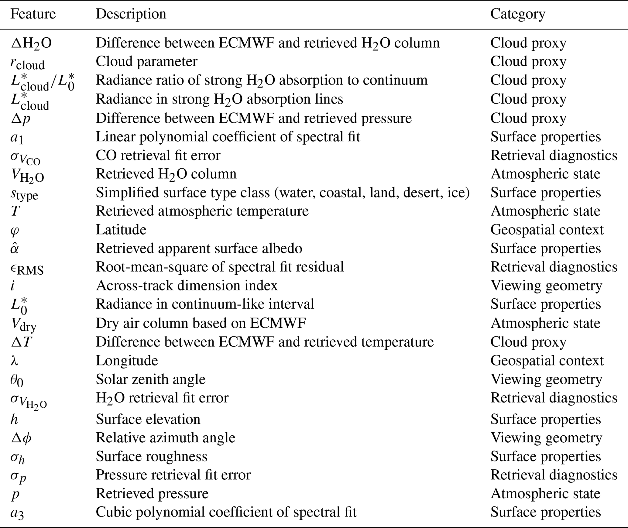
The XGBoost classifier was trained using data from 38 randomly selected days distributed across 2020 and 2021, with the additional requirement that all seasons are adequately represented. This sampling strategy covers all physically observable combinations of latitude and solar zenith angle and captures a broad range of atmospheric conditions, while keeping the overall data set size manageable. The training truth for the quality filter was informed by an updated cloud product from the Visible Infrared Imaging Radiometer Suite (VIIRS; S5P S-NPP Cloud processor version V01.03.00 based on the VIIRS Enterprise Cloud Mask) and the TROPOMI Aerosol Index (V02.04.00), aiming at improved identification of cloudy scenes and mitigation of issues arising from specific aerosol events over bright surfaces. The classification task involves a clear class imbalance, with good quality observations (class 0) representing a minority (p=0.151). The set of 26 features used in XGBoost (listed in Sect. 2.2.2) remains identical to the quality filter of v1.8 (Schneising et al., 2023) and comprises only intrinsic parameters available from preceding processing. This means that the quality filter remains independent of real-time availability of external cloud and aerosol information during the actual quality prediction.

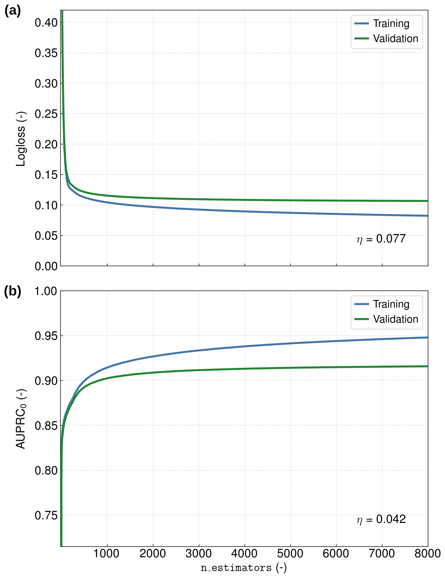
Figure 2 Training and validation performance, measured by (a) Logloss and (b) the Area Under the Precision-Recall Curve (AUPRC, see main text for details) for class 0 (good quality), as a function of boosting rounds, illustrating stable convergence without notable overfitting. The relative gap metric η quantifies how large the final training-validation gap is relative to the achieved gain on the validation set over the baseline. A small value of η indicates that the fitted model generalises effectively to unseen data.

Model performance was assessed using completely independent data from 2022, a year that was not involved at all in the training process. To monitor and prevent overfitting, early stopping was applied during training (𝚎𝚊𝚛𝚕𝚢_𝚜𝚝𝚘𝚙𝚙𝚒𝚗𝚐_𝚛𝚘𝚞𝚗𝚍𝚜=25) using the Logloss metric for progress tracking. Logloss was chosen because it corresponds directly to the objective function that is minimised in XGBoost training, thus ensuring consistency of the evaluation step with the underlying optimisation process. As a performance measure, Logloss evaluates the calibration quality of predicted probabilities across all classes. Early stopping intervened after 8000 boosting rounds (𝚗_𝚎𝚜𝚝𝚒𝚖𝚊𝚝𝚘𝚛𝚜) because the Logloss on the validation set had not improved in 25 consecutive rounds, revealing that the learning progress had already levelled off significantly. According to Fig. 2, the corresponding validation Logloss curve decreases monotonically during the 8000 boosting rounds to values substantially below the baseline entropy of $-\left(p\log \right(p)+(\mathrm{1}-p\left)\log \right(\mathrm{1}-p\left)\right)\approx \mathrm{0.424}$ expected under the prevalence p of class 0.

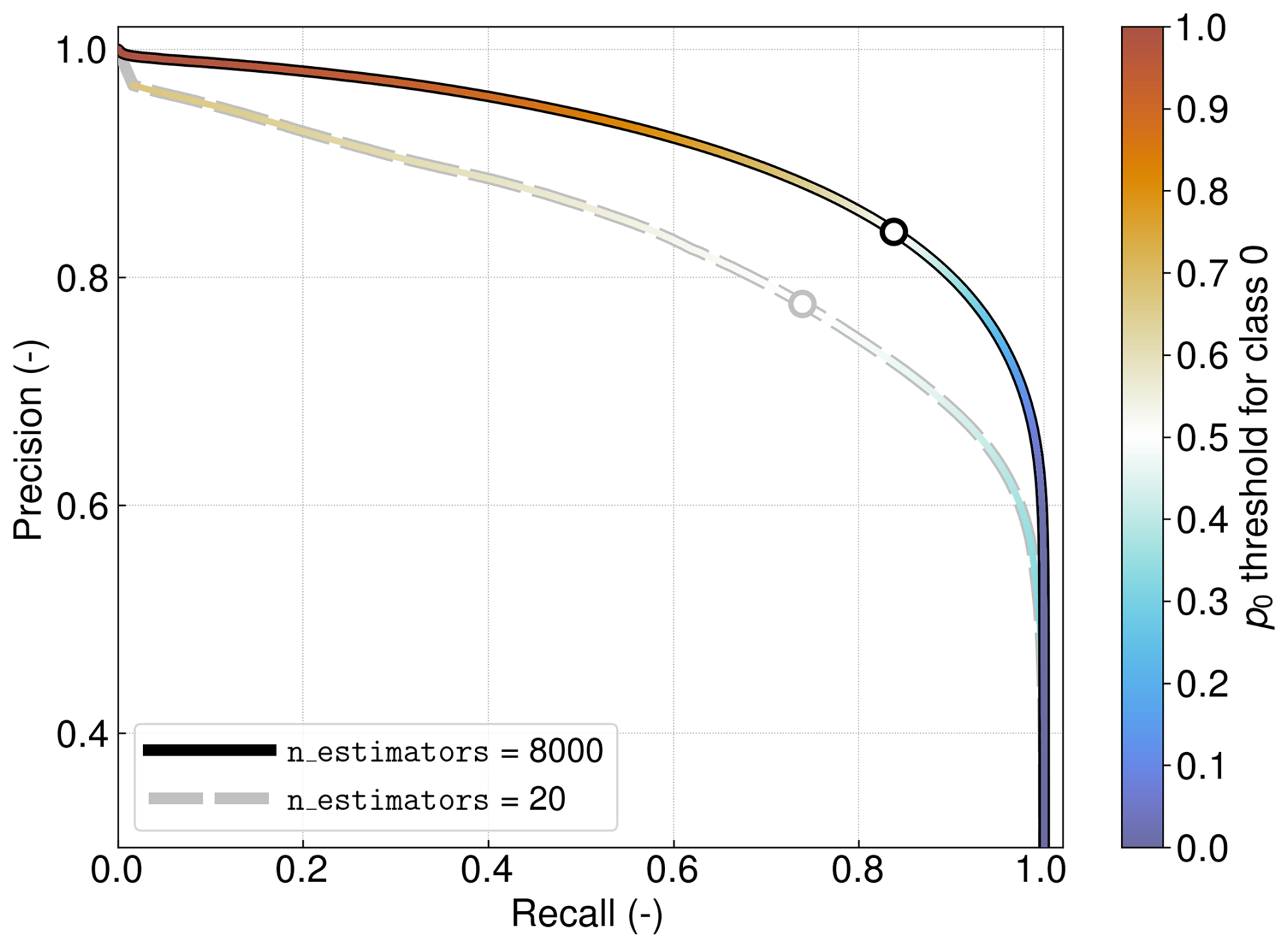
Figure 3 Final precision-recall curve of the XGBoost classifier for class 0 (good quality) evaluated on the validation set compared to a respective curve for an early boosting round. The curves are colour-coded according to the corresponding decision threshold p₀, illustrating how model performance changes as the threshold varies. The circles represent the standard threshold p₀=0.5 used for assigning the class label 0 in the TROPOMI/WFMD v2.0 quality filter.

To interpret the magnitude of potential overfitting, we quantify the achieved gain on the validation set as the decrease in Logloss relative to the baseline entropy and define the relative gap metric η to be the ratio of the final training-validation gap to this gain. This metric offers an intuitive way to assess overfitting and how well a model generalises to unknown data that was not used in training. In the present case, η is only about 8 %, demonstrating that the final training-validation gap is negligible relative to the validation improvement and that the vast majority of the model's fitted relationships generalise effectively, with overfitting being negligible when assessed in terms of Logloss.

In addition to the previous assessment, potential overfitting was further evaluated using the Area Under the Precision-Recall Curve (AUPRC), which is particularly suitable for the present application due to the considerable class imbalance. The AUPRC is specifically meaningful under these conditions as it captures the trade-off between recall (coverage of actual positives) and precision (correctness of positive predictions). It penalises false positives more than other metrics such as the Area Under the Receiver Operating Characteristic Curve (AUROC). This emphasis is in line with practical considerations in quality filtering, where false positives (e.g., cloudy scenes that incorrectly pass the quality filter) can introduce systematic retrieval biases, as such scenes are typically not well characterised by the tabulated forward model.

Since a random classifier would produce an AUPRC close to the prevalence p, any substantial improvement over this baseline clearly signals successful distinction between classes. Analogous to the Logloss evaluation, the relative gap metric η is defined as the ratio of the final training-validation gap to the gain achieved and quantifies potential overfitting in terms of AUPRC. As shown in Fig. 2, the AUPRC curve of the validation data set rises monotonically to high values close to the theoretical maximum of 1.0 and reaches approximately 0.92 after the completed 8000 boosting rounds, which is about six times the prevalence baseline. The corresponding η is a mere 4 %, showing that the final difference between the training and validation curves is negligible compared to the improvement achieved on the validation set, which is consistent with the conclusions from the Logloss analysis. Overall, the consistent performance across the complementary evaluation metrics Logloss and AUPRC shows that the implemented XGBoost model validly distinguishes between classes under imbalanced conditions, without showing appreciable signs of overfitting.

The resulting precision-recall curve is shown in Fig. 3 with colour-coded decision threshold p₀, which is the minimum level of prediction probability for assigning an instance to class 0 (good quality). The graph illustrates the classifier performance trend when varying the threshold, supporting a more reasonable choice of p₀ based on the required balance between precision and recall. In the context of a quality filter, it is helpful to recognise that recall and data yield are positively correlated. Increasing the threshold results in higher precision (reducing the number of false positives) but at the expense of lower recall, meaning that more true positives are missed. Conversely, a lower threshold raises recall, but it also leads to more false positives. For the TROPOMI/WFMD v2.0 quality filter, the standard threshold p₀=0.5 is used to assign class labels because it is a transparent default that is easy to interpret. This value reflects the point at which the model is equally confident in assigning either class, which is commonly chosen when there is no strong preference for favouring precision over recall. In the current product, this threshold is fixed by design and only the resulting binary quality flag is provided, prioritising simplicity and consistent data quality over enabling user-controlled adjustment of the decision threshold.

2.2.2 Feature importance

The XGBoost quality filter is trained on a set of 26 input features, identical to those used in the Random Forest classifier of v1.8 (Schneising et al., 2023). For transparency and reproducibility, all variables are listed in Table 1. The features are divided into the following groups according to their functional role: cloud proxies, surface properties, viewing geometry, atmospheric state, retrieval diagnostics, and geospatial context. This categorisation enables a process-oriented interpretation of model behaviour extending beyond the influence of individual variables.

Table 1 Input features used by the quality filter, ordered by decreasing mean absolute SHAP importance.

Several of these features provide clear indications of cloud cover. A prime example is the cloud parameter r_cloud, which relates the measured radiances in strong H₂O absorption bands to reference radiances for cloud-free conditions (Heymann et al., 2012). The feature set also includes related radiance-based indicators, which respond in a similar way when clouds are present. Another, conceptually different approach compares ECMWF reanalysis fields with the corresponding retrieved state variables, on the assumption that systematic deviations may occur when clouds interfere with the measurements. High positive values of ΔH₂O and Δp, for example, are a typical signature of optically thick clouds that mask part of the atmospheric column. The sign of ΔT, on the other hand, is less consistent in cloudy conditions and does not provide an equally clear diagnostic.

The interpretability of the model and the importance of the included features are assessed using SHAP (SHapley Additive exPlanations) (Lundberg and Lee, 2017; Lundberg et al., 2020). SHAP values decompose individual predictions into additive contributions from each input feature, allowing both global ranking of feature importance and local interpretation of specific decisions. Figure 4 summarises the SHAP analysis for the validation data set. Features are ordered by their mean absolute SHAP values, while violin plots illustrate the full distribution and direction of their contributions. Positive SHAP values shift predictions towards the “bad” quality class. The five most influential features are all cloud proxies. In line with physical expectations, high values of these variables correspond to positive SHAP contributions and therefore to rejection by the quality filter. This behaviour reflects either direct shielding of the atmospheric water vapour column by clouds or enhanced radiance in strong H₂O absorption bands, which would remain low under clear-sky conditions due to near-saturation of the relevant spectral lines.

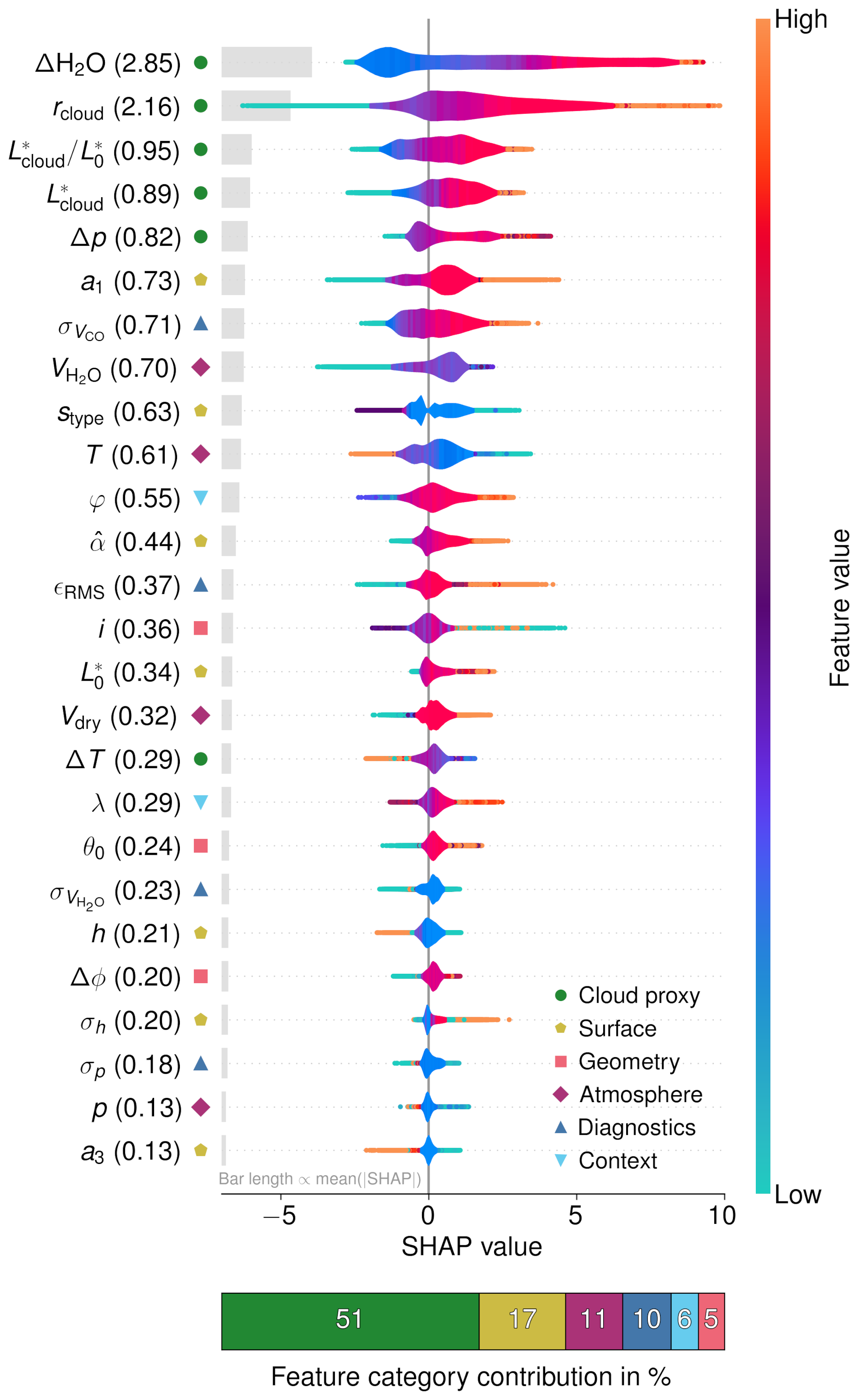
Figure 4 SHAP-based feature analysis for the XGBoost classifier evaluated on the validation data set. Mean absolute SHAP values (shown in brackets next to each feature) and the corresponding grey bars summarise global feature importance. Violin plots illustrate the distribution and sign of feature contributions, coloured by feature value. The stacked bar shows the relative contribution of the different feature categories to the total mean absolute SHAP.

Totalling the SHAP scores by feature category offers a nuanced view of the broader factors that shape the classifier's decisions. Cloud proxies have the greatest impact, accounting for 51 % of the total mean absolute SHAP value. Next come surface properties at 17 %, followed by atmospheric state variables (11 %), retrieval diagnostics (10 %), geographical context (6 %), and viewing geometry (5 %). The weighting of these factors reveals a defined hierarchy in the classification process: the model is primarily based on physically motivated cloud indicators, while the other feature groups provide contextual assistance that refines the interpretation. The relatively modest influence of geographical context demonstrates that latitude and longitude serve as secondary decision modifiers rather than directly driving climatological filtering.

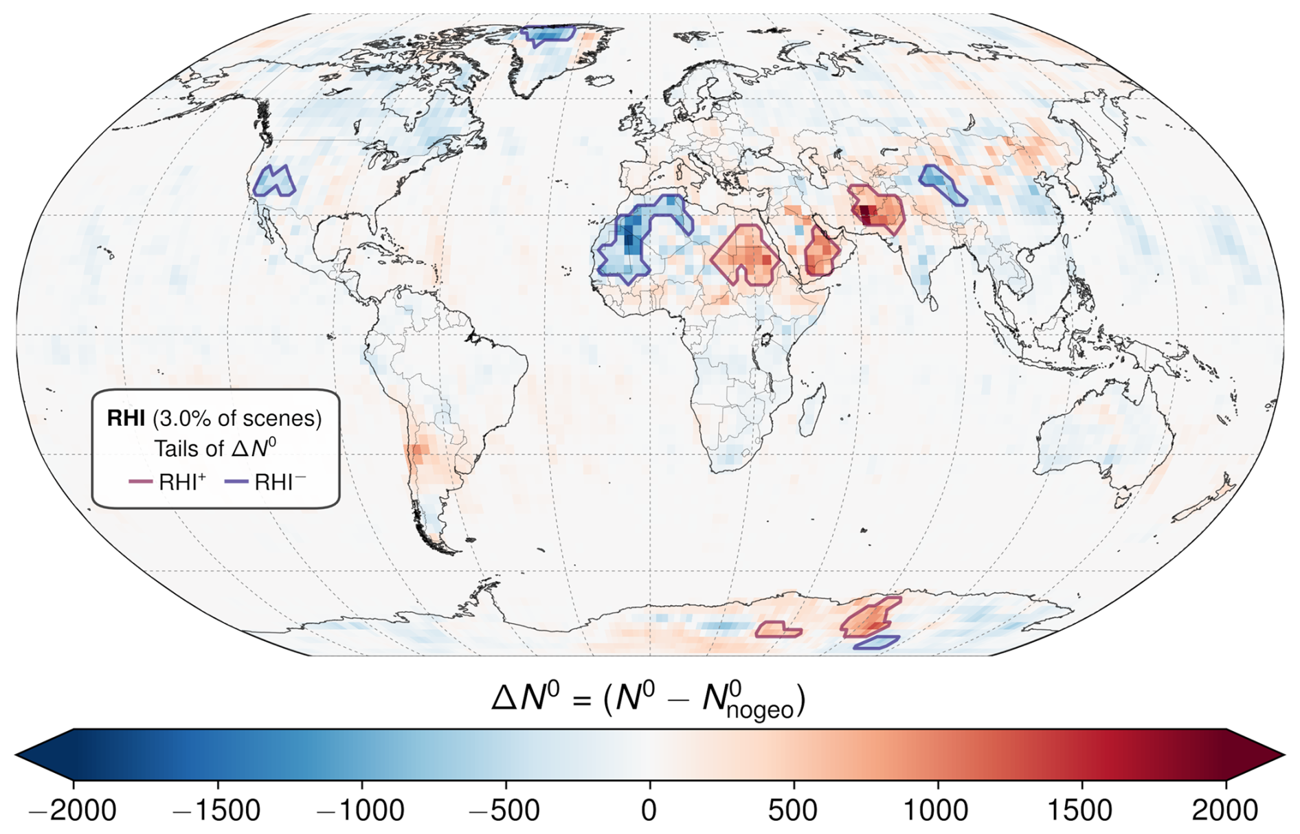
Figure 5 Spatial distribution of changes in the number of scenes passing the quality filter ΔN⁰, resulting from the inclusion of latitude and longitude as input features. The analysis is based on the validation data set and evaluated on a ${\mathrm{2.5}}^{\circ }\times {\mathrm{2.5}}^{\circ }$ grid. Spatially connected clusters of grid cells in the upper and lower tails of the ΔN⁰ distribution are marked as Regions of High Impact (RHI = RHI${}^{+}\cup$ RHI⁻), identifying areas where geospatial context leads to the largest net increase or decrease in accepted scenes.

To further substantiate this interpretation, a dedicated sensitivity experiment was performed in which geographical features (latitude and longitude) were excluded from model training. All other aspects, including the validation data set used for performance evaluation, were kept unchanged. Comparing the resulting performance with the reference configuration reveals that the inclusion of geospatial context improves global performance, increasing the precision and recall of accepted good-quality scenes by approximately 0.8 and 0.4 percentage points, respectively.

To localise the impact of geospatial context, Regions of High Impact (RHI) are defined based on changes in the number of scenes passing the quality filter when latitude and longitude are included. These changes are aggregated on a ${\mathrm{2.5}}^{\circ }\times {\mathrm{2.5}}^{\circ }$ grid (Fig. 5). Spatially connected clusters of grid cells in the upper and lower tails of the sample-weighted distribution of acceptance changes are labelled RHI⁺ and RHI⁻, denoting regions with the largest net increase or decrease in accepted scenes. Their union constitutes the RHI subset, accounting for about 3 % of all scenes. The improvements in performance are most evident in the RHI. Here, precision and recall increase by about 1.7 and 2.6 percentage points, respectively, which is well above the global averages. Furthermore, the inclusion of geolocation features significantly narrows the precision gap for class 0 between RHI⁺ and RHI⁻ by 66 %, yielding more consistent data quality across regions. Even so, SHAP analysis of the RHI subset shows that cloud proxies remain the primary drivers of the classification (45 %), with geographic context still playing a comparatively minor role (6 %).

As illustrated in Fig. 5, the RHI are not collocated with climatologically cloudy areas. Instead, their defining characteristics are above-average surface brightness and below-average cloudiness. In such regimes, radiance-based indicators become less informative, as optically thick clouds are also linked to increased brightness levels. This reduction in discriminatory ability is likely further intensified by aerosol scattering. Geographic information helps to resolve such ambiguities in quality prediction. When combined with physically based cloud indicators, it provides additional context and supports the exploitation of other feature categories. This means that, in this filtering approach, geolocation is not a shortcut for climatological cloud masking, but rather a supplementary guide for fine-tuning individual decisions.

2.2.3 Post-processing quality control

To further maximise the quality of the final data product, we refined the supplementary residual-based and spatial consistency filtering from Schneising et al. (2023), which is applied after the machine learning quality prediction. This extra step in quality control has two key components: (1) Filtering based on the root mean square of the fit residuals ϵ_RMS as a function of the sun-normalised continuum radiance I_con (see Appendix A for a definition of fit residual and I_con). Measurements with ϵ_RMS>0.03 or ${\mathit{ϵ}}_{\text{RMS}}>a\cdot (I_{\text{con}}+b{)}^{-\mathrm{1}}+c$ are flagged as bad quality, where the parameters a=0.0015, b=0.07, and c=0.011 were determined empirically to separate typical values of ϵ_RMS(I_con) from outliers. The purpose of this filter is to remove specific scenes where the fit quality is worse than for other scenes with similar radiance. Such anomalies can arise, for example, from high aerosol concentrations or other unusual atmospheric conditions. (2) Downward outlier detection in three-dimensional (latitude, longitude, XCH₄)-space on a daily basis with the Density-Based Spatial Clustering of Applications with Noise (DBSCAN) (Ester et al., 1996). This clustering algorithm groups spatially dense points and marks points in low-density regions as outliers. It is utilised instead of the previously used Local Outlier Factor (LOF) as it tends to be more robust in areas where data points are distributed more sparsely. Together, these two filtering steps remove roughly 3.5 % of the data that initially passed the machine learning quality screening; about 1.2 % are rejected by the ϵ_RMS filter and about 2.3 % by DBSCAN's outlier detection. The overall removal rate corresponds almost exactly to that of the previous method.

As a follow-up to the performance evaluation of the XGBoost-based quality filter with unseen data, the precision in identifying cloud-free retrievals is analysed in the subsequent statistical analysis. To this end, Fig. 6 compares the percentage of actually cloud-free scenes (confidently cloudy sub-scene fraction below 0.1 according to VIIRS) among all scenes that pass the quality filter for v2.0 and v1.8. At all latitude bands considered, v2.0 consistently achieves better precision than v1.8, reflecting an improvement in the reliability of cloud filtering as there is less misclassified data falsely passing quality screening. Nevertheless, the data yield is generally increasing at the same time, especially in the mid and high latitudes, as the brown bars in the figure indicate. The only exception is the band closer to the equator, which also includes regions with frequent aerosol exposure like the Sahara Desert; there is a small decline in scenes classified as good, contrary to the general trend. This decrease suggests that certain aerosol-affected scenes are better removed, which was intended by including the TROPOMI Aerosol Index in the training of the quality filter.

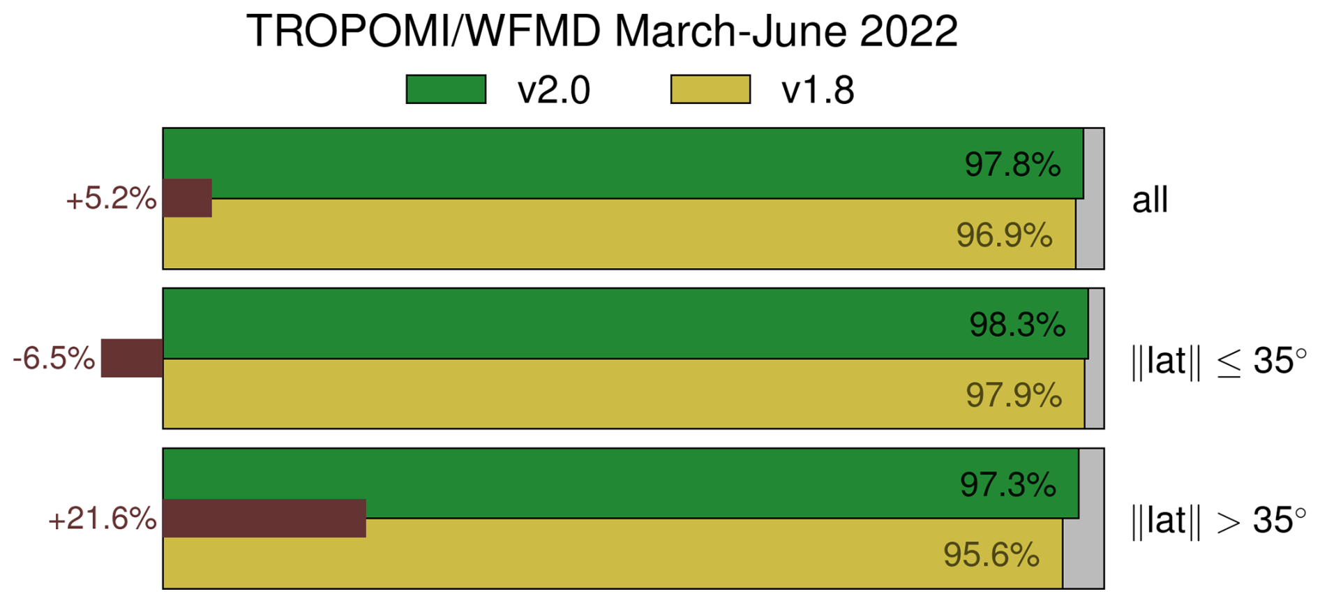
Figure 6 Precision of the quality filter concerning identification of cloud-free scenes in versions 1.8 and 2.0, shown for selected latitude ranges. Precision is defined as the percentage of actually cloud-free scenes according to VIIRS among those passing the quality filter. The brown bars highlight the change in the absolute number of good quality scenes (v2.0 relative to v1.8).

Overall, these results suggest that version 2.0 delivers both improved data quality and increased data yield, except under certain challenging conditions, such as those involving desert aerosols, where somewhat more data is filtered out. However, this observation still needs to be confirmed by validation with independent reference data (see Sect. 3) and a detailed analysis of the regional patterns of the satellite data (see Sect. 4). It needs to be emphasised that the subsequent shallow machine learning calibration, based on a Random Forest Regressor, to reduce the remaining systematic errors in the XCH₄ data remains the same as in v1.8. Specifically, the training regions, the maximum tree growth limit, and the small set of input features, mainly related to albedo, have not been changed. Even though the settings remain identical, this post-processing correction might perform better with the current version as the improved quality filter produces more consistent data, helping the regressor model to learn the core relationships more effectively.

3 Validation

3.1 Random and spatial systematic errors

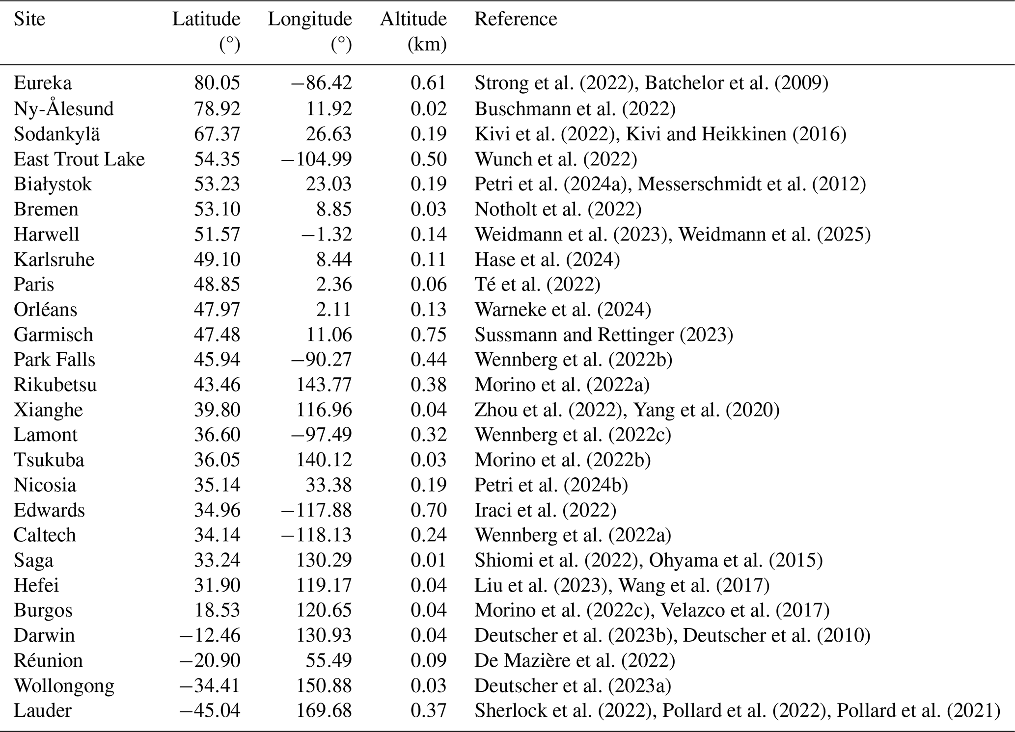
TCCON is a global network of ground-based Fourier-transform spectrometers that measure direct solar radiation in the near- and shortwave-infrared spectral region to retrieve precise column-averaged abundances of trace gases such as XCH₄ and XCO, serving as a benchmark for satellite data validation (Wunch et al., 2011a). All sites operate similar instrumentation (Bruker IFS 125HR) and use a standardised retrieval algorithm. Data are tied to the WMO trace gas scale using airborne in-situ measurements with species-specific scaling factors, yielding estimated accuracies of about 4 ppb for XCH₄ and 2 ppb for XCO in the GGG2020 version used here (Laughner et al., 2024).

To enable a quantitative comparison with satellite data, the differences in instrument sensitivity and prior profiles must be taken into account. This involves adjusting the measurements for the influence of their native prior profiles using a common prior (Rodgers, 2000; Dils et al., 2014; Schneising et al., 2019), here taken from the TCCON:

$$\begin{array}{}\text{(1)}& {\widehat{c}}_{\mathrm{adj}}=\widehat{c}+{\displaystyle \frac{\mathrm{1}}{m_{\mathrm{0}}}}\sum _l{m}_l\left(\mathrm{1}-A_l\right)\left(x_{\mathrm{a},T}^l-x_{\mathrm{a}}^l\right)\end{array}$$

where $\widehat{c}$ is the original TROPOMI retrieval, A_l the satellite averaging kernel, x_a and x_a,T the TROPOMI and TCCON prior profiles, respectively. m_l denotes the dry air mass in layer l from pressure differences corrected for water vapour, and m₀ is the total dry air mass. The averaging kernels of the satellite data product are illustrated in Fig. 7, demonstrating that the retrievals are sensitive to all atmospheric layers.

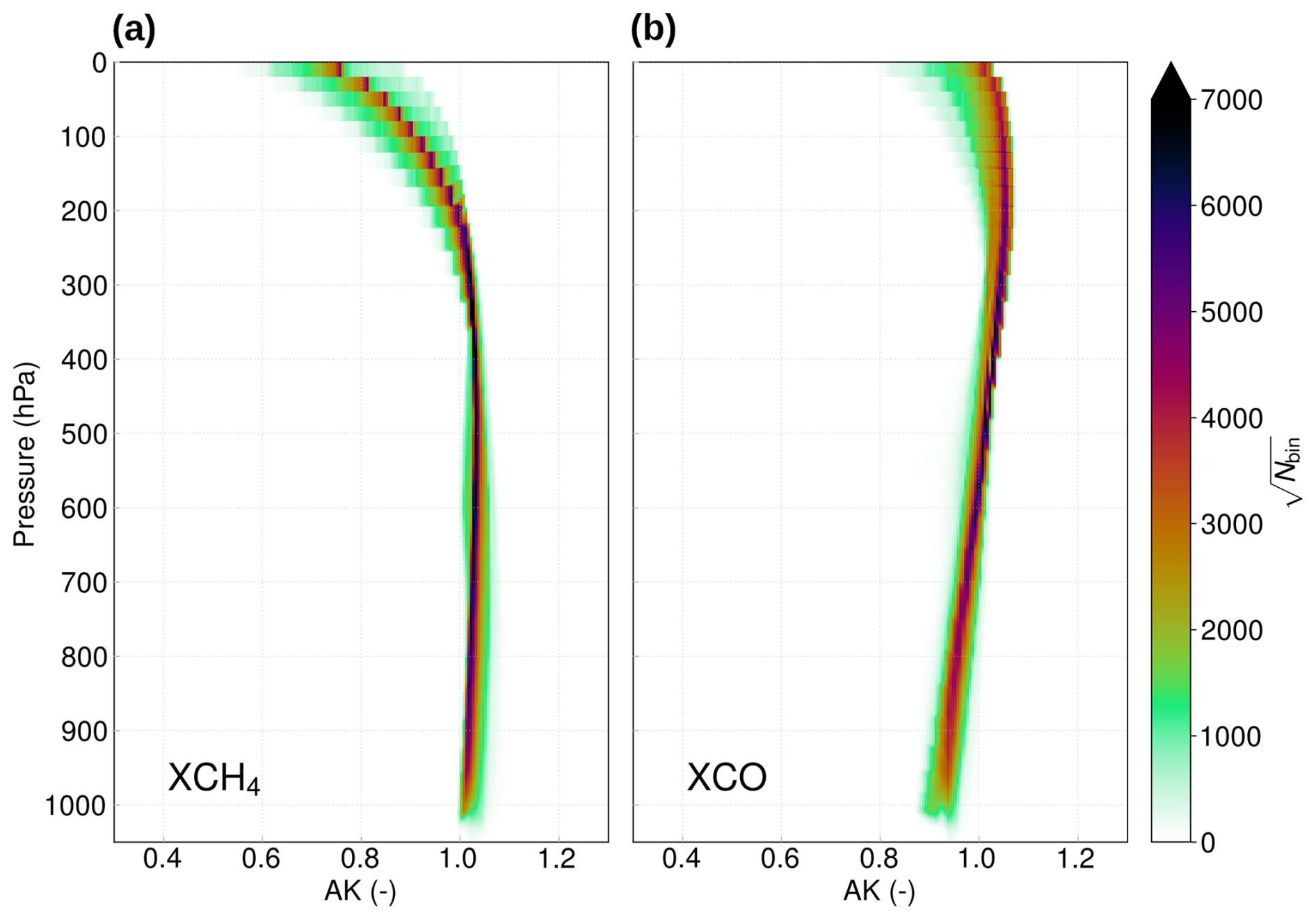
Figure 7 Averaging kernels of the TROPOMI/WFMD v2.0 satellite data product used in the prior profile adjustment of Eq. (1). Shown are the averaging kernels of all measurements from every second day of a given year for (a) XCH₄ and (b) XCO, illustrating the vertical sensitivities of the satellite retrievals.

Theoretically, smoothing errors can be further reduced by adjusting the TCCON results ${\widehat{c}}_T$ before the comparison with ${\widehat{c}}_{\mathrm{adj}}$ using the retrieved TCCON profile scaling factors in conjunction with the satellite averaging kernels (Rodgers and Connor, 2003; Wunch et al., 2011b; Schneising et al., 2019). However, this second correction step is omitted in the present analysis for the sake of simplicity, as it became apparent in the past that this adjustment is negligible in the validation of TROPOMI/WFMD. Since the satellite averaging kernels in the lower atmosphere are sufficiently close to 1.0, the resulting correction would be in the sub-ppb range, which is significantly smaller than the systematic errors associated with the TROPOMI and TCCON retrievals.

To account for surface elevation differences between TROPOMI observations and TCCON measurements, a height correction is applied to the retrieved column-averaged dry-air mole fractions $\widehat{c}$, such that the collocated data pairs are referenced to a common surface pressure (Sha et al., 2021). Specifically, this height correction estimates the mole fraction that would be retrieved by the satellite measurement, had the retrieval been performed at the surface pressure, P_T, of the TCCON station, rather than at the original TROPOMI surface pressure, P. This adjustment incorporates the retrieved TROPOMI profile scaling factor $\widehat{\mathit{\gamma }}$, assuming that the scaling factor does not change but the associated profile x_a is suitably extended or truncated consistent with the updated surface pressure. The complete height-correction is given by

$$\begin{array}{}\text{(2)}& {\widehat{c}}_{P\to P_T}=\left(\widehat{c}\cdot P+\widehat{\mathit{\gamma }}\underset{P}{\overset{P_T}{\int }}{x}_{\mathrm{a}}\left(p\right)\mathrm{d}p\right)P_T^{-\mathrm{1}}\end{array}$$

where the integral accounts for the additional or missing air mass resulting from the difference in surface pressure. The generic prior x_a is available across all realistic pressures and can therefore be applied when P_T>P as well. The integral inherently yields the correct sign depending on whether P or P_T is greater.

The validation is performed using the latest TCCON data version GGG2020 (Laughner et al., 2024) and the 26 sites listed in Table C1. The used collocation criteria balance representativity and statistical robustness: Satellite data must be within 100 km horizontally and 500 m vertically of the TCCON site, with a maximum time difference of 2 h between observations. Since sources in the vicinity of Edwards and Xianghe limit the representability, the collocation radius for these two locations is reduced to 50 km (Schneising et al., 2019).

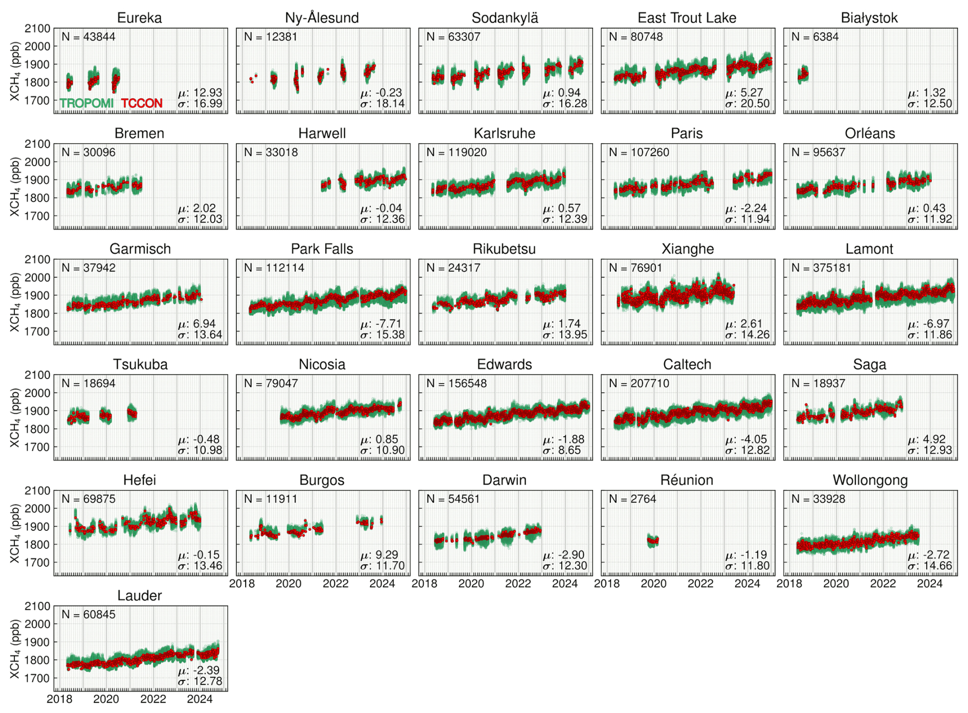
Figure 8 Comparison of the TROPOMI/WFMD v2.0 XCH₄ time series (green) with ground based measurements from the TCCON (red). For each site, N is the number of collocations, μ corresponds to the mean local bias and σ to the scatter of the satellite data relative to TCCON in ppb.

The validation results are summarised in Figs. 8 and 9 including the mean local offsets μ and the scatter σ relative to the TCCON for each site. The results for the individual sites are condensed to the following figures of merit for the overall quality assessment of the satellite data: the global offset $\overline{\mathit{\mu }}$ is defined as the mean of the local biases at the individual sites, the random error $\overline{\mathit{\sigma }}$ is the site-wise mean scatter relative to the TCCON, and the spatial systematic error σ(μ) is the standard deviation of the local offsets relative to the TCCON at the individual sites as a measure of the station-to-station biases. For XCH₄, the global offset amounts to $\overline{\mathit{\mu }}=\mathrm{0.65}$ ppb, the random error is $\overline{\mathit{\sigma }}=\mathrm{13.35}$ ppb, and the spatial systematic error is given by σ(μ)=4.46 ppb. For XCO, the corresponding values are $\overline{\mathit{\mu }}=-\mathrm{0.44}$ ppb, $\overline{\mathit{\sigma }}=\mathrm{5.55}$ ppb, and σ(μ)=2.67 ppb. Thus, the estimated spatial systematic errors for both species are on the order of the estimated (station-to-station) accuracy of the TCCON. In the case of XCH₄, the largest scatter σ relative to TCCON is observed at high northern latitude sites, with the largest local offset μ at Eureka. These features are attributed to the influence of the polar vortex, which can introduce representation errors when the vortex boundary lies between the TCCON site and individual satellite measurements, leading to genuine differences in XCH₄ between the two data sets (Hachmeister et al., 2025).

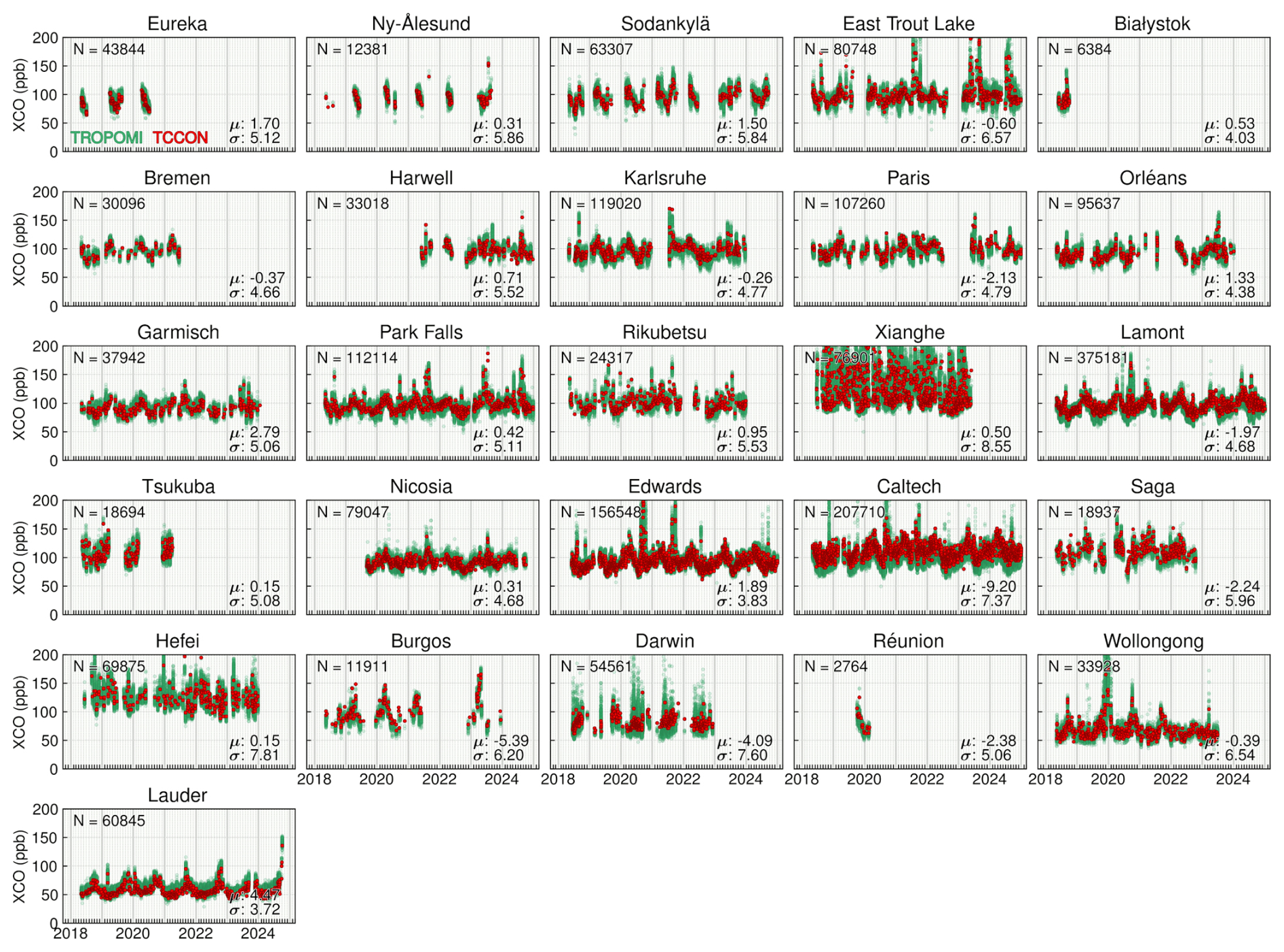
Figure 9 As Fig. 8 but for XCO. Individual collocated pairs with lower agreement are typically associated with wildfire events, e.g., when there is a true XCO enhancement in a distant satellite scene but not directly at the TCCON site or vice versa (representation error).

Figure 10 shows how the validation results compare to the previous version 1.8. Overall, the number of collocations has increased by about 10 % in version 2.0, thanks to better data coverage. In the Arctic in particular, coverage improved by roughly 40 %, which reflects the enhanced data yield under challenging conditions, such as high solar zenith angles and low surface reflectivity. Even though the number of collocations N is larger, which often introduces more variability, both the random and systematic errors have actually improved in v2.0, indicating more consistent and reliable retrievals. The only exception is the spatial systematic XCO error, which remains mostly unchanged. Furthermore, the global offset $\overline{\mathit{\mu }}$ of XCH₄ relative to the TCCON has been significantly reduced and is now nearly zero. While this former global offset was not a critical quality issue since it could be easily corrected with a dedicated bias correction, the fact that it is improved aligns well with the better accuracy of the new v2.0 data product.

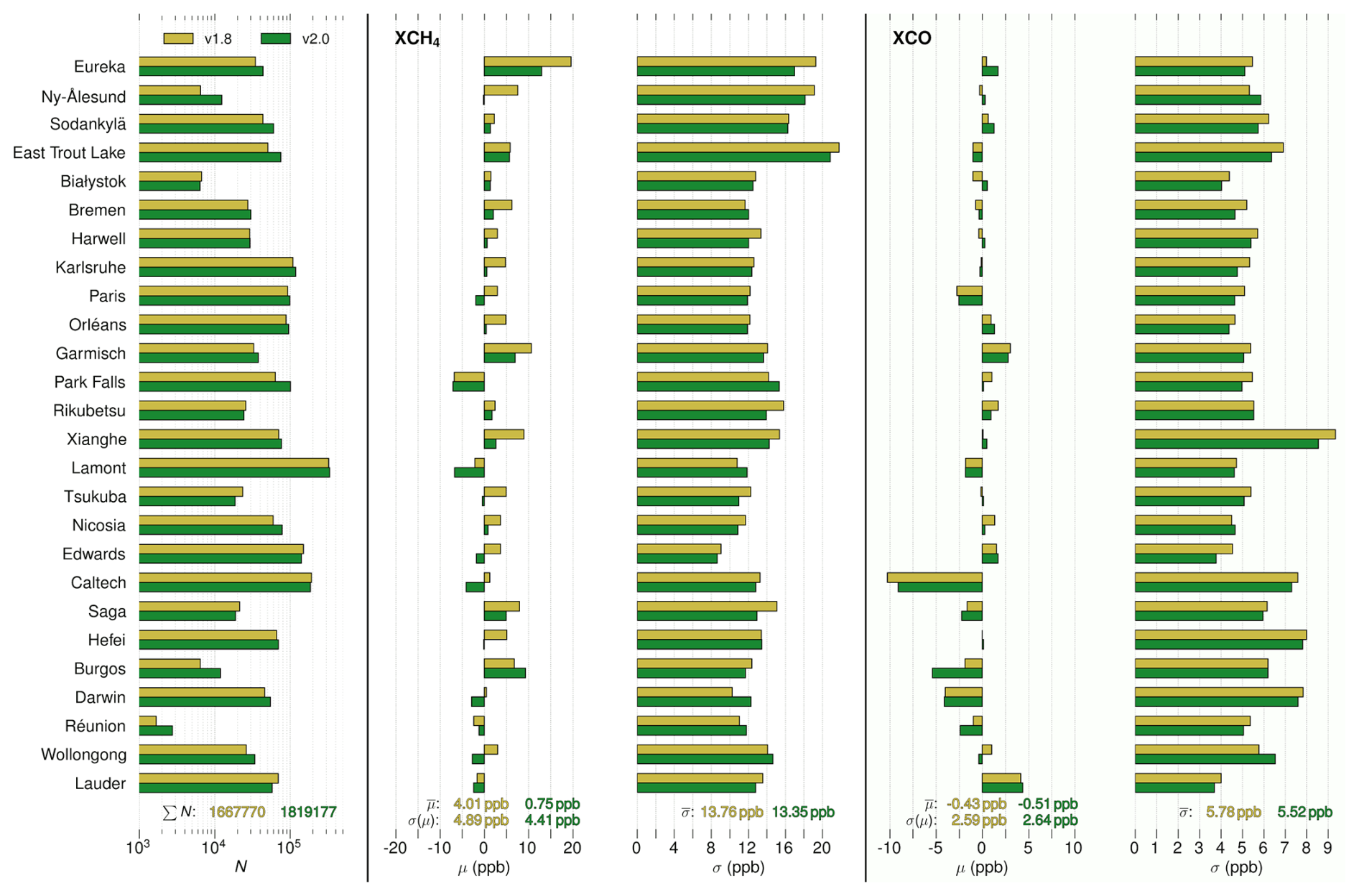
Figure 10 Comparison of the retrieval results for TROPOMI/WFMD v1.8 and v2.0. The comparison was limited to the period during which both product versions were available (May 2018–June 2024). As a result, the numbers differ slightly from those in the full validation of v2.0.

3.2 Seasonal biases

In order to further analyse the intra-annual variability of the discrepancies between the collocated TROPOMI and TCCON data, the site-specific mean offsets μ are first subtracted from the differences of the individual data pairs to remove the already discussed spatial bias component. The resulting anomalies are then grouped by season and categorised as January–March (JFM), April–June (AMJ), July–September (JAS), and October–December (OND). To summarise joint seasonal characteristics, the sites are additionally divided into broad latitudinal bands, namely Arctic (90–66.5° N), Northern mid-latitudes (66.5–23.5° N), Tropics (23.5–23.5° S), and Southern mid-latitudes (23.5–66.5° S). Since there are many TCCON sites in the Northern Hemisphere's mid-latitudes, this band is further separated into smaller sub-regions based on longitude (North America, Europe, and Asia). The associated spatio-temporal averages are only included in the analysis for those combinations of region and season that contain data from at least three different years for more than one calendar month of the respective season in order to ensure statistical robustness.

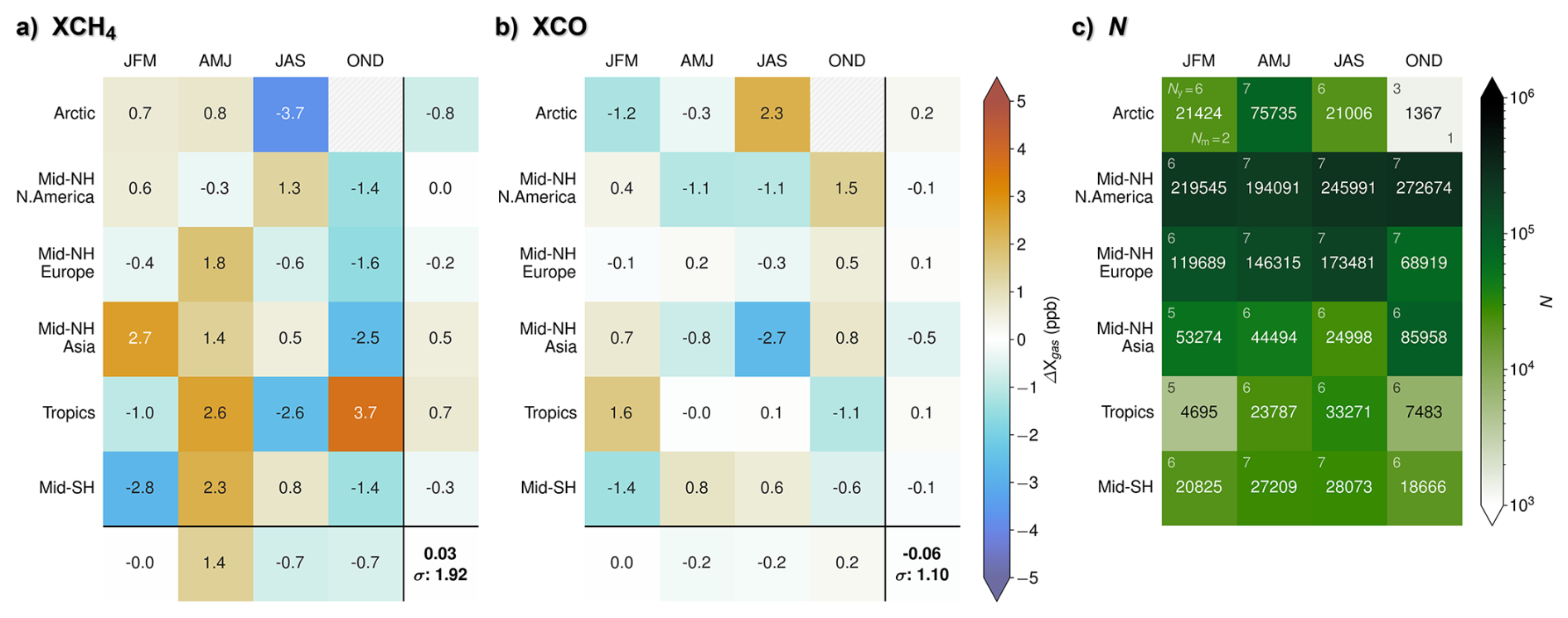
Figure 11 Seasonal mean biases for (a) XCH₄ and (b) XCO relative to the TCCON for the analysed regions. Masked cells indicate insufficient coverage (see main text for details). Row and column averages further summarise the overarching regional and seasonal variability. The standard deviation of the seasonal biases across all regions is interpreted as the overall seasonal bias and indicated in the bottom-right corner. (c) Number of collocations N for the different combinations of region and season. The number of contributing years N_y is shown in the top-left corner of each cell; the number of calendar months N_m contributing data to the corresponding 3-month season is displayed in the bottom-right corner of each cell, only if it is smaller than the maximum value of 3.

The results are displayed as heat maps in Fig. 11, where the average bias values are annotated on the corresponding cells and entries with insufficient sampling are masked. In addition, the row and column mean values provide an average overview of regional and seasonal variations, respectively. The total seasonal bias relative to the TCCON is then calculated as the standard deviation of the individual biases across all regions and seasons, resulting in 1.92 ppb for XCH₄ and 1.10 ppb for XCO.

3.3 Uncertainties

The individual uncertainties of the TROPOMI/WFMD measurements are provisionally estimated during the inversion process by error propagation based on the uncorrelated spectral errors provided in the TROPOMI Level 1 files. However, this estimate does not take into account pseudo-noise components that may arise from specific atmospheric conditions or instrumental characteristics, nor systematic uncertainties associated with spectroscopic parameters. For this reason, the initial uncertainty estimates tend to underestimate the actual measurement error and are therefore inflated by a simple linear adjustment to provide more realistic values (Schneising, 2025).

The resulting final uncertainties σ_unc reported in the TROPOMI/WFMD v2.0 product are checked by comparison with the actual measured scatter relative to the TCCON. To this end, a data-driven adaptive binning approach based on k-means$++$ clustering (Arthur and Vassilvitskii, 2007) is applied as a preparatory step. This approach divides the data into discrete bins of similar uncertainty by minimising the within-cluster variance. For each of these bins, the mean reported uncertainty is calculated and compared to the actual observed scatter of the differences relative to the TCCON. The results presented in Fig. 10 demonstrate that the uncertainty estimates provided are generally realistic, as evidenced by the fact that the mean uncertainty ratio $\overline{\mathrm{\Gamma }}$, defined as the reported uncertainty divided by the measured scatter, is close to 1.0 (1.03 for XCH₄ and 1.01 for XCO), which is what one would expect from a reliable, high-quality uncertainty estimate. There is a slight overall tendency to overestimate the uncertainties on average ($\overline{\mathrm{\Gamma }}>\mathrm{1}$), with the exception of the rather rare cases of poor XCO precision, where the reported uncertainties of the satellite data appear to be somewhat underestimated.

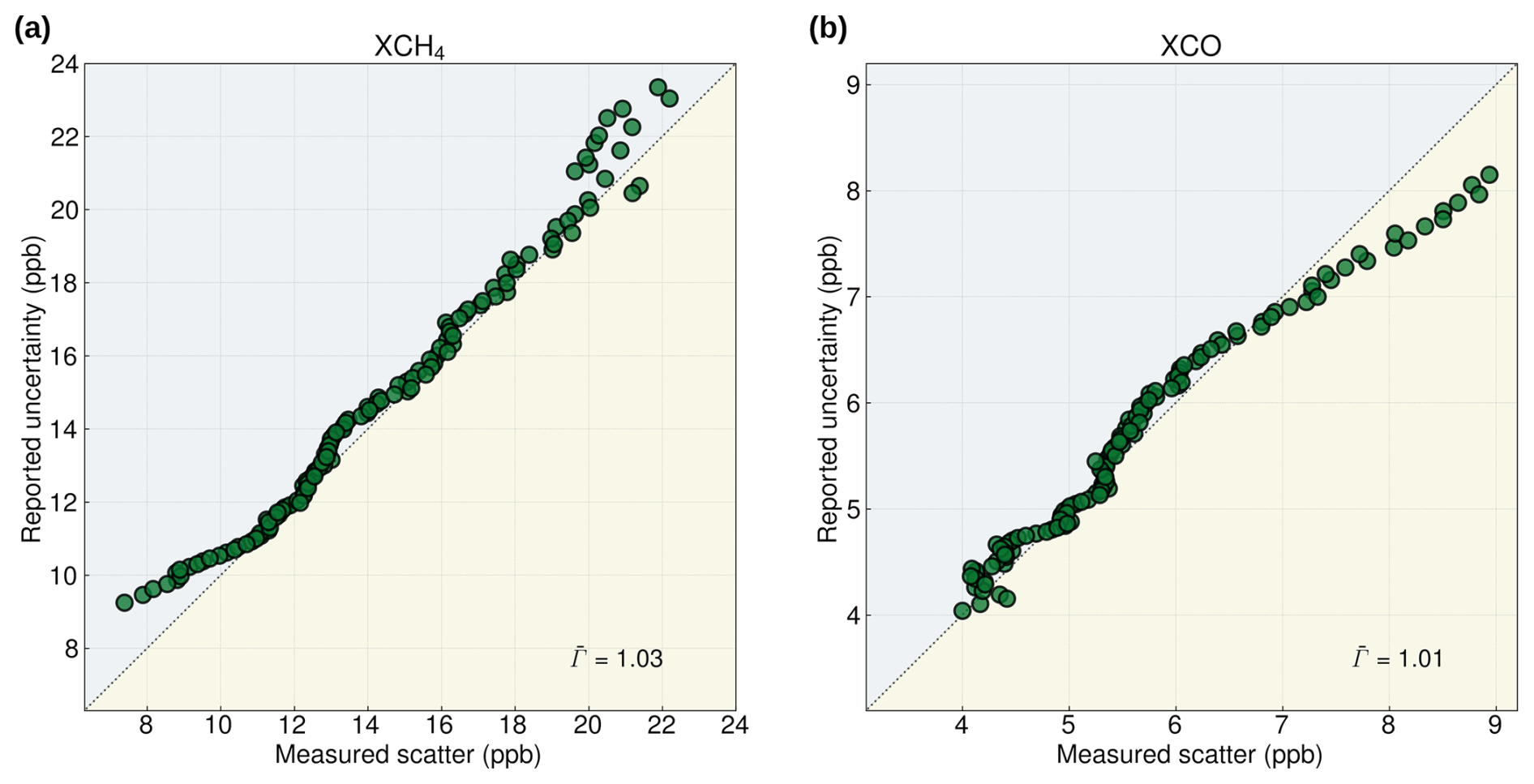
Figure 12 Comparison of reported uncertainties in the TROPOMI/WFMD v2.0 product with the measured scatter relative to the TCCON for (a) XCH₄ and (b) XCO. In the blue-shaded areas, reported uncertainties exceed the observed scatter (overestimation), whereas in the yellow-shaded areas, they fall below it (underestimation).

3.4 Surface albedo sensitivity

To investigate possible albedo-related biases in the TROPOMI/WFMD product, the sensitivity of TROPOMI to TCCON discrepancies with respect to surface albedo variability is examined on a daily basis, taking into account site-specific offsets that could complicate the determination of such a relationship. Although the local offsets determined during the validation are probably largely independent of albedo, it cannot be entirely excluded that albedo also contributes to some extent to the site-specific biases. To rigorously account for this by disentangling these components, a joint hierarchical Bayesian linear regression model from the probabilistic programming library PyMC (Abril-Pla et al., 2023) is applied, which allows comprehensive uncertainty quantification and propagation, enabling a fully probabilistic characterisation of albedo sensitivity. In this framework, site-specific offsets are modelled as random intercepts informed by the previous validation results, while the relationship between surface albedo and the difference to the TCCON is represented by a global fixed regression slope β across all sites. Consequently, the hierarchical approach leaves the model free to attribute parts of the estimated local biases to albedo, thus yielding a more realistic estimate of β.

The model inference is performed by Markov Chain Monte Carlo sampling using the No-U-Turn Sampler (NUTS), an adaptive Hamiltonian Monte Carlo algorithm that efficiently explores high-dimensional posterior distributions, even in the presence of complex hierarchical structures. In the specific case presented here, six independent chains are run in parallel and their convergence to a common posterior distribution is evaluated using the potential scale reduction factor $\widehat{R}$ (Vehtari et al., 2021), which compares the variance between multiple chains to the within-chain variance. Values of $\widehat{R}$ close to 1.0 indicate that the chains have mixed well, i.e., they have sufficiently explored the parameter space and converged to virtually the same posterior distribution.

To inform plausible data-driven values for the slope parameter β, the observed albedo range is divided into bins of fixed width. Within each bin, the median values of albedo, ΔXCH₄ and ΔXCO (satellite minus collocated TCCON measurements) are calculated, and the respective slopes for all possible pairs of bins are computed to obtain an empirical distribution that reflects the variability over the entire domain. The median absolute deviation (MAD) of these pairwise slopes is then used to conservatively estimate the variability σ_β. Assuming a normal prior centered at zero, this defines a weakly informative normal prior for the slope parameter β.

With i denoting individual daily averaged observations and j indexing TCCON sites, the complete hierarchical model includes hyperpriors on site-level intercepts, additional informative validation-based anchor data, a linear predictor combining site biases and albedo dependence, and a likelihood assuming normally distributed observational uncertainties:

$$\begin{array}{}\text{(3)}& \begin{array}{lll}{a}_j\sim \mathcal{N}({\mathit{\mu }}_a,{\mathit{\sigma }}_a)& \text{with}& {\mathit{\mu }}_a\sim \mathcal{N}(\overline{\mathit{\mu }},\mathit{\sigma }(\mathit{\mu }\left)\right)\\ & & {\mathit{\sigma }}_a\sim \mathcal{H}\mathcal{N}\left(\mathit{\sigma }\right(\mathit{\mu }\left)\right)\\ {\widehat{a}}_j\sim \mathcal{N}(a_j,{\mathit{\sigma }}_{\text{eff},j})& \text{with}& {\mathit{\sigma }}_{\text{eff},j}=\frac{{\mathit{\sigma }}_j}{\sqrt{f{N}_j}}\\ & & f\sim \mathcal{B}(\mathrm{2},\mathrm{2})\\ {\mathit{\xi }}_i=a_{j\left[i\right]}+\mathit{\beta }{\mathit{\alpha }}_i& \text{with}& \mathit{\beta }\sim \mathcal{N}(\mathrm{0},{\mathit{\sigma }}_{\mathit{\beta }})\\ {\mathrm{\Delta }}_i\sim \mathcal{N}({\mathit{\xi }}_i,{\mathit{\sigma }}_{\text{obs},i})& \text{with}& {\mathit{\sigma }}_{\text{obs},i}^{\mathrm{2}}={\mathit{\sigma }}_{\text{unc},i}^{\mathrm{2}}+{\mathit{\sigma }}_{\text{res},j\left[i\right]}^{\mathrm{2}}\\ & & {\mathit{\sigma }}_{\text{res},j\left[i\right]}\sim \mathcal{H}\mathcal{N}\left(\frac{\mathrm{1}}{\mathrm{2}}{\overline{\mathit{\sigma }}}_{\text{unc}}\right)\end{array}\end{array}$$

where 𝒩 denotes a normal distribution, ℋ𝒩 denotes a half-normal distribution, and ℬ a Beta distribution. The systematic errors $\overline{\mathit{\mu }}$ and σ(μ) estimated from the preceding validation are used to construct the prior for a_j, which describes the site-specific bias for site j. The local biases are further informed by observed validation-based estimates ${\widehat{a}}_j$, which are treated as noisy measurements with effective standard errors σ_eff,j reflecting the corresponding uncertainties of the previously obtained local offset estimates μ_j from validation. Thereby, the co-fitted factor $f\in (\mathrm{0},\mathrm{1})$ shrinks the collocation sample size N_j in computing the standard error from the scatter σ_j relative to the TCCON. The parameters μ_j, σ_j, and N_j are defined as in Figs. 8 and 9 but for daily averages. The quantity ξ_i is the mean response predicted by the model for observation i (where j[i] refers to the site associated with i), α_i denotes the associated surface albedo, and Δ_i are the observed differences to TCCON, incorporating both the daily averaged reported observational uncertainty σ_unc,i (see previous subsection) and site-level residual variability σ_res,j[i]. The additional σ_res may be elevated at specific sites, for example due to representation errors during wildfire events, when for some Δ_i the two involved data sets are differently affected by corresponding XCO enhancements as a result of spatial separation.

In Fig. 13, the posterior mean values of the site-specific intercepts a_j have been subtracted from the observed ΔXCH₄ and ΔXCO values to focus on their dependence on surface albedo. The resulting residuals are free of site-to-site biases and are thus ideally suited to analyse the pure albedo sensitivity β of the data. The arising marginal posterior distributions of the albedo sensitivity parameter are shown as insets in the figure together with the results of the individual Markov Chains. The excellent agreement between the individual resulting distributions, with an associated potential scale reduction factor ${\widehat{R}}_{\mathit{\beta }}$ close to 1.0 in both cases, demonstrates that the sampling chains have reliably converged to a common posterior distribution.

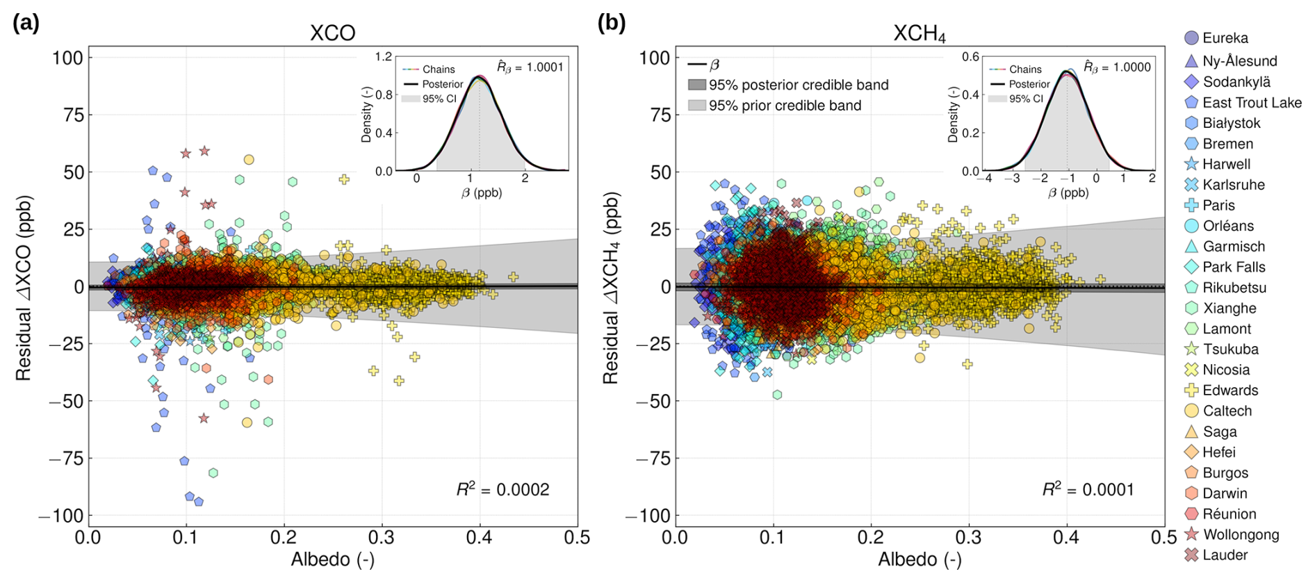
Figure 13 Assessment of the surface albedo sensitivity of TROPOMI/WFMD v2.0 (a) XCO and (b) XCH₄ based on daily means. Residual ΔXCO and ΔXCH₄ were obtained by subtracting the posterior mean site-specific intercepts from the observed differences to remove site-to-site biases. The fitted slope β and its 95 % credible band are overlaid illustrating the inferred sensitivity to surface albedo for each trace gas. The insets show the respective marginal posterior distribution of the albedo sensitivity parameter β from the hierarchical model. The width of the distribution reflects the inferred uncertainty in the slope, with the peak indicating the most probable value.

The found surface albedo sensitivity in the case of XCO is $\mathit{\beta }=\mathrm{1.2}\pm \mathrm{0.8}$ ppb for a unit increase in albedo (Δα=1), with a coefficient of determination R²=0.0002. This means that there is a statistically significant positive relationship between surface albedo and ΔXCO, but albedo explains only a marginal fraction of the overall variance. Some additional uncertainty arises from the fact that the TCCON collocations may not fully represent the entire range of naturally occurring surface albedos. For XCH₄, the estimated sensitivity is $\mathit{\beta }=-\mathrm{1.1}\pm \mathrm{1.5}$ ppb per unit albedo, with R²=0.0001 suggesting that there is no significant bias due to surface albedo. If we consider only the two neighbouring sites, Edwards and Caltech, whose combined albedo range already extends from 0.1 to 0.4, the sensitivities for both gases are very similar to those obtained in the full analysis, albeit with increased uncertainty. Since albedo is a dimensionless quantity with values ranging from 0 to 1, and typical observed albedo values cover a considerably narrower subrange, the practical influence of surface albedo on XCO and XCH₄ is correspondingly even smaller. Thus, the albedo-induced bias under typical conditions is limited to the sub-ppb range. These results imply that surface albedo has a minor impact on the XCO retrievals and a negligible effect on XCH₄ in terms of retrieval biases.

Because the albedo range covered by the TCCON comparison is limited (α≲0.4), an additional analysis independent of the TCCON is performed to further assess albedo sensitivity. In the absence of a reference data set to serve as ground truth, a region with negligible methane emissions has to be selected. For this reason, the Sahara is used here (see Fig. 14), which also has high albedo variability and is therefore well-suited for this analysis. To remove the influence of the seasonal cycle and the long-term methane increase, the seasonal and level components of a Dynamic Linear Model (DLM) (Hachmeister et al., 2024) based on daily data are subtracted from the time series of individual satellite observations, yielding an anomaly ΔX_gas for each measurement. The albedo sensitivity is then estimated as the slope parameter β of a linear regression fit between these anomalies and surface albedo. To assess uncertainty, we use a subsampling bootstrap technique, in which random subsets of 1000 data points are repeatedly drawn from the complete data set and linear regression is re-performed on each subset. This yields empirical distributions of the regression parameters, from which uncertainties are quantified using the corresponding 95 % credible bands.

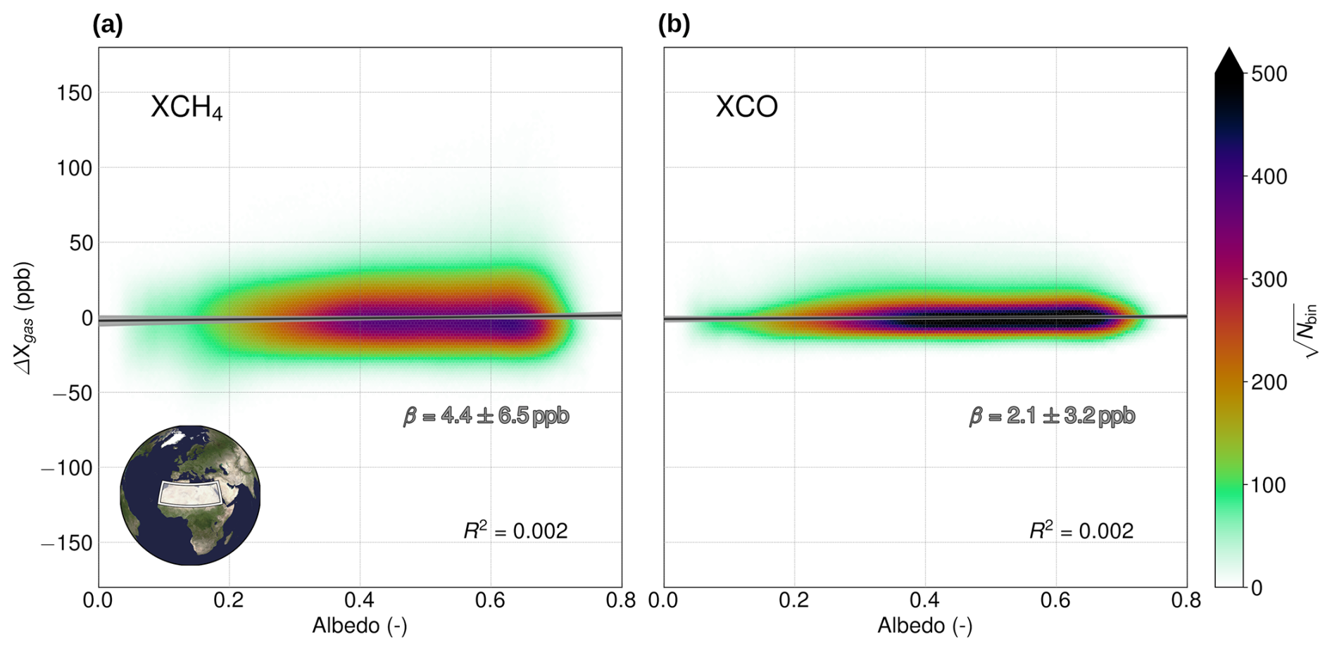
Figure 14 Assessment of the surface albedo sensitivity of TROPOMI/WFMD v2.0 over the Sahara (white region) for (a) XCH₄ and (b) XCO after subtracting the seasonal and level components of a fitted Dynamic Linear Model (DLM). The fitted slope β and its 95 % credible band are overlaid illustrating the inferred sensitivity to surface albedo for each trace gas.

The findings align with the TCCON-based results and show that there is no evidence of critical albedo-related biases in the TROPOMI/WFMD data. In fact, the estimated surface albedo sensitivities β are of the same order of magnitude as in the TCCON assessment and do not differ significantly from zero. The magnitude of the uncertainty estimates is about four times greater than that of the TCCON analysis. Specifically, the sensitivities are $\mathit{\beta }=\mathrm{4.4}\pm \mathrm{6.5}$ ppb per unit albedo for XCH₄ and $\mathit{\beta }=\mathrm{2.1}\pm \mathrm{3.2}$ ppb for XCO, with a coefficient of determination of R²=0.002 in both cases.

3.5 Summary of validation results

Independent ground-based measurements from the TCCON confirmed that the updated TROPOMI/WFMD v2.0 XCH₄ and XCO products have higher quality than the previous version. The refined retrievals are not only more accurate and precise, but also provide increased data yield at mid and high latitudes, including observationally challenging regions such as the Arctic. The broader coverage of v2.0 is beneficial for all types of applications, whether at the regional level, such as quantifying local hotspot emissions, or on a larger scale, like analysing growth rates of latitude bands. According to the review of the uncertainties reported for each measurement, the estimates are reasonable and realistic. Furthermore, the analysis showed that surface albedo does not introduce any relevant biases into the data products. This is an important finding as albedo-related biases are often a concern in the application of TROPOMI methane retrievals (Barré et al., 2021; Balasus et al., 2023).

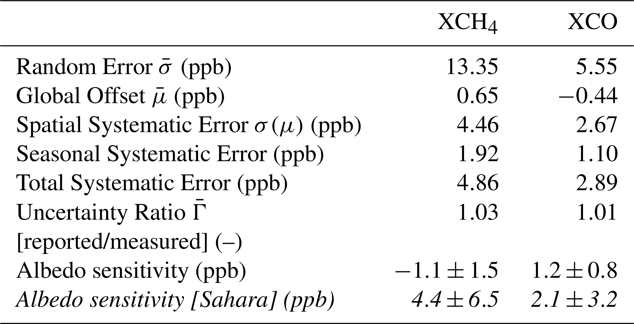
The improved performance relative to the previous version is driven primarily by the updated quality filtering, whereas the additional processing changes have only a minor effect in comparison. The quality assessment results are summarised in Table 2, including metrics that measure both random and systematic errors of the data product. These figures of merit give a clear overview of how well the TROPOMI/WFMD v2.0 products perform and are helpful benchmarks for users intending to use the data in scientific research. The reported values should be interpreted as upper limits, reflecting uncertainties in the TCCON reference as well as potential representation errors arising from the non-zero collocation radius, particularly when one instrument is affected by local events such as wildfires or the polar vortex and the other is not.

Table 2 Figures of merit from the quality assessment of TROPOMI/WFMD v2.0 using TCCON GGG2020. The total systematic error is defined as the root-sum-square of the spatial and seasonal systematic errors. Also shown is the derived albedo sensitivity from the TCCON-independent time series analysis over the Sahara in italics.

Overall, the TROPOMI/WFMD v2.0 product performs reliably in retrieving XCH₄ and XCO from actual TROPOMI data, achieving accuracy and precision levels well within the mission requirements after appropriate quality filtering. In concrete terms, this means that the products meet the strict limits of less than 1.5 % bias and 1.0 % random error for XCH₄, as well as less than 15 % bias and 10 % random error for XCO, confirming the suitability of the algorithm for quasi-operational processing of TROPOMI measurements.

4 Regional assessments

To elucidate how the improvements in TROPOMI/WFMD v2.0 manifest in the retrieval results, this section examines regional patterns in the data products. While previous sections focussed on evaluating the trained quality filter using unseen data and validation with independent reference measurements from the TCCON, the spatially resolved assessment here reveals how these refinements translate specifically into increased regional coverage. While this section mainly discusses XCH₄ because of its stricter quality requirements, it is worth noting that the data coverage for XCO is exactly the same across all cases. Depending on the intended application, this assessment is carried out by means of selected examples based on temporal averaging on a ${\mathrm{0.1}}^{\circ }\times {\mathrm{0.1}}^{\circ }$ grid or daily swath data.

As a first step, Fig. 15 presents the global distribution of the retrieved XCH₄ and XCO mole fractions for the years 2022 and 2023. There are clear differences between the hemispheres with higher values in the Northern Hemisphere, where most emission sources are concentrated. This gradient is further modified by additional increases over key regions, such as China, India, and Southeast Asia, which are caused by the many anthropogenic sources located there. For XCH₄, elevated abundances are also observed over tropical wetlands and specific hotspots, such as California's Central Valley and the Po Valley in northern Italy. For XCO, additional enhanced values are primarily associated with biomass burning in Africa and South America, as well as with major urban agglomerations including Mexico City and Tehran. The coverage over land is generally high, although persistent cloud cover and low surface reflectivity result in some data gaps near the equator. Coverage over oceans and inland waters is more limited, as good measurements mainly occur under favourable observational conditions, such as sun-glint geometries or certain sea ice scenarios.

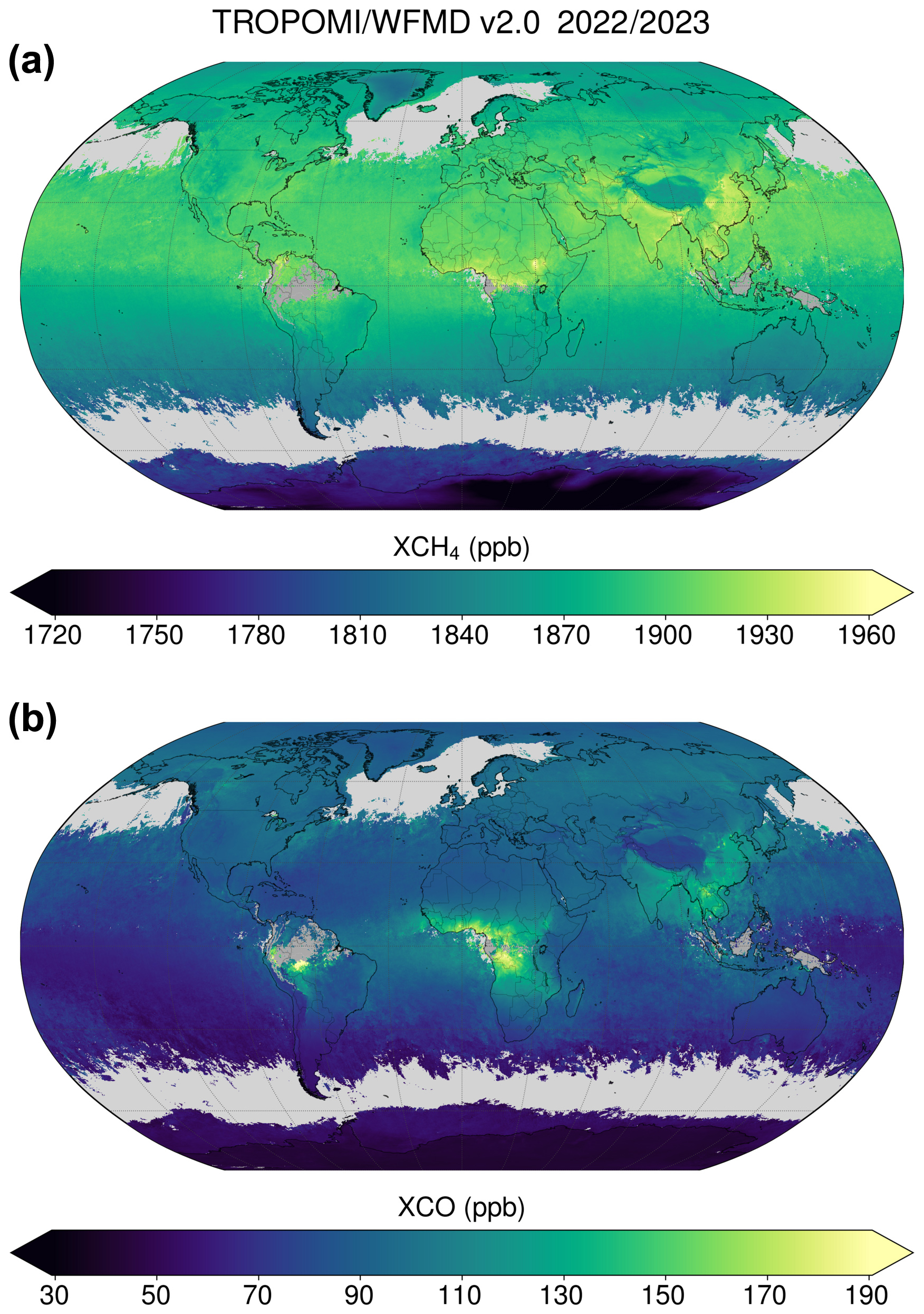
Figure 15 Biennial mean (2022/2023) of retrieved TROPOMI/WFMD v2.0 (a) XCH₄ and (b) XCO.

To further assess the performance of the updated quality filter, regional coverage and temporal variability are analysed using monthly data. Figures 16 and 17 present the differences between v1.8 and v2.0 for February and October 2023. An obvious change in v2.0 is the slight decrease in coverage over the Sahara, attributable to stricter aerosol filtering. Conversely, coverage at higher latitudes has improved, in line with the results of Sect. 3. For a given grid cell, v2.0 shows less variation within a month, especially in desert and mountain areas, which is reflected in reduced scatter σ. While the standard deviation for each grid cell partly captures natural changes, the overall reduction indicates that more low-quality observations have been filtered out.

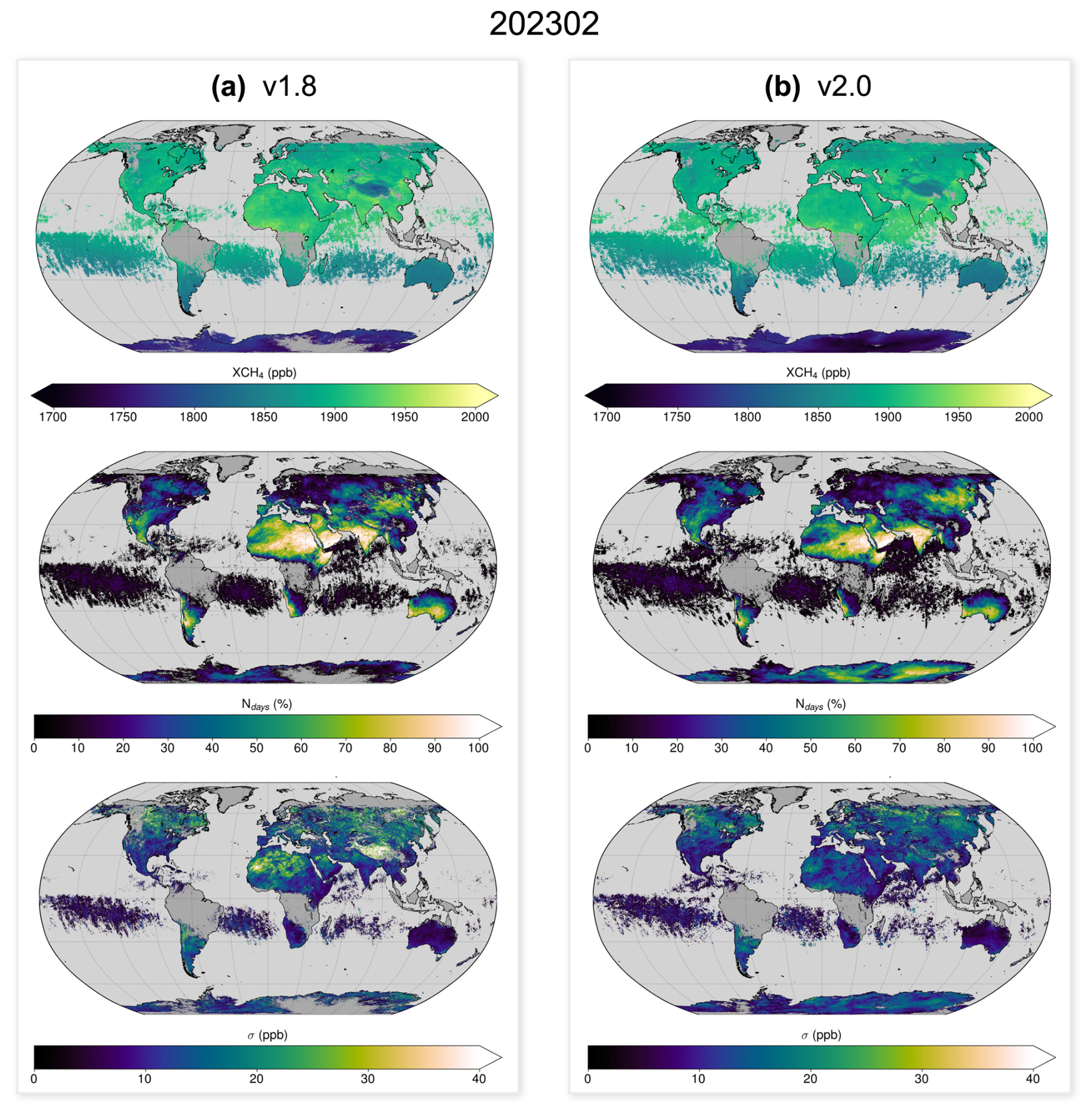
Figure 16 Comparison of monthly averages for (a) TROPOMI/WFMD v1.8 and (b) v2.0 using the example of February 2023. The top row shows the XCH₄, the middle row the number of days that contribute to the monthly average as a percentage (100 % corresponds to 28 d in this example), and the bottom row the standard deviation of XCH₄ per grid cell. As at least two values are required to calculate a meaningful standard deviation, only grid cells with two or more measurements are shown in the bottom row.

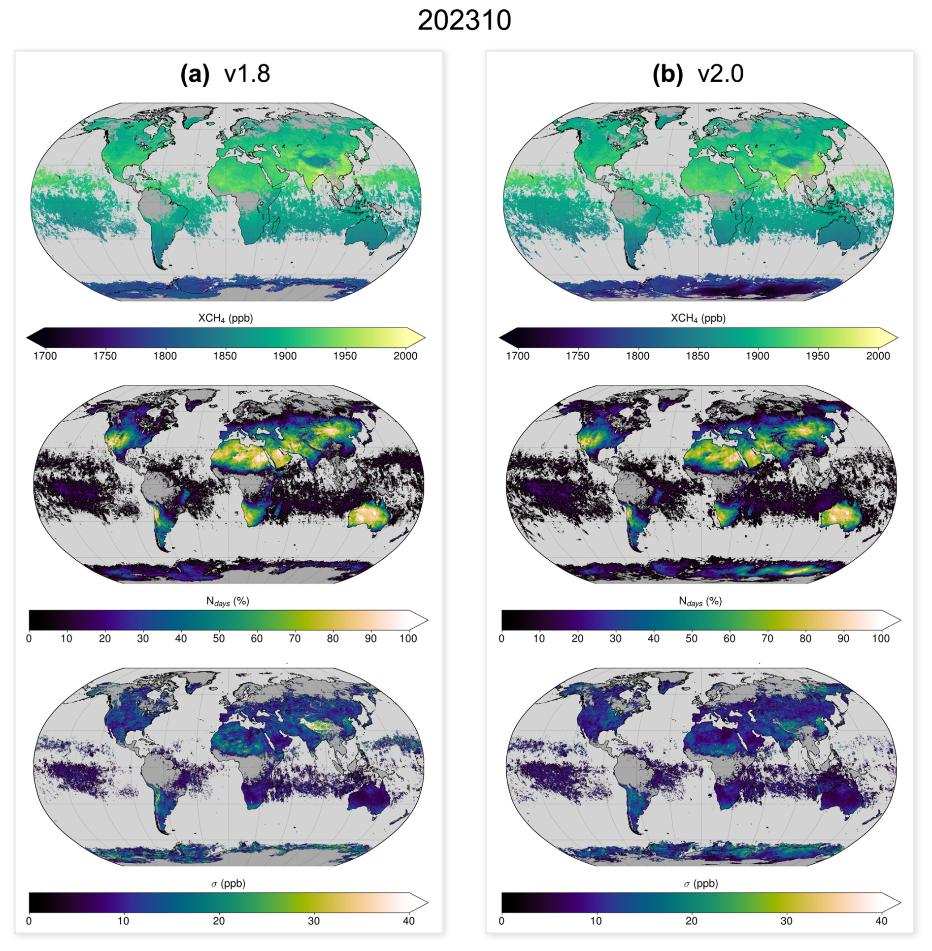
Figure 17 As Fig. 16 but for October 2023.

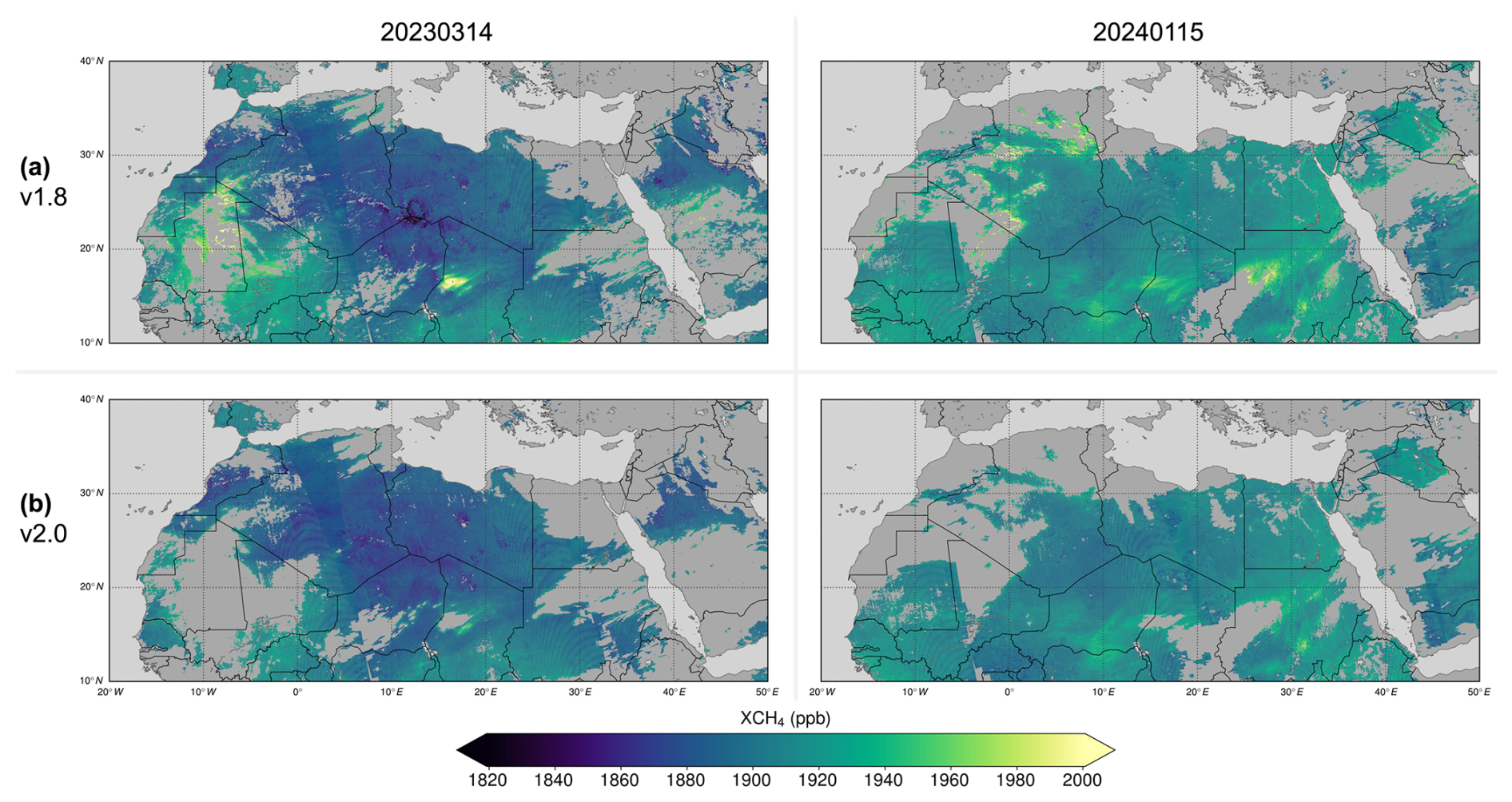
Figure 18 Comparison of (a) TROPOMI/WFMD v1.8 and (b) v2.0 XCH₄ for two example days (columns) over the Sahara demonstrating the improved filtering of spurious high values associated with individual aerosol events or cloud edges in v2.0.

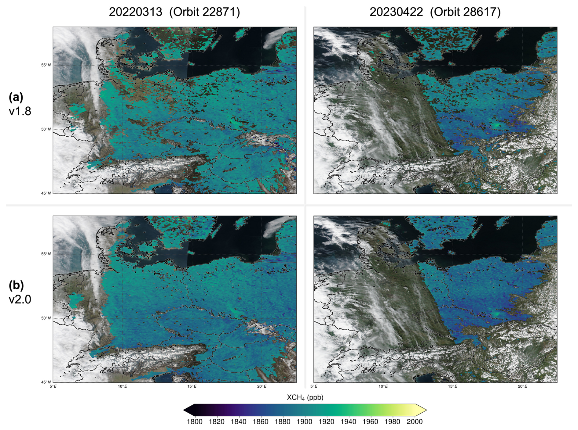
Figure 19 Comparison of (a) TROPOMI/WFMD v1.8 and (b) v2.0 XCH₄ over Central Europe for example satellite overpasses demonstrating the improved cloud screening in v2.0. The background shows the corresponding Suomi NPP/VIIRS True Colour image (bands I1-M4-M3) to highlight the position of the clouds. Elevated methane abundances associated with emissions from the Upper Silesian Coal Basin in Poland are clearly visible on both days.

In addition to temporally averaged products, individual Level 2 swath data help evaluate how the updated quality filter performs under specific atmospheric conditions, such as dust storm events over the Sahara. Figure 18 shows two example days where the v2.0 filter more effectively removes aerosol-contaminated observations than v1.8. In these cases, the number of retained observations in v2.0 is reduced by 19 % and 12 %, respectively. In particular, spurious high values linked to elevated aerosol loading or cloud edges are removed more reliably, e.g., those from dust plumes originating from the Bodélé Depression in Chad. The result is a much more spatially homogeneous methane distribution in v2.0 compared to v1.8.

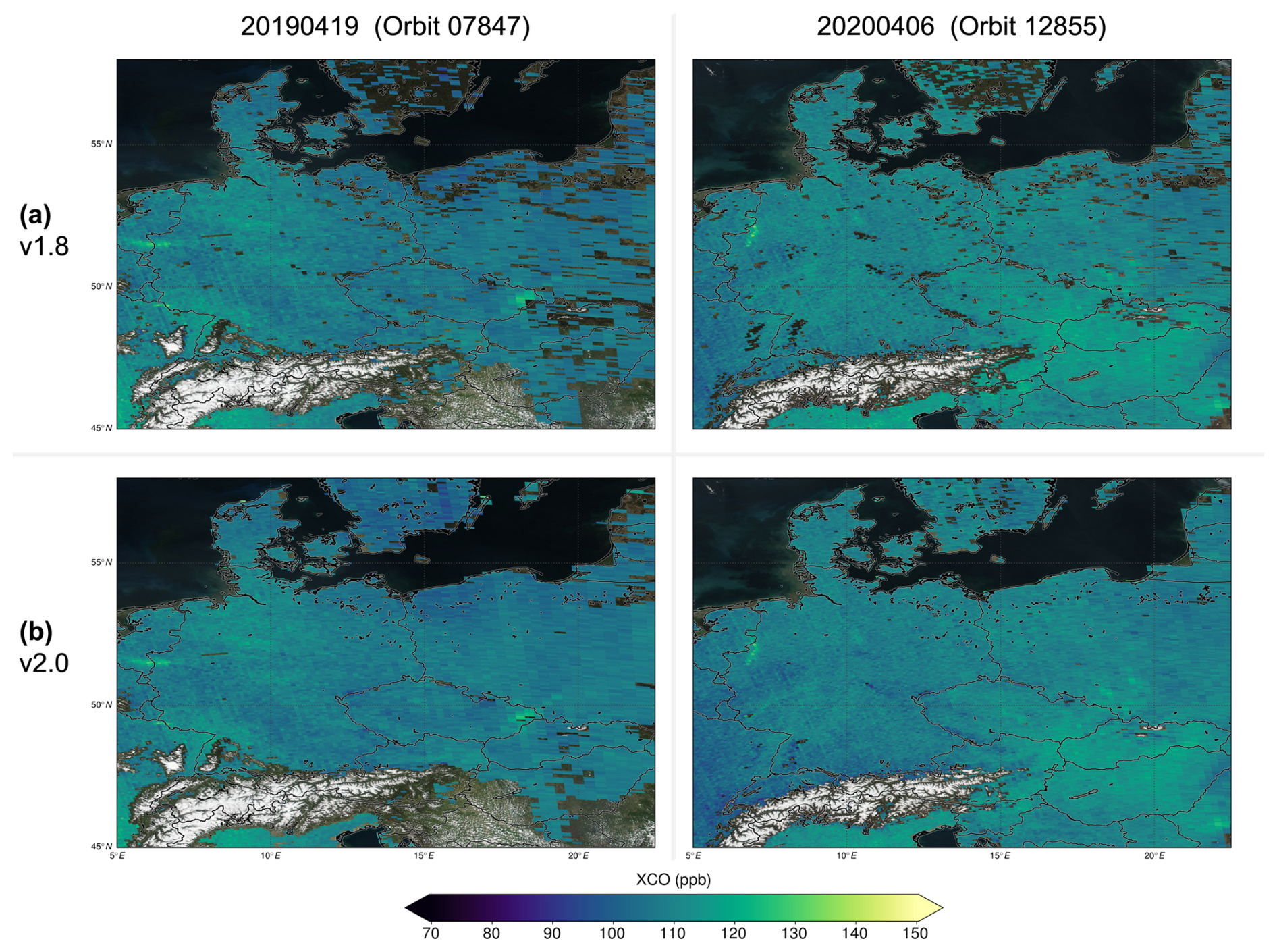
Figure 20 Similar to Fig. 19 but showing XCO and different satellite overpasses. Distinct enhancements are evident over major Central European steelworks including those located in Duisburg and Dillingen, Germany.

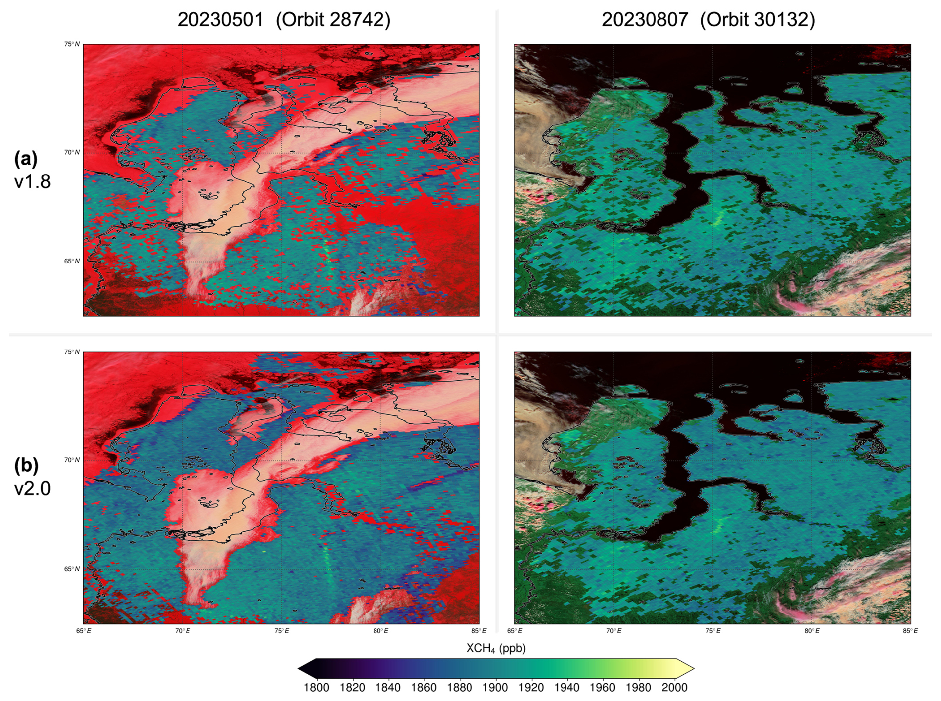
Figure 21 Comparison of (a) TROPOMI/WFMD v1.8 and (b) v2.0 XCH₄ over Siberia for example satellite overpasses demonstrating the improved cloud screening in v2.0. The background shows a specific Suomi NPP/VIIRS false-colour composite (bands M3-I3-M11), which is capable of distinguishing clouds (warm off-white) from snow/ice (bright red). In a true colour image both would appear white and would be indistinguishable. The observed elevated methane abundances are attributed to leakage from oil and gas facilities.

The v2.0 quality filter also improves cloud screening and increases data coverage at mid- and high latitudes. Figures 19–21 show example satellite overpasses over Central Europe and Siberia for both XCH₄ and XCO. While both versions correlate well and effectively remove cloudy scenes, v2.0 allows more valid observations under cloud-free conditions, thereby boosting the data yield. In these examples, the number of soundings passing the filter increases by about 10 %–20 % over Central Europe, and by 60 % and 15 % for the two example overpasses in Siberia. Better coverage also enables improved estimation of emissions sources, some examples of which are easily identifiable in the presented images. In Fig. 19, methane emissions from the Upper Silesian Coal Basin in Poland are evident on both observation days, while the Siberian enhancements in Fig. 21 are associated with methane leakage from oil and gas infrastructure. Figure 20 displays major carbon monoxide emissions from steel production plants in Central Europe, particularly in Germany, Poland, Slovakia, and the Czech Republic (Schneising et al., 2024; Leguijt et al., 2025).

These figures use various Suomi NPP/VIIRS band combinations to highlight cloud cover, which helps to visually identify observations that should be excluded. In the examples for Central Europe, the background image displays a True Colour composite (bands I1-M4-M3), which closely resembles the natural appearance of land, ocean, and atmospheric features as perceived by the human eye. In this representation, the clouds appear white due to the approximately equal scattering of light across the visible bands used.

For the Siberian case, a false-colour composite (bands M3-I3-M11) is used instead, because it more effectively distinguishes clouds from snow and ice, which look similar in standard true-colour images. In this representation, snow and ice appear bright red because they strongly reflect visible light (band M3, centered at 0.49 µm), while they strongly absorb in the shortwave infrared (SWIR) range (band I3: 1.61 µm; band M11: 2.25 µm). Vegetation appears green as it reflects strongly in band I3 but much less in the other two bands. Water clouds are warm off-white with a pale orange or beige tint, while high cirrus clouds appear pastel pink as a result of scattering by small ice crystals.

5 Conclusions

The TROPOMI/WFMD v2.0 product represents a substantial advance in the remote sensing of atmospheric XCH₄ and XCO from space. This improvement is mainly the result of implementing refined quality filtering based on Extreme Gradient Boosting (XGBoost) in order to address the increasing demands for enhanced retrieval accuracy and computational efficiency. Thorough quality assessments have shown that the updated algorithm delivers higher data yield with better precision and accuracy, as well as robust estimates of uncertainty. In particular, dedicated analyses have confirmed that there are no critical biases related to albedo in the TROPOMI/WFMD data product. This finding helps to defuse a frequent concern associated with using TROPOMI methane observations for certain applications. The demonstrated quality of this data product broadens its suitability for a more extensive range of scientific investigations.

With a steadily growing data record of currently seven years, the advanced TROPOMI/WFMD v2.0 product is well-positioned for integration into comprehensive monitoring systems that combine complementary information from accurate local in-situ measurements and global satellite observations within an inverse modelling framework. The proven performance of the data product also supports important applications, such as the quantification of emission sources. The expertise in applying machine learning techniques in the field of satellite retrievals, which was gained during the development of the TROPOMI/WFMD algorithm, establishes a sound basis for similar approaches in future missions, including the Sentinel-5 satellites.

Appendix A: Spectral fit example

The spectral fitting window of TROPOMI/WFMD v2.0 can be seen in the example fit shown in Fig. A1. The strong methane band around 2317 nm is generally excluded to retrieve CH₄ and CO simultaneously as accurately as possible (Schneising et al., 2019). The apparent albedo is retrieved in the preprocessing from the measured mean radiance I_con in the continuum interval and is then prescribed in the actual fitting procedure. The relative fit residual ϵ is defined as $\mathrm{2}\cdot \frac{\text{Model}-\text{TROPOMI}}{\text{Model}+\text{TROPOMI}}$.

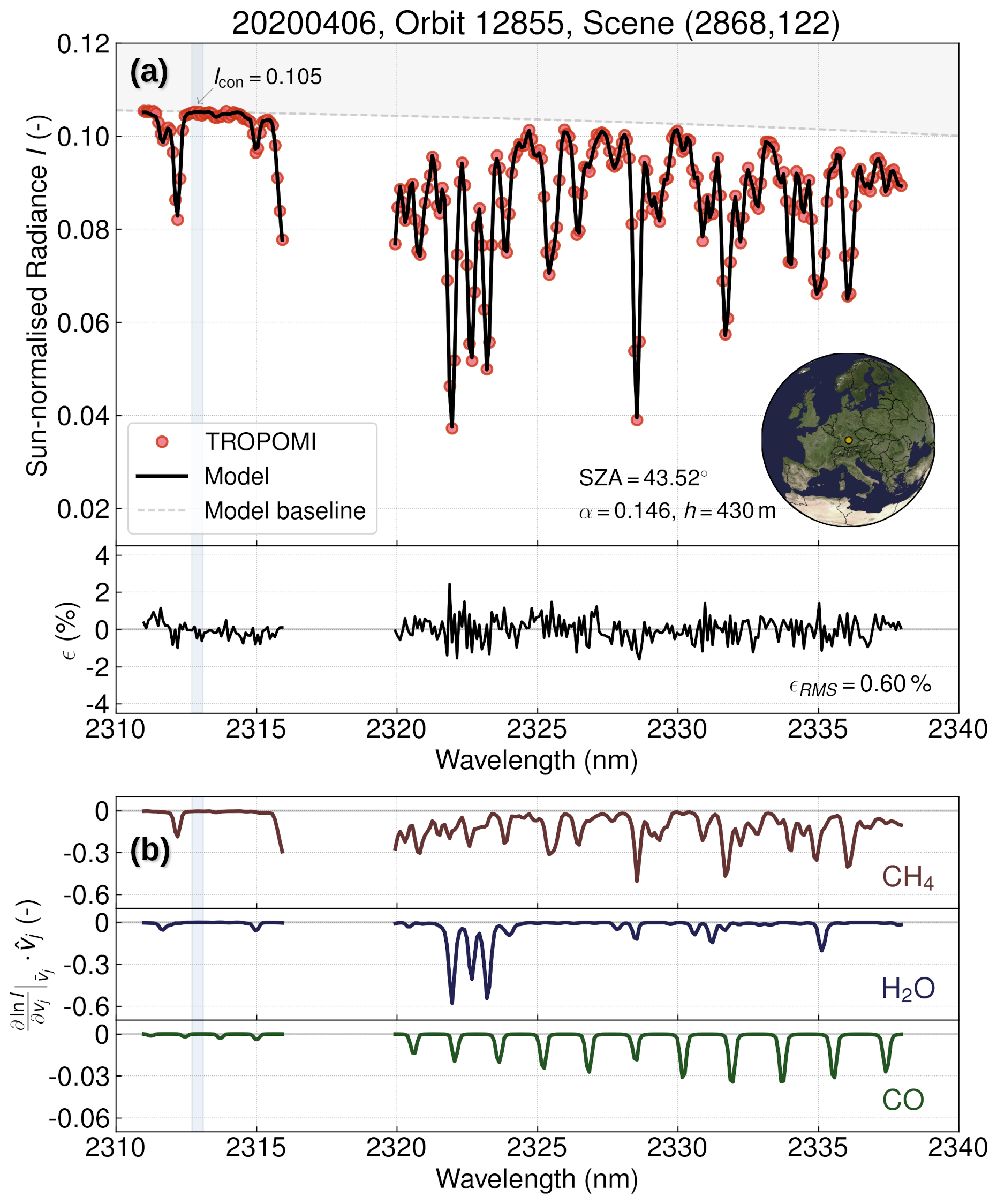
Figure A1 Spectral fit for a sample scene in Bavaria, Germany. (a) The TROPOMI spectral measurements (red circles) are shown together with the fitted radiative transfer model (black line) and the resulting (relative) fit residual ϵ below. The grey dashed line highlights the baseline of the model, i.e., the fitted polynomial without absorption. The difference between the baseline relative to the model or measurement gives a sense of the depth of the individual absorption lines. The blue-shaded interval indicates the virtually absorption-free continuum-like portion used to determine the apparent albedo, which is important to disentangle surface reflection and molecular abundances in the fitting procedure. (b) Weighting functions with respect to the fitted gases j scaled with the respective retrieved columns ${\widehat{v}}_j$, breaking down which of the measured features are attributable to which absorber. This representation also explicitly reconfirms that none of the gases has any significant absorption in the continuum-like interval used.

Appendix B: Perceptual uniform colormap vivian

It is increasingly recognised that scientific visualisation benefits from perceptually uniform colormaps, which enable accurate and accessible interpretation of data. Non-uniform changes in brightness or hue can distort the perception of quantitative values. Many conventional colour scales remain difficult to interpret, especially for viewers with colour vision deficiencies.

The vivian colormap, which is available in the Python package cmuseo, is designed to be perceptually uniform and accessible to people with colour vision deficiencies. Like the widely used viridis colormap, vivian targets the needs of scientific visualisation, but is intended to achieve a wider perceptual range. The perceptual gradient curve, used to assess the quality of colormaps, is generated by calculating the colour differences ΔE between adjacent colours using Euclidean distance in CAM02-UCS space, which closely models the human perception of colour. If the ΔE curve remains flat, this means that equal changes in the data translate into equal perceived differences, helping to preserve gradients and fine structures without introducing visual artefacts. We measure this flatness with the normalised root mean square (RMS) deviation ${\mathit{\delta }}_{\mathrm{RMS}}^{\mathit{\%}}$, which is reported as a percentage of the average ΔE. The total perceptual arc length $L={\int }_{\mathcal{C}}dE$ of the colormap's trajectory 𝒞 in the CAM02-UCS space reflects how large the perceptual range is that the colormap can cover, with larger L values indicating a better ability to reproduce fine details. In addition to ensuring the perceptual uniformity of the original colour information, it is also important that changes in brightness, calculated as $\mathrm{\Delta }{J}^{\prime }=\mathrm{\Delta }{E}_{(J^{\prime },\mathrm{0},\mathrm{0})}$, are likewise uniform and monotonic in order to guarantee flawless greyscale representation and better accessibility for viewers with limited colour perception.

Figure B1 shows that vivian is perfectly perceptually uniform, both in original colour representation and also when converted to greyscale, and is thus a reliable choice for accurate and accessible data visualisation in science. In line with the intended objective, the colormap offers a slightly larger perceptual range than viridis (L=145.0 versus 123.9).

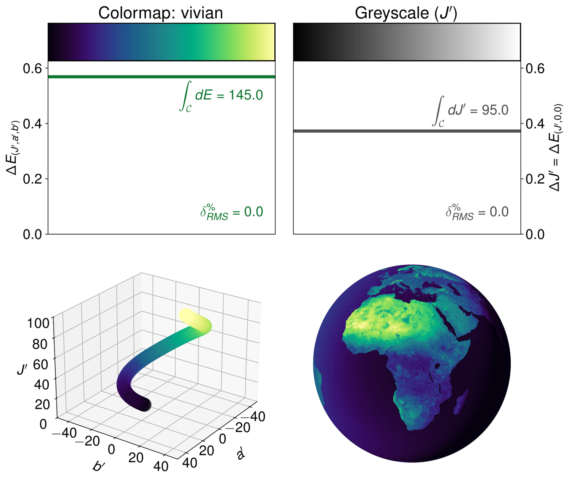
Figure B1 Perceptual analysis of the vivian colormap. Shown are perceptual differences along the colormap (top left) and corresponding lightness differences (top right) in CAM02-UCS space. The bottom panel shows the 3D-trajectory of vivian and an example figure.

Appendix C: List of TCCON sites

Strong et al. (2022)Batchelor et al. (2009)Buschmann et al. (2022)Kivi et al. (2022)Kivi and Heikkinen (2016)Wunch et al. (2022)Petri et al. (2024a)Messerschmidt et al. (2012)Notholt et al. (2022)Weidmann et al. (2023)Weidmann et al. (2025)Hase et al. (2024)Té et al. (2022)Warneke et al. (2024)Sussmann and Rettinger (2023)Wennberg et al. (2022b)Morino et al. (2022a)Zhou et al. (2022)Yang et al. (2020)Wennberg et al. (2022c)Morino et al. (2022b)Petri et al. (2024b)Iraci et al. (2022)Wennberg et al. (2022a)Shiomi et al. (2022)Ohyama et al. (2015)Liu et al. (2023)Wang et al. (2017)Morino et al. (2022c)Velazco et al. (2017)Deutscher et al. (2023b)Deutscher et al. (2010)De Mazière et al. (2022)Deutscher et al. (2023a)Sherlock et al. (2022)Pollard et al. (2022)Pollard et al. (2021)

Table C1 TCCON sites used in the validation sorted according to latitude from north to south.