Towards routine shipborne measurements of columnar CO₂, CH₄, CO, and NO₂: a case study for tracking regional-scaleemission patterns

Mobile remote sensing observations from shipborne platforms offer a unique opportunity for validating satellite observations and sampling plumes of greenhouse gases and short-lived air pollutants from the world’s highly populated coastal megacities and industrial sites. Here, we demonstrate the capabilities of a shipborne setup that combines a sun-viewing EM27/SUN Fourier transform spectrometer for the shortwave-infrared spectral range with a direct-sun DOAS (Differential Optical Absorption Spectroscopy) spectrometer for the visible spectral range, enabling simultaneous measurements of the column abundances of carbon dioxide (CO₂), methane (CH₄), carbon monoxide (CO), and nitrogen dioxide (NO₂). For several months in 2023 and 2024, the instruments were operating autonomously on a commercial vessel traveling back and forth along the coast of Japan. We show that, for CO₂, CH₄, and CO, precision and repeatability comply with the standards of the Collaborative Carbon Column Observing Network (COCCON). Further, for a case study in the vicinity of Nagoya, we demonstrate the scientific leverage of this mobile multi-species approach: Simultaneous measurement of CO₂, CO, and NO₂ enhancements is used to successfully disentangle emissions from different sources. Our study demonstrates that routine shipborne deployment is possible. The setup delivers highly precise and accurate trace gas abundance records of the target species and enables emission monitoring of sources due to their distinct emission ratios.

1 Introduction

The greenhouse gases carbon dioxide (CO₂) and methane (CH₄) drive climate change and thus are subject to manifold activities that aim at monitoring and verifying their emission rates, as required for the Paris Climate Agreement. Measuring CO₂ and CH₄ atmospheric abundances allows for independent verification of bottom-up statistical data and accounting reports when inverse transport modeling is used to derive top-down emission estimates from the observed concentration gradients (e.g., Reuter et al., 2014; Wong et al., 2015; Jones et al., 2021). In addition, column measurements of carbon monoxide (CO) and nitrogen dioxide (NO₂) can help attribute source type contributions for CO₂ since these air pollutants originate from combustion (together with CO₂) and the emission ratios between these three trace gases are specific to the processes and their efficiencies involved (Guevara et al., 2024). CO and NO₂, themselves, have adverse effects on human health, and thus, monitoring is warranted (Chen et al., 2007; Manisalidis et al., 2020).

Most commonly, atmospheric abundances of CO₂, CH₄, CO, and NO₂ can be measured through absorption spectroscopic techniques realized by in situ or remote sensing instruments. The latter have been deployed on satellites (e.g., Butz et al., 2011; Eldering et al., 2017; Van Geffen et al., 2022), on airborne platforms (e.g., O'Shea et al., 2014; Krautwurst et al., 2017; Leifer et al., 2018), or in ground-based networks (e.g., Dietrich et al., 2021; Luther et al., 2022; Herkommer et al., 2024). The Total Carbon Column Observing Network (TCCON; Wunch et al., 2011) and the COllaborative Carbon Column Observing Network (COCCON; Frey et al., 2019) host dozens of sun-viewing Fourier Transform Spectrometers (FTS) operating in the shortwave-infrared spectral range and providing the column-average dry-air mole fractions of CO₂ (XCO₂), CH₄ (XCH₄), and CO (XCO). The Pandonia Global Network (PGN; Herman et al., 2009) provides NO₂ columns among other air pollutants. Primarily, these networks have been designed for validating observations by satellites such as GOSAT (CO₂, CH₄; Butz et al., 2011), OCO-2 (CO₂; Eldering et al., 2017), GOSAT-2 (CO₂, CH₄, CO; Imasu et al., 2023), OCO-3 (CO₂; Taylor et al., 2020), Sentinel-5 Precursor (CH₄, CO, NO₂; Landgraf et al., 2016; Van Geffen et al., 2022), GOSAT-GW (CO₂, CH₄, NO₂; Tanimoto et al., 2025), and future missions such as CO₂M (CO₂, CH₄, NO₂; Sierk et al., 2021), and TANGO (CO₂, CH₄, NO₂; Brenny et al., 2023; Charuvil Asokan et al., 2025). Some of these missions use NO₂ not just as an informant for emission patterns but also, more technically, to geographically contour emission plumes from localized emitters such as coal-fired power plants and urban centers, thereby assisting in CO₂ emission estimates (Kuhlmann et al., 2021; Yang et al., 2023). In addition to providing essential validation for these satellite data, the ground-based measurements such as conducted within the TCCON and COCCON also give valuable constraints on local to regional emission patterns (Wunch et al., 2009; Babenhauserheide et al., 2020; Frey et al., 2021; Kiel et al., 2021; Ohyama et al., 2023).

Butz et al. (2022) reviewed the challenges and opportunities of implementing a mobile variant of the COCCON spectrometer (EM27/SUN Fourier transform spectrometer, Bruker Optics, Germany). Ship deployments of such spectrometers are appealing since they provide satellite validation over the oceans, which are currently only sparsely covered with validation data (Müller et al., 2021). If the ships commute along coastlines, shipborne observations can potentially constrain emission outflow from the upwind source regions. Here, we report on further development of our mobile COCCON spectrometer, whose ship deployment was showcased previously in Klappenbach et al. (2015), Knapp et al. (2021), and Butz et al. (2022), and which was used for land-based deployments to constrain localized emission patterns (Butz et al., 2017; Luther et al., 2019, 2022). This study introduces two key advances. First, we have successfully installed and remotely operated the mobile COCCON spectrometer on a commercial freighter that regularly sails Japan's coastline. Second, we co-mounted a DOAS unit measuring in the visible spectral range that allows for retrieving total column NO₂ alongside XCO₂, XCH₄, and XCO delivered by the EM27/SUN instrument. Thereby, simultaneously measuring several substances provides the opportunity to selectively attribute trace gas abundance variability to specific sources by examining vertical column densities (VCD) and emission ratios. A case study on Nagoya Bay demonstrates the system’s performance and shows how the combined trace-gas measurements enable source-selective emission verification.

2 Instrument setup

The instrument described in this work is an upgrade of a commercially available Bruker EM27/SUN Fourier-transform spectrometer (FTS) for the shortwave-infrared spectral range, recording the absorption features of CO₂, CH₄, CO, and O₂ (the latter for calculating mixing ratios) and a commercially available Ocean Optics QE-Pro spectrometer for the visible spectral range, resolving the individual absorption lines of NO₂, and potentially other trace gases in the future.

2.1 EM27/SUN FTS and solar tracker

The EM27/SUN FTS (Bruker Optics, Germany) is the standard instrument of the COCCON network for land-based observations of XCO₂, XCH₄, and XCO (Frey et al., 2019). Modifications and performance demonstrations for ship-based deployments are described in Klappenbach et al. (2015), Knapp et al. (2021), and Butz et al. (2022). Summarizing the most important features here, the EM27/SUN has an optical resolution of 0.5 cm⁻¹ and a semi-field-of-view of 2.36 mrad (Gisi et al., 2012; Frey et al., 2015). The latest EM27/SUN version contains two detectors. The first InGaAs photodetector covers the spectral range between 5500 and 11 000 cm⁻¹ (Gisi et al., 2012), where O₂, CO₂, and CH₄ absorption lines are present. The second InGaAs-detector with spectral extension towards the infrared covers the wavelength range between 4000 and 5500 cm⁻¹ (Hase et al., 2016), where CO absorption features can be found. The EM27/SUN FTS demonstrated its versatility and robustness under various climatic conditions and in different settings (Butz et al., 2017; Viatte et al., 2017; Luther et al., 2019; Humpage et al., 2021; Frey et al., 2021), making it an ideal instrument for campaign deployments. In addition, Frey et al. (2019) demonstrated its suitability in terms of stability and comparability for network applications such as those implemented through COCCON.

Our EM27/SUN is operated and characterized according to COCCON protocols, with two modifications. First, to avoid data loss in the case of tracker instability, we record individual interferograms for each forward-backward scan rather than relying on automatic co-adding of 10. Second, we use an interferogram sampling rate of 20 kHz (instead of 10 kHz). This leads to one forward-backward scan being completed approximately every 15 s. In addition to this, the solar tracker of the standard EM27/SUN is replaced by a custom-built system to be able to compensate for the rather quickly changing attitude and orientation of a ship platform. The high precision of our custom-built tracking system was demonstrated for shipborne deployments in Butz et al. (2022), and for balloonborne deployments in Voss et al. (2024), where more details on the tracking system can also be found. The instrument is housed in an aluminum box to protect it from harsh weather. The entire box is ventilated and equipped with various ancillary sensors for pressure and temperature measurements, and its position is tracked via GPS. Mats have been placed underneath the instrument to damp it from vibrations caused by the engine of the ship. Figure 1 shows the box with the instruments on board the commercial vessel Nichiyu Maru (Ocean Link, Ltd.) during the deployment described in Sect. 3.

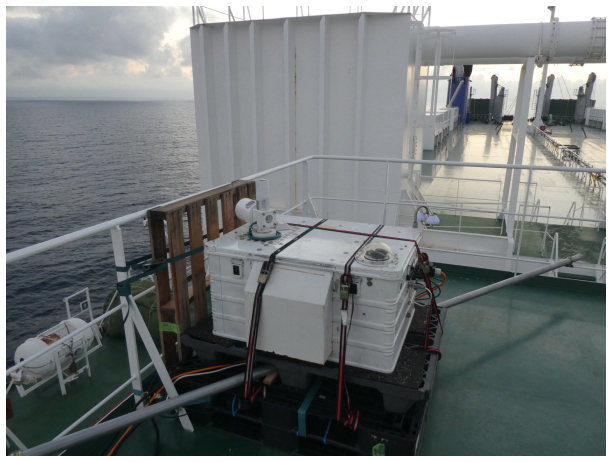
Figure 1 Box housing the EM27/SUN FTS, the DOAS spectrometer, and the sun tracker assembly. The box is positioned on the upper deck of the vehicle-carrier Nichiyu Maru (Ocean Link, Ltd.).

2.2 DOAS spectrometer

To supplement the setup with measurement capabilities for NO₂, we co-mounted a grating spectrometer measuring solar absorption spectra in the visible (VIS) spectral range. Using differential optical absorption spectroscopy (DOAS) (Platt and Stutz, 2008), NO₂ atmospheric column abundances are accessible. The DOAS instrument uses part of the light beam from the solar tracker, which is not needed for the FTS. This is possible since the beam from the solar tracker has a diameter approximately twice as large as the aperture of the FTS. The DOAS itself needs less than 0.15 % of the total beam diameter. The aperture of both instruments is sufficiently far away from the fringes of the beam of the tracker mirror. The part of the solar beam needed for the DOAS is coupled into an optical fiber (Laser Components FVP-400) using a custom-built telescope assembly similar to the one used in Butz et al. (2017) and Voss et al. (2024). The assembly consists of the following components, as schematically shown in Fig. 2: A prism (Thorlabs PS910) positioned under total-reflection relays the incoming beam into a lens tube with a bandpass filter centered at 460 nm (Edmund Optics Hoya B460). The field of view of the telescope is limited to 1.15° by focusing the light onto an 800 µm aperture (Edmund Optics 34-445) using a bi-convex lens (Thorlabs LB1027-A). Furthermore, the light is diffused before entering the fiber by a polytetrafluorethylene reflector plate mounted at a 45° angle with respect to the optical axis. The fiber is mounted so that only light from the reflector plate can enter it. The fiber is connected to an Ocean Optics QE-Pro spectrometer operating in a Czerny-Turner configuration (Czerny and Turner, 1930) in the visible spectral range.

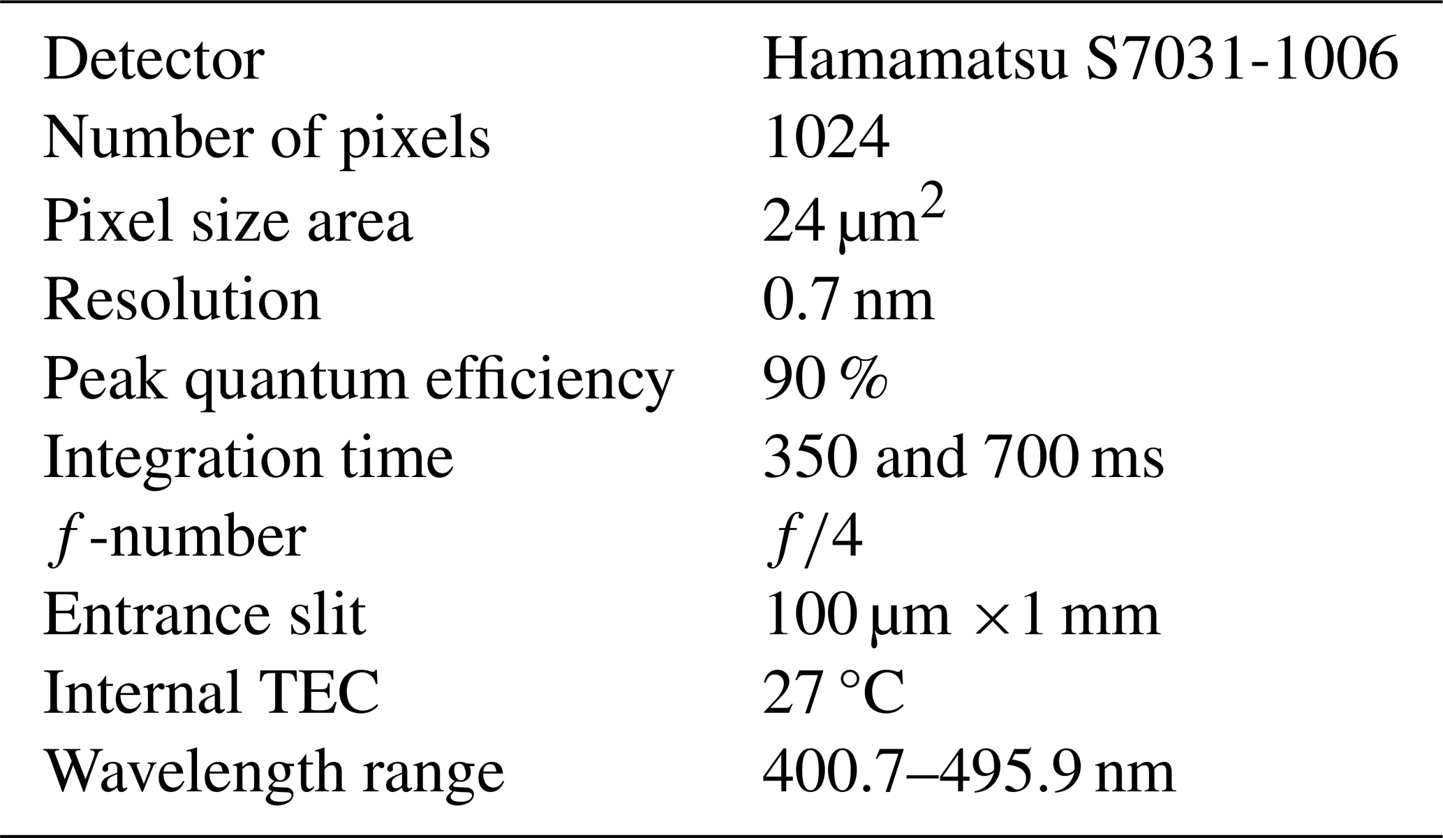
The technical data of the VIS spectrometer and the settings used during the deployment described in this work are listed in Table 1. The spectrometer entrance slit with a width of 100 µm defines the light throughput and the width of the spectral response function (SRF). The spectral sampling amounts to 5 detector pixels per full-width-at-half-maximum (FWHM) of the SRF, corresponding to 0.7 nm, as determined by measuring individual spectral emission lines from mercury and krypton emission lamps. The DOAS spectrometer is configured such that it records spectra in a wavelength range between 400.7 and 495.9 nm. Two different exposure times are used to maximize the signal but prevent saturation of the detector. At high solar zenith angles (SZA) during the morning and evening, spectra are recorded with an exposure time of 700 ms. At low SZA, the instrument is switched automatically to an exposure time of 350 ms.

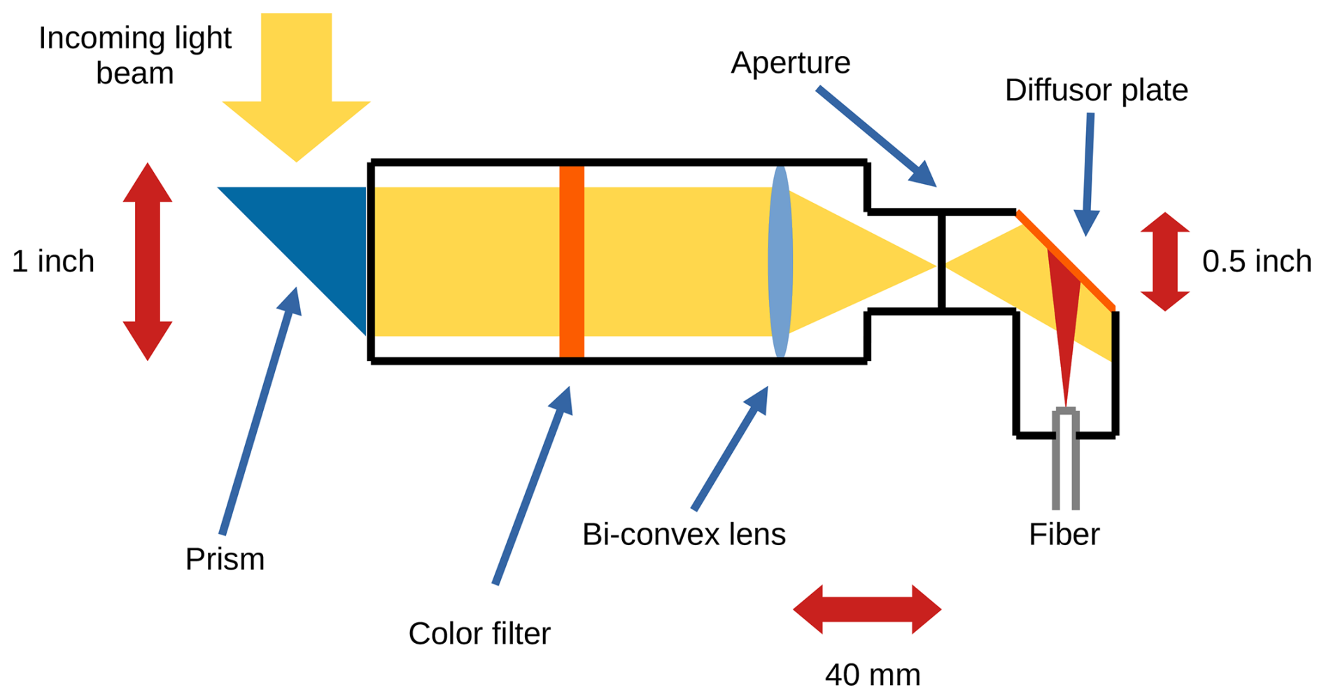
Figure 2 Schematics of the telescope of the DOAS instrument. The figure shows the telescope's components, including the prism, color filter, bi-convex lens, and aperture. The acceptance cone of the fiber, which is shown in red, indicates which part of the light beam is directed into the fiber. Drawing not to scale.

Table 1 Overview of the spectrometer specifications and the operational settings of the DOAS instrument during the deployment. Data partly taken from Ocean Optics, Inc. (2014).

A two-stage cooling is used to keep the DOAS spectrometer and its detector at constant temperatures. The first stage is the QE-Pro spectrometer's internal thermoelectric cooler (TEC). It can cool the detector down to 20 K below the ambient temperature. In addition, the spectrometer is housed inside a custom-built enclosure, which is sealed so that water vapor is prevented from entering by allowing exchange with the ambient air only through a silica gel tube. A second TEC is used to regulate the temperature inside this enclosure to an accuracy of ±0.1 K. This is, however, only possible for a temperature range of 2 K below and 15 K above the outside temperature. Since outside temperatures in the range between 0 and 40 °C occurred during the deployment, the external TEC was operated at temperatures between 10 and 38 °C, and the internal TEC at temperatures of up to 27 °C, which is not ideal in terms of noise reduction but ensures temperature stability throughout the deployment. An upgrade of the external TEC, facilitating stabilization at lower temperatures, is planned for the future. The current setup, however, already leads to a temperature stability of the DOAS detector better than ±0.0015 K on all days on which a proper temperature range with respect to the ambient conditions was selected.

For the campaign reported here, the SRF of the DOAS spectrometer was recorded by measuring the emission lines of krypton or mercury lamps. We conducted these lamp measurements before and after the campaign deployment and approximately every six weeks while the instrument was onboard the ship. All SRFs show shape deviations of less than 4 % relative to the peak height of the first SRF measurement. In addition, it was verified by re-running the analysis (see Sect. 4.2) with several different SRFs measured throughout the campaign that changing the SRF used in the retrieval leads to changes of the result for the vertical column density (VCD) of NO₂ of up to 0.75 %, which is much smaller than the overall retrieval error between 2 % and 14 % (depending on weather conditions). This leads to the conclusion that the grating spectrometer remained stable throughout the deployment. Since the remarkable ensemble performance of DOAS instruments was already demonstrated, e.g., in Piters et al. (2012), and the stability and high accuracy of QE Pro spectrometers were demonstrated during long-term ground-based (Grossmann et al., 2018) deployments, as well as during aircraft-based (Stutz et al., 2017) and balloonborne measurements (Voss et al., 2024), additional performance tests, as done for the FTS (see Sect. 4.3), are not needed for this instrument.

2.3 Remote access

During previous campaigns, the instrument required an operator onboard the vessel (e.g., Butz et al., 2022). For the present campaign, the instrument was upgraded to operate fully automatically and to allow for remote access. To this end, custom-built software packages were used to automatically operate the two spectrometers, the temperature stabilization, all ancillary sensors, and the solar tracker. A maintenance crew only needed to go on board the vessel approximately every six weeks to exchange the hard drives used to store the data and to perform characterization measurements. In order to allow for remote access for quick instrument checks and to notify the maintenance crew in case of instrument errors, access via the mobile phone network using an MC Technologies MC100 network switch with a Quectel EG21-1 module was installed. A 1.5 m long 790–960 MHz multiband antenna from MC Technologies with 6 dBi antenna gain was mounted on the ship's railing. Since the ship was traveling along the coast of Japan (see Sect. 3), this antenna was large enough to connect to the instrument on about 80 % of the route.

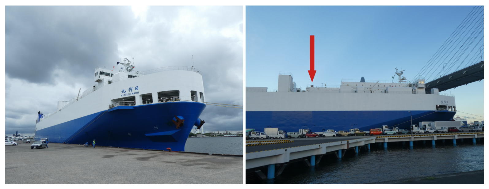
Figure 3 The vehicle carrier Nichiyu Maru (Ocean Link, Ltd.) (left) and the location of the instrument on the ship (right). The instrument is marked with a red arrow.

3 Campaign overview

The vehicle carrier Nichiyu Maru offered the opportunity to test our setup with rather short lead times within the framework of the Ship of Opportunity (SOOP; https://www.soop.jp/, last access: 15 September 2025) program by the National Institute for Environmental Studies (NIES). The ship travels along the coast of Japan, having a weekly round-trip schedule. This makes it possible to probe the emissions of major industrial areas of Japan up to twice per week, depending on weather conditions. The Nichiyu Maru is therefore an ideal platform to test the use of our instrument for emission monitoring. In addition, the route of the Nichiyu Maru allows for easy access since remote monitoring via the mobile phone network is possible (see Sect. 2.3) and maintenance access in a harbor close to NIES is possible once per week if needed. Finally, meteorological and chemical in situ data from the other instruments on board the Nichiyu Maru within the framework of SOOP is available, paving the way for future multi-instrument studies.

The Nichiyu Maru (Fig. 3), owned by Ocean Link, Ltd., is 160 m long, 25 m wide, and was built in 2019 (Nippon Kaiji Kyokai, 2024). Our instrumentation was installed on board the Nichiyu Maru (Fig. 1) from 16 September to 16 December 2023 and from 17 February to 22 May 2024. Between the two periods, the ship was in the dry dock for maintenance. The instruments were positioned on the ship's upper deck at the location behind the bridge marked with the red arrow in Fig. 3. Care was taken to choose a location far away and in front of the chimney to prevent the ship's exhaust plume from interfering with the measurements. Indeed, no plume signatures were found in the spectra recorded while the ship was moving. The instrument's location corresponds to an average altitude between 27 and 30 m above sea level (as measured by the GPS sensor of the instrument), depending on how heavily the Nichiyu Maru was loaded.

During the deployment described here, the Nichiyu Maru traveled along the east coast of Japan from the port of Kawasaki (Bay of Tokyo) to the port of Kanda (Fukuoka prefecture) and back once per week. It usually stopped at the ports of Nagoya, Sakaide (Takamatsu prefecture), Kurashiki (Okayama prefecture), and Hiroshima on the way from Kawasaki to Kanda, and at the ports of Kurashiki (Okayama prefecture), Toyohashi (Aichi prefecture), and Yokosuka (Bay of Tokyo) on the way back to Kawasaki. Additional stops occurred during some round trips in spring 2024, e.g., in Kobe (Hyogo prefecture). Although the Nichiyu Maru often is moored in the harbors during the day to load and unload vehicles and mostly sails at night, we were able to collect daytime measurements in the Seto Sea between Kitakyushu and Osaka, in the Nagoya region, and in the Bay of Tokyo (see Fig. 4) that allow for technical testing and for showcasing source attribution. In total, daytime measurements are available for 112 d of the deployment. On 57 of these days, the weather conditions were favorable enough to have useful data produced at least during part of the day (see Sect. 4 for information on quality filters included in the retrieval).

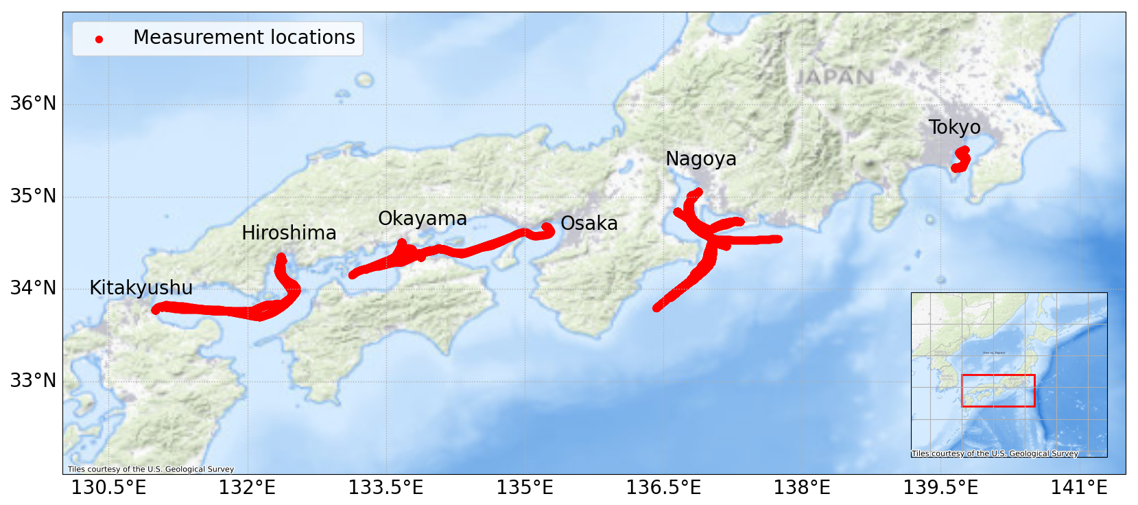
Figure 4 Locations (red) of the columnar measurements collected onboard the vessel Nichiyu Maru between September 2023 and May 2024. Basemap courtesy of the US Geological Survey.

4 Retrieval and data quality assurance

The retrieval procedure for CO₂, CH₄, and CO from EM27/SUN observations is described in Sect. 4.1 mostly following previous work (Klappenbach et al., 2015; Knapp et al., 2021; Butz et al., 2022). The retrieval of NO₂ from observations of the DOAS instrument is described in Sect. 4.2 following the DOAS principles (Platt and Stutz, 2008).

4.1 Retrieval of CO₂, CH₄, and CO from EM27/SUN measurements

In a first step, the interferograms recorded by the EM27/SUN FTS need to be Fourier transformed into spectra. To this end, as in our previous work, the preprocessor of the PROFFAST retrieval software (Hase, 2000; Frey et al., 2021) is used, which is also employed for EM27/SUN data processing within the COCCON network (Frey et al., 2019). We use a spectral window of 3500 to 14 000 cm⁻¹ for channel 1 and 3000 to 5200 cm⁻¹ for channel 2 of the FTS, a Mertz (1967) phase correction, and a Norton-Beer medium apodization (Norton and Beer, 1976, 1977) throughout this study. Before the Fourier transform, the direct current (DC) component of the interferograms is used to filter out scenes with low brightness or large brightness fluctuations following Klappenbach et al. (2015) and Butz et al. (2022). Large brightness fluctuations indicate clouds passing by or the tracker not fully compensating for the ship's motion. Following Knapp et al. (2021), the DC-variability of an interferogram can be defined as

$$\begin{array}{}\text{(1)}& {\text{DC}}_{\text{var}}={\displaystyle \frac{\text{max}\left(I_{\text{DC}}\right)}{\text{min}\left(I_{\text{DC}}\right)}}-\mathrm{1}\end{array}$$

where I_DC is the intensity of the DC-component of the interferogram. All interferograms with a DC-variability greater than 5 % throughout the integration time of the measurement are filtered out. In addition, a low average DC value can indicate clouds passing in front of the sun. Therefore, interferograms with an average DC value lower than 5 % are excluded from any further analysis.

The algorithm RemoTeC (Butz et al., 2011) performs the actual spectral retrieval. It was chosen here since the standard algorithm of the COCCON network, PROFFAST, currently does not yet accept moving instruments. The RemoTeC algorithm was originally developed for the retrieval of gas abundances from the GOSAT satellite (Butz et al., 2011) but has since been applied to various satellites, including OCO-2 (Wu et al., 2018) and TROPOMI (Hu et al., 2016). Adapted versions for ground-based applications exist and have been applied to a variety of settings (e.g., Klappenbach et al., 2015; Luther et al., 2019; Knapp et al., 2021; Löw et al., 2023). For ground-based direct sun applications, RemoTeC neglects scattering, reducing the radiative transfer equation to Beer-Lambert's law. A priori profiles for the retrieval are calculated based on meteorological data from NCEP (National Centers for Environmental Prediction et al., 2000), in situ ground-based pressure and temperature measurements, standard profiles for CH₄ and CO₂ from tracer model 4 (TM4) (Dentener et al., 2003; Meirink et al., 2006) and CarbonTracker (Peters et al., 2007) as well as standard profiles for CO based on tracer model 5 (TM5) (Huijnen et al., 2010). Spectral line parameters are taken from HITRAN 2016 (Gordon et al., 2017). The solar top-of-the-atmosphere reference spectrum is provided by Geoffrey Toon (2016, personal communication).

Formally, RemoTeC retrieves partial column densities for six altitude layers, which are equidistant in pressure, employing a Phillips-Tikhonov regularization scheme (Phillips, 1962; Tikhonov, 1963). Each target species' vertical column density (VCD) is then calculated by summing up the partial columns in these six layers. The forward model itself is calculated for 72 atmospheric layers based on Voigt line shapes. The forward model convolves the line-by-line spectra by the instrument SRF (often also called instrument lineshape (ILS) in the context of FTS) to simulate the observed spectra. The SRF was recorded on 23 August 2023, following the procedures of the COCCON protocol (Frey et al., 2015, 2019). Table 2 lists the spectral windows used for the retrieval of CO₂, CH₄, and CO as well as for molecular oxygen O₂. Water vapor H₂O is an interfering absorber.

Table 2 Spectral windows and respective absorbing gases for the EM27/SUN measurements.

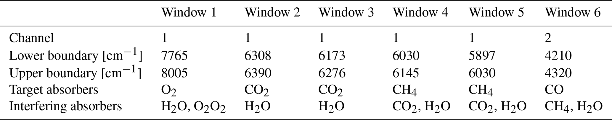
We use the retrieved O₂ and H₂O column densities to calculate the total pressure at the instrument level and call it “spectroscopic” pressure p_spec since it is derived from spectroscopic measurements. For quality assurance, the spectroscopic pressure can be compared to the in situ surface pressure p_in-situ measured by a co-deployed pressure sensor (cf. also Knapp et al., 2021). Deviations (on top of trivial offset factors between spectroscopic and in situ data) indicate potential error sources of our setup, such as pointing errors of the solar tracker, drifts of the optical alignment, or spectroscopic parameter errors. Therefore, we use spectroscopic pressure as a quality filter as follows:

1. We remove outliers with $\left|\mathrm{1}-\frac{p_{\text{spec}}}{p_{\text{in-situ}}}\right|<\mathrm{0.05}$.

2. Be R the average ratio $\frac{p_{\text{spec}}}{p_{\text{in-situ}}}$ over the entire campaign. We remove all data with $\left|\mathrm{1}-\frac{p_{\text{spec}}}{p_{\text{in-situ}}\times R}\right|<\mathrm{0.003}$.

Further details on this filtering approach can be found in Klappenbach et al. (2015) and Knapp et al. (2021).

After filtering, the remaining VCDs of the absorbers are generated by averaging over ten consecutive retrievals to improve the signal-to-noise ratio and to make the dataset comparable to the COCCON standard (Frey et al., 2019). Averaging is stopped at a smaller number if gaps are detected. The column-average dry-air mole fractions X_GAS for a specific gas, from now on called mixing ratio, are calculated through

$$\begin{array}{}\text{(2)}& X_{\text{GAS}}={\displaystyle \frac{{\text{VCD}}_{\text{GAS}}}{{\text{VCD}}_{{\mathrm{O}}_{\mathrm{2}}}}}\times \mathrm{0.2095}\end{array}$$

(Wunch et al., 2011). Based on the side-by-side measurements described in Sect. 4.3, the VCDs and X_GAS are multiplied by a scaling factor such that they correspond to the ones measured by the TCCON station in Tsukuba. Finally, as recommended by Wunch et al. (2011), an empirical correction for a spurious airmass-dependent bias is applied as follows:

$$\begin{array}{}\text{(3)}& Z_{\text{GAS,corr}}\left(\mathrm{\Theta }\right)={\displaystyle \frac{Z_{\text{GAS}}\left(\mathrm{\Theta }\right)}{a{\mathrm{\Theta }}^{\mathrm{3}}+b\mathrm{\Theta }+c}}\end{array}$$

where Z is either a mixing ratio or a VCD, Θ is the SZA, and a, b, and c are empirically determined coefficients. These coefficients are based on measurements from Knapp et al. (2021), who previously used the same instrument for background measurements over the Pacific Ocean. It should be pointed out that this correction is applied to mixing ratios and VCDs separately, since the VCDs are later used to calculate enhancement ratios with respect to NO₂ VCDs, and the airmass-dependent bias is different in the O₂ and in the target gas retrieval windows.

4.2 Retrieval of NO₂ from DOAS measurements

Since, in contrast to CO₂ or CH₄ absorption in the near-infrared, absorption optical thicknesses of NO₂ are typically minor in the visible spectral range, we can apply the DOAS technique (Platt and Stutz, 2008) to infer NO₂ column densities from the measurements of the VIS spectrometer. The DOAS retrieval consists of several steps. A dark current, offset, and non-linearity correction is performed during preprocessing. Dark current and offset spectra are measured every night at 02:00 a.m. local time throughout the campaign and are then used for the respective correction. A non-linearity correction is performed using a ninth-degree polynomial, which was determined in the laboratory based on measurements of a halogen light source recorded at various exposures. Afterwards, typically 100 spectra (corresponding to between 30 and 90 s of measurements, depending on the exposure time) are co-added. The co-addition is stopped at less than 100 spectra if the exposure time changes, the spectra have a saturation of less than 8 % (which is typical for measurements during sunrise and sunset or during the presence of larger clouds), large saturation fluctuations are detected (which relates to perturbed sun-tracking), the time between two subsequent spectra is longer than 70 s, or spectra are missing between subsequent measurements. All co-added spectra consisting of fewer than 50 measurements are discarded.

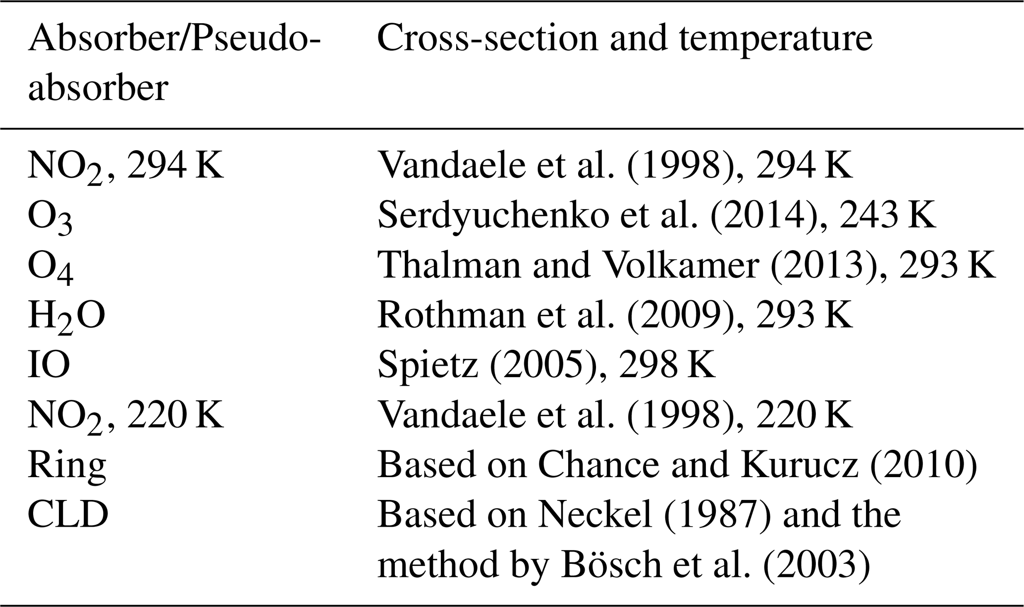
After the preprocessing, the DOAS fit is performed using the software package QDOAS (Danckaert et al., 2017). QDOAS recalibrates the initial pixel-to-wavelength mapping based on the solar Fraunhofer lines as a first step. Then, the actual DOAS fit, based on Beer-Lambert's law, finds the differential slant column densities (dSCDs) of NO₂ and interfering absorbing gases together with ancillary parameters such as spectral shifts, a background polynomial, an intensity offset parameter accounting for instrument straylight, as well as a center-to-limb-darkening (CLD) and Ring effect correction required for direct-sun measurements in the presence of scattering due to high-altitude clouds. The latter is a typical weather condition during the deployment of the instrument. All DOAS fit parameters are detailed in Table 3, and a list of all absorption cross-sections used can be found in Table 4.

Chance and Kurucz (2010)

Table 3 Parameters of the DOAS fit.

Vandaele et al. (1998)Serdyuchenko et al. (2014)Thalman and Volkamer (2013)Rothman et al. (2009)Spietz (2005)Vandaele et al. (1998)Chance and Kurucz (2010)Neckel (1987)Bösch et al. (2003)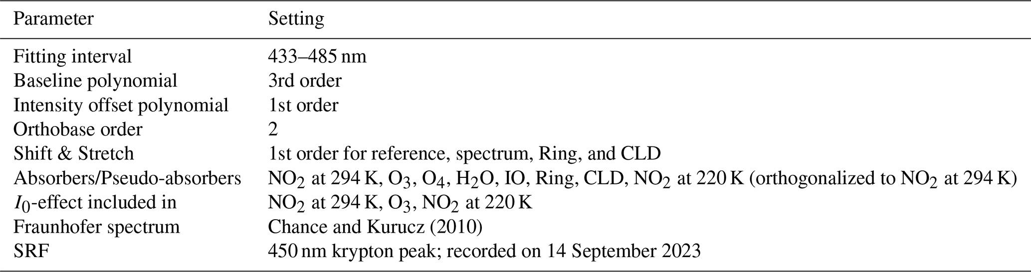

Table 4 List of absorption cross-sections and pseudo-cross-sections used in the DOAS retrieval.

One of the key aspects of DOAS is that the retrieval finds dSCDs with respect to a reference spectrum I₀ measured by the very same spectrometer. In our case, this reference spectrum, taken for the entire campaign dataset, is recorded around noon under minimal airmass and cloud-free conditions on 17 October 2023. To get the total slant column densities (SCDs) throughout the atmosphere, we need to add the absorber slant column density contained in the reference spectrum SCD_ref to the dSCDs found by the DOAS fit. To find SCD_ref, we use an approach similar to the procedures of the PANDONIA network (Herman et al., 2009) and the bootstrap method by Cede et al. (2006). The approach builds on Langley's method (Langley, 1904), which assumes the following linear relation for absorber i

$$\begin{array}{}\text{(4)}& {\text{dSCD}}_i={\text{VCD}}_i\times {\text{AMF}}_i\mathrm{-}{\text{SCD}}_{\text{ref}}\end{array}$$

where AMF_i is the air-mass factor, which can be approximated as $\text{AMF}=\frac{\mathrm{1}}{\text{cos}\mathrm{\Theta }}$ as long as SZA Θ<70° (Platt and Stutz, 2008). Thus, SCD_ref is the ordinate intercept of a plot of the dSCDs versus the AMF.

Langley's method is only applicable for background measurements where the gas concentrations do not change over the range of SZA used for the plot, i.e., over the course of a day. Since our NO₂ measurements are conducted in the vicinity of local NO₂ sources and NO₂ is variable due to photochemistry and meteorological transport, our measurements do not fully comply with this assumption. However, since we use a single reference spectrum for the entire campaign period, we can assemble a composite Langley plot for NO₂ spanning many days as shown in Fig. 5. The composite Langley plot reveals a sharp, well-defined lower boundary, defined by background conditions composed of many individual days. To find SCD_ref, we define background conditions as the 20 % lowest dSCDs in each 0.1 AMF bin (orange data in Fig. 5) and fit the linear relationship given by Eq. (4) to this background data. For uncertainty estimation, we use a bootstrap method, repeating the fit procedure multiple times with randomly chosen subsets of the background data and taking the maximum and minimum of the found SCD_ref as the error range. The error introduced by arbitrarily choosing 20 % as a threshold was estimated by re-running the whole analysis with different thresholds between 5 % and 40 %. The total error is then the Gaussian sum of the error of the bootstrap realizations (0.51×10¹⁵ molec. cm⁻²) and the error determined by changing the threshold (0.68×10¹⁵ molec. cm⁻²). Based on this method, we find SCD${}_{\text{ref}}=(-\mathrm{7.02}\pm \mathrm{0.85})\times {\mathrm{10}}^{\mathrm{15}}$ molec. cm⁻² for NO₂, which is used to calculate total SCDs and together with the AMF the respective VCDs of NO₂.

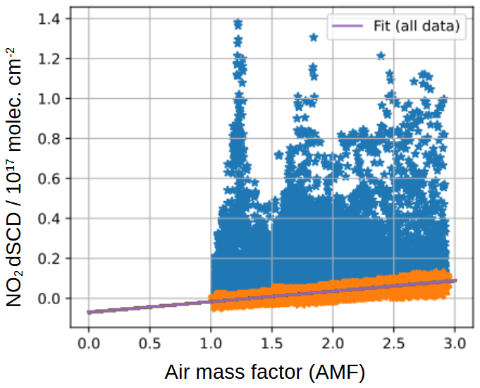
Figure 5 NO₂ Langley plot for the entire campaign dataset. Orange dots indicate background conditions used for finding SCD_ref. The purple line is the linear fit to all background data. The width of the purple line represents the ensemble of all bootstrap realizations used to calculate the error of SCD_ref.

Finally, quality filtering is applied to the NO₂ VCDs. Measurements with SZA >70° are filtered out since the cosine approximation used to calculate the AMF is not valid due to Earth's curvature becoming non-negligible (Platt and Stutz, 2008). Also, all measurements with a root-mean-square spectral fitting error (RMSE) of more than five times the average RMSE of the respective measurement day are discarded since a large RMSE indicates brightness fluctuations during the measurement, e.g., caused by variable cloud cover disturbing the solar tracking. Finally, for calculating ratios with respect to gases measured by the EM27/SUN, the NO₂ VCDs are also downsampled to the frequency of the EM27/SUN measurements by averaging the DOAS measurements to the time intervals of the EM27/SUN dataset. This averaging results in one datapoint every 2.5 to 3 min.

4.3 Performance of the EM27/SUN spectrometer and comparison to instruments of the COCCON network

Shipborne deployments are a major challenge for FTS. Especially shocks during the transport of the instrument to the ship or constant vibrations on board, e.g., caused by the engine of the ship, may lead to misalignments or instrumental drift. For future operation of our instrument, for example, within the COCCON, it is crucial to verify that it remains stable throughout the deployment and can be operated within the error margin of land-based spectrometers. The important criteria for benchmarking the stability of an EM27/SUN FTS are the change of the spectral response function (SRF, often also referred to as instrument line shape (ILS)) and the drift of the spectrometer with respect to an instrument of a high-resolution, ground-based FTS network such as the Total Column Carbon Observing Network (TCCON). These two criteria were monitored throughout the deployment and are discussed in the following. For additional performance tests, including an evaluation of the precision of the tracking system while the ship was in motion, the reader is referred to Knapp et al. (2021) and Butz et al. (2022).

SRF measurements with the FTS were conducted before and after the deployment, as well as during the ship's maintenance break. These measurements were conducted following the procedure described in Frey et al. (2015) under controlled laboratory conditions. SRF measurements are impossible on the ship itself since the lamp assembly cannot be reliably set up onboard. All SRF measurements are evaluated with the retrieval software LINEFIT 14.6 (Hase, 2000) as described in Frey et al. (2015) and Frey et al. (2019) to be consistent with SRF measurements from previous campaigns.

Panels a and c of Fig. 6 show the modulation efficiency (ME) and the phase error (PE), respectively, of all SRF measurements conducted during the current deployment with the FTS. Since the instrument was not re-aligned since 2019, previous SRF measurements already reported in Knapp et al. (2021) and Hanft (2021), as well as previously unpublished SRF results from a deployment in 2022, are included in the figure. It should be noted that an abrupt SRF change reported in Knapp et al. (2021), which was at that time attributed to a shock during the transport from Heidelberg to Vancouver, was, in the meantime, attributed to a malfunction of the ancillary humidity sensor. After correction of this malfunction, the previously reported change disappears, as can be seen in Fig. 6.

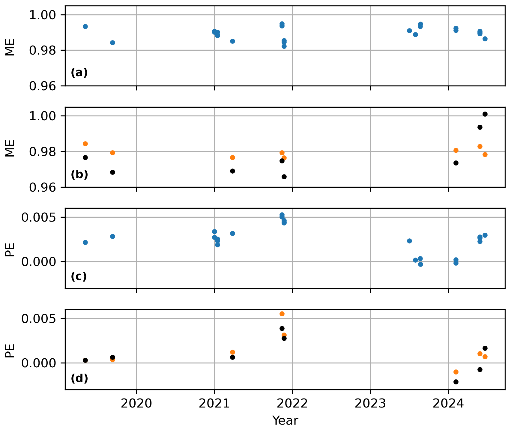
Figure 6 Overview of all spectral response function (SRF) measurements for the FTS conducted under controlled conditions in the laboratory since 2019. (a) and (c) show the modulation efficiency (ME) and the phase error (PE), respectively, for an SRF retrieved based on the water vapor absorption lines in the spectral region between 7000 and 7400 cm⁻¹ as used in the standard retrieval procedure described in Frey et al. (2015). (b) and (d) show ME and PE retrieved based on the water vapor absorption in the overlap region between the two detectors (5275–5400 cm⁻¹) as recommended by Alberti et al. (2022). Orange dots are results from detector channel 1 (used to retrieve CO₂ and CH₄). Black dots are results from detector channel 2 (used to retrieve CO).

During the current, latest deployment, our instrument has a ME of 0.9908±0.0023 and a PE of 0.0013±0.0013. If the whole data since 2019 is considered, our instrument has a ME of 0.9895±0.0034 and a PE of 0.0025±0.0016. These numbers for ME and PE and the respective errors are similar to those reported by Herkommer et al. (2024) for the COCCON travel standard (ME: 0.9805±0.0027, PE: $-\mathrm{0.0020}\pm \mathrm{0.0006}$) and the reference instrument SN-37 of the COCCON network (ME: 0.9836±0.0027, PE: 0.0015±0.0012). Our results for ME and PE are also within the range known from other COCCON instruments as reported by Alberti et al. (2022), and our standard deviation for ME for the current campaign is smaller than the error budget of 0.29 % derived by Frey et al. (2019) for the SRF retrieval procedure used in our study. Based on this, we conclude that despite frequent transports by aircraft and potential rough handling during craning, the SRF of our instrument has remained stable, and its changes are within the error margin of other instruments in the COCCON network. Thus, the same SRF measurement is used to evaluate the whole deployment (see Sect. 4.1).

As recommended by Alberti et al. (2022), the SRF of the second channel used for the retrieval of CO is also evaluated and compared to a SRF retrieval from the main detector channel based on water vapor absorption in the 5275 to 5400 cm⁻¹ spectral window, where both detectors are sensitive. The results are shown in panels b and d of Fig. 6. The deviations between the ME and the PE of the two channels of our EM27/SUN are similar to those reported by Alberti et al. (2022) for other instruments of the COCCON network. In addition, changes between the different measurements are similar to those for the standard SRF retrieval shown in panels a and c of Fig. 6. Only in May 2024, the ME of channel 2 (black dots in Fig. 6) is found somewhat higher than before and is also higher than the ME for detector channel 1. It is assumed that this change is caused by an incident where the crane bumped the spectrometer against parts of the ship when it was lifted to the upper deck in February 2024, leading to a slight misalignment of the second detector channel. Since we consider the SRF measurement based on channel 1 more reliable, we have used an SRF from that channel for the final retrieval described in Sect. 4.1.

In addition to monitoring the SRF, our instrument has been regularly compared to an instrument of the COCCON network (SN-147). Roughly every six weeks, we operated the two instruments side-by-side in the harbor of Kawasaki (Tokyo metropolitan area). For this, both EM27/SUN instruments were placed on the deck of the vessel Nichiyu Maru. Additional comparison measurements in the courtyard of NIES in Tsukuba were performed before and after the campaign, as well as during a maintenance break in February 2024. The COCCON instrument itself is regularly compared to the TCCON station in Tsukuba (Ohyama et al., 2009) to ensure a good quality of the COCCON instrument.

To evaluate the stability of our EM27/SUN with respect to the COCCON instrument, average ratios between the two instruments are calculated for the VCDs and X_GAS for all individual days when side-by-side measurements were conducted. The data reduction for measurements of the shipborne EM27/SUN follows Sect. 4.1. The measurements of the COCCON instrument are processed according to the standard COCCON protocol (Frey et al., 2019), relying on the retrieval software PROFFAST.

Table 5 Scaling factors of X_GAS and VCDs measured by the shipborne EM27/SUN and the COCCON instrument (SN-147) during side-by-side measurements. The table lists the daily average ratios calculated as the COCCON data divided by the data from the shipborne instrument. Side-by-side measurements took place in Kawasaki harbor and at NIES in Tsukuba.

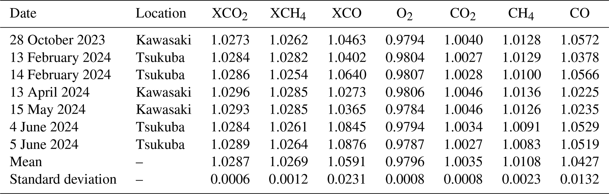
Table 5 lists the daily ratios between the gas retrievals from the COCCON measurements and those of the shipborne EM27/SUN. Based on the seven comparison days, average ratios of 1.0287±0.0006 for XCO₂, of 1.0269±0.0012 for XCH₄, and of 1.0591±0.0231 for XCO are found. The overall ratios are larger than the ones between different COCCON instruments reported by Alberti et al. (2022), which is related to differences in RemoTeC and PROFFAST. Most importantly, PROFFAST corrects for a spectroscopic error in the O₂-column, which accounts for a bias of about 2 % (Wunch et al., 2010), and already has an overall scaling factor with respect to the standards of the World Meteorological Organization (WMO) included, while RemoTeC leaves these corrections to the post-processing. In addition, our RemoTeC retrieval uses a different spectroscopic database (see Sect. 4.1) than PROFFAST, which leads to well-known offsets (Malina et al., 2022; Sha et al., 2020). A correction for the difference between RemoTeC and PROFFAST is later applied through an overall scaling factor with respect to TCCON in the retrieval as described in Sect. 4.1.

Inter-day differences are small for XCO₂ and XCH₄ as well as for the VCDs of O₂, CO₂, and CH₄, as can be inferred from the standard deviations listed in Table 5. Inter-day differences are larger for XCO and the VCDs of CO, but the overall accuracy and precision requirement is much less stringent than for CO₂ and CH₄. For CO, intra-day differences show an SZA dependency on the same order of magnitude as the inter-day variability.

Our standard deviations for XCO₂ and XCH₄ listed in Table 5 have a similar order of magnitude as the ones reported by Frey et al. (2019) for the reference instrument of COCCON with respect to TCCON (0.0015 for XCO₂, 0.0024 for XCH₄), which are, however, based on data from a much longer time series. Thus, our assessment suggests that our shipborne EM27/SUN complies with the standards of the COCCON network. The overall scaling factors for our instrument with respect to TCCON were calculated by multiplying our scaling factors from the comparison measurement in Kawasaki on 28 October 2023 with average scaling factors from comparison measurements between the COCCON instrument and the TCCON station in Tsukuba made in 2023 (see Table 6). The TCCON data is retrieved with the standard GGG2020 algorithm (Laughner et al., 2024).

Table 6 Overall scaling factors applied to X_GAS and VCDs retrieved from the shipborne EM27/SUN measurements to make them consistent with the TCCON measurements in Tsukuba.

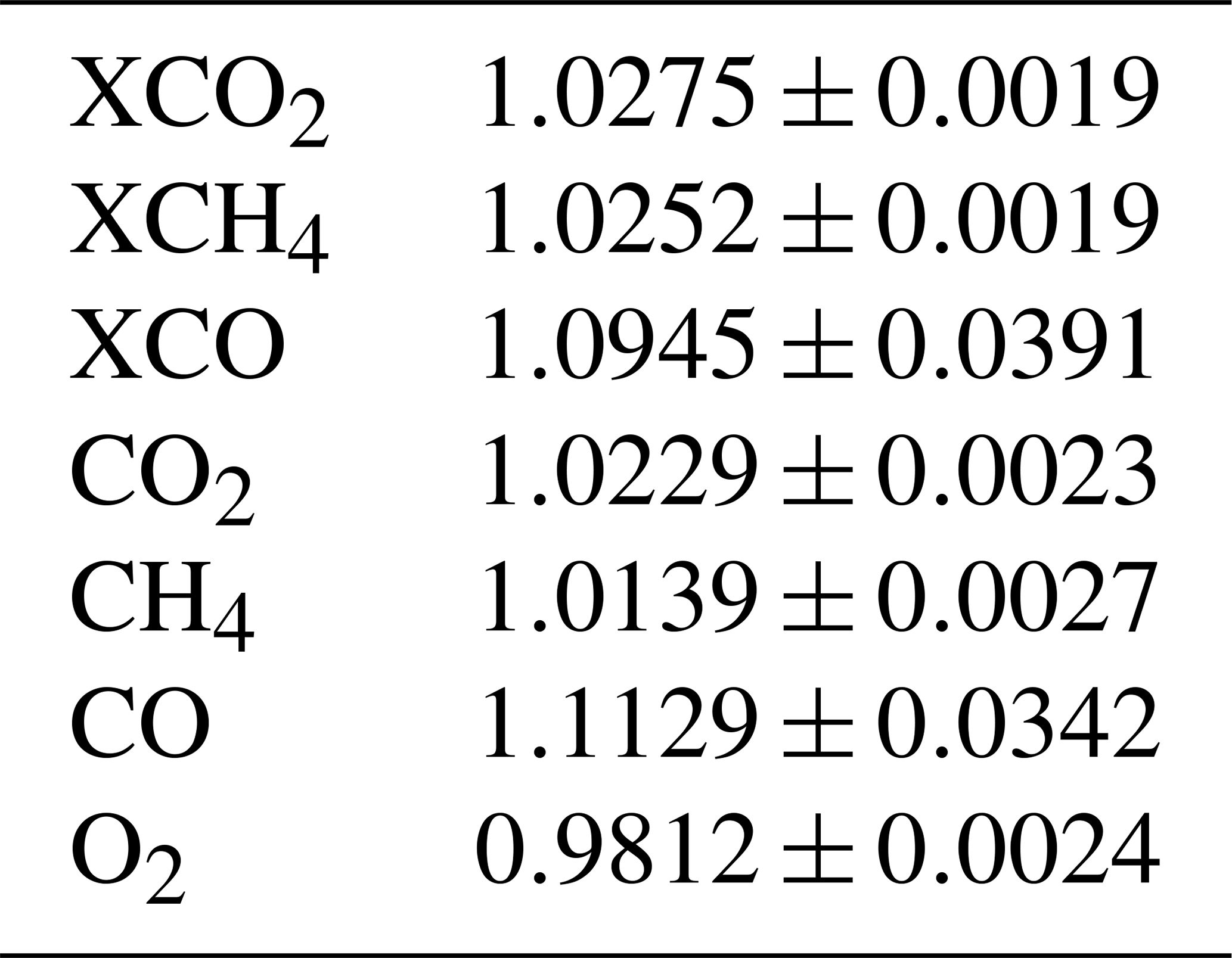
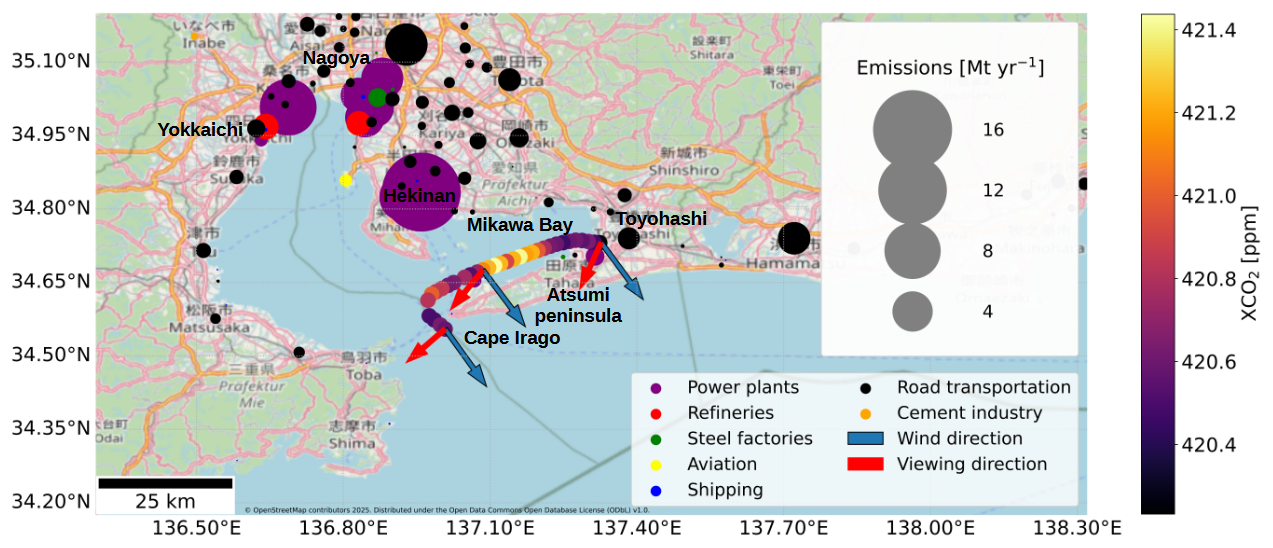
Figure 7 Overview of the case study in Mikawa Bay on 13 November 2023. The ship's trajectory from Toyohashi to Cape Irago is illustrated through color coding of the XCO₂ measurements collected by the shipborne EM27/SUN. The blue arrows indicate the wind directions taken from ERA-5 (Hersbach et al., 2020) interpolated to the location of the measurement for each hour, while the red arrows indicate the viewing direction towards the sun. The circles of variable size and color illustrate CO₂ point sources, where the circle size corresponds to emission rates and color to the type of emission sources according to Climate TRACE coalition (2022). See legends for details. Basemap: © OpenStreetMap contributors, https://www.openstreetmap.org/copyright.

5 Observing emission patterns in Mikawa Bay, Nagoya region

To demonstrate the potential of our shipborne instrument for characterizing fossil emission sources selectively, we examine measurements collected on 13 November 2023, when the ship was crossing Mikawa Bay, which is part of the greater Nagoya region. We selected this period as it showcases the main advantages of the multi-species setup to selectively determine emission plumes of different sources. In addition, the chosen period is ideal for this task, since an almost constant, unidirectional wind field with a wind speed around 11 m s⁻¹ (taken from the ERA5 reanalysis, Hersbach et al., 2020) makes a simple interpretation of the dataset possible. The greater Nagoya region is an ideal location for such a study since the city of Nagoya, northwest of Mikawa Bay, is among the largest urban centers, and, after Tokyo, Yokohama, and Osaka, the fourth largest agglomeration in Japan (Statistics Bureau of Japan, 2020). The greater Nagoya region is characterized by many large point sources such as large coal-, gas-, and oil-fired power plants, one of Japan's largest steel factories, and refineries (Climate TRACE coalition, 2022). In addition, traffic and shipping are significant sources of anthropogenic emissions. Figure 7 shows the study region and the ship track. The ship Nichiyu Maru left Toyohashi port (Aichi prefecture) at 13:05 Japan Standard Time (JST), traveled with a speed of around 14 knots (7.2 m s⁻¹) westward along the coast of the Atsumi peninsula through Mikawa Bay, and rounded Cape Irago towards the open ocean at around 14:30 JST. After 14:50 JST, no data is available due to changing weather conditions. During the transect through Mikawa Bay, the ship was downwind of the emission sources from the greater Nagoya region, which are also shown in the figure. Since the ship traveled in a direction perpendicular to the direction of the wind at a large speed, self-contamination by the plume of the Nichiyu Maru can be ruled out at least until 14:30 JST. Even afterward, no clear signatures of self-contamination can be found in the data (see Fig. 8).

Figure 8 shows the time series of XCO₂, XCH₄, XCO, and the NO₂ VCDs. The mixing ratios of CO₂, CO, and the VCD of NO₂ shown in panels a, c, and d have a general increase during the observed period. Distinct peaks are visible in the time series for XCO₂, XCO, and NO₂ VCDs, with sharp increases of 0.75 ppm, 0.015 ppm, and 0.5×10¹⁶ molec. cm⁻², respectively, between 13:30 and 14:00 JST. During that period, XCO₂ shows two distinct peaks at 13:40 and 13:50 JST, while XCO and NO₂ show only the first peak clearly. Other small increases are observed between 14:15 and 14:30 JST, and for NO₂ at 13:15 JST. XCH₄ shown in panel b of Fig. 8 shows a general downward trend with distinct peaks and is not regarded further.

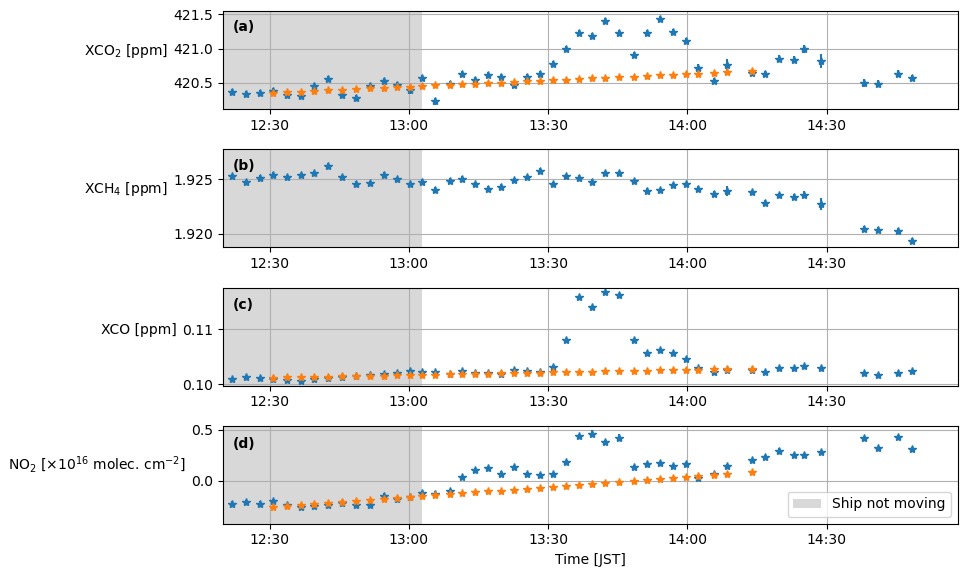
Figure 8 Time series of XCO₂ (a), XCH₄ (b), XCO (c), and NO₂ (d) measured on 13 November 2023 across Mikawa Bay. The estimated background level for the two major plumes is plotted in orange. During the grey-shaded period in the beginning, the ship was in the harbor of Toyohashi. Error bars in all panels show the respective fit uncertainty from the retrieval and reflect precision only.

To investigate the underlying emission patterns for the plumes between 13:30 and 14:00 JST, we calculate enhancements Δ of each species and their enhancement ratios. For this purpose, we remove the background column and convert NO₂ to NO_x to make our results comparable with inventory data and standard emission ratios.

For background removal, we fit a line to the measurements before and after the plume using a least-squares method. Care is taken to exclude from the fit measurements with other enhancements (e.g., in the NO₂ VCD between 13:10 and 13:20 JST). The background level defined by this method is shown in orange in Fig. 8.

To convert NO₂ to NO_x (= NO + NO₂), we use a conversion factor of NO_x/NO₂ =1.32 taken from Beirle et al. (2019), where it has been derived based on the assumption of photostationary steady state. The reasoning in Beirle et al. (2019) and Beirle et al. (2021) suggests that this factor can be applied here, since our measurements are taken at sunny conditions with SZA <65°, the air masses inside the plume are generally polluted and near the surface, and the measurements are taken far enough from the source for the NO-to-NO₂ conversion inside the plume to be roughly in equilibrium. Additionally, Beirle et al. (2021) have calculated the NO-to-NO₂ ratio for various global regions. The annual average for different regions in Japan between 1.25 and 1.45 is close to the global average of 1.32. Because of this, we use this factor in our study, although considerable uncertainties remain.

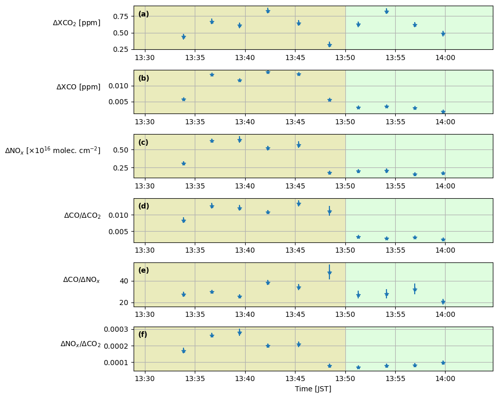
Figure 9 (a–c) Enhancements after the subtraction of the background (marked orange in Fig. 8) in the plumes measured on 13 November 2023. NO₂ has been converted to NO_x using the conversion factor of 1.32 from Beirle et al. (2019). (d–f) Enhancement ratios calculated based on the enhancements shown in panels (a)–(c). The yellow and green background shading refers to episodes A and B as defined in the main text. Error bars in all panels show the respective fit uncertainty from the retrieval and reflect precision only.

Figure 9a–c shows the enhancements Δ of XCO₂, XCO, and NO_x. A clear separation between two distinct episodes is seen with high values in ΔXCO and ΔNO_x before 13:50 JST (episode A, yellow shading in Fig. 9), and low abundances afterwards (episode B, green shading in Fig. 9). In contrast to this, during both episodes, ΔXCO₂ shows a distinct peak. This observation supports the existence of two different air masses with two different sources.

The distinct ΔXCO in episode A is much larger than all other CO enhancements detected throughout the transect (see Fig. 8). It requires a strong, local emitter upwind of the route of the Nichiyu Maru. Figure 10 compares the position of the measured CO-plume to three emission inventories: the Regional Emission inventory in ASia (REAS, version 3) compiled for the year of 2015 (Kurokawa and Ohara, 2020) and two different versions of the Emissions Database for Global Atmospheric Research (EDGAR) compiled for 2018 and 2022 (Crippa et al., 2018, 2024). All three inventories contain a single grid cell with CO emissions being much larger than in all other grid cells. The main CO emission source of this grid cell is listed as “steel manufacturing” in the inventories. In the case of REAS (panel a) and EDGAR v8.1 (panel c), the location of the point source is upwind of the location where our instrument measured the largest enhancement. For EDGAR v6.1 (panel b), the large emitter is displaced by roughly 0.3° longitude to the west, which tends to align worse with our measurements, considering the ERA-5 wind direction. The misplacement of the steel factory in EDGAR v6.1 was indeed confirmed by the EDGAR team (personal communication). This shows the capability of our setup to validate the correct positioning of point sources in inventories.

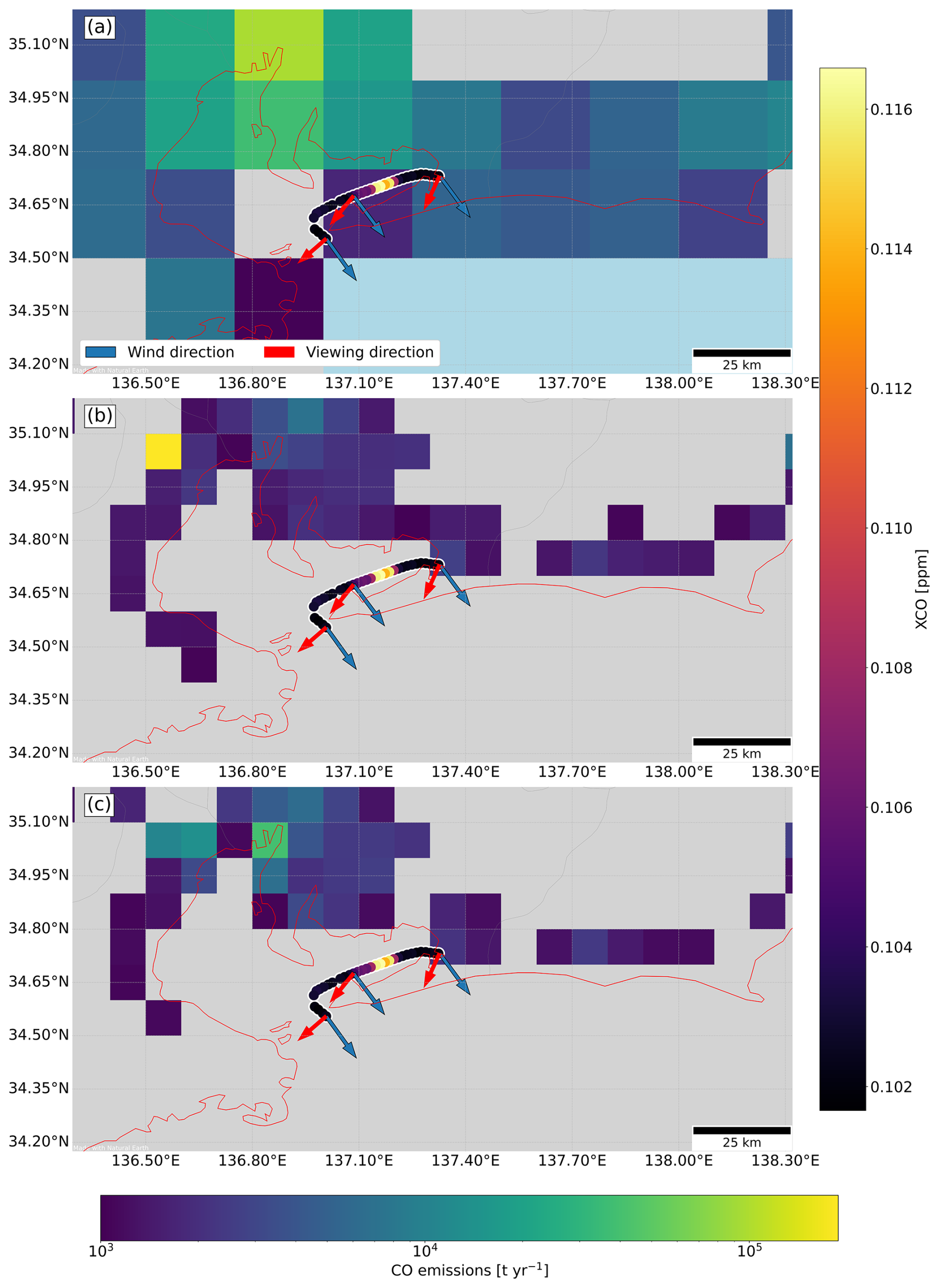
Figure 10 Comparison of measured XCO enhancements to CO emission patterns from different inventories: (a) REAS inventory for 2015 (Kurokawa and Ohara, 2020); (b) EDGAR v6.1 for 2018 (Crippa et al., 2018); (c) EDGAR v8.1 for 2022 (Crippa et al., 2024). Cells with emissions below 1000 t yr⁻¹ according to the respective inventory are shown in grey. Wind directions (blue arrows), interpolated to the location and time of the measurement, are taken from ERA-5 (Hersbach et al., 2020). Viewing direction is shown by the red arrows. Note that the REAS inventory (a) only includes land grid cells.

In order to delve deeper into the origin of the enhancements in episodes A and B shown in Fig. 9, we calculate enhancement ratios from our measurements to compare them to the emission ratios of inventory grid cells or source types. Each source type emits a characteristic ratio of the trace gases CO₂, CO, and NO_x (see Table 7), which can be related to the fuel type as well as the type and efficiency of combustion. Concerning fuel type, for example, lignite coal contains, on average, much less carbon, much more oxygen, and about the same amount of nitrogen as crude oil (Klemm and Hoppe, 1980), leading to a higher NO_x $/$ CO₂-ratio for oil-fired compared to coal-fired power plants (Guevara et al., 2024) through non-linear reaction mechanisms. With respect to combustion efficiency, significant CO emissions are indicative of incomplete combustion (Klemm and Hoppe, 1980), which is typical for biomass burning or steel factory blast furnaces (Zhong et al., 2017; Schneising et al., 2024). Finally, NO_x is also a combustion tracer formed by the highly temperature-dependent Zeldovich mechanism (Zeldovich, 1984) and is therefore indicative of the combustion temperature. The theoretically expected emission ratios are further altered through emission mitigation technologies such as selective catalytic reduction, which removes NO_x from power plant plumes (Srivastava et al., 2005), leading to characteristic emission signatures for different technologies. When comparing emission ratios to enhancement ratios in the atmosphere, various emission contributions can blend due to atmospheric transport and mixing, such that the atmospheric enhancement has contributions from various emission sources.

In order to calculate enhancement ratios from our measurement, we convert the measured column enhancements (in units of vertical column densities (molec. cm⁻²)) into mass enhancements (in units of mass fractions or mass columns (kg cm⁻²)) using the molar mass of the respective species. Then we calculate mass ratios (in units kg kg⁻¹) to compare to the reported emission ratios.

Guevara et al. (2024)Guevara et al. (2024)Guevara et al. (2024)Guevara et al. (2024)Guevara et al. (2024)Schneising et al. (2024)Van der Maas (2019)Liu et al. (2021)Liu et al. (2021)Brown et al. (2014)Fontaras et al. (2014)Park et al. (2021)Kesgin and Vardar (2001)Zhao et al. (2022)Xiao et al. (2022)

Table 7 Overview of the measured enhancements (Δ), emission ratios for different fuel types and sources, and emission ratios taken from the EDGAR inventory (Janssens-Maenhout et al., 2019; Crippa et al., 2024) for the grid cells with the largest point source emitters in the studied region. Source types discussed in the text are marked in bold.

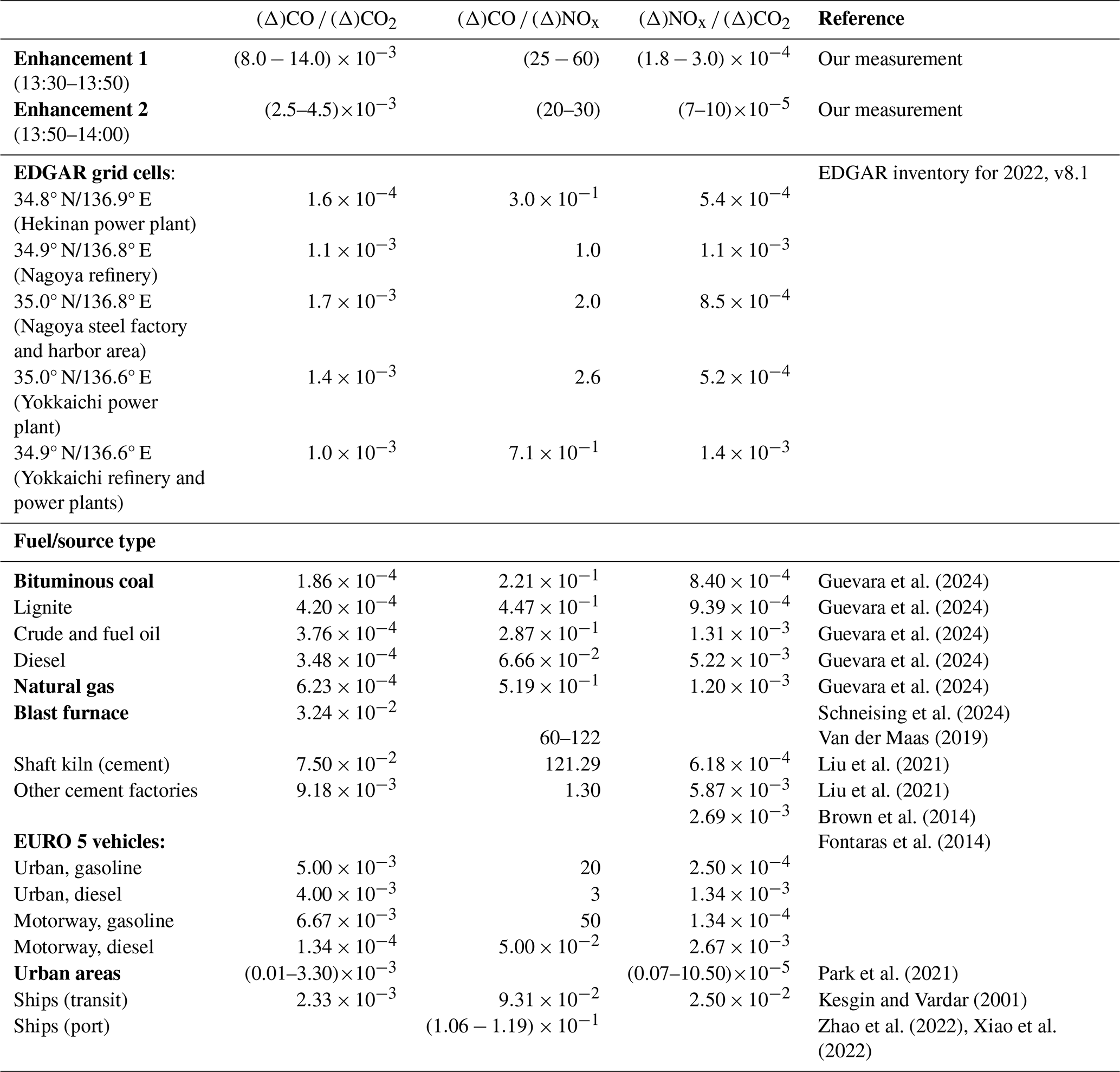
The enhancement ratios measured with our instrument show large differences between the two plume episodes, as can be seen in panels d–f of Fig. 9 and Table 7 (upper rows). During episode A, ΔCO $/$ ΔCO₂, ΔNO_x $/$ ΔCO₂, and ΔCO $/$ ΔNO_x are on average larger than in episode B, suggesting that the emission sources were different for the two episodes. In the following, both episodes are compared separately to the gridded EDGAR inventory and potential source signatures.

The first plume measured between 13:30 and 13:50 JST (episode A; yellow shading in Fig. 9) has a ΔCO $/$ ΔCO₂ of (8.0–14.0)$\times {\mathrm{10}}^{-\mathrm{3}}$, a ΔCO $/$ ΔNO_x of 25–60 and a ΔNO_x $/$ ΔCO₂ of (1.8–3.0)$\times {\mathrm{10}}^{-\mathrm{4}}$. If this is compared to the emission ratios of the EDGAR grid cells containing large emitters listed in the upper part of Table 7, the measured ΔNO_x $/$ ΔCO₂ is found a factor 2 or more lower, and the measured ΔCO $/$ ΔCO₂ as well as the measured ΔCO $/$ ΔNO_x are a factor 5 to 10 larger than the emission ratios in all EDGAR grid cells.

As pointed out previously, the large CO content of the plume in episode A suggests a steel factory as an important contributor. Other source types with large CO emissions (see Table 7), such as shaft kilns from the cement industry or motorways, can be ruled out based on Climate TRACE coalition (2022). According to a new study based on satellite data (Schneising et al., 2024), blast furnace steel production can lead to CO $/$ CO₂ emission ratios of $\mathrm{3.24}\times {\mathrm{10}}^{-\mathrm{2}}$ on average, being larger than our measured enhancements by a factor of 2 to 3. While our measured ratios are lower than typical blast furnace CO $/$ CO₂ ratios, the presence of the Nippon Steel Nagoya factory, operating two large blast furnaces and two basic-oxygen furnaces (Nippon Steel Corporation, 2024), indicates that steel production is a plausible, important contributor. Also, the large ΔCO $/$ ΔNO_x enhancement ratios are, by a factor of 2 to 4, smaller than ratios expected for steel factories (Van der Maas, 2019) (see also Table 7). For steel factories, Van der Maas (2019) found a CO $/$ NO_x emission ratio between 60 and 122 based on data from the TROPOMI satellite for five blast furnaces. They point out that these findings disagree by up to one order of magnitude with the EDGAR v6.1 inventory (Crippa et al., 2018; Janssens-Maenhout et al., 2019), which reports emission ratios between 2.8 and 16.8 for the same blast furnaces. This discrepancy is partly attributed to EDGAR relying on end-of-pipe measurements at the chimney and not including fugitive emissions within steel factories. Based on the emission ratios found by Van der Maas (2019) and Schneising et al. (2024), a blast furnace as the major source, with mixing from other sources with lower CO content, would fit our measured enhancement ratio quite well. The low measured NO_x $/$ CO₂ ratio might point at mixing of the steel factory plume with air masses carrying low NO_x $/$ CO₂ ratios, such as caused by traffic ($\mathrm{2.5}\times {\mathrm{10}}^{-\mathrm{4}}$ (Fontaras et al., 2014), assuming EURO 5 engines, urban driving conditions, and a vehicle fleet dominated by gasoline engines, which is typical for Japan (IEA-AMF, 2023)) or gas-fired power plants. Indeed, the city center of Nagoya, with a high traffic density, and several gas-fired power plants are located in the vicinity of the steel factory (Climate TRACE coalition, 2022). The latter are equipped with low-NO_x burners or denitration equipment (Jera Corporation, 2025), which reduces the NO_x $/$ CO₂ ratio of a gas-fired power plant listed in Table 7 by up to 90 % (Crippa et al., 2018). Although the EDGAR inventory at the grid cell level cannot fully explain the enhancement signature of episode A, a fitting source composition dominated by steel factory emissions and contributions from gas-fired power plants with low-NO_x burners and traffic can be found based on the measured enhancement ratios.

Episode B (green shading in Fig. 9) of the plume detected after 13:50 JST contains much less CO and NO_x than episode A, implying lower ΔCO $/$ ΔCO₂ and ΔNO_x $/$ ΔCO₂ enhancement ratios (see Table 7). This hints at a different source composition than for episode A. From the approximate wind direction shown in Fig. 7, the coal-fired Hekinan power plant, one of the largest in Japan (Climate TRACE coalition, 2022), and the two smaller co-located coal-fired power stations, Taketoyo and Nagoya, appear to be likely sources. Other large emitters in the Nagoya region, such as the Yokkaichi power plant, are located upwind of these three power plants as seen from the ship's position and may, therefore, also partly contribute.

Based on the EDGAR inventory (Crippa et al., 2024), the grid cell containing these three large coal-fired power plants should have a CO $/$ CO₂ emission ratio of $\mathrm{1.6}\times {\mathrm{10}}^{-\mathrm{4}}$, a CO $/$ NO_x emission ratio of 0.3, and a NO_x $/$ CO₂ emission ratio of $\mathrm{5.4}\times {\mathrm{10}}^{-\mathrm{4}}$. The measured enhancement ratios ΔCO $/$ ΔCO₂ of (2.5–4.5)$\times {\mathrm{10}}^{-\mathrm{3}}$ and ΔCO $/$ ΔNO_x of 20–30 are however considerably larger and the enhancement ratio ΔNO_x $/$ ΔCO₂ of (7–10)$\times {\mathrm{10}}^{-\mathrm{5}}$ is considerably smaller than the respective emission ratios of the EDGAR grid cell containing the power plants. Part of the discrepancy between EDGAR and our measurement can, however, be explained by the Taketoyo power plant as well as one out of two units of the Nagoya power plant and three out of five units of the Hekinan power plant being switched off for maintenance or due to technical failures (Japan Electric Power Exchange, 2024). Because of this, other co-located sources with different emission ratios, such as traffic, are expected to contribute relatively more to the measured enhancement ratios. Therefore, our measurements are not expected to match the emission ratios from EDGAR. Indeed, the city center of Nagoya is located approximately upwind of our measurement from Hekinan. A study on urban emission ratios based on satellite data by Park et al. (2021) showed that urban areas of selected cities of different sizes in the northern hemisphere have emission signatures similar to our measured enhancement ratios (see Table 7). Episode B illustrates that while EDGAR and other inventories typically provide annual emission data, regular ship-based measurements can be used to inform on the temporal profiles of emissions and irregular emission behavior, such as shutdowns. This showcases the advantage of our instantaneous measurements, which can be used to infer irregular emission patterns, in contrast to the bottom-up approach of inventories such as EDGAR, relying solely on annual means.

The current study is limited by the approximate use of wind directions from the ERA-5 reanalysis (Hersbach et al., 2020), which is possible here because of the closely located sources and a very uniform wind field. These conditions are, of course, not warranted during all days of the deployment, and especially scenarios where the ship is further away from emission sources are of large scientific interest. To study such sources, the usage of wind trajectory models such as FLEXPART (Pisso et al., 2019) is needed. An optimized analysis framework including such trajectories is currently under development.

6 Conclusion and outlook

We have developed an autonomous multi-species mobile spectrometer setup consisting of an EM27/SUN FTS for the shortwave-infrared and a DOAS grating spectrometer for the visible wavelength range, both using direct sunlight as a light source. This setup has been successfully deployed and operated without permanent human attendance over several months on a commercial vessel traveling along the coast of Japan. The setup allows for measuring column abundances of CO₂, CH₄, CO, and NO₂ with high precision and repeatability. The latter has been tracked through regular side-by-side measurements with a spectrometer of the COCCON. This shows that our shipborne measurements of CO₂, CH₄, and CO are compatible with the standards of the COCCON and, in consequence, they can be adjusted to the TCCON scale through a multiplicative adjustment. Thus, our setup is suitable for several potential use cases.

Here, we have demonstrated, in a case study, the detection of plume enhancements of ΔCO₂, ΔCO, and ΔNO₂, carrying the outflow from the heavily populated Nagoya region. Converting ΔNO₂ into ΔNO_x under assumption of photochemical steady state, the enhancement ratios ΔCO $/$ ΔCO₂, ΔNO_x $/$ ΔCO₂, and ΔCO $/$ ΔNO_x, together with wind information, suggest that the first episode of the plume originates mainly from a steel factory while the second episode most likely relates to emissions from coal-fired power plants and sources of urban signature. Comparing these findings to emission inventories such as EDGAR, we find that the gridded emissions and their ratios can be successfully checked using routine shipborne measurements. Due to the multi-species system, a source-sensitive assessment is feasible, which is especially valuable in regions of densely spaced emitters. Building on the demonstrated potential of the instrument, long-term shipborne installations will enable systematic emission monitoring along coastal hotspots.

A second use case is satellite validation over open oceans, where almost no data currently exists (Müller et al., 2021). This use case has already been demonstrated for a shipborne FTS in our previous publications (Klappenbach et al., 2015; Knapp et al., 2021),where the system still required on-board personnel. Having now an upgraded instrument that can operate fully remotely for several weeks and that is compatible with COCCON standards, as demonstrated within this study, makes future routine deployments for satellite validation over the open ocean possible. In addition, the added capability to simultaneously measure NO₂ makes our instrument an ideal platform for the validation of the newest generation of satellites measuring this air pollutant along with the greenhouse gases, if an appropriate route for the ship is chosen.