An adaptive segmentation approach for contrail detection in meteosat second generation satellite imagery

Line-shaped ice clouds known as contrails are produced by aircraft and play a notable role in aviation’s contribution to climate change. One promising and cost-effective approach to mitigating this impact is the operational avoidance of contrail formation. To enable the design and evaluation of such mitigation strategies, reliable automated detection of contrails using spaceborne geostationary sensors is essential. In this work, we present a contrail detection algorithm named COCOS (Contrail Confidence Score) for the Meteosat Second Generation (MSG) satellite. Contrail detection with MSG is challenging due to its moderate spatial resolution of 3 km at nadir. COCOS uses a combination of image processing techniques to identify line-shaped contrails. An adaptive thresholding technique as well as a new object separation method and advanced false alarm reduction procedures are implemented. Furthermore, instead of returning just a binary contrail mask as a result, COCOS returns a confidence score to indicate the degree of certainty of each contrail identification. COCOS is evaluated based on a human-labeled dataset. It comprises 140 images of 256 × 256 pixels from 2013–2024, about 60 % of which contain contrails according to human labelers, covering the entire MSG disk with a higher concentration over Europe and the North Atlantic flight corridor. COCOS outperforms the other known contrail detection algorithms in the literature for MSG. At similar recalls (the fraction of true positives correctly identified) it achieves precisions (the fraction of positive predictions that are correct) more than three times higher (0.65 for recall 0.25 and 0.3 for recall 0.5) than other MSG-based contrail detection algorithms, providing a significant improvement in contrail detection for MSG.

1 Introduction

Contrails are thin ice clouds created by aircraft when the ambient temperature is low enough. When the ambient air is supersaturated with respect to ice, contrails can persist for hours (e.g., Lewellen, 2014; Vázquez-Navarro et al., 2015) and, through spreading and ice crystal growth, can transition into contrail-induced cirrus clouds. Aviation contributes approximately 3.5 % to total anthropogenic effective radiative forcing (ERF), with contrail cirrus estimated to be the largest contributor, surpassing even aviation CO₂ emissions in their impact (Lee et al., 2021). Modeling studies have shown that a large fraction of the contrail cirrus radiative forcing can be attributed to few contrail outbreaks (Burkhardt et al., 2018), with only a small number of flights being responsible for a disproportionate share of the contrail related climate impact, highlighting the potential for targeted mitigation (e.g. Teoh et al., 2024). However, observational evidence about the properties and radiative effects of these events remains limited. To advance knowledge in this area, passive imaging observations from geostationary satellites are an important tool since they enable the identification of contrails and the estimation of their radiative effect along their life cycle (e.g., Sonabend-W et al., 2026; Mannstein and Schumann, 2005; Chevallier et al., 2023; Wang et al., 2023, 2024; Vázquez-Navarro et al., 2015; Haywood et al., 2009; Atlas et al., 2006). Furthermore, passive remote sensing can provide a relevant contribution to monitor contrail formation in contrail mitigation strategies. In particular, one promising and cost-effective mitigation strategy is contrail avoidance by rerouting flights to avoid regions where contrails are formed (Sausen et al., 2023) and/or where warming contrails can persist (Sonabend-W et al., 2024; Geraedts et al., 2024; Frias et al., 2024; Sarna et al., 2025). These warming contrail regions are forecast with numerical contrail models fed with numerical weather prediction model output (Schumann, 2012; Engberg et al., 2025; Yin et al., 2023). Automatic contrail detection in satellite imagery enhances the effectiveness and efficiency of the aviation industry's climate actions by providing means to evaluate (a) the relative humidity over ice in the upper troposphere in the NWP models (e.g., Wolf et al., 2025; Wang et al., 2025; Teoh et al., 2022); (b) contrail models in general (e.g., Schumann, 2012; Fritz et al., 2020; Verma and Burkhardt, 2022; Yin et al., 2023); and (c) the success of contrail mitigation strategies (as e.g. in Sausen et al., 2023; Sonabend-W et al., 2024), while also contributing to climate mitigation efforts. The potential of brightness temperature difference images for identifying thin cirrus clouds composed of small ice particles was recognized early on (Inoue, 1985). Contrail detection in satellite images has been studied for more than three decades, with the earliest detections carried out manually in polar orbiting satellite observations (e.g., Bakan et al., 1994). Building on these foundations, Mannstein et al. (1999) presented the first automatic linear ice cloud detection for the Advanced Very High Resolution Radiometer (AVHRR). Earlier contrail detection methods were mainly proposed for low-Earth-orbit satellites, as they had a better spatial resolution than geostationary sensors (Mannstein et al., 1999; Minnis et al., 2013; Bedka et al., 2013; Duda et al., 2013; Vázquez-Navarro et al., 2015), and because they also carried suitable spectral channels to achieve this task. However, they have the disadvantage of low temporal resolution. Geostationary satellites provide high temporal and spatial coverage, but come with moderate spatial resolution, which makes contrail detection more difficult. It has been proven that linear contrail detection works reasonably well with geostationary satellites of the current generation like Geostationary Operational Environmental Satellite GOES-R/S/T (Zhang et al., 2018; Meijer et al., 2022; Chevallier et al., 2023; Ng et al., 2024). Since contrails that can be observed in geostationary imagers are also those with a larger radiative impact, satellite detection remains a valuable tool despite limited overall observability (Driver et al., 2025). Recent advances in the field of artificial intelligence and machine learning have enabled contrail detection algorithms using artificial neural networks, mainly focusing on geostationary satellites observing the North and South America (Zhang et al., 2018; Kulik, 2019; Meijer et al., 2022; Chevallier et al., 2023; Ng et al., 2024). They show that machine learning is a valuable tool for image detection tasks. In this work, a new linear contrail detection algorithm for the Spinning Enhanced Visible and Infra-Red Imager (SEVIRI) aboard the Meteosat Second Generation (MSG) satellite is presented. Contrail detection with MSG/SEVIRI over Europe, which due to its high air traffic density is a relevant area when investigating climate effects of aviation (Teoh et al., 2024), has been done using adapted versions (Mannstein et al., 2010; Dekoutsidis et al., 2023) of the algorithm presented by Mannstein et al. (1999). However, detection efficiency is low due to the challenges posed by SEVIRI's spatial resolution, with less than 50 % of contrails being detected. We propose an algorithm named COCOS that leverages the broad spectral coverage provided by the numerous channels of MSG. It uses new methods like adaptive thresholding and an advanced technique to separate individual linear objects. In contrast to other algorithms previously used for MSG, it can be tailored for a range of applications by choosing a desired contrail confidence score, i.e. a threshold that expresses different trade-offs between precision and recall. Existing automatic algorithms for MSG produce pixel-wise binary outputs and are limited in flexibility; our approach fills this gap by offering an adaptable, object-based method that improves detection and reduces false alarms. By prioritizing a physically based, rule-driven logic over an end-to-end machine learning architecture, the authors aim to facilitate the future adaptation of COCOS to the Meteosat Third Generation satellite. Furthermore, we gain a deeper understanding of the factors affecting contrail detection – such as why a contrail is detected or missed, which spectral channels contribute most, and which contrail characteristics are most informative, thereby strengthening the use of COCOS for assessing temporal and spatial contrail distributions, evaluating the effectiveness of mitigation strategies (such as flight rerouting), and improving the representation of aviation-induced clouds in climate models and contrail models. This paper is structured as follows: We begin by presenting the MSG data and relevant channels in Sect. 2, reviewing previous contrail detection methods, introducing two cloud retrieval algorithms, describing the labeled contrail dataset used for training and testing, and describing the evaluation metrics applied. Next, we provide a detailed description of the new contrail detection approach in Sect. 3, including an explanation of the underlying methods and a representative example of the algorithm’s output. We then evaluate the algorithm's performance by comparing its recall and precision to existing contrail detection methods for MSG in Sect. 4.1. Additionally, in Sect. 4.3 we examine how contrail and background scene properties influence detection performance. Finally, in Sect. 5 we summarize the main findings and discuss their implications for future research on contrail detection and characterization.

2 Data and Methods

2.1 MSG/SEVIRI

The Meteosat Second Generation (MSG) satellite (Schmetz et al., 2002) carries the SEVIRI radiometer. The MSG program consists of a series of four geostationary satellites (MET-8 to MET-11), primarily operated at the nominal 0°E longitude to provide observations over Europe and Africa, with additional instances positioned at other longitudes or operated in different modes. SEVIRI acquires images every 15 min, with a spatial resolution of 3 km at nadir and roughly 4–6 km over Europe due to the oblique viewing geometry. SEVIRI has twelve spectral channels, four in the solar spectrum to measure reflected solar radiation and eight in the infrared spectrum to observe emitted thermal radiation. Given that contrails are poorly visible in solar channels, and therefore their consideration is not expected to substantially enhance detection – though this possibility was not formally examined in this work – only infrared channels are used in this work. This also ensures that contrail detection remains possible throughout the day. In the following, all channels will be referenced by their central wavelength (e.g. IR108 for the infrared channel centered at 10.8 µm).

2.2 Cloud Remote Sensing with MSG/SEVIRI

Two cloud algorithms for MSG/SEVIRI are used in this work. The CiPS (Cirrus Properties from SEVIRI) retrieval algorithm detects ice clouds and estimates their properties (Strandgren et al., 2017a). It uses four artificial neural networks to retrieve ice cloud properties using data from MSG/SEVIRI, surface temperature data and other auxiliary data. CiPS was trained with Cloud-Aerosol Lidar with Orthogonal Polarization (CALIOP) cloud products collocated with MSG observations. Properties provided by CiPS include a cirrus cloud flag, a cirrus opacity flag, ice optical thickness, cloud top height, ice water path and effective radius. The cirrus cloud flag can be interpreted as a cirrus probability. Based on the comparison of CiPS to 4.9 million CALIOP collocations, it has a detection accuracy of 71 % and 95 % of cirrus clouds with an optical thickness of 0.1 and 1, respectively. It has a relative error of less than 10 % regarding cloud top height and mean absolute percentage error of less than 100 % for ice optical thickness and ice water path. A thorough evaluation can be found in Strandgren et al. (2017b). CiPS is a powerful tool for analyzing the temporal evolution of cirrus clouds including their optical and physical properties (see e.g. Rybka et al., 2021; Wang et al., 2023).

The second algorithm is the ProPS retrieval for cloud-top phase determination for MSG/SEVIRI (Mayer et al., 2024a). It uses a Bayesian approach based on collocations between MSG/SEVIRI observations and the DARDAR cloud product (Ceccaldi et al., 2013; Mayer et al., 2023) to distinguish five classes of cloud-top phase: warm liquid, supercooled liquid, mixed-phase, thin ice and thick ice. Validation of ProPS with six months of DARDAR observations demonstrated high skill, correctly identifying 93 % of clouds, 86 % of clear-sky pixels, and achieving classification accuracies of up to 91 % for ice clouds.

2.3 Contrail Remote Sensing with MSG/SEVIRI

Contrail detection in MSG imagery poses several challenges. One major limitation is the relatively low spatial resolution of 3 km at nadir, which makes it difficult to identify thin, newly formed contrails. In mid-latitudes the spatial resolution is even lower around 4–6 km. By the time contrails are captured in MSG images, they are often older and have spread out, appearing broader and less distinct, which further complicates detection. Gierens and Vázquez-Navarro (2018) suggest that the average age of a contrail at the time of its first detection in MSG is 1.5 h, assuming a spreading rate of 5 km h⁻¹. In satellites with a better spatial resolution like GOES (2 km at nadir), contrails can be observed over the US as early as 20 min after their formation (Geraedts et al., 2024). Additionally, persistent contrails can merge with natural cirrus clouds, making it challenging to distinguish anthropogenic features from the background cloud field. Furthermore, especially with the spatial resolution of MSG/SEVIRI, natural clouds can also show linear features that are difficult to distinguish from contrails (Unterstrasser et al., 2017b). Finally, variability in illumination, atmospheric conditions, and underlying cloud cover also affect the contrast and visibility of contrails. SEVIRI, with its eight thermal channels, offers various possibilities to investigate ice clouds and contrails. Six SEVIRI channels are mostly used in this work and described further. The IR039 channel, centered at 3.9 µm in the shortwave infrared, is sensitive to both reflected solar radiation during daytime and thermal emission at night, making it useful for detecting low-level clouds, fog, and contrails (Schmetz et al., 2002). Especially during daytime it is sensitive to the cloud phase and very sensitive to the particle size, which can help to distinguish contrails from natural cirrus (Inoue, 1985) since contrails consist of smaller ice particles in the contrail core (e.g. Voigt et al., 2010, 2017; Unterstrasser et al., 2017a, b). WV062 and WV073 are the water vapor channels of SEVIRI. They are centered at 6.2 and 7.3 µm, respectively, in the water vapor absorption band, with absorption intensity being higher at the former wavelength. WV062 is thus more sensitive to upper tropospheric water vapor, while WV073 samples lower atmospheric layers (Schmetz et al., 2002). The WV062 channel shows high-altitude water vapor features more clearly due to its strong upper-tropospheric sensitivity, but the contrail-background contrast can be larger in WV073, since it senses relatively warmer radiation from below that is blocked by the contrail. The brightness temperature difference (BTD) between these two indicates the amount of high level moisture and can also be used for ice cloud detection (Krebs et al., 2007). The three infrared window channels IR087, IR108 and IR120 centered at 8.7, 10.8 and 12.0 µm, respectively, are used to extract high thin cirrus information from satellite observations. Especially the BTDs of those channels help identifying contrails: Due to wavelength dependent absorption and scattering (Rosenfeld and Woodley, 2003; Mayer et al., 2024b), the amount of transmitted radiation through optically thin ice clouds is different for the infrared window channels. This leads to large BTD values compared to optically thick clouds (Gothe and Graßl, 1993). This effect is especially large for ice clouds with small effective radii, which are typical for newly formed contrails (Voigt et al., 2011, 2021), making the contrails stand out relative to other clouds in BTD images. For instance, Mannstein et al. (1999) has used two channels corresponding to 10.8 and 12.0 µm to highlight and detect contrails (IR087 was not available at that time), while newer contrail detection algorithms rely on all three infrared window channels (e.g. Ng et al., 2024). In this paragraph, the contrail detection algorithm proposed by Mannstein et al. (1999) is described briefly, as adaptations of this method represent the current standard for contrail detection in MSG and we compare COCOS to them in a later section. The detection scheme of Mannstein et al. (1999) was originally developed for the Advanced Very High Resolution Radiometer (AVHRR) aboard the National Oceanic and Atmospheric Administration (NOAA) satellites and uses two channels corresponding to 10.8 and 12.0 µm. A normalization procedure using rotationally symmetric Gaussian 5 × 5 kernels is applied to generate a single normalized high-pass filtered image, ensuring comparable contrast and consistent thresholding in different meteorological conditions. Two normalized images for the (inverted) brightness temperatures (BTs) at 12.0 µm and the BTD 10.8–12.0 µm are first computed separately as the difference between the original and the smoothed image with this Gaussian kernel, and are normalized with their so called local standard deviation. In a second step, the sum of these two normalized images (contrails are cold and have thus high values in the inverted BT that enhance the high BTD values) produces the picture that is used for contrail detection. Pixels belonging to line-shaped objects are extracted from this normalized image by applying line filters of 19 × 19 pixels in 16 different line inclinations (0 … 180°). To distinguish between real contrails and other linear features (cloud edges or structures, coastlines, …), for every inclination a set of criteria are evaluated on a pixel and object basis: (a) Contrails are assumed to correspond to bright pixels in the normalized image; (b) The BTD IR108 – IR120 must be large enough; (c) An upper limit on the large-scale gradient of the IR120 BT, depending on the regional standard deviation, eliminates cloud edges and sometimes shorelines that also show up as lines in the normalized image. This large-scale maximum gradient of IR120 is calculated by convolving the BT IR120 image with a 15 × 15 Gaussian kernel and determining the derivatives in x and y direction as the difference between neighboring points. The gradient is then computed by combining the derivatives in the x and y directions; (d) Object properties (number of pixels, length and correlation of pixels to a straight line) are finally evaluated and too small or too non-linear contrails are removed from the detection results. The results from all directions are combined to produce the final binary contrail mask. For more details please see Mannstein et al. (1999).

The literature contains four adaptations of this algorithm that aim to detect contrails in MSG which will later be compared to COCOS: (a) the original Mannstein et al. (1999) algorithm, applied to the IR108 and IR120 channels, that looks for contrails in 32 different directions (in the following called M108); (b) the algorithm used in Mannstein et al. (2010) that utilizes the IR087 and IR120 channels for 32 different directions (in the following called M087); (c) a combined version of the previous two that uses the BTD between IR087 and IR120 and the BTD between IR108 and IR120 with some additional features (two different line filter sizes 17 and 19 are used together with 32 line directions), in the following called Mcomb; (d) the algorithm by Dekoutsidis et al. (2023) where IR108, IR120 and WV073 are used.

2.4 Contrail Ground Truth

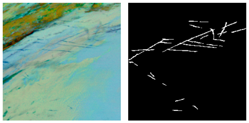
A labeled contrail dataset (Santos Gabriel et al., 2026) is used to develop and evaluate COCOS. The dataset contains 140 labeled MSG scenes of 256 × 256 pixels. Scenes are randomly distributed geographically across the SEVIRI disk, with clusters of higher density over Europe and the North Atlantic. The time range considered is from 2013 through 2024 and only scenes from MSG3 are used. 60 % of the scenes contain contrails, while the rest remains contrail-free. Labelers received a labeling guide on how to identify contrails in satellite imagery and were asked to mark each individual pixel of a contrail. As additional information the labelers received a time series of different RGB composites and brightness temperature images spanning one hour prior to the target image and one hour following the target image. Each scene was labeled by three individuals, and the ground truth was defined as their majority consensus: if at least two out of three labelers marked a pixel, it was considered a contrail pixel. This ground truth is still subjective and cannot be regarded as perfectly accurate. One example scene is shown in Fig. 1. 51 of the images were employed for the development of COCOS (in the following called training dataset) and 89 images were set aside for later evaluation of the algorithm (in the following called evaluation dataset), ensuring equivalent statistics for both subsets (same distributions of solar zenith angles, number of contrails, …).

Figure 1 Example of an Ash RGB and the ground truth from the human-labeled contrail dataset.

3 Contrail Detection Algorithm

COCOS uses image processing techniques and segmentation to identify line-shaped contrails. Its strategy combines the general approach of Mannstein et al. (1999) to detect contrails in normalized images and then discard false detections, and the idea of using Ash RGBs from recent AI-based contrail detection algorithms (like e.g. Ng et al., 2024), thus exploiting more spectral information. However, COCOS introduces a completely different image processing approach than Mannstein et al. (1999), considers cloud property retrievals to suppress false alarms and finally produces a confidence score for the contrail classification (instead of a binary decision) by “learning” contrail probabilities from the training dataset.

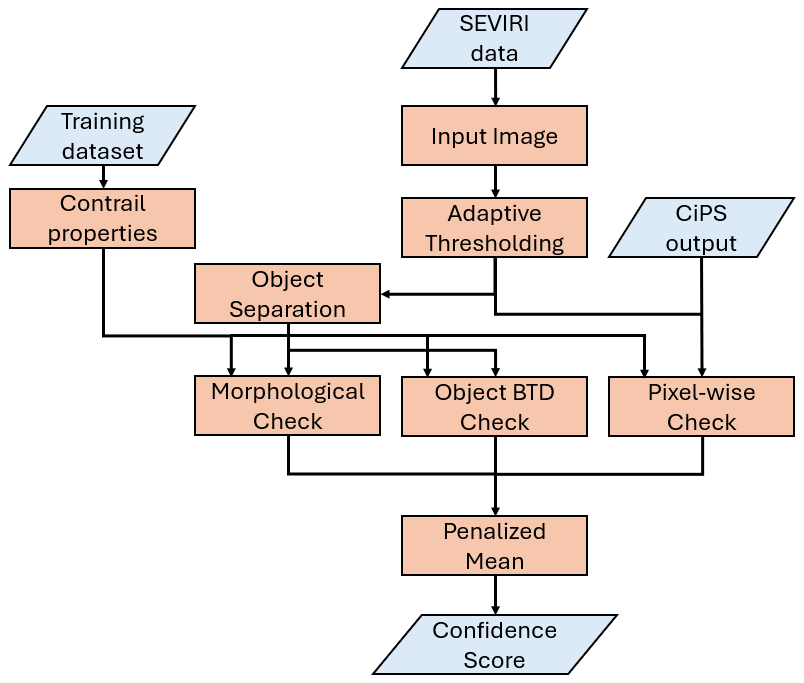
The approach is sketched in the following (see also the flow chart in Fig. 2) and detailed in Sect. 3.1–3.6. Our algorithm creates an input image as a combination of BTs and BTDs and then identifies all bright pixels. Since not all bright pixels are contrails, a part of them must then be removed, as in Mannstein et al. (1999). To this end, the pixels found in this binary mask are grouped into line-shaped objects (if linearity can be found); we call this step Object Separation. Subsequently, three parallel evaluation steps are conducted to determine the contrail confidence. In the first step, contrail properties like cloud top height and BTDs are computed pixel-wise. In the other two steps properties are calculated object-wise. In the second step, morphological properties of the objects are investigated, while in the third step, the difference of the mean BTDs of contrails and the mean BTDs of their surrounding are evaluated. Confidence scores are assigned to each contrail candidate based on confidence functions derived from the training dataset, applied separately across the different property groups. These scores are then combined into a final confidence score using a penalized mean. By selecting different confidence thresholds, various binary contrail masks can be generated with different precision-recall pairs. In the following, the algorithm is illustrated using the example image (Fig. 1). Here several contrails can be observed as dark blue lines in different directions and of different length and contrast. In the upper left corner, a natural ice cloud is present (brown colors). One edge of the cloud looks like a black thick line, representing a very cold cloud top. Further down, on the left border of the image, another dark object with linear edges and an inclination of approx. 45° is visible, which could be part of a natural ice cloud. The yellowish colors, especially in the lower left portion of the picture, represent low-level liquid clouds. The light blue color represents cloud-free areas, e.g., on the right hand side of the image.

Figure 2 Scheme of the contrail detection algorithm COCOS.

3.1 Input Image

In the first step of the algorithm an image is created where contrails are enhanced (Fig. 3a). For this, three SEVIRI channels are used – IR087, IR108 and IR120 – that are also used in EUMETSAT's Ash RGB composite and, e.g., in Ng et al. (2024). These channels are selected as the ice crystals in the optically thin contrails have low effective radii and thus show high BTDs in these infrared channels (see Sect. 2.3). The BTDs IR108 – IR120 and IR087 – IR108 as well as the BT IR108 are normalized to [0, 1] in agreement with EUMETSAT user manual (Table 1).

Table 1 Channels and normalization ranges for Ash RGB according to EUMETSAT user manual. Gamma correction is not applied (γ=1) in this scheme.

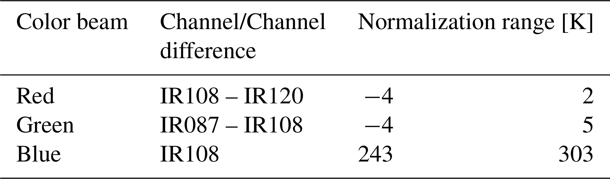
To create the input image, the three normalized components are summed up and the result is normalized to the values between 0 and 1 using minimum and maximum values in each image (making this normalization procedure scene-dependent). This is done to ensure comparable values throughout all images while allowing different scene dependent enhancements for different cloud, temperature and contrail conditions. In this grayscale image, contrails appear as white linear features; however, other bright features, such as natural ice clouds, cirrus streaks, and highly emissive aerosol plumes like hot volcanic ash or industrial smoke, can also produce similar brightness, complicating the identification of contrails. The following sections describe the detection procedure, including how these false features are distinguished and filtered out.

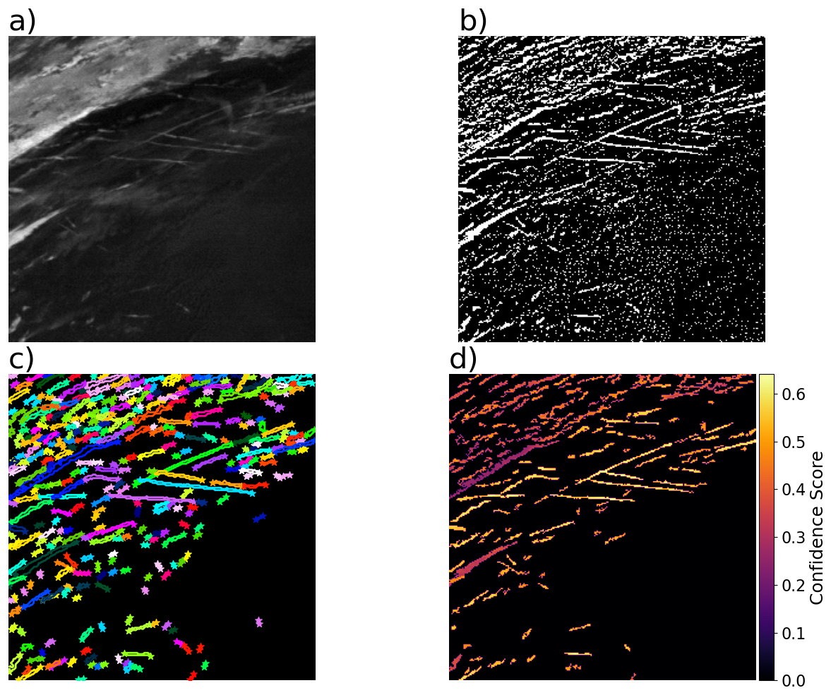
Figure 3 (a) Example Input Image for COCOS. It is derived from the aggregation of the normalized BTDs IR108 – IR120 and IR087 – IR108 as well as the channel IR108; (b) adaptive thresholding for the example image; (c) separated line-shaped objects (this is illustrated by each object being displayed in a distinct color); (d) Contrail confidence score for the example image.

3.2 Adaptive Thresholding

To extract bright features like contrails from the input image, an adaptive thresholding is performed using the OpenCV python library. Unlike global thresholding, adaptive thresholding computes the threshold for each pixel based on its surrounding neighborhood. Here, a Gaussian weighted sum is used, stressing the importance in the center of the kernel, as it typically results in local contrast adaptation and smoother thresholds. The threshold T(x,y) for each pixel (x,y) is calculated based on the Gaussian weighted sum of its local neighborhood 𝒩(x,y) defined by a given window size and a constant C:

$$\begin{array}{}\text{(1)}& T(x,y)=\sum _{(i,j)\in \mathcal{N}(x,y)}G(i-x,j-y)\cdot I(i,j)-C\end{array}$$

where $G(i-x,j-y)$ is the weight from a 2D Gaussian kernel normalized to 1 centered at (x,y) and I(i,j) is the pixel intensity at the pixel (i,j). For this contrail detection algorithm, we compute the Gaussian weighted sum of the 9 × 9-neighborhood and C=4 is subtracted from it. 9 pixels at mid-latitudes correspond to about 36–45 km in S–N direction, which is much larger than the typical width of contrails found in Vázquez-Navarro et al. (2015). Here, a neighborhood 𝒩 of 9×9 pixels and C=4 are selected based on iterative testing. Subtracting C fine-tunes the threshold, allowing pixels slightly darker than the local mean to be selected in homogeneous regions. A binary mask – called AT in the following – (see Fig. 3b) based on the comparison of the pixel value I(x,y) and its threshold T(x,y) is derived:

$$\begin{array}{}\text{(2)}& \mathrm{AT}(x,y)=\left\{\begin{array}{ll}\mathrm{1},& \text{if }I(x,y)>T(x,y)\\ \mathrm{0},& \text{otherwise}\end{array}\right.\end{array}$$

The adaptive thresholding ensures a robust identification of bright features, including contrails, across different image conditions, independent of the specific scene or context. Even low contrasted objects (contrails) can be extracted with this method (see e.g. features in the lower part of Figs. 1, 3a and b), independent of linearity. Compared to edge detection algorithms (e.g. Canny, 1986; SOBEL, 1970), it can detect not only thin lines (e.g., the two edges of a contrail separately) but wider objects as a whole. However, many small objects (see lower right part of Fig. 3b) and objects with holes (see upper part of Fig. 3b) are produced this way. The binary mask AT produced this way contains many small and large objects that are only in part contrails. Thus, this mask is analyzed in three ways in the next section to assign a confidence value for contrails. On one side, pixel-wise properties are investigated; on the other side, objects are produced from the result of the adaptive thresholding and characteristics of these resulting objects are then examined in two ways. The operations are carried out interdependently on the binary mask AT produced by the adaptive thresholding step, after which the outcomes are integrated.

3.3 Confidence Functions

The analysis of the binary mask produced by the adaptive thresholding is performed with the help of confidence functions derived from the training dataset (see Sect. 2.4). Note that the function referred to here as a confidence function is not a true probability density – its integral is not necessarily one – but rather represents the fraction of true positives relative to the total number of positives. In this dataset, objects are identified after adaptive thresholding and separated into contrail and non-contrail objects based on the ground truth. We generate smoothed density functions for the following properties: pixel-wise CiPS properties (cirrus cloud probability, cirrus opacity probability, cloud top height, ice optical thickness, ice water path, ice crystal effective radius), large-scale maximum gradient of BT IR120 (see Sect. 2.3), BTD IR108-IR120, BTD WV062-WV073 and BT IR039; object-wise length, mean width, maximum width, standard deviation of widths, linearity and number of holes; differences of mean BTD of objects to their direct surrounding (defined as all pixels within a maximum 2-pixel border around the object, obtained by performing a binary dilation) using four BTDs, namely IR087 – IR108, IR039 – WV062, IR108 – IR120 and WV062 – WV073. The width is defined as twice the perpendicular distance from a pixel to the line. A Principal Component Analysis (Hotelling, 1933) is performed, and the proportion of variance explained from the first component is used as a linearity score for the objects. If the pixels form a line, most variance is captured by the first principal component; if they form a blob, variance is shared with the second. Thus, the variance fraction of the first component serves as a linearity score. This method is used to assess linearity of contrails as it is robust with respect to the coordinate system, unlike other linearity scores (e.g., the Pearson correlation coefficient), which become unstable when the line is parallel to the x- or y-axis. Furthermore, a binary closing is performed to determine the number of holes an object has. The contrail confidence at any value is defined as the fraction of correct contrail pixels to the total number of correct and incorrect contrail pixels with that property value. The confidence functions for the pixel-wise properties and the object-wise BTDs are produced for all objects, while morphological properties are grouped by length, so each length group has its distinct confidence function. This is done as contrails of different sizes can have different morphological attributes. The confidence functions derived this way are used in Sect. 3.5.1, 3.5.2 and 3.5.3. In Fig. 4, two examples of probability density functions of correct and incorrect contrail pixels as well as the derived confidence functions are showcased, namely cirrus cloud probability from CiPS and the difference of the mean BTD IR108-IR120 between objects and surrounding area. One can see that the distributions of correct and incorrect contrails pixels overlap as some objects that are not contrails (like natural cirrus) can have similar properties. Although the individual properties show considerable overlap, their combination provides good discriminatory power between correct and incorrect contrails.

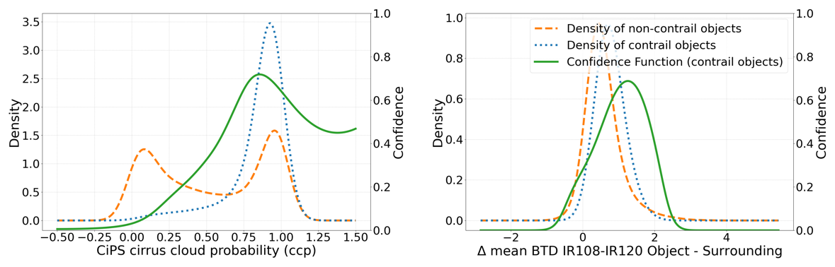
Figure 4 Example of probability densities of values of non-contrail objects (orange, dashed) and contrail objects (blue, dotted) in the training dataset, non-contrail objects being objects that appear in the binary mask derived by adaptive thresholding but not in the ground truth of the training dataset and contrail objects being objects that appear in both, and derived confidence functions (green, solid), defined as the fraction of contrail objects in the total density of objects at that value, for the CiPS cirrus cloud probability (ccp) and the difference of the mean BTD IR108-IR120 between objects and surrounding area.

3.4 Linear Object Separation

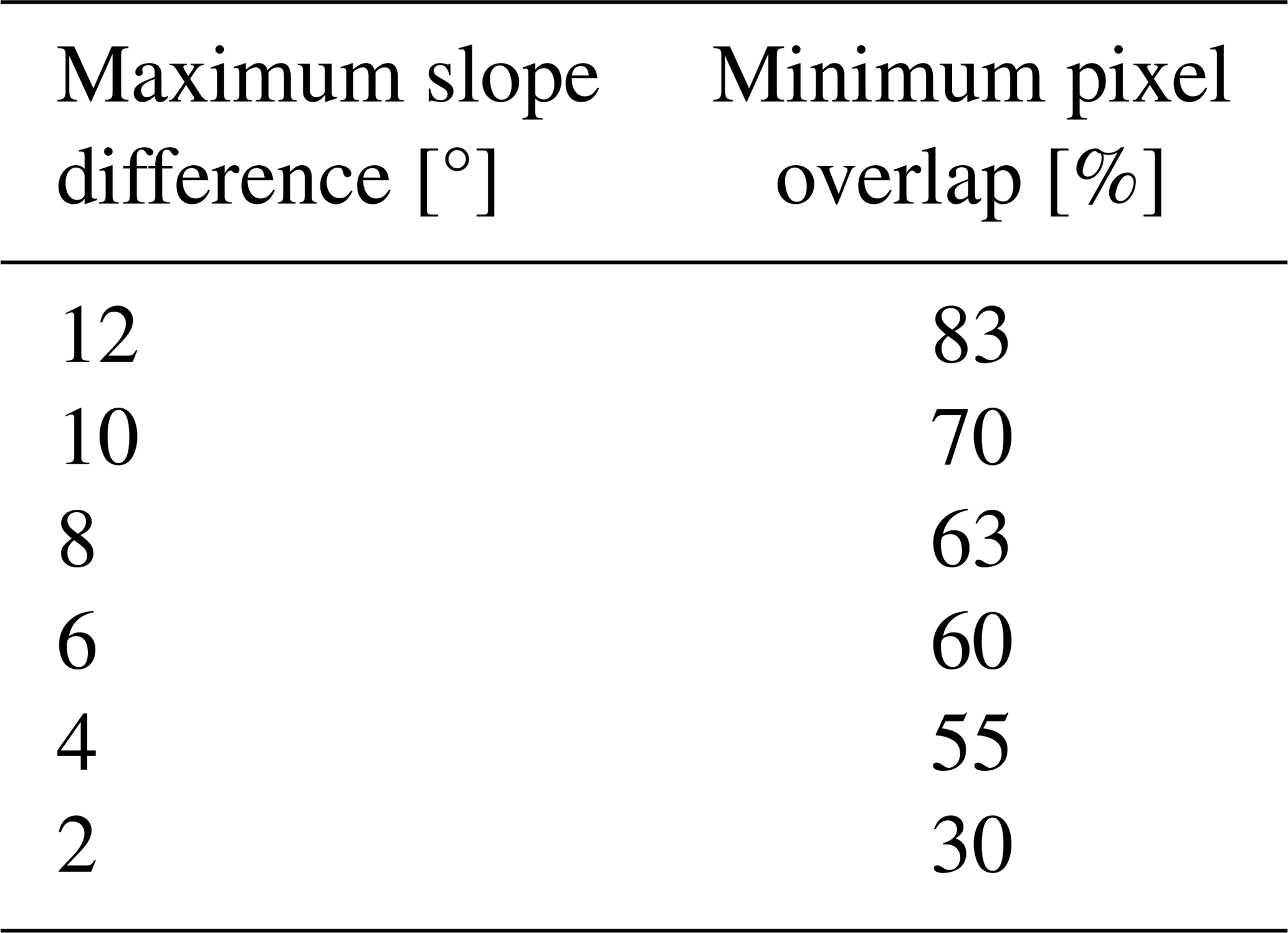
In order to separate contrails from false alarms in the adaptive thresholding mask AT, we not only ensure that the single retrieved pixels satisfy given conditions, but we also consider contiguous pixels as objects and evaluate their characteristics (see following section). In fact, linearity has not been required yet for the pixels/objects to represent contrails. We describe the method for linear object separation in the following. At this stage we identify each line-shaped pixel batch as a separate object. This can be difficult starting from the binary image AT produced above in Sect. 3.2, especially if multiple contrails intersect. In the first step, connected objects are isolated using the 8-connection criterion. The 8-connection criterion defines pixels as connected if they touch each other along edges or corners, considering all eight neighboring positions in a 2D grid. If the number of pixels of those connected objects does not exceed five, then the objects are discarded. This removes the majority of the small patches in Fig. 3b. In the next step, we investigate the linearity of the objects. A line detection is performed using the probabilistic Hough Line Detection (PHL, see Appendix B). If no line can be found in a connected object, it is discarded. If only one line can be found, then the object is retained as one linear object. If the PHL finds multiple lines in an object, it has to be divided into linear sub-sets. To do this, pixels are assigned to each PHL line. Pixels that are connected in the binary AT image produced by adaptive thresholding and have a Euclidean distance of less than 1.5 pixels from the line obtained by the PHL are assigned to that line (wider objects have multiple PHL lines that are later merged together, so this assignment does not affect properties of the whole object). This distance is selected in agreement with the typical width of 10–15 km found in Vázquez-Navarro et al. (2015). This distance is selected as we focus mainly on detecting linear contrails and want to avoid assigning pixels of another intersecting contrail. Pixels that are too far away from any detected PHL line are discarded. Objects consisting of pixels assigned to each PHL line are referred to as “PHL objects”. As (especially older) contrails might be wide line-shaped objects and not thin lines, the PHL might find multiple lines with similar slopes in a single line-shaped object. Detected lines that belong to the same linear object and have similar slopes are merged together. In order to implement this, not only the slope of each PHL object is calculated but also the amount of overlapping pixels to another PHL object. An empirically defined set of tolerance pairs (Table 2) of maximum slope difference s_max and minimum fraction of pixels that overlap in the two PHL objects o_min (the fraction is computed w.r.t. the smaller PHL object) is used to merge PHL objects: they are merged (all pixels of both PHL object are considered as one object) if their slopes differ by at most s_max and their number of overlapping pixels is larger or equal than o_min. This is done for all connected components in the binary image AT that is produced by adaptive thresholding. Using this method, we obtain all line-shaped objects as separate outputs (Fig. 3c). This method can separate individual line shaped objects well, but has difficulties if two individual lines are touching and have a very similar slope.

Table 2 Tolerance pairs for maximum slope difference and minimum overlap (overlapping number of pixels compared to number of pixels of smaller line) for two lines obtained from PHL to be merged together. Tolerance pairs were set based on empirical evaluation, selecting the values that yielded the most effective outcome.

After application of this linear object separation, the results of the thresholding contained in the AT mask can be further investigated in two ways in order to reduce false alarms: pixel-wise and object-wise.

3.5 Evaluation Procedure

The binary mask AT is subjected to three parallel evaluations to determine the likelihood of contrail presence. For each line-shaped object, two different tests are performed to assess whether they are likely to be contrails or not. In parallel, a pixel-wise test is performed. These evaluation steps are described in the following sections.

3.5.1 Pixel-wise Check

The pixel-wise tests are described in this paragraph. Pixels that appear bright in the input image and are returned by the adaptive thresholding need to be evaluated to determine if they are indeed contrail pixels. The following pixel-wise properties are tested:

1. Ice cloud properties (cirrus cloud probability, cirrus opacity probability, cloud top height, ice optical thickness, ice water path, ice crystal effective radius) derived from CiPS (Sect. 2.2) are used for this pixel-wise evaluation.

2. In line with Mannstein et al. (1999), the large scale maximum gradient of the IR120 brightness temperature is used (see Sect. 2.3 for a detailed explanation).

3. The BTD between IR108 and IR120 is used, as it is known to have larger values for contrail pixels.

4. Additionally, the BTD WV062 – WV073 between the two water vapor channels WV062 and WV073 and the BT IR039 are used.

For all of the above mentioned parameters, the contrail confidences are looked up from the pre-computed confidence functions (see Sect. 3.3). The mean of these confidences is used as contrail confidence score S_pe for every pixel. Pixels with zero mean contrail confidence are removed. Based on this set of pixel scores, a recombination (see Appendix C) is performed at the end of this step to close holes in objects that the pixel-wise evaluation might have caused by assigning a contrail confidence of 0. This recombination only affects pixels that were included in the binary mask AT, it does not close holes that were already present in AT. This is done to not alter the morphology of the detected objects.

3.5.2 Object-wise Check: Morphological Tests

For each line-shaped object, a set of morphological properties is used to determine its likelihood to be a contrail. The length, mean width, maximum width, standard deviation of widths and number of holes are calculated for every contrail candidate. All of the above mentioned morphological properties are then evaluated by assigning a confidence score based on the confidence function (see Sect. 3.3) for each property. The final confidence score of a contrail candidate for this morphological check S_me is determined as the mean value of all individual morphological scores.

3.5.3 Object-wise Check: BTD Tests

In this part of COCOS, four BTDs, namely IR087 – IR108, IR039 – WV062, IR108 – IR120 and WV062 – WV073, are used to evaluate contrail likelihood. Two of those BTDs were already previously used for the creation of the input image (Sect. 3.1), but are being used here as mean object-wise values. Although IR039 comprises both solar and thermal components, we do not apply a day–night separation. This choice is motivated by the fact that our algorithm relies on relative contrast, for which the combined signal remains informative regardless of illumination conditions. The mean BTD of the object is subtracted from the mean BTD of the immediate surrounding of the object (see Sect. 3.3). As for the pixel-wise check and the morphological check, contrail confidences are looked up from the pre-computed confidence functions for the four BTDs. The mean over these four confidences for each object is the contrail confidence score S_oe, analogous to the other two checks.

3.6 Contrail Confidence Score

At this stage, we have obtained the binary mask AT by performing adaptive thresholding on an input image. Through the linear object separation we have discarded small and/or non-linear objects. The pixel-wise check, the object-wise morphological check and the object-wise BTD check have each provided contrail confidence scores (S_pe, S_me and S_oe) for the remaining pixels/objects. We now combine these quantities pixel-wise to obtain the final confidence score for the contrail pixels. A penalized mean is used to produce the final output of COCOS (Fig. 3d) using the three confidence scores given above. The penalized mean is calculated as

$$\begin{array}{}\text{(3)}& \begin{array}{rl}& {\mathrm{mean}}_{\mathrm{penalized}}(S_{\mathrm{pe}},S_{\mathrm{me}},S_{\mathrm{oe}})\\ & ={\displaystyle \frac{\mathrm{1.1}\times \mathrm{mean}(S_{\mathrm{pe}},S_{\mathrm{me}},S_{\mathrm{oe}})\times \min (S_{\mathrm{pe}},S_{\mathrm{me}},S_{\mathrm{oe}})}{\mathrm{0.1}+\min (S_{\mathrm{pe}},S_{\mathrm{me}},S_{\mathrm{oe}})}},\end{array}\end{array}$$

where mean is the arithmetic mean of the three confidence levels and min is the lowest confidence score. This method to calculate the final confidence weighs low values more than high values. If one of the property groups gives a low score of an object being a contrail, this drastically reduces its final confidence score because we expect contrails to provide high confidence scores in all three aspects. To provide a contrail mask as in previous work by Mannstein et al. (1999) or Dekoutsidis et al. (2023), a threshold for the confidence score must be selected (see discussion below). The contrails can then be saved in the geojson file format as line segments and/or multi-point objects. Comparing the Ash RGB in Fig. 1 and the corresponding final confidence score in Fig. 3d, one can see that most objects within the natural ice cloud on the upper left show low confidence scores, generally lower than 0.4. The two dark objects in the Ash RGB have confidence scores around 0.20, despite linearity. Contrails are characterized by moderately high confidence scores up to 0.60. Most of them have relatively uniform confidence scores, with only small portions of them showing lower values (reddish colors, confidence score around 0.40).

4 Detection Results and Analysis

In this section we evaluate the performance of COCOS using the 89 contrail images from the evaluation dataset (see Sect. 2.4).

4.1 Precision and Recall

The contrail detection returns a contrail confidence score for each pixel. The contrail confidence score should not be interpreted as a true probability – for example, a score of 0.6 does not imply 60 % certainty – but rather as a relative measure, with higher scores indicating greater confidence that a detected feature is a contrail. The user can then set a threshold to create a binary contrail mask, based on the desired application of the output. An example of contrail masks using different confidence thresholds is shown in Fig. 5. One can see that increasing the threshold from 0.45 to 0.50 to 0.55 reduces the amount of contrails detected. Depending on the confidence threshold, the result has thus different capabilities. It always comes with a trade-off between a high detection efficiency and a low false alarm rate.

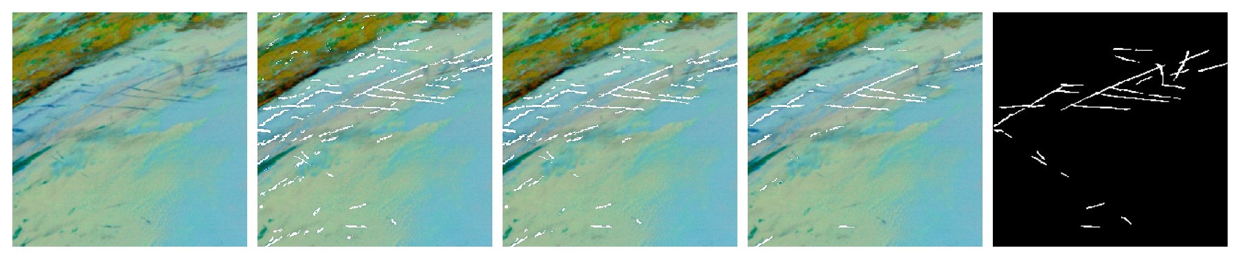
Figure 5 The leftmost panel shows an Ash RGB image with several contrails. The three panels to the right display detection results using confidence thresholds of 0.45, 0.50, and 0.55, respectively. The rightmost panel shows the ground truth that was determined by the majority agreement of three labelers.

The precision-recall trade-off is investigated in detail in the following and COCOS is also compared to Mannstein's versions (see Sect. 2.3). By applying different confidence thresholds to the output of COCOS, a performance curve can be obtained showing recall and precision for different thresholds (for a detailed explanation of the evaluation metrics see Appendix A). Due to the distribution of confidence scores across the images in the evaluation dataset (Fig. 6), the authors suggest that confidence scores below 0.4 or above 0.6 are not meaningful to produce binary contrail masks. A confidence threshold of 0.465 maximizes the difference between correctly detected positives and incorrectly detected negatives. Figure 7 shows a performance curve using confidence thresholds ranging from 0.35 to 0.65 in increments of 0.025, with calculation of precision and recall being performed on a pixel-wise and contrail-wise level (see Appendix A1 for calculated values). For the object-wise determination of the performance parameters, we only count a contrail as successfully detected if at least half of it is detected.

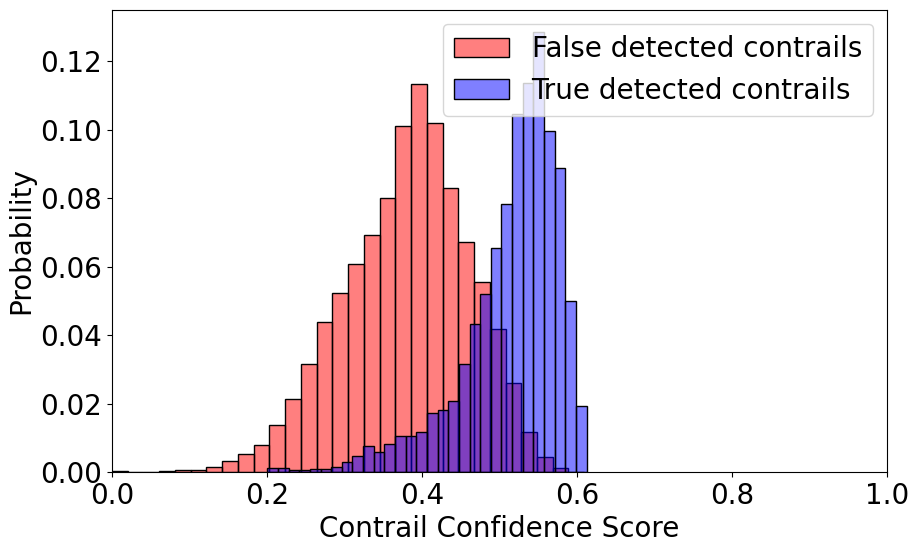
Figure 6 Distribution of contrail confidence scores from COCOS applied to the evaluation dataset separated in true (blue) and false (red) detections as determined by comparison with the human-labeled reference data.

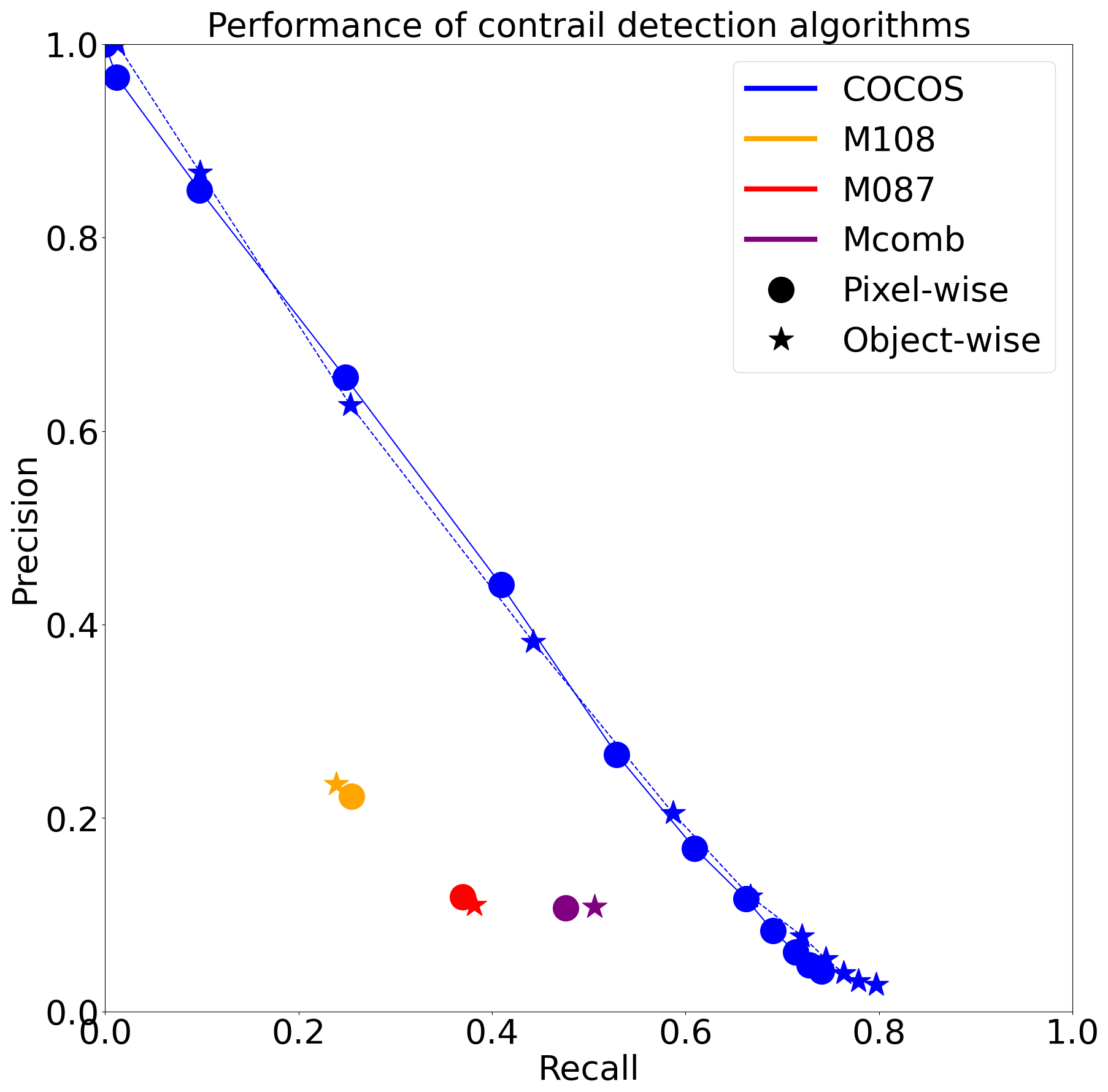
Figure 7 Per-contrail and per-pixel precision-recall curve for COCOS at confidence thresholds ranging from 0.35 to 0.65 in increments of 0.025, compared with the precision and recall of other contrail detection algorithms (adaptations of Mannstein et al., 1999) applied to MSG data.

Of course, a higher confidence threshold leads to higher precision at the cost of lower recall. Using a confidence threshold of 0.45 produces a pixel-wise recall of 66 % and precision of 12 %, while using a confidence threshold of 0.55 leads to a pixel-wise recall of 25 % and precision of 65 %. For lower confidence thresholds, the object-wise recall is always higher than the pixel-wise and precision is lower. This suggests that contrails are detected, but only in part, leaving some pixels undetected and few additional pixels (that do not appear in the ground truth) are detected in each detected contrail. Misdetected objects seem to have a low number of pixels. This behavior reverses at high confidence thresholds, where less than a third of contrails from the ground truth are found in COCOS. Here, the algorithm is stricter and the previously at least partially detected contrails are lost. Even with the lowest confidence thresholds no more than 80 % of contrails are detected by COCOS. Non-detectable contrails exhibit a notably shorter average length of 13.58 pixels compared to 27.94 pixels observed in detected contrails. Moreover, surrounding and underlying cloud types associated with non-detectable contrails more frequently correspond to Thin Ice, Thick Ice, and Supercooled Liquid phases compared to detected contrails. Specifically, Thin Ice accounts for 50.3 % of the cloud types around non-detectable contrails, compared to 40.8 % for detected contrails. Similarly, Thick Ice is present in 1.5 % of non-detectable contrails versus 0.54 % in detected contrails, and Supercooled Liquid accounts for 0.5 % of non-detectable contrails compared to 0.27 % in detected contrails. These percentages represent the proportion of each cloud type relative to the total cloud types observed for detected and non-detected contrails, respectively. Additionally, the proportion of land surface beneath non-detectable contrails is slightly higher relative to that of detected contrails. 30 % of non-detected contrails are over land, while only 20 % of detected contrails are over land.

4.2 Comparison to existing methods

In order to assess the performance of COCOS against comparable results for the same satellite and the same dataset, we have used three contrail detections from the literature (shortly described already in Sect. 2.3). Their performance is also illustrated in Fig. 6. M108 has the higher precision of the three (around 0.22), but the smallest recall (around 0.25). M087 and Mcomb have higher recall (above 0.45 for Mcomb), but even smaller precision (0.11). COCOS outperforms all of the other three algorithms. At the same recall levels, it achieves precision values that are up more than three times higher (0.65 for recall 0.25 and 0.3 for recall 0.5). It also offers the advantage of multiple precision/recall pairs depending on the chosen confidence threshold. The other algorithms only return one binary mask and perform at fixed precision and recall values. For a balanced precision-recall trade-off without favoring either metric, the recommended default confidence threshold for COCOS is 0.465. One can also view these results in the broader context of recent AI-based contrail detection algorithms developed for GOES. Meijer et al. (2022) reported a pixel-wise precision of 52.5 % and recall of 50.2 % using convolutional neural networks (CNNs), while Ng et al. (2024) achieved 80 % precision at a similar recall using a multi-frame CNN model. At comparable recall levels (around 50 %), COCOS reaches a precision of 35 %. However, these numbers are not directly comparable: the studies differ in satellite sensor characteristics, spatial resolution, observational domain, time period, input data, and evaluation criteria. Indeed, skill scores are known to transfer poorly between independent studies. What can reasonably be stated is that other AI-based work for geostationary satellites of the current generation (with better spatial resolution than MSG/SEVIRI) has reported similar, though generally higher, skill, which may result from differences in data, methods, evaluation approaches, or a combination thereof.

4.3 Dependency of Performance on background and contrail properties

We now turn to a detailed analysis of the algorithm performance across various contrail and background properties to better understand the factors influencing its effectiveness. As the dataset is spatially non-uniform, we refrain from comparing performance across regions. In the following, performance curves are generated for different linearity values, surface types, underlying clouds and ice optical thicknesses of contrails in the evaluation dataset. As shown in Fig. 8, the performance curves illustrated for linearity, surface types and ice optical thicknesses in Fig. 9 can be reliably interpreted, as the number of examples in each category is sufficiently large to be representative (over 50 contrails, with a total number of contrails in the evaluation dataset of 651). In the evaluation dataset there are very few contrails over mixed-phase, supercooled liquid or thick ice clouds as these cloud top phases are observed very rarely in the dataset overall. Thus these performance curves are more uncertain.

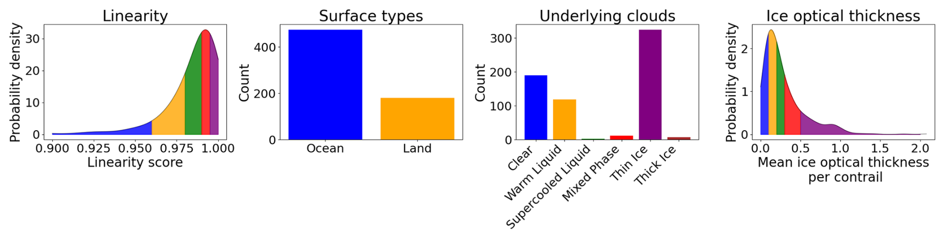
Figure 8 Distributions of 651 contrails in the human-labeled evaluation dataset across multiple categories in linearity, surface types, underlying clouds and ice optical thickness.

The performance of COCOS shows a clear positive correlation with increasing contrail linearity (as defined in Sect. 3.5.2), as illustrated in Fig. 9a. In fact, there is a strong increase in precision and recall when linearity is larger than 0.995. For these contrails, a recall of 0.7 can be achieved with a precision larger than 0.9. This outcome is expected and aligns well with the primary objective of COCOS, which is specifically designed to identify thin, elongated structures such as contrails. Young contrails that maintain a well-defined linear shape – likely observed 90 min after aircraft passage (Gierens and Vázquez-Navarro, 2018) – can be more readily distinguished from natural cirrus or other cloud types. These structures have grown large enough to be visible in SEVIRI observations, but are also young enough to preserve their linear shape and exhibit strong geometric contrast and are less likely to blend into the background cloud field, making them ideal targets for linear-feature-based detection techniques.

The analysis further reveals differences in algorithm performance related to the background, with slightly better results over oceanic regions compared to land surfaces (Fig. 9b). Several factors may contribute to this disparity. Over the ocean, the thermal and radiative background is generally more homogeneous, which can enhance the contrast between contrails and the underlying surface. Land surfaces, in contrast, often exhibit greater heterogeneity due to variations in topography, vegetation, and temperature, potentially introducing more noise and confounding features that interfere with reliable detection (see, e.g., the discussion in  Mannstein et al., 1999).

Cloud conditions also play a significant role in detection success. As shown in Fig. 9c, COCOS performs best under clear-sky conditions or when contrails are located above low, warm liquid clouds. These scenarios typically provide strong thermal radiative contrast between the contrail and the background, improving detection confidence. In contrast, the presence of thin ice clouds below the contrail introduces a greater challenge. These cloud types can exhibit similar spectral and spatial characteristics to contrails, making separation more difficult. The data basis for detection over thick ice clouds is too limited to draw reliable conclusions; however we assume that the detection challenge becomes even more pronounced over thick ice clouds, where the dense cloud layer below often masks the presence of any overlying contrails. In such conditions, confident detection becomes nearly impossible due to the lack of contrast. This challenge becomes evident when visually inspecting and labeling satellite images and might be the reason for the low amount of contrails labeled over thick ice clouds.

The limited detection efficiency over thick ice clouds is confirmed when we look at the ice optical thickness (Fig. 9d). Ice clouds with high optical thickness tend to obscure the contrail signal, reducing visibility in the satellite imagery and making accurate identification more difficult. Conversely, when the underlying ice clouds are optically thinner, the radiative signature of the contrail remains more pronounced, and COCOS performs significantly better. It should be noted that the optical thickness values reflect the combined signal of the contrail and the underlying cloud, as the satellite cannot differentiate between them when the contrail lies on top of an ice cloud. This aligns with Driver et al. (2025), who find that detections for a SEVIRI-resolution imager are only possible for ice optical thicknesses around 0.1 (assuming a clear-sky background). This sensitivity to optical depth underscores the importance of accurately characterizing the surrounding cloud environment when applying the algorithm.

Taken together, these findings emphasize that the performance of COCOS is not uniform across all environmental conditions. Instead, it varies with factors such as contrail morphology, surface type, underlying cloud phase, and (ice cloud) optical depth. Understanding these dependencies is crucial not only for interpreting detection results but also for users to assess how COCOS behaves in specific situations and to interpret the results more effectively.

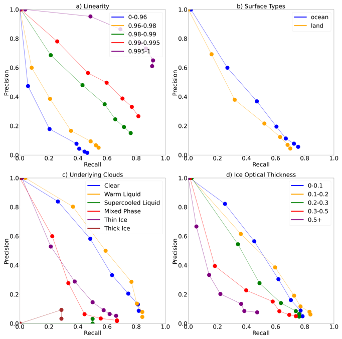
Figure 9 Per-contrail precision/recall curves with lines grouped by (a) contrail linearity, (b) surface type, (c) cloud-top phase of underlying clouds and (d) ice optical thickness. Each line represents a different category, showing how detection performance varies across these groups.

4.4 Contribution of individual evaluation steps

Beyond analyzing external factors like background and contrail properties, we are also investigating the “why” behind our algorithm's success. We want to determine which evaluation steps of our pipeline are the primary drivers of accurate detection. Gaining this granular understanding will be a major asset as it will provide critical guidance for the development of improved contrail detection methodologies. For this investigation the algorithm was deployed multiple times with individual evaluation steps excluded. The investigated versions of the algorithm include the following:

1. Neglecting any CiPS outputs

2. Not checking the morphological properties of the objects

3. Omitting the object-wise BTD test

4. Excluding the pixel-wise properties apart from CiPS outputs

5. Leaving out any pixel-wise properties

The performance curves for these versions compared to the normal COCOS version can be seen in Fig. 10. This ablation analysis of the detection pipeline reveals that the morphological evaluation is the most critical determinant of model precision. When this step is omitted, the algorithm fails to surpass a 20 % precision threshold, suggesting that geometric constraints are indispensable for filtering non-contrail artifacts. The second most significant contribution stems from the pixel-wise verification step. Within this step, a hierarchy of influence is observed: the exclusion of the thermal gradient and Brightness Temperature Differences (BTD) resulted in a more pronounced performance decay compared to the exclusion of CiPS outputs alone. This suggests that low-level radiometric features, such as BTD and gradients, offer a more stable foundation for detection than high-level derived products like CiPS. Finally, while the object-wise BTD check was found to have the least relative impact on “worsification”, its removal still led to a substantial degradation in performance, confirming its necessity as a final refinement step in the detection algorithm.

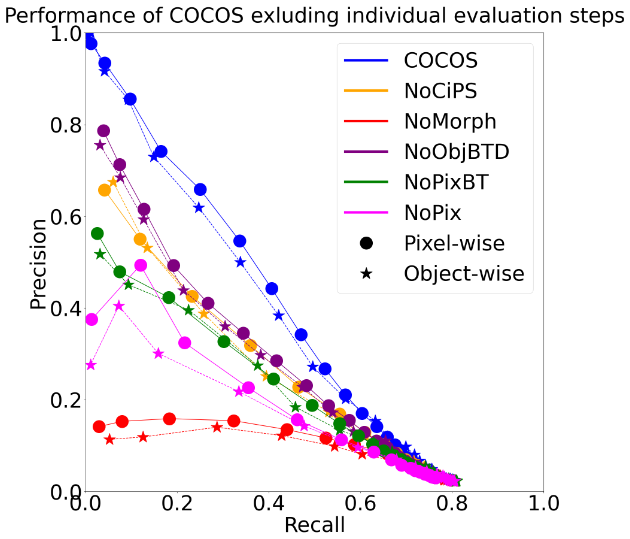
Figure 10 Per-contrail and per-pixel precision-recall curve for COCOS with all its evaluation steps compared to the algorithm with individual evaluation steps excluded. The investigations include: NoCiPS – without the usage of any CiPS outputs, NoMorph – not checking the morphological properties of the objects, NoObjBTD – not calculating the object-wise BTD, NoPixBT – not checking the pixel-wise properties apart from CiPS outputs, NoPix – not using any pixel-wise properties.

5 Conclusions

This study presents a novel contrail detection algorithm named COCOS tailored to the SEVIRI instrument aboard the Meteosat Second Generation (MSG) satellite. COCOS demonstrates superior performance over existing approaches for MSG, achieving significantly higher precision and recall in various test scenarios. At comparable recall levels, it attains more than three times the precision of previously established methods for MSG/SEVIRI (0.65 for recall 0.25 and 0.3 for recall 0.5), highlighting its robustness and reliability in detecting linear contrail features. The success of this approach lies in several methodological advancements. Notably, the implementation of adaptive thresholding allows for a dynamic response to changing image characteristics such as brightness gradients and background cloud variability. Additionally, the sophisticated line detection and separation and analysis of linear structures enhance the algorithm’s ability to distinguish contrails from other cloud formations and artifacts. Importantly, COCOS does not merely produce a binary mask indicating contrail presence; it also assigns a confidence score to each detected structure, thereby providing users with a quantifiable measure of precision recall trade-off. By choosing a variable confidence threshold, the algorithm is suitable for a range of different applications where either high detection rate or low false alarm rate might have a higher importance. While COCOS performs well compared to other detection algorithms for SEVIRI, the limited spatial resolution still makes confident contrail identification challenging. In particular false alarms remain high in many scenarios. In addition, the scarcity of reliable ground truth further complicates the evaluation and validation of detection performance, since even manually labeled contrails are subject to large uncertainties due to the same reasons. In the future, high-resolution lidar data from the EarthCARE mission may prove helpful in addressing these gaps, providing the precise vertical profiling necessary to quantify the detection accuracy and physical characteristics of these features with far greater certainty.

In terms of further development of the method, COCOS can be extended to other satellites with only a few modifications – by using for instance the spectral-band adjustment factors proposed by Piontek et al. (2023) – since similar channels to those used for COCOS are available in most currently operational polar- and geostationary-satellite passive imagers, incorporating additional channels, or making small algorithmic adaptations. However, the method’s performance is fundamentally constrained by the quality of human labels. The Flexible Combined Imager (FCI) aboard the satellite following on from MSG (Meteosat Third Generation – MTG, launched on 13 December 2022; Durand et al., 2015) has additional channels in the near infrared which can improve contrail detection and can be easily included in the workflow of COCOS. Future work will focus on extending the approach to MTG/FCI data to benefit from the higher spatial and temporal resolution as well as the additional channels. This extension of the algorithm is essential to ensure reliable contrail detection over Europe, as MSG and MTG are the only geostationary satellites providing continuous coverage of this region with dense air traffic. Beyond detection, this algorithm has potential applications in assessing the spatial and temporal distribution of contrails, evaluating the effectiveness of mitigation strategies (such as flight rerouting), and improving the representation of aviation-induced clouds in climate models and contrail models. By providing a tool that is both accurate and adaptable, this work contributes meaningfully to ongoing efforts in understanding, monitoring and reducing the climate impact of aviation-induced cirrus.

Appendix A: Evaluation metrics

The choice of evaluation metric for contrail detection should align with the intended application. If the focus is on estimating the radiative forcing of contrails, a per-pixel metric is appropriate, as it reflects the total area affected. On the other hand, when the goal is to link contrails to specific flights or to measure their lengths, per-contrail metrics provide more relevant insights. In this work, we consider both types of metrics to provide a comprehensive assessment of contrail detection performance. Different applications may require different contrail confidences with more focus on high detection rate or more focus on little false alarms. Therefore, single-value metrics such as Intersection over Union (IoU; Rezatofighi et al., 2019) or the DICE (Dice, 1945) coefficient are not investigated in detail in this work, but we provide the DICE coefficient in the following for easier performance comparison. Instead, we focus on both precision and recall, as they offer a more informative view of detection performance by quantifying how many contrails are correctly identified and how many false detections occur. Precision measures the fraction of detected contrail pixels or contrails that are actually true contrails, indicating how reliable the detections are compared to an established ground truth. Recall, on the other hand, measures the fraction of true contrail pixels or contrails that are successfully detected, reflecting how completely the method captures contrail occurrences. Together, these metrics provide a balanced view of detection quality, highlighting both false positives and missed detections. Let TP denote the number of true positives (correctly detected contrail pixels or objects), FP the number of false positives (non-contrail pixels or objects incorrectly detected as contrails), and FN the number of false negatives (missed contrails). Then, precision and recall are defined as:

$$\begin{array}{}\text{(A1)}& \mathrm{Precision}={\displaystyle \frac{\mathrm{TP}}{\mathrm{TP}+\mathrm{FP}}},\mathrm{Recall}={\displaystyle \frac{\mathrm{TP}}{\mathrm{TP}+\mathrm{FN}}}\end{array}$$

A1 COCOS Performance

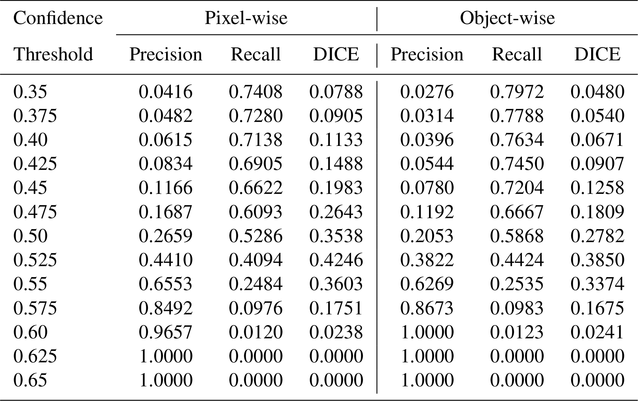
We provide a detailed table showing object-wise and pixel-wise precision, recall and DICE score for binary contrail masks generated by using confidence thresholds between 0.35 and 0.65 (see Table A1).

Table A1 Object-wise and pixel-wise precision and recall for varying confidence thresholds used to generate a binary contrail mask from COCOS output

Appendix B: Hough Line Detection

To detect line segments in an image, the Probabilistic Hough Transform (PHT) is used (Matas et al., 2000). Unlike the standard Hough Transform, PHT returns line segments defined by their endpoints. Each line is represented in polar coordinates (ρ,θ), where ρ is the perpendicular distance to the origin and θ is the angle of the normal vector with respect to the x-axis.

$$\begin{array}{}\text{(B1)}& \mathit{\rho }=x\cos \left(\mathit{\theta }\right)+y\sin \left(\mathit{\theta }\right)\end{array}$$

The algorithm uses a 2D accumulator array over ρ and θ, where each edge pixel casts votes for all lines passing through it. Peaks in the accumulator correspond to likely line candidates. To reduce computational cost, PHT randomly samples a subset of edge pixels. Once candidate lines are identified, the algorithm traces along the line direction to determine the endpoints of the segment, taking into account a user-defined minimum segment length and maximum allowed gap between pixels. We use 5 pixels as the minimum segment length and 2 pixels as the maximum gap allowed.

Appendix C: Recombination

To close holes in a line-shaped object that a pixel-wise evaluation of conditions might have caused (Sect. 3.5.1), a recombination strategy is needed. First a binary dilation is performed to add a one-pixel thick border around each pixel in the binary mask. The neighborhood sum of this dilated image is then calculated by convolving it with a kernel of size 3 × 3. A pixel is filled in the original image if this neighborhood sum is greater than 8, meaning that all surrounding pixels are filled in the dilated image. This method can close holes of up to 2 pixels thickness (Fig. C1). This method closes holes resulting from the pixel-wise evaluation of contrail conditions, without filling any pixels that were not already set to 1 in the binary mask AT before applying the pixel-wise evaluation.

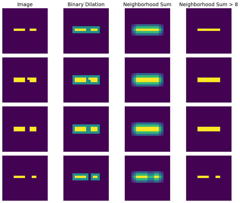
Figure C1 Illustration of recombination strategy to close gaps and holes in objects. Four different starting situations are shown in the leftmost column together with the steps described in the text.