Bayesian denoising of satellite images using co-registered NO₂ images

Accurate emission tracking (e.g., locating and quantifying hot spots) using satellite images requires a good signal-to-noise ratio (SNR) of total column images. Achieving this SNR is challenging for satellite-based trace gas imagers, especially when enhancements are small relative to the background or small relative to retrieval uncertainty. Therefore, some satellites carry additional trace gas imagers with high SNR, such as NO₂, which is co-emitted with the trace gas of interest. While NO₂ is frequently used qualitatively for plume detection or plume fitting, its potential for quantitative noise reduction remains largely untapped. This paper presents two methods to enhance the SNR of total column images using co-registered NO₂ images through minimum mean square error (MMSE) Bayesian denoising, which are a simple form of a Kalman filter or maximum a posteriori estimate. The first “joint MMSE” method relies on the presence of plumes in both the low- and co-registered high-SNR NO₂ images. The second “self-similar MMSE” method utilizes image self-similarity and is based on an existing technique called BM3D. The methods are evaluated using a synthetic dataset (SMARTCARB) of atmospheric CO₂ and NO₂ concentrations, achieving over +40 dB improvement in peak SNR (i.e., an over 10${}^{(\mathrm{40}/\mathrm{10})}$ increase in SNR). Additionally, the methods are applied to TROPOMI SO₂ and NO₂ data over South Africa and used to compute a divergence image, demonstrating that an estimated 40 %–80 % noise reduction is possible. By enhancing the SNR of total column images, these techniques improve the detectability of subtle emission signals, which could benefit atmospheric monitoring applications.

1 Introduction

To quantify emissions and support climate policy, satellite-based monitoring system are developed that will detect and quantify emissions plumes from cities and large point sources (hereafter referred to as “hot spots”). To perform emission quantification for hot spots, a good signal-to-noise ratio (SNR) is essential; first to be able to detect the plumes, and second to be able to quantify the plume enhancements with good accuracy. Achieving this for satellite observations of CO₂ is challenging, as enhancements (∼ 0–5 ppm) are minor compared to background levels (∼ 420 ppm) and retrieval uncertainties are high (Miller et al., 2007). Therefore, CO₂ monitoring satellites like the Global Observing Satellite for Greenhouse gases and Water cycle (GOSAT-GW), the Copernicus Anthropogenic Carbon Dioxide Monitoring (CO2M) mission and the Twin Anthropogenic Greenhouse Gas Observers (TANGO) mission will carry an additional NO₂ instrument. NO₂ is useful because it is co-emitted with CO₂ during high-temperature combustion while it can be measured with a much better SNR. NO₂ thus helps delineating and thereby quantifying the low SNR CO₂ plumes using emission quantification methods. So far, approaches in the literature have used the information contained in the NO₂ observations mainly qualitatively. For example, they guided plume detection or constrained a Gaussian curve fitted to plume transects (Reuter et al., 2019; Kuhlmann et al., 2019, 2021). One prominent emission quantification method, the divergence method (Beirle et al., 2019, 2023; Koene et al., 2024), cannot effectively leverage the superior SNR of the co-registered NO₂ data, as it does not depend on plume detection. As the divergence method is highly susceptible to noise in the data due to its derivative operations, Hakkarainen et al. (2022) proposed to apply a mean filter to prepare the noisy CO2M CO₂ images for the divergence method; however, such spatial smoothing risks blurring emission signals at the source.

In this paper, we explore two data-driven methods to enhance the SNR of trace gas images using the co-registered NO₂ images (a process also referred to as “denoising”). Compared to alternatives like a model-driven denoising approach relying on meteorological, emission, and satellite noise priors, a data-driven method requires fewer assumptions, as the empirical cross-field covariance between co-registered images is learned directly from the data. An example of the proposed methods is given in Fig. 1, which illustrates the effectiveness in reducing noise in a SO₂ image recorded by the TROPOspheric Monitoring Instrument (TROPOMI; Veefkind et al., 2012). The two methods are minimum mean square estimators (MMSEs). The first is based on the joint information in CO₂ and NO₂ pixels. The second is based on image self-similarity. Put simply, the MMSEs we present are operations that extract a denoised signal from two (or more) noisy inputs in a Bayesian optimal way, much like a Kalman filter. We define the estimators in the theory section, and suggest to chain them in series to provide the best results. Within the results section of the paper, we verify the method by applying it to synthetic CO2M data to denoise synthetic CO₂ images. We then show a “real data” example using combined TROPOMI SO₂ and NO₂ data and use the denoised SO₂ data to denoise the corresponding divergence map.

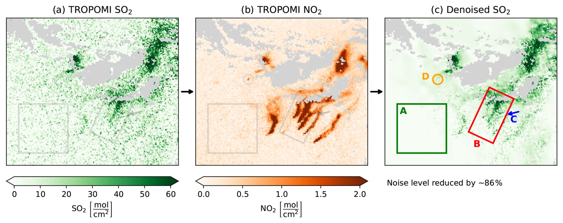
Figure 1 Example of the denoising procedure for a South African region, recorded by TROPOMI on 20 February 2021. Axis labels are omitted to emphasize the clarity of the denoised image rather than geographical location. Data with a quality factor below 0.75 is masked and appears as plain gray. By optimally combining the (a) “noisy” SO₂ and (b) less “noisy” NO₂ images, we create a (c) denoised SO₂ image. We highlight some features of the denoised image. Square A shows that in areas without signal, noise is effectively removed from the image. Rectangle B indicates that plume signals present in the noisy data are retained, resulting in an enhanced signal-to-noise ratio. Arrow C illustrates an east-west (i.e., right-left) feature with low amplitude but sharp, high contrast edges, identifiable in the original SO₂ image but absent in the NO₂ image, confirming that significant “positive” and “negative” signals are preserved during denoising. Circle D shows a feature of high amplitude in the NO₂ image which is absent in the SO₂ image, indicating we do not add signal unduly. The noise level estimate is derived from Immerkaer (1996).

2 Methods

The two denoising methods presented in the following will be referred to as the “joint MMSE” approach and the “self-similar MMSE” approaches. The former is a novel innovation, whereas the latter is a pre-existing method from the field of computer vision, which we adapt for denoising co-registered images.

2.1 Joint MMSE (jMMSE)

In this section, we explore a method that makes use of the joint information in two co-registered signals at the pixel level. The theory may alternatively be derived from a Bayesian inference point of view, as shown in Sect. S1 in the Supplement.

2.1.1 Observation model

Satellite data of two co-registered pixels of, say, CO₂ and NO₂ follow a general model like

$$\begin{array}{}\text{(1)}& \left[\begin{array}{c}{\stackrel{\mathrm{̃}}{\text{CO}}}_{\mathrm{2}}\\ {\stackrel{\mathrm{̃}}{\text{NO}}}_{\mathrm{2}}\end{array}\right]=\left[\begin{array}{c}{\text{CO}}_{\mathrm{2}}\\ {\text{NO}}_{\mathrm{2}}\end{array}\right]+\left[\begin{array}{c}{n}_{{\text{CO}}_{\mathrm{2}}}\\ n_{{\text{NO}}_{\mathrm{2}}}\end{array}\right],\end{array}$$

where the tildes indicate noisy observations; CO₂ and NO₂ denote the noise-free but unknown true values, and $n_{{\text{CO}}_{\mathrm{2}}}$ and $n_{{\text{NO}}_{\mathrm{2}}}$ indicate the noise on the measurements. We can rewrite this model into a coupled observational model by making it a function of the noise-free CO₂ data,

$$\begin{array}{}\text{(2)}& \begin{array}{rl}\left[\begin{array}{c}{\stackrel{\mathrm{̃}}{\text{CO}}}_{\mathrm{2}}\\ {\stackrel{\mathrm{̃}}{\text{NO}}}_{\mathrm{2}}\end{array}\right]& =\left[\begin{array}{c}\mathrm{1}\\ d(x,y)\end{array}\right]{\text{CO}}_{\mathrm{2}}+\left[\begin{array}{c}{n}_{{\text{CO}}_{\mathrm{2}}}\\ n_{{\text{NO}}_{\mathrm{2}}}\end{array}\right]\\ & =\stackrel{\mathrm{̃}}{\mathit{M}}=\mathit{H}c+\mathit{n}\end{array}\end{array}$$

where $\stackrel{\mathrm{̃}}{\mathit{M}}$ contains the two noisy observed pixels, c=CO₂ is the noise-free column, $\mathit{H}=\left[\mathrm{1}d\right(x,y){]}^T$ is the observation operator with a spatially varying function d(x,y) that transforms the CO₂ pixel into an equivalent NO₂ observation, and n contains the two noise components.

2.1.2 The maximum a posteriori solution

Our aim is to estimate c (the unknown noise-free CO₂ column) from $\stackrel{\mathrm{̃}}{\mathit{M}}$ (the noisy observations). This can be written as a maximum a posteriori problem with a Gaussian distributed prior with mean 𝔼[c], noise mean 𝔼[n]=0 and independent errors $\mathbb{E}\left[c\mathit{n}\right]=\mathbb{E}\left[c\right]\mathbb{E}\left[\mathit{n}\right]=\mathbf{0}$, yielding a minimum mean square error (MMSE) optimal estimate of the underlying CO₂ field, which we will denote by $\widehat{c}$,

$$\begin{array}{}\text{(3)}& \widehat{c}={\text{arg\hspace{0.17em}min}}_{c}E\left[{\mathit{\sigma }}_c^{-\mathrm{2}}(c-\mathbb{E}[c]{)}^{\mathrm{2}}+(\mathit{H}c-\stackrel{\mathrm{̃}}{\mathit{M}}{)}^T{\mathbf{C}}_{nn}^{-\mathrm{1}}(\mathit{H}c-\stackrel{\mathrm{̃}}{\mathit{M}})\right],\end{array}$$

where ${\mathit{\sigma }}_c^{\mathrm{2}}=\mathbb{E}\left[c^{\mathrm{2}}\right]-\mathbb{E}[c{]}^{\mathrm{2}}$ is the variance of the expected prior, and C_nn=𝔼[nn^T] is the noise covariance matrix. See Appendix A for details how such quantities may be computed in practice. The solution to this problem is well-known (e.g., Fichtner, 2021, Eq. 6.8),

$$\begin{array}{}\text{(4)}& \widehat{c}={\displaystyle \frac{{\mathit{H}}^T{\mathbf{C}}_{nn}^{-\mathrm{1}}\stackrel{\mathrm{̃}}{\mathit{M}}+{\mathit{\sigma }}_c^{-\mathrm{2}}\mathbb{E}\left[c\right]}{{\mathit{H}}^T{\mathbf{C}}_{nn}^{-\mathrm{1}}\mathit{H}+{\mathit{\sigma }}_c^{-\mathrm{2}}}}.\end{array}$$

The solution in Eq. (4) is the maximum a posteriori solution, also known as the generalized least squares solution or the Bayesian linear estimator, which is mathematically also identical to a single prediction step in a Kalman filter framework without recursive time updates (e.g., Fichtner, 2021, Eqs. 6.13–6.14).

2.1.3 Solution using only the available data

The solution in Eq. (4) is elegant but impractical, as it requires one to know H (i.e. the true NO₂ : CO₂ ratio d(x,y) for every pixel). However, in the following, we show that the solution can be rewritten into a form that depends merely on the data itself. For this, we take a closer look at the data covariance matrix, which can be estimated from the data itself (i.e., the sample covariance matrix):

$$\begin{array}{}\text{(5)}& \begin{array}{rl}{\mathbf{C}}_{dd}& =\mathbb{E}\left[\stackrel{\mathrm{̃}}{\mathit{M}}{\stackrel{\mathrm{̃}}{\mathit{M}}}^T\right]-\mathbb{E}\left[\stackrel{\mathrm{̃}}{\mathit{M}}\right]\mathbb{E}[\stackrel{\mathrm{̃}}{\mathit{M}}{]}^T\\ & =\left[\begin{array}{cc}\text{cov}({\stackrel{\mathrm{̃}}{\mathrm{CO}}}_{\mathrm{2}},{\stackrel{\mathrm{̃}}{\mathrm{CO}}}_{\mathrm{2}})& \text{cov}({\stackrel{\mathrm{̃}}{\mathrm{CO}}}_{\mathrm{2}},{\stackrel{\mathrm{̃}}{\mathrm{NO}}}_{\mathrm{2}})\\ \text{cov}({\stackrel{\mathrm{̃}}{\mathrm{CO}}}_{\mathrm{2}},{\stackrel{\mathrm{̃}}{\mathrm{NO}}}_{\mathrm{2}})& \text{cov}({\stackrel{\mathrm{̃}}{\mathrm{NO}}}_{\mathrm{2}},{\stackrel{\mathrm{̃}}{\mathrm{NO}}}_{\mathrm{2}})\end{array}\right].\end{array}\end{array}$$

Given the model of Eq. (2), we can also write it as (making judicious use of 𝔼[cn]=0),

$$\begin{array}{}\text{(6)}& {\displaystyle }{\mathbf{C}}_{dd}=\mathbb{E}\left[(\mathit{H}c+\mathit{n})(\mathit{H}c+\mathit{n}{)}^T\right]-\mathbb{E}\left[\mathit{H}c+\mathit{n}\right]\mathbb{E}{\left[\mathit{H}c+\mathit{n}\right]}^T,\text{(7)}& {\displaystyle }=\mathbb{E}\left[\mathit{n}{\mathit{n}}^T\right]-E\left[\mathit{n}\right]E\left[{\mathit{n}}^T\right]+\mathit{H}{\mathit{H}}^T\left(\mathbb{E}\left[c^{\mathrm{2}}\right]-\mathbb{E}[c{]}^{\mathrm{2}}\right),\text{(8)}& {\displaystyle }={\mathbf{C}}_{nn}+\mathit{H}{\mathit{H}}^T{\mathit{\sigma }}_c^{\mathrm{2}}.\end{array}$$

As detailed in Sect. S3.1, we can derive a matrix inversion identity from the Sherman–Morrison formula, $\mathbf{A}(\mathbf{A}+\mathit{B}C{\mathit{D}}^T{)}^{-\mathrm{1}}=\mathbf{I}-\mathit{B}{\mathit{D}}^T{\mathbf{A}}^{-\mathrm{1}}/({\mathit{D}}^T{\mathbf{A}}^{-\mathrm{1}}\mathit{B}+C^{-\mathrm{1}})$, which yields the following relation,

$$\begin{array}{}\text{(9)}& {\mathbf{C}}_{nn}{\mathbf{C}}_{dd}^{-\mathrm{1}}=\mathbf{I}-{\displaystyle \frac{\mathit{H}{\mathit{H}}^T{\mathbf{C}}_{nn}^{-\mathrm{1}}}{{\mathit{H}}^T{\mathbf{C}}_{nn}^{-\mathrm{1}}\mathit{H}+{\mathit{\sigma }}_c^{-\mathrm{2}}}},\end{array}$$

for which we note that the right-hand side closely resembles Eq. (4). By rearranging terms, pre-multiplying with a vector w^T=[1 0] that satisfies w^TH=1, post-multiplying the result with $(\stackrel{\mathrm{̃}}{\mathit{M}}-\mathbb{E}[\stackrel{\mathrm{̃}}{\mathit{M}}\left]\right)$ and adding the expected prior column 𝔼[c], we obtain

$$\begin{array}{}\text{(10)}& \begin{array}{rl}{\mathit{w}}^T& \left(\mathbf{I}-{\mathbf{C}}_{nn}{\mathbf{C}}_{dd}^{-\mathrm{1}}\right)\left(\stackrel{\mathrm{̃}}{\mathit{M}}-\mathbb{E}\left[\stackrel{\mathrm{̃}}{\mathit{M}}\right]\right)+\mathbb{E}\left[c\right]\\ & ={\displaystyle \frac{{\mathit{H}}^T{\mathbf{C}}_{nn}^{-\mathrm{1}}\stackrel{\mathrm{̃}}{\mathit{M}}+{\mathit{\sigma }}_c^{-\mathrm{2}}\mathbb{E}\left[c\right]}{{\mathit{H}}^T{\mathbf{C}}_{nn}^{-\mathrm{1}}\mathit{H}+{\mathit{\sigma }}_c^{-\mathrm{2}}}},\end{array}\end{array}$$

(the details of this step are given in Sect. S3.2).

The denoised column estimate $\widehat{c}$ of the Bayesian optimal solution of Eq. (4) may thus be obtained entirely from the data itself, using the left-hand side of Eq. (10). It relieves us of the need to know the forward model H that maps the noise-free CO₂ field into NO₂ columns. Simplifying the left-hand side of Eq. (10), the details of which are given in Sect. S3.3, we obtain the optimal joint MMSE estimate,

$$\begin{array}{}\text{(11)}& {\displaystyle }\widehat{c}{\displaystyle }={\stackrel{\mathrm{̃}}{\mathrm{CO}}}_{\mathrm{2}}-{\mathit{w}}^T{\mathbf{C}}_{nn}{\mathbf{C}}_{dd}^{-\mathrm{1}}(\stackrel{\mathrm{̃}}{\mathit{M}}-\mathbb{E}[\stackrel{\mathrm{̃}}{\mathit{M}}\left]\right).\end{array}$$

The various covariance matrices and expected values need to be computed using small patches of size T×T for small values of T (e.g., 5) around a given pixel. See Appendix A for an example implementation in the Python programming language, and Sect. S2 for an explicit version of the jMMSE estimate without vector notation.

The ratio ${\mathbf{C}}_{nn}{\mathbf{C}}_{dd}^{-\mathrm{1}}$ in Eq. (11) is quite literally the inverse of the SNR. Thus, in regions of a high SNR (${\mathbf{C}}_{nn}{\mathbf{C}}_{dd}^{-\mathrm{1}}\approx \mathbf{0}$) we simply keep the measurement as it is, $\widehat{c}={\stackrel{\mathrm{̃}}{\mathrm{CO}}}_{\mathrm{2}}$. In regions without enhanced signals, we have ${\mathbf{C}}_{nn}={\mathbf{C}}_{dd}⟺{\mathbf{C}}_{nn}{\mathbf{C}}_{dd}^{-\mathrm{1}}=\mathbf{I}$ and thus take the expected value $\widehat{c}=\mathbb{E}\left[c\right]$, e.g., the local mean or local median. Conversely, noise will be optimally subtracted in the case of a lower SNR (${\mathbf{C}}_{nn}{\mathbf{C}}_{dd}^{-\mathrm{1}}>\mathbf{I}$) based on the correlations between the CO₂ and NO₂ measurements. Hence, the derived expression has all the properties that we would expect from a SNR perspective.

2.2 Self-similar MMSE (BM3D)

An alternative method for denoising is called block matching and 3D filtering (BM3D). This method was introduced by Dabov et al. (2007) in the field of computer vision. It is another MMSE method, but this time it makes use of the self-similarity of patches within single color images (with three channels) to denoise them. We adapt it for denoising joint satellite images using two channels by linearly combining min-max-normalized CO₂ and NO₂ data (i.e., fitting the data range of the two satellite images into the range 0 to 1) into the first channel with a factor 0.5 each, and placing the min-max-normalized NO₂ image into the second channel. After computing the denoised estimates for both channels, we subtract the denoised NO₂ channel (with a factor 0.5) from the first channel to extract the denoised CO₂ signal. Note that the factor 0.5 is one of the two hyperparameters that can be modified when applying BM3D (the other being the prior observation error, σ_c, mentioned in the following).

BM3D is still considered to be a state-of-the-art image denoising algorithm (e.g., Yahya et al., 2020), and computes the following MMSE result for the noise-free CO₂ field (compare with Eq. 4):

$$\begin{array}{}\text{(12)}& \widehat{c}\left(\mathit{x}\right)={\mathcal{T}}^{-\mathrm{1}}\left[{\displaystyle \frac{C_{nn}^{-\mathrm{1}}\left(\mathit{f}\right)}{C_{nn}^{-\mathrm{1}}\left(\mathit{f}\right)+{\mathit{\sigma }}_c^{-\mathrm{2}}}}\mathcal{T}\left[\stackrel{\mathrm{̃}}{{\mathrm{CO}}_{\mathrm{2}}}\right]\left(\mathit{f}\right)\right],\end{array}$$

which is also known as a “Wiener (deconvolution) filter”. Operators 𝒯 and 𝒯⁻¹ are 3D wavelet transforms and their inverses, which project the image pixel space (x) into frequency domains (f). Compared to Eq. (4), BM3D works with a scalar quantity rather than a vector quantity for each frequency, and the observation operator H is simply replaced by 1. The factor $C_{nn}^{-\mathrm{1}}\left(f\right)$ is given by $C_{nn}^{-\mathrm{1}}\left(f\right)={\left|\mathcal{T}\left[{\mathrm{CO}}_{\mathrm{2}}\right]\left(\mathit{f}\right)\right|}^{\mathrm{2}}$. Thus, $C_{nn}^{-\mathrm{1}}$ is the energy of the true (noisefree) CO₂ signal in the wavelet transformed domain. High spectral energy implies low noise and vice versa. Of course, the noisefree signal is not available, so the Wiener filter of Eq. (12) is not actually computable. BM3D circumvents this problem by first obtaining an estimate of the noisefree CO₂ data through an initial filtering step, which is used instead of the true noisefree signal in Eq. (12).

BM3D manages to achieve good performance using the assumption of image self-similarity (i.e., small patches of similar-looking data repeat throughout an image). If one can find several of such similar-looking patches in the image, and takes their mean, then random noise should be attenuated (this is called “non-local means”, Buades et al., 2005, 2011). The first estimate in BM3D is obtained in a similar manner. More precisely, first, an 8×8 image patch is selected and N similar patches are found in the image. Second, an $N\times \mathrm{8}\times \mathrm{8}$ “3D block” is formed of these patches. Third, the 3D blocks are transformed into the wavelet domain using a 3D wavelet transform 𝒯 and denoised using a hard thresholding step (i.e., frequency components with low energy are removed). Fourth, after an inverse wavelet transform 𝒯⁻¹, the N denoised patches are moved back to their respective spots in the image. This process is repeated for each image patch. The fifth step is to repeat the entire process, except that the denoising now uses Wiener deconvolution of Eq. (12) with $C_{nn}^{-\mathrm{1}}$ defined by the first denoised estimate, yielding the MMSE of the final image. The method is sketched in Fig. 2.

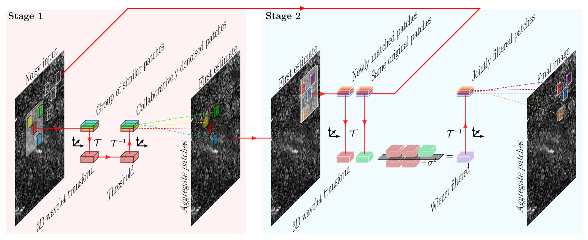
Figure 2 A schematic explanation of BM3D. In stage 1, similar looking patches are collaboratively denoised to produce a first denoised estimated image. In stage 2, similar looking patches are selected from the first estimate, and corresponding patches from the original input, form two blocks. Using a Wiener filter, the original image patches are denoised, leading to the final denoised image. The steps are carried out for all possible patches in the image.

BM3D denoises color images by forming a composite channel that contains the summed red, green, and blue image data. This composite channel is used for patch selection (step 1, above). For the remaining channels, the same patches are used, but each channel is denoised individually. We propose the same to make the process work for CO₂ and NO₂ images: we normalize the CO₂ and NO₂ images, and then form one channel of $({\mathrm{CO}}_{\mathrm{2}}+{\mathrm{NO}}_{\mathrm{2}})/\mathrm{2}$ and one channel of just NO₂. Patch selection is carried out on the first channel (the mean of the normalized CO₂ and NO₂ images), but denoising of the patches is carried out on both channels individually. By subtracting the second channel from the first, we end up with a new CO₂ image, which was helped by the higher signal-to-noise ratio of the NO₂ image during patch selection and denoising. A reference implementation in Python can be used that is called “bm3d” on pypi by Mäkinen et al. (2020).

2.3 Sequential denoising using the two presented methods

As the two methods (joint MMSE and BM3D) are sufficiently different in the structural features they use to denoise the data, it stands to reason that an application of both BM3D (to provide an initial cleaned up version of the data) followed by the joint MMSE (to further enhance the signal) will have the potential to further denoise the data. In this paper, we also test this sequential denoising method.

3 Results

3.1 Performance metrics

We score the performance of the methods where the truth is available using the two most common metrics in computer vision. The first is the peak signal-to-noise ratio (PSNR) in units of decibel, i.e. a higher value means a better performance,

$$\begin{array}{}\text{(13)}& \text{PSNR}=\mathrm{10}{\log }_{\mathrm{10}}\left({\displaystyle \frac{(max(c)-min(c){)}^{\mathrm{2}}}{\frac{\mathrm{1}}{n_x{n}_y}{\sum }_{i_x}{\sum }_{j_y}({\widehat{c}}_{i_x,j_y}-c_{i_x,j_y}{)}^{\mathrm{2}}}}\right),\end{array}$$

where $c\equiv c_{i_x,j_y}$ is the true (noise-free) signal and $\widehat{c}\equiv {\widehat{c}}_{i_x,j_y}$ is the estimated signal, indexed over all 2D pixels i_x and j_y. The second metric is the structural similarity index measure (SSIM; Wang et al., 2004, again, a higher value means a better performance),

$$\begin{array}{}\text{(14)}& \text{SSIM}(x,y)={\displaystyle \frac{(\mathrm{2}{\mathit{\mu }}_x{\mathit{\mu }}_y+c_{\mathrm{1}})(\mathrm{2}{\mathit{\sigma }}_{xy}+c_{\mathrm{2}})}{({\mathit{\mu }}_x^{\mathrm{2}}+{\mathit{\mu }}_y^{\mathrm{2}}+c_{\mathrm{1}})({\mathit{\sigma }}_x^{\mathrm{2}}+{\mathit{\sigma }}_y^{\mathrm{2}}+c_{\mathrm{2}})}},\end{array}$$

where x and y are 7×7 tiles/patches from images c and $\widehat{c}$ respectively, μ_x and μ_y are their sample averages, σ_x and σ_y are the sample standard deviations, σ_xy is their covariance, and $c_{\mathrm{1}}=\left(\mathrm{0.01}\right(max\left(c\right)-min\left(c\right)){)}^{\mathrm{2}}$ and $c_{\mathrm{2}}=\left(\mathrm{0.03}\right(max\left(c\right)-min\left(c\right)){)}^{\mathrm{2}}$. The PSNR is very sensitive to random noise, while the SSIM is very sensitive to image artifacts such as blurring. Consequently, we want the PSNR and the SSIM to improve simultaneously.

We can make a noise estimate using the algorithm described in Immerkaer (1996), which compares a grid-aligned Laplacian estimate with a diagonal Laplacian estimate, to estimate the noise standard deviation for Gaussian (i.e., white or random) noise as

$$\begin{array}{}\text{(15)}& {\mathit{\sigma }}_{\text{est}}=\sqrt{{\displaystyle \frac{\mathit{\pi }}{\mathrm{2}}}}{\displaystyle \frac{\mathrm{1}}{\mathrm{6}(W-\mathrm{2})(h-\mathrm{2})}}\sum _{\text{pixels}}\left|I(x,y)\ast N\right|\end{array}$$

where W and H, respectively, are the width and height of the trace gas image I, and where ∗ denotes a spatial convolution with the 2-D kernel

$$\begin{array}{}\text{(16)}& N=\left[\begin{array}{rrr}\mathrm{1}& -\mathrm{2}& \mathrm{1}\\ -\mathrm{2}& \mathrm{4}& -\mathrm{2}\\ \mathrm{1}& -\mathrm{2}& \mathrm{1}\end{array}\right].\end{array}$$

3.2 Application to synthetic joint CO₂ and NO₂ images

In this section, we will apply the algorithms presented above to synthetic CO2M CO₂ and NO₂ satellite images from the SMARTCARB dataset (Kuhlmann et al., 2020a, b). The SMARTCARB dataset is a synthetic quasi-Level 2 product at the CO2M spatial resolution (roughly 2×2 km²) and swath length (roughly 250 km) over primarily Germany and surrounding regions, for the year 2015. As it is essential that plume signals look “similar” for input to the MMSE methods, we will use column-averaged dry-air mole fractions of CO₂ (XCO₂) data (in ppmv) and tropospheric NO₂ column densities (in molec. cm⁻²). The reason for using XCO₂ rather than CO₂ column densities is that the latter are strongly susceptible to surface topography variations. One could also use XNO₂ images, but the topographic effect on NO₂ images is typically negligible. Hence, we will essentially use the “standard” data products. When denoting the results with the joint MMSE, the parameter T refers to the window size used to compute expected values within the joint MMSE method. For example, T=5 means that we select a 5×5 region centered on a pixel, which for CO2M is a region of about 10×10 km.

We will refer to results from the joint MMSE as “jMMSE” and from the BM3D method as “BM3D”. Additionally, we show the results from applying a simple 5×5 pixel mean filter (denoted as “5×5 mean filter” or “5×5 filter”) to purely the CO₂ data, which was proposed in Hakkarainen et al. (2022) as a simple but effective method to prepare the noisy SMARTCARB data for the divergence method. Figures 3–4 show an example of the denoising methods applied to synthetic CO2M CO₂ and NO₂ images. The examples use the “high noise” scenario of the SMARTCARB dataset with random errors of σ_VEG50=1 ppm for XCO₂ (the VEG50 scenario uses vegetation albedos and solar zenith angle of 50°; Buchwitz et al., 2013) and $\mathit{\sigma }=\mathrm{2}\times {\mathrm{10}}^{\mathrm{15}}$ molec. cm⁻² for NO₂. We select the simulation day 23 October 2015, and focus on the coal-fired power plants Prunéřov¹ and Počerady². These mid-sized power plants were selected as their emissions produce only weak plume enhancements compared to the CO₂ measurement noise level. Figure 3 shows that the simulated high noise on the CO₂ signal largely obscures the signal of the power plants, while the high noise on the NO₂ signal does not cause considerable changes with respect to the “true” simulated NO₂ field. We can see that the 5×5 pixel mean filter does not manage to recover much of the CO₂ signal. Conversely, applying the joint MMSE to the two noisy input fields recovers much of the CO₂ images for a window size T=9 – see Sect. S5 for images of other window sizes. The BM3D method (panel c) performs roughly equal to the joint MMSE method with T=9 (panel b). We obtain the highest objective score by sequentially applying the joint MMSE method with T=9 to the BM3D results (panel d), with a visibly good fit to the noisefree CO₂ signal, as well as an eightfold improvement of the SSIM and an increase in PSNR by +45.1 dB when going from the noisy image to the denoised image. To put this into context, consider that for Gaussian white noise, averaging X images with noise variance σ_noisy yields ${\mathit{\sigma }}_{\text{denoised}}^{\mathrm{2}}={\mathit{\sigma }}_{\text{noisy}}^{\mathrm{2}}/X$. Their PSNR improvement in dB may be expressed as $\mathrm{10}{\log }_{\mathrm{10}}\left({\mathit{\sigma }}_{\text{noisy}}^{\mathrm{2}}/{\mathit{\sigma }}_{\text{denoised}}^{\mathrm{2}}\right)=\mathrm{10}{\log }_{\mathrm{10}}\left(X\right)$. Using this relation, we we obtain here that $X={\mathrm{10}}^{\mathrm{45.1}/\mathrm{10}}\approx \mathrm{32}\mathrm{000}$, i.e., the image denoised with BM3D and jMMSE for T=9 has the same noise characteristics as if we would have averaged 32 000 images with these Gaussian independent high noise characteristics. Thus, the joint information content in CO₂ and NO₂ images is very large.

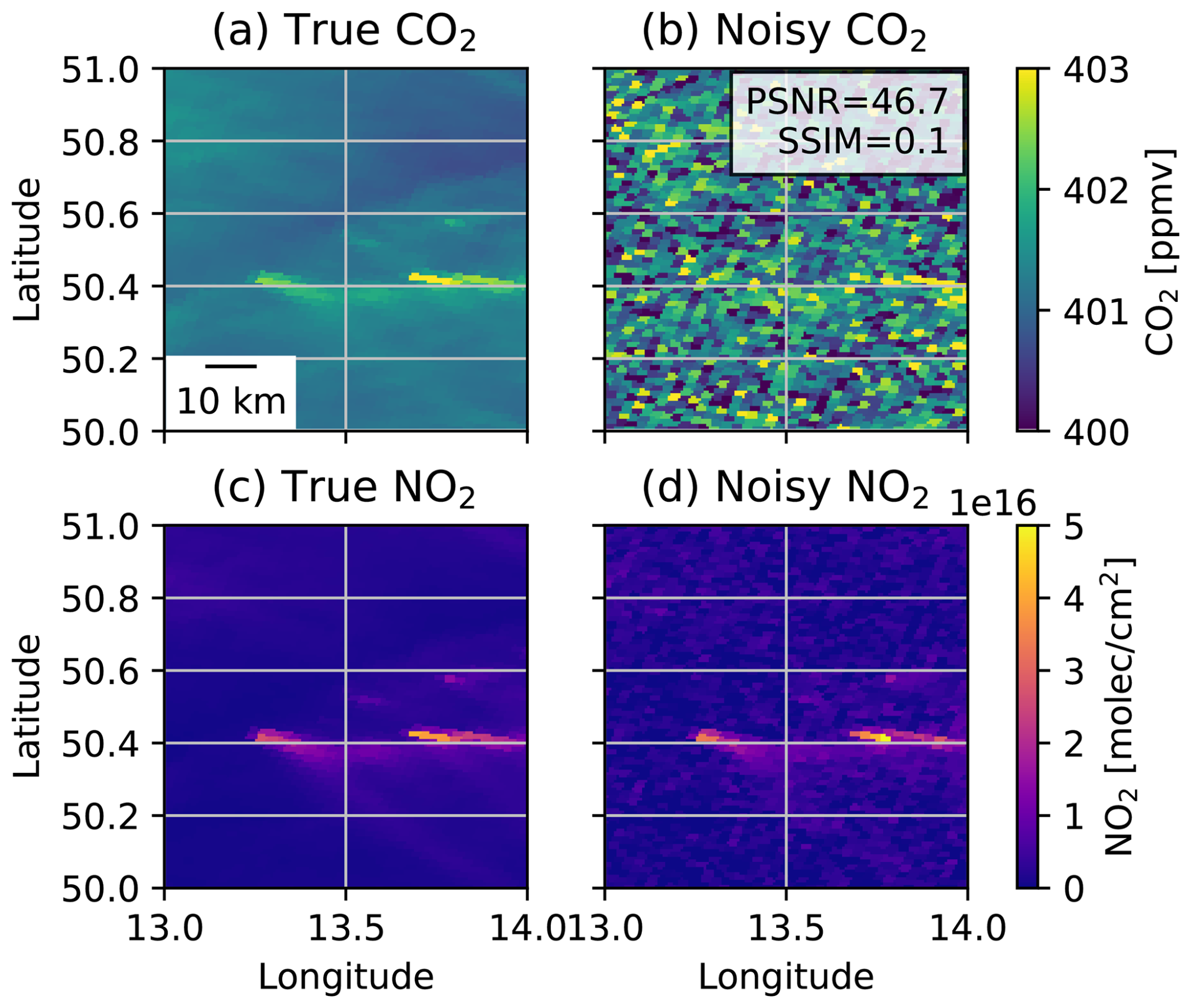
Figure 3 An example of a synthetic CO2M satellite image on 23 October 2015 for a “high noise” scenario zooming on the emission plumes of the coal-fired power stations near Prunéřov and Počerady.

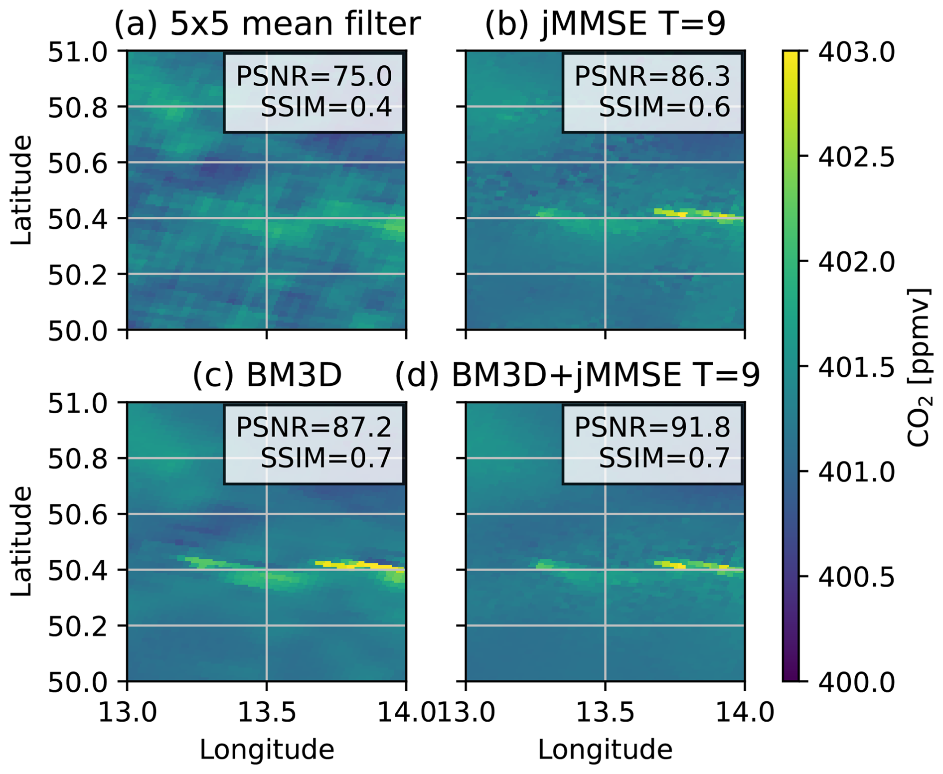
Figure 4 The noisy data from Fig. 3b denoised using the jMMSE methods. Visually, it is clear that the plumes originally obscured by noise become visible again. The PSNR and SSIM scores have increased (indicating improvement). The best denoising performance is obtained by the combination of BM3D and the jMMSE method for T=9, with a +45.1 dB improvement.

3.3 Application to joint SO₂ and NO₂ TROPOMI images

The method is also evaluated using Level-2 trace gas products from Sentinel-5P/TROPOMI, which provides near-daily global coverage at a spatial resolution of approximately 7×3.5 km² at nadir. We use reprocessed (RPRO) SO₂ data (processor version 02.04.01) and NO₂ data (processor version 02.04.00) for the year 2021 (Copernicus Sentinel-5P, 2020, 2021). We perform the denoising using a qa_value > 0.35 to retain some more data for the denoising methods to work with, but after denoising, we analyse and plot the results using the standard recommended threshold of qa_value > 0.75. The SO₂ product used here corresponds to the SO₂ Differential Optical Absorption Spectroscopy (DOAS) RPRO product. The more recent operational RPRO product is obtained using the Covariance-Based Retrieval Algorithm (COBRA), which has significantly lower noise and a corrected bias in the retrieval. As a consequence, the denoising performance demonstrated here for SO₂ should be interpreted in the context of this earlier processor version; results may differ for COBRA-based products due to their improved signal-to-noise ratio and potentially different error correlation structure. To better represent surface emissions, an air mass factor correction is applied to the SO₂ images, dividing the total column by the average of the three lowest averaging kernel weights³. While a more detailed investigation of air mass correction factors would benefit accurate emission estimates, that is beyond the scope of this study.

Figure 5a–d shows a TROPOMI overpass image over South Africa centered at Johannesburg for 3 March 2021, along with the ratio of the reported column precision to column values. This latter aspect is the inverse SNR (or, equivalently, the noise-to-signal-ratio). The NO₂ image has substantially larger regions of low inverse SNR values (indicative of a good SNR) than that found for SO₂. Hence, the SNR for NO₂ is much better than that for SO₂. Figure 5e shows that the SO₂ signal can be improved using the NO₂ signal with the multichannel BM3D method. The noise reduction becomes greater when the combination of the BM3D and jMMSE method is applied (panel f). Note that we use the jMMSE using T=5, which effectively implies a window of 25×24.5 km² at nadir, which is slightly larger than what we used for the SMARTCARB test. Figure 5g–h illustrates the changes compared to the original TROPOMI image, indicating substantial noise reduction. What is notable is that values close to 0 in Fig. 5g–h are exactly those regions with good SO₂ SNR as shown in Fig. 5d. Hence, denoising has primarily removed “bad” signal while preserving “good” signal. Furthermore, the removed noise as shown in 5g–h is essentially feature-less and consists of random speckles. Had we seen plume-like features in Fig. 5g–h we would know that we were subtracting signal and not just noise, but this is clearly not the case. Thus, subtracting the denoised image from the original image provides an easy way to check if signal was added or destroyed.

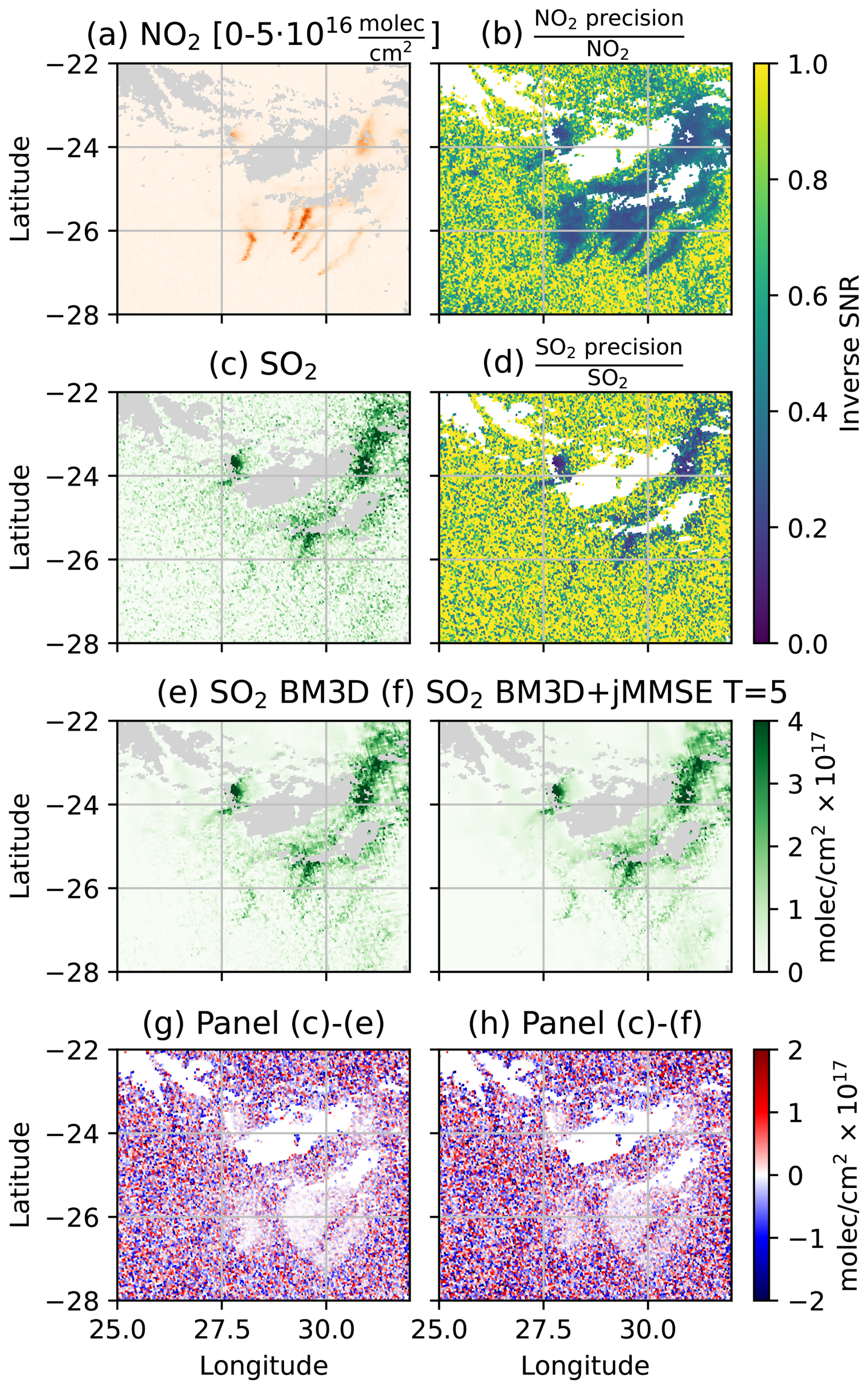
Figure 5 Single TROPOMI overpass image on 3 March 2021 of (a) NO₂ and (c) SO₂. All pixels with a qa_value larger than 0.75 are plotted. Panels (b) and (d) plot the inverse of an estimate of the SNR, where values close to zero are assumed to be of high SNR. Panels (e) and (f) show an application of the (multichannel) BM3D and additionally the jMMSE. Panels (g) and (h) show the difference between the estimates and the original SO₂ image.

If we apply the noise estimation method from Immerkaer (1996) to our image, we find that the original SO₂ image has ${\mathit{\sigma }}_{\text{est,original}}=\mathrm{4.1}\times {\mathrm{10}}^{\mathrm{24}}$ molec. cm⁻² (which is 1.7 times the mean reported column precision for this overpass), while ${\mathit{\sigma }}_{\text{est,BM3D}}=\mathrm{1.2}\times {\mathrm{10}}^{\mathrm{24}}$ molec. cm⁻² and ${\mathit{\sigma }}_{\text{est,BM3D+jMMSE}T=\mathrm{5}}=\mathrm{5.9}\times {\mathrm{10}}^{\mathrm{23}}$ molec. cm⁻²; in other words, a relative improvement of about 70 % or 86 %, respectively.

When considering a full year of observations (only selecting observations with a qa_value larger than 0.75) we find that the original SO₂ image has a mean noise estimate following the method of Immerkaer (1996) of ${\stackrel{\mathrm{‾}}{\mathit{\sigma }}}_{\text{est,original}}=\mathrm{4.2}\times {\mathrm{10}}^{\mathrm{24}}$ molec. cm⁻², the BM3D average estimated noise is ${\stackrel{\mathrm{‾}}{\mathit{\sigma }}}_{\text{est,BM3D}}=\mathrm{2.3}\times {\mathrm{10}}^{\mathrm{24}}$ molec. cm⁻², and ${\stackrel{\mathrm{‾}}{\mathit{\sigma }}}_{\text{est,BM3D+jMMSE}T=\mathrm{5}}=\mathrm{1.4}\times {\mathrm{10}}^{\mathrm{24}}$ molec. cm⁻² – that is, a 47 % and 66 % improvement in noise characteristics, respectively.

To further illustrate the advantage of this methodology, we present annual SO₂ divergence maps in Fig. 6, i.e., computations of ∇×(u_eff SO₂) averaged over a full year, where u_eff is the 2-D vector containing the effective horizontal wind. In this case, wind fields were computed by vertically averaging ERA-5 reanalysis fields using the GNFR-A emission profile as weights. (We present an identical analysis for the SMARTCARB dataset in Sect. S4 where we show that the denoising methods, with the exception of the 5×5 pixel mean filter, do not introduce any biases, supporting the validity of the denoising approach for emission quantification.) The divergence was computed on the TROPOMI overpass coordinate system, and then remapped to a common 0.03° grid. We consider the divergence map after applying BM3D to the overpasses in Fig. 6b, a 5×5 pixel mean filter to each TROPOMI overpass as suggested by Hakkarainen et al. (2022) in Fig. 6c, and the BM3D+jMMSE T=5 approach in Fig. 6d. The 5×5 pixel mean filter reduces noise but considerably smears the signal; in contrast, the other two methods better suppress noise while retaining source sharpness. Using the method of Immerkaer (1996), we observe a 94 % noise reduction with the 5×5 pixel mean filter, while the BM3D approach reduces noise by 49 % and the BM3D+jMMSE approach by 68 %.

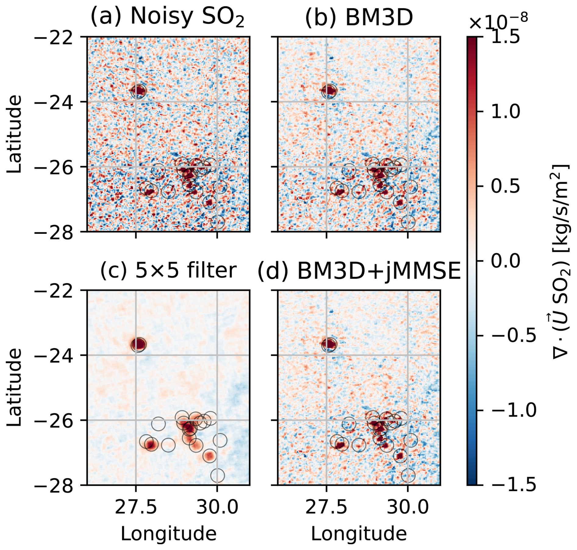
Figure 6 Annual divergence maps for a region in South Africa. (a) The original “noisy” TROPOMI SO₂ divergence map, (b) the estimate from applying BM3D to the SO₂ and NO₂ field prior to taking the divergence, (c) the estimate from a 5×5 mean filter to the noisy SO₂ prior to taking the divergence, (d) the estimate from the optimal SO₂ image using the proposed BM3D+jMMSE T=5 method prior to taking the divergence. A number of known sources are encircled.

To demonstrate that the denoising minimally impacts the signal structure, we compare emission estimates from different divergence fields in Fig. 7 (a more detailed examination of the estimates is provided in Sect. S5, where we also present a “difference” plot between the “noisy” divergence image and the denoised estimates). We focus on the ratio of the original “noisy” TROPOMI data estimates to those obtained with the denoising approaches. Emission estimates were obtained by spatial integration after masking data more than 0.15° from the point source location, corresponding to an integration radius of 16.7 km longitudinally and 15 km latitudinally. It is clear that the 5×5 pixel mean filter estimates significantly deviate from those based on noisy data. In contrast, estimates using the BM3D and BM3D+jMMSE T=5 approaches are closer to the noisy data estimates, although some deviation is present. Sources where these two methods significantly differ from the noisy data are weakly represented in the SO₂ and/or NO₂ dataset. This indicates that the noisy data may not accurately capture their presence and thus may not serve as reliable ground truth for comparison. In fact, the major deviations in Fig. 7, the Newcastle Steel Works and Camden Power Station, yield negative emissions when using the original noisy data. Therefore, the divergence method does not provide a reliable estimate of these source emissions in these cases. This may be due to a (combination of a) variety of reasons, e.g., there was not enough data to produce a robust average; there was a temporal bias in the sampling (the divergence method needs satellite images with plumes being blown in all directions to produce a “point” on a map; otherwise “dipoles” with seeming positive and negative sides appear – so if our overpass consistently samples cases where the wind is blowing in one direction, we will get artifacts); the steady state assumption was invalid; our chosen effective wind is not appropriate for the terrain and/or plume.

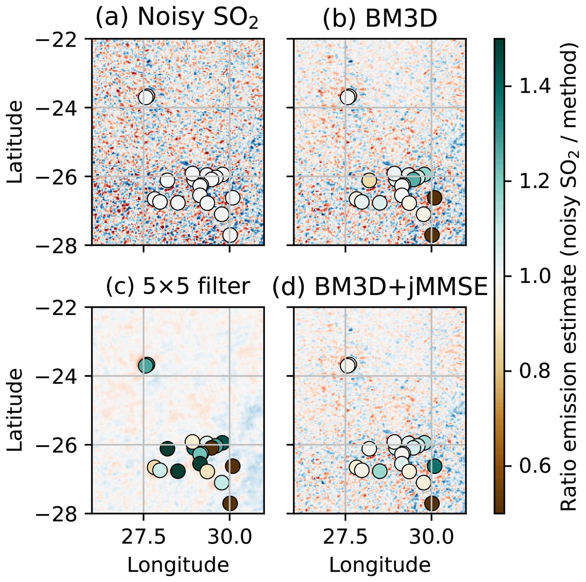
Figure 7 SO₂ emission estimate ratios from integrating along a ∼ 15 km radius around point source locations across the divergence maps shown in Fig. 6. A “blue” color in the ratio columns corresponds to an underestimation compared to the “noisy” SO₂ divergence map, while a “red” color in the ratio columns corresponds to an overestimation. Note, that the “noisy” SO₂ divergence map is not necessarily a ground truth, and this plot is shown for illustrative purposes only.

4 Discussion

The joint MMSE and BM3D approaches aim to denoise data while preserving the signal. The examples demonstrate the effectiveness of these methods, but they also have limitations.

Firstly, these methods assume independent and identically distributed (i.i.d.) noise with zero mean. Consequently, structural noise patterns, such as stripes, may not be denoised and could be misinterpreted as meaningful signals by BM3D due to the self-similarity of structural noise. While tuning BM3D for such cases is possible with prior knowledge of noise distribution in the 2D wavenumber domain (Mäkinen et al., 2020), this knowledge is often absent for satellite data. Another violation of the i.i.d. assumption may show up in the form of correlated errors in both satellite products due to shared dependencies in the radiative transfer (such as albedo, cloud contamination or aerosol loading). These factors enter both retrievals, thereby introducing a common-mode error component. Mitigation strategies could include restricting the analysis to scenes with low sources of such errors, or extending the statistical model presented here to include such correlated errors or biases. Consequently, users should interpret the denoised image with caution in regions where strong scene-dependent retrieval artifacts are expected, as these features, shared between the low and high SNR images, may be preserved or even reinforced in the denoised output.

Secondly, the practical implementation of jMMSE requires spatial stationarity, meaning the ratio of NO₂ : CO₂ column densities (or similarly chosen trace gases) should be approximately constant within a window of T×T pixels. It is clear that there is no globally fixed NO₂ : CO₂ ratio, and although this is approximately true when we focus on a small region, NO_x chemistry inside plumes will change ratios inside plumes (Meier et al., 2024; Krol et al., 2024). Hence, the value for T must be kept as low as possible. The competing interest, of course, is that for robust statistics, T should be chosen as large as possible. This raises the question of how to appropriately choose T. This can be based on subtracting the original image from the denoised image. Whatever shows up as structureless features there is noise, while whatever shows up as structured noise is likely the removal of real signal (e.g., this might happen if the difference shows something that looks like a plume and is indeed coincident with a plume on the original data). If one can grow T, but at some value of T the noise rejection does not improve anymore, then one has found the optimal T for noise rejection. Conversely, if one can grow T but at some point one is starting to reject also signal, then one can say they have found the optimal T to retain the signal. This argument suggests that spatial stationarity is best satisfied over small regions and indicates that denoising will be more applicable in high-resolution rather than coarse-resolution satellite images. The authors believe that rather than prescribing a value of T in this paper, it should remain an open hyperparameter for end users to decide. However, in the Supplement we demonstrate two example workflows for selecting the parameters based on a simple grid search – either by minimizing an objective function that maximizes noise reduction while minimizing signal bias, or by performing a simple grid search optimization for the remaining hyperparameters. Once optimal parameters are found to work for a handful of images, they generally work well for a full dataset.

5 Conclusions

We presented two minimum mean square error (MMSE) estimators that enhance the signal-to-noise ratio (SNR) of noisy CO₂ or SO₂ images using co-registered NO₂ images from the upcoming GOSAT-GW and CO2M satellites, as well as from Sentinel-5P. These methods enhance the visibility of plumes that are hard to discern in the noisy images. The first method, joint MMSE, preserves plumes with good SNR (i.e., where the signal is strong or highly correlated with the NO₂ field) while subtracting noise elsewhere. The second method, BM3D, leverages image self-similarity by denoising a linear combination of normalized CO₂ or SO₂ and NO₂ images. The best outcomes result from combining both estimators, initially applying BM3D for denoising, followed by joint MMSE for further refinement of the CO₂ or SO₂ image.

We demonstrate the effectiveness of these techniques in two case studies. In synthetic data tests, the denoising process improves peak SNR by more than 40 dB. When applied to TROPOMI SO₂ and NO₂ images over South Africa, or their annual divergence maps, we observe that a 30 %–60 % reduction in noise levels is possible, while leaving plume structures intact.

The proposed denoising methods can enhance plume detection for single-overpass images and averaged satellite datasets. These techniques improve plume visibility and may assist in plume emission quantification methods, such as Gaussian plume inversion, cross-sectional flux methods, or the divergence method, by providing cleaner input data. Therefore, by systematically reducing noise in total column images, this approach strengthens satellite capabilities for monitoring atmospheric emissions with greater precision.

Appendix A: Python implementation

In order to implement Eq. (11), we need to compute the quantities C_nn, C_dd and 𝔼[M] with sufficient accuracy. In this section, we give some possible ways to obtain these quantities.

1. The expected column 𝔼[M] can be defined as the median value of a T×T patch around any given pixel.

2. The data covariance matrix C_dd is defined by Eq. (5). To estimate it from the data (the “sample covariance matrix”), we form two row vectors of size 1×T² – for example, $\stackrel{\mathrm{̃}}{\mathit{C}{\mathit{O}}_{\mathrm{2}}}$ as a 1×T² row vector containing all $\stackrel{\mathrm{̃}}{{\mathrm{CO}}_{\mathrm{2}}}$ observations in a T×T patch around the pixel, and $\stackrel{\mathrm{̃}}{\mathit{N}{\mathit{O}}_{\mathrm{2}}}$ as a 1×T² row-vector containing all $\stackrel{\mathrm{̃}}{{\mathrm{NO}}_{\mathrm{2}}}$ observations around the pixel. Defining the sample deviation matrix as a 2×T² array, $\mathbf{M}=[{\stackrel{\mathrm{̃}}{\mathit{C}{\mathit{O}}_{\mathbf{2}}}}^T{\stackrel{\mathrm{̃}}{\mathit{N}{\mathit{O}}_{\mathbf{2}}}}^T{]}^T-\mathbb{E}[\mathit{M}]$, we may compute the 2×2 data covariance matrix,

   $$\begin{array}{}\text{(A1)}& {\left.{\mathbf{C}}_{dd}\right|}_{\text{sample}}={\displaystyle \frac{\mathrm{1}}{T^{\mathrm{2}}-\mathrm{1}}}{\mathbf{MM}}^T.\end{array}$$

   As we want to use a small value for T, it makes sense to use covariance shrinkage operators, which makes the estimation more robust (Ledoit and Wolf, 2022). A simple operation is to get the eigenvector decomposition ${\left.{\mathbf{C}}_{dd}\right|}_{\text{sample}}=\mathbf{U}\mathbf{\Lambda }{\mathbf{U}}^T$, and reconstruct it with modified eigenvalues as

   $$\begin{array}{}\text{(A2)}& {\left.{\mathbf{C}}_{dd}\right|}_{\mathrm{est}}=\mathbf{U}{\mathbf{\Lambda }}^{\prime }{\mathbf{U}}^T,\end{array}$$

   where ${\mathbf{\Lambda }}^{\prime }=(\mathit{\alpha }\mathbf{\Lambda }+(\mathrm{1}-\mathit{\alpha })$Diag$(n_{{\mathrm{CO}}_{\mathrm{2}}},n_{{\mathrm{NO}}_{\mathrm{2}}}))$ contains the modified eigenvalues based on the expected noise characteristics of the data, and Diag$(\times ,\times )$ forms a diagonal matrix with the elements given. For α=0.5 and $n_{{\mathrm{CO}}_{\mathrm{2}}}$ and $n_{{\mathrm{NO}}_{\mathrm{2}}}$ as diagonal entries of ${\left.{\mathbf{C}}_{dd}\right|}_{\text{sample}}$ we, for example, mix the sample covariance matrix and a diagonalized covariance matrix.

3. The noise covariance matrix C_nn corresponds to the precision of the instrument. If the noise is uncorrelated and known as ${\mathit{\sigma }}_{{\mathrm{CO}}_{\mathrm{2}}}^{\mathrm{2}}$ and ${\mathit{\sigma }}_{{\mathrm{NO}}_{\mathrm{2}}}^{\mathrm{2}}$ for the two measurements, that simply corresponds to ${\left.{\mathbf{C}}_{nn}\right|}_{\text{instrument}}$ = Diag$({\mathit{\sigma }}_{{\mathrm{CO}}_{\mathrm{2}}}^{\mathrm{2}},{\mathit{\sigma }}_{{\mathrm{NO}}_{\mathrm{2}}}^{\mathrm{2}})$. Alternatively, if this type of data is not available, we may estimate it as the median covariance of a single overpass (or image), the idea being that a typical image contains primarily “noise” and only a limited amount of “signal” (i.e., hot spot enhancements) such that the median covariance matrix of the data is representative for the noise.

We can give a straightforward example of an implementation of this algorithm in about 100 lines of Python code. Special care is taken of missing data through use of the numpy “mask” feature. Along with the robust estimator for C_dd, we also include the capacity to make sure C_dd has a stable inverse by clipping the conditioning number and by adding small values along its diagonal. The code given here is given as an example of how the quantities used in the theory could be computed in practice.

def covariance_shrinkage(Cdd, alpha, max_cond, min_eig):
    var_CO2 = np.ma.median(Cdd[:,:,0,0])
    var_NO2 = np.ma.median(Cdd[:,:,1,1])
    λ, U = np.linalg.eigh(np.nan_to_num(Cdd))
    λ[:,:,0] = alpha * λ[:,:,0] + (1-alpha) * var_CO2
    λ[:,:,1] = alpha * λ[:,:,1] + (1-alpha) * var_NO2
    eig_max = np.maximum(λ[:,:,1], min_eig)
    eig_min_allowed = eig_max / max_cond
    λ[:,:,0] = np.maximum(λ[:,:,0], eig_min_allowed)
    recon = (U * λ[..., None, :]) @ U.transpose((0,1,3,2))
    recon[np.isnan(Cdd)] = np.nan
    return recon

def ridge_regularization(Cdd, max_cond, γ, Γ):
    cond_num = np.linalg.cond(Cdd.filled(1.0))  # shape (lon, lat)
    p = 2.0  # curvature of ramp
    cond_factor = np.clip(np.log10(cond_num) / np.log10(max_cond), 0, 1)
    nugget_strength = γ + cond_factor**p * (Γ - γ)

    # Apply proportional nugget to each variance term
    Cdd[:,:,0,0] += nugget_strength * np.ma.median(Cdd[:,:,0,0])
    Cdd[:,:,1,1] += nugget_strength * np.ma.median(Cdd[:,:,1,1])

    variance_floor = np.ma.median( Cdd[:,:,0,0] )
    Cdd[:,:,0,0] = np.maximum(Cdd[:,:,0,0], variance_floor)
    return Cdd

def covariance(D, i, j):
    count = (D[i,...]*D[j,...]).count(axis=-1) - 1
    return np.ma.sum(D[i,...]*D[j,...], axis=-1)/count

def nanaverage(A,W,axis=-1):
    return np.nansum(A*W,axis=axis)/((~np.isnan(A))*W).sum(axis=axis)

def MMSE_estimate_fixed(
    in_arr1, in_arr2, T, CNN=None, alpha=0.5,
    method='median', max_cond=1e7, min_eig=1e-13,
    γ=1e-3, Γ=1e0):

    # --- Pad data (s.t. our windows catch all the data)
    CO2 = np.pad(in_arr1, ((T, T), (T, T)), 'symmetric')
    NO2 = np.pad(in_arr2, ((T, T), (T, T)), 'symmetric')

    # --- Extract overlapping patches of size WxW
    CO2_tiles = view_as_windows(CO2               , (T,T))
    NO2_tiles = view_as_windows(NO2               , (T,T))
    mask_tile = view_as_windows(~np.isnan(CO2+NO2), (T,T))

    # --- Reshape
    mask_tile = mask_tile.reshape(*mask_tile.shape[:-2], -1)
    X = np.stack((CO2_tiles.reshape(*CO2_tiles.shape[:-2], -1),
                  NO2_tiles.reshape(*NO2_tiles.shape[:-2], -1)))

    # --- Generate masked array
    X = np.ma.array( X, mask=~np.stack([mask_tile] * 2, axis=0) )

    # --- Compute expected value of the dataset
    av_field = {"mean": np.nanmean(X,-1,keepdims=1),
                "median": np.nanmedian(X,-1,keepdims=1)}[method]

    # --- Compute sample covariance matrix
    D = X - av_field
    Cdd = np.ma.zeros((*D.shape[1:3], 2, 2)) * np.nan
    Cdd[...,0,0] = covariance(D, 0, 0)
    Cdd[...,0,1] = covariance(D, 0, 1)
    Cdd[...,1,0] = covariance(D, 1, 0)
    Cdd[...,1,1] = covariance(D, 1, 1)
    Cdd = covariance_shrinkage(Cdd, alpha, max_cond, min_eig)
    Cdd = ridge_regularization(Cdd, max_cond, γ, Γ)

    # --- Compute noise covariance matrix
    Cnn = np.zeros_like(Cdd)
    Cnn[:,:,0,0] = np.ma.median(Cdd[...,0,0])
    if CNN is None:
        pass
    elif type(CNN) is np.float32:
        Cnn[:,:,0,0] = Cnn[:,:,0,0]*0.5 + CNN*0.5
    else:
        CNN = np.pad(CNN, ((T, T), (T, T)), 'symmetric')
        CNN = view_as_windows(CNN, (T,T))
        CNN = CNN.reshape(*mask_tile.shape[:-1], -1)
        CNN = np.nanmedian(CNN, -1)
        Cnn[:,:,0,0] = Cnn[:,:,0,0]*0.5 + CNN*0.5

    # --- Apply filter
    wCddICnn = np.linalg.solve(Cdd.filled(np.nan),Cnn.filled(np.nan))
    wCddICnnEM = np.einsum('ijk,kijl->ijl',wCddICnn[...,0].squeeze(),D)

    est_gather = np.zeros((*CO2.shape, T**2)) * np.nan
    for i in range(T**2):
        y, x = np.mod(i,T)-T//2, i//T-T//2
        xs, xe = max((T//2)+x,0), min(CO2.shape[0]-(T//2)+x, CO2.shape[0])
        ys, ye = max((T//2)+y,0), min(CO2.shape[1]-(T//2)+y, CO2.shape[1])
        est_gather[xs:xe, ys:ye, i] = wCddICnnEM[:,:,i]

    # --- Generate filter grid coordinates
    y, x = np.meshgrid(np.arange(-T//2+1, T//2+1), np.arange(-T//2+1, T//2+1))
    weights_2dgauss = np.exp(-(x**2 + y**2) / (2 * 4**2))

    # --- Compute final output
    pred = CO2 - nanaverage(est_gather,W=weights_2dgauss.flatten())
    est = np.where( np.isfinite(CO2), pred, np.nan )
    est = np.where( np.isnan(NO2) & np.isnan(est), CO2, est )

    return est[T:-T,T:-T]