Towards automated near-real-time global monitoring of atmospheric SO₂ plumes from satellite data using U-Net segmentation

Sulphur dioxide (SO₂) is a major atmospheric pollutant from fossil fuel combustion, metal smelting, and volcanic degassing, impacting human health, acid deposition, and climate forcing. Existing emission inventories are often temporally lagged and spatially coarse, failing to capture high-intensity, sporadic events. To address this, we present a novel, near real-time approach using a U-Net image segmentation model to automatically isolate SO₂ plumes from over 31 000 TROPOMI satellite swaths (January 2019–December 2024). The model successfully identified 53 993 individual plumes. The highest annual detection rate in 2019 was attributed to massive stratospheric SO₂ injections from the Raikoke and Ulawun volcanic eruptions. Clustering analysis confirmed plume origins around expected volcanic and industrial hotspots (e.g., Popocatépetl, Norilsk), with volcanic sources dominating the top ten clusters. However, the algorithm struggles to detect sources in high-background regions like China, where high SO₂ saturation likely prevents individual plume isolation. This study demonstrates machine learning as a powerful tool for transforming atmospheric monitoring, providing the high-cadence, fine-grained quantification of SO₂ emissions crucial for validating global inventories and ensuring effective environmental management.

1 Introduction

Sulphur dioxide (SO₂) is an atmospheric pollutant predominately produced from fossil fuel combustion for power generation, residential heating, industrial processes (e.g. metal smelting), refineries, shipping, and volcanoes. Within the clean troposphere, the dominant loss of atmospheric SO₂ is oxidation by the hydroxyl radical, resulting in a lifetime of approximately a week although this can vary dramatically depending on environmental conditions. SO₂ contributes to the formation of fine particulate matter that is directly linked with negative health outcomes, particularly cardiovascular diseases (Khalaf et al., 2024). SO₂ also has broader environmental impacts, primarily by forming sulphuric acid via heterogeous chemistry, which leads to ecosystem damage and building corrosion. The formation of sulfate aerosols affects climate forcing both directly, by scattering incoming sunlight and causing a net cooling of the atmosphere, and indirectly, by perturbing cloud microphysics. In this study, we use machine learning to identify automatically permanent and ephemeral hotspots of SO₂ observed by the TROPOMI satellite instrument and quantify the corresponding emission estimates, carefully curating sources of error. We will focus on large point sources from fossil fuel combustion, copper smelting, and volcanic emissions.

Emissions of SO₂ from fossil fuel combustion hinges on three factors: the sulfur content of the fuel, combustion efficiency, and the deployment of SO₂ scrubber technology. More energy is released during the combustion of coal with a higher number of hydrogen : carbon bonds, which is inversely proportional to the sulfur content. Scrubber technology, widely adopted by coal-fired power plants in developed nations starting in the 1990s (Srivastava et al., 2001), was introduced to meet regulatory requirements to mitigate acid deposition that caused widespread destruction of downwind forest and aquatic ecosystems (Smith, 1872; Driscoll et al., 2001). Global anthropogenic SO₂ emission estimates varied from 93 to 108 Tg yr⁻¹ between 2010 and 2018, with recent years showing lower values (Soulie et al., 2024). While different inventories, such as the Copernicus Atmosphere Monitoring Service (CAMS) and the Emissions Database for Global Atmospheric Research (EDGAR), generally agree within ≃ 4 Tg SO₂ yr⁻¹ estimates diverge in later years, primarily due to differing estimates for power generation (≃ 44 % of CAMS anthropogenic emissions during 2010—2018) and shipping (≃ 10 %). International shipping is a significant source due to the high sulfur content of marine fuel, but low-sulfur fuel regulations introduced in 2020 are expected to have significantly reduced this annual emission, consistent with a large reduction in observed ship tracks in cloud perturbations (Watson-Parris et al., 2022).

Extracting copper from mineral ores – predominately chalcopyrite (CuFeS₂) – releases SO₂ to the atmosphere. The smelting process involves injecting mineral particles and oxygen-enriched air into a furnace that is heated ≃ 1500 K, resulting in the sulphide minerals reacting with the injected oxygen that eventually produces SO₂. Currently, most copper refineries are in China, India, Japan, Russia, and Chile, with only a few smaller-capacity plants in the United States and Germany. Developed countries capture the SO₂ waste product but for refineries in developing countries the capture technology may be unaffordable or unavailable.

Volcanoes represent a natural source of SO₂ to the atmosphere. They emit SO₂ in vast quantities during eruptive and during passive degassing periods. Sulphur species is a minor constituent in volcanic magma, compared with water and carbon dioxide. The production and subsequent emission of SO₂ from volcanoes depends on various factors, including the composition and depth of the magma reservoir and the nature of the eruption. Generally, large, explosive (high pressure) volcanic eruptions release more SO₂ to the atmosphere than passive degassing periods, which occur due to the movement of sub-surface magma. Annual volcanic SO₂ emission estimates vary. Estimates inferred from satellite data collected between 2005 and 2015 report an annual mean of 23 ± 2 Tg yr⁻¹ for volcanic degassing, with 30 % of those sources exhibiting a positive decadal trend (Carn et al., 2017). However, ground-based data collected at 32 volcanoes over the same period report a mean (median) emission rate of ∼ 9.0 (6.8) Tg SO₂ yr⁻¹ (Arellano et al., 2021), and a subset of these ground-based estimates show that some volcanoes degas at a rate too low to be detected by instruments like the Ozone Monitoring Instrument (Carn et al., 2017). Only within the past decade has space-borne sensor technology achieved sufficient sensitivity to accurately detect degassing SO₂ emissions, providing crucial data that complements information gathered by ground-based networks, such as the Network for Observation of Volcanic and Atmospheric Change (Galle et al., 2010).

Traditional bottom-up emission inventories for SO₂ (e.g., EDGAR (EDGARv8.1, 2026), CEDS (Hoesly et al., 2018)) suffer from critical limitations for modern monitoring, including significant time lags (often years behind real-time) and poor resolution, providing only mean values over large areas (e.g., 100s of kilometres) and long durations (e.g., monthly). Capturing sporadic emission events or tracking rapid changes in current sources requires the high temporal resolution offered by near real-time satellite observations, especially emerging data from geostationary instruments (e.g. Global Environmental Monitoring Systems (GEMS; Kim et al., 2020), Tropospheric Emissions: Monitoring of Pollution (TEMPO; Chance et al., 2019) and Sentinel-4 (Bazalgette Courrèges-Lacoste et al., 2017)) that offer continuous monitoring throughout the sunlit day. To efficiently exploit these massive stream of data, we employ a machine learning model that rapidly highlights SO₂ plumes originating from point sources and an example of how to quickly estimates their emission rates. This capacity for rapid, fine-grained quantification of emission changes is essential for timely intervention and effective atmospheric management. We showcase our approach using data collected by the Tropospheric Monitoring Instrument (TROPOMI) satellite instrument aboard Sentinel-5P.

In the following section, we describe the data used and the development of the model. In Sect. 3 we report our result. We conclude the study in Sect. 4.

2 Data and Methods

2.1 TROPOMI SO₂

We use Level 2 total vertical column density (VCD) SO₂ data retrieved from TROPOMI, a high-resolution UV–Vis–NIR–SWIR spectrometer, onboard the Sentinel-5P satellite, January 2019–December 2024, inclusively. TROPOMI measures the solar radiation backscatter in the UV range (around 310–330 nm) where SO₂ has a distinct absorption feature. This analysis uses the TROPOMI Differential Optical Absorption Spectroscopy (DOAS) retrieval (Theys et al., 2017) from version 3 of the offline analysis product. Sentinel-5P was launched in October 2017 into a sun-synchronous orbit with a local equatorial overpass time of 13:30. TROPOMI has a swath width of 2600 km divided into 450 across-track pixels, with a pixel resolution of 3.5 × 5.5 km (across × along track) at nadir for SO₂ (increased from a resolution of 3.5 × 7 km from 6 August 2019). This sampling strategy results in near-daily global coverage (Veefkind et al., 2012), subject to cloud-free scenes. In this study, we only use pixels with a quality flag > 0.5, as recommended by the TROPOMI Level 2 Product User Manual (Romahn et al., 2024). No further filtering was applied to the data. Because this study uses the full VCD rather than the 1, 7 or 15 km layer products, we acknowledge that some potential SO₂ plumes located above cloud tops may be missed when applying a quality-flag threshold of 0.5. The broader implications of using the full VCD instead of layer-specific products are not assessed here, but this could be incorporated into future model developments and retrieval-selection strategies. A further development to explore in future work is the use of the Covariance-Based Retrieval Algorithm (CORBA) developed by Theys et al. (2021). The COBRA retrieval method has been shown to reduce noise and biases in the SO₂ column when compared with the DOAS method and would therefore likely impact the plume detection results. The comparison between DOAS and COBRA is not presented here due to data availability at the time of analysis.

An existing SO₂ detection flag is provided in TROPOMI files as described in the Sentinel-5P/TROPOMI Algorithm Theoretical Basis Document (Theys et al., 2023) built on a detection algorithm (Brenot et al., 2014). This detection algorithm combines the SO₂ observation, solar zenith angle, VCD error and proximity to other detections to assign a flag to each pixel. This flag uses five categories: (0) no enhancement, (1) general SO₂ detection, (2) near a known volcano, (3) near a known anthropogenic source, and (4) a potential false positive due to a high solar zenith angle. This study does not include this flagging data in training the model as we want the model to learn SO₂ enhancement and plume shapes without relying on existing methods. The flags indicating if the detection are near a known source (flags 2 and 3) also rely on proximity to a known source, which could adversely affect the ability of model to detect plumes from new sources. Our plume detection model is designed to be distinct from the detection flag by not relying on proximity to known sources and looking at plumes as a whole structure, rather than a pixel-by-pixel basis. We compare the results from our plume detection model with SO₂ flag provided in Sect. 3. The method presented in this study does not assign a threshold to a potential plume and tests whether a model can learn to correctly identify plumes from the TROPOMI data without pre-defined limits.

2.2 U-Net Image Detection Model

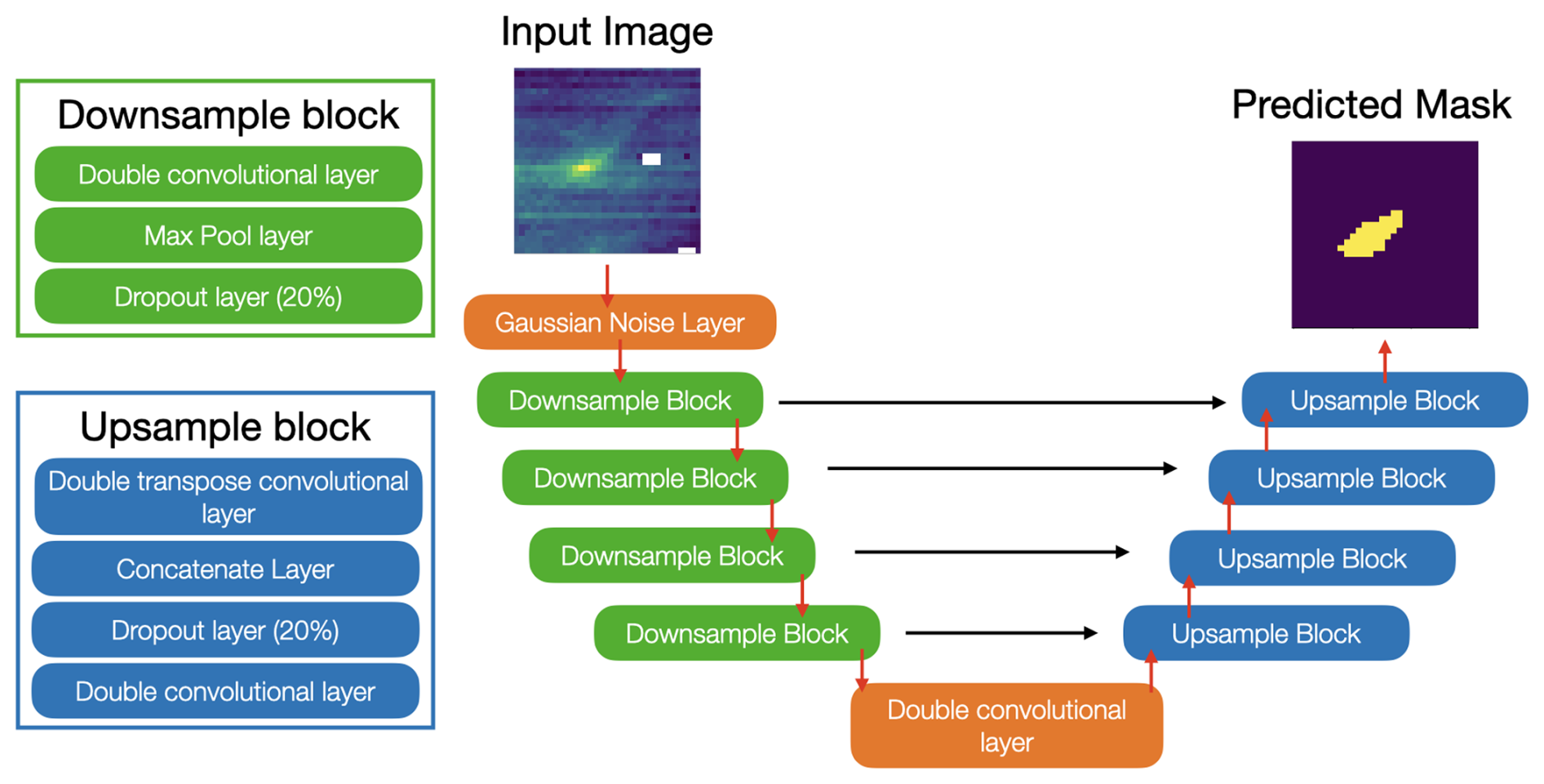
To automatically detect plumes of SO₂ from TROPOMI data, we use a U-Net style fully convolutional network model to perform image segmentation (Ronneberger et al., 2015; Mukhopadhyay et al., 2015). A U-Net model is designed to produce a pixel-by-pixel classification of an image and has been widely used in medical sciences (e.g. tumour detection) as well as in land cover classification in satellite imagery (e.g. Pan et al., 2020; Ulmas and Liiv, 2020; Bokstaller et al., 2021; Filatov and Yar, 2022). It follows the basic principle of convolving an image over successive layers to reduce the spatial dimensions and extract feature information and then using transposed convolutions to rebuild the image to the original shape, the schematic of the model architecture creates a “U” shape, as shown in Fig. 1. This figure shows a schematic of the model architecture used for the plume detection algorithm. We add Gaussian noise to the training images to improve the robustness of the model before passing the image through four downsampling blocks. Each block consists of a double convolutional layer, a max-pooling layer and a dropout layer set at 20 %. These blocks then feed to one more double convolutional layer to extract patterns in the image before four upsampling blocks create a mask of the plume. Each upsampling block contains a double transpose convolutional layer, a concatenation layer, another dropout layer set at 20 % and a double convolutional layer.

Figure 1 Schematic of the architecture of the U-Net model.

This architecture was based upon the original U-Net designs described in Ronneberger et al. (2015) then manually adapted through iterative tuning to fit this study. We found training the model for 20 epochs sufficient for our relatively simple image problem. We found no further model improvement when it was trained over more epochs. As our training dataset was relatively small (∼ 1000 images), we chose a batch size of 64 to balance over-fitting with training efficiency. The model uses a sigmoid activation as we wanted the model to make a binary pixel-wise classification of within a plume or not.

Image segmentation models offer significant advantages over traditional image classification (e.g. Finch et al., 2022) because they parse essential information from the background rather than simply assigning a single label to an entire image. For detecting SO₂ plumes, this capability is crucial: it allows for more precise geolocating of the plume and the ability to handle multiple distinct plumes within a single satellite scene. Furthermore, segmentation excels over other feature-parsing methods, such as activation maps (Zhou et al., 2015), because it is trained directly on ground-truth image masks. This direct comparison during training provides a clear, quantifiable performance metric, ensuring reliable results.

Our segmentation model was trained using a custom database of over 1000 TROPOMI images showing SO₂ plumes, each paired with a precise plume mask manually created by the lead author. These images were sampled randomly from all available TROPOMI files across the full study period and the global domain to minimize the risk of introducing geographical biases. While it would be possible to generate modelled plumes and corresponding masks for training, providing labels and complete background removal, this approach may introduce errors by misrepresenting observed plume characteristics. Consequently, we restrict training to SO₂ plume data derived from TROPOMI data.

The model is designed to detect single plumes and is not currently able to distinguish between multiple plumes that have merged (e.g. from nearby sources). Training the model to identify and separate merged plumes would require hundreds to thousands of additional examples, with merged plumes subdivided at the labelling stage, thereby introducing further potential for subjective error. More detail on the creation of the training dataset is provided in Appendix A. To maximize the effectiveness of training, we augmented this dataset through rotations and flips, yielding a final training pool of over 4000 images and corresponding masks. This dataset size is sufficient to demonstrate the capabilities of this method. Unlike classification models (e.g., Finch et al., 2022), including images without plumes is not necessary for the training of segmentation models. As we are training the model to be interested in part of an image, the model learns the background of images (i.e. outside the area/object of interest) as the ‘no plume’ case.

We chose an image size of 32 × 32 pixels (roughly 112 × 176 km² at nadir) as it successfully captures most SO₂ plumes. The computational cost for increases slightly more than linearly with image size. Doubling both dimensions typically increases the cost by about four times. Images this size correspond to plumes approximately 90 km in length. We find this is more than adequate for encompassing the majority of plumes For validation, we trained the model on 80 % of the data and tested it on the remaining 20 %. The model's performance was measured using precision (correctness of positive predictions) and recall (completeness of positive detection), yielding scores of 65.7 % and 74 %, respectively, giving an F1 score of 0.69. Crucially, the small 32 × 32 image size disproportionately penalizes minor errors, meaning an offset of just a few pixels drastically lowers the score. Although these scores indicate the performance of the model, the precision and recall percentages are not directly interpretable as plumes missed or not, as segmentation models work on a pixel per pixel basis. For example, the model may correctly detect a plume in the test dataset but draw a smaller or larger mask than the test data and would therefore be penalised. It is for this reason that we cannot directly compare these performance metrics to plume classification models (e.g. Finch et al., 2022). It is also important to note that because the training dataset was created manually and relied on the authors’ judgement of what constitutes a plume, the model cannot outperform the quality of this dataset. Any biases or recurring misclassifications present in the training examples may be learned by the model and subsequently propagated into the final results. An alternative approach would be to augment the training dataset with model-simulated SO₂ plumes, but for this study we chose to rely exclusively on real data to maximise the diversity of scenes and plume morphologies that may not be captured in model simulations.

To ensure we capture SO₂ plumes that may be straddling multiple image boundaries, we employ a 32 × 32 pixel rolling window that moves four pixels at a time across and along the satellite swath. This systematic sampling generates approximately 100 000 images per swath for input into the segmentation model. The model returns each image with a pixel-by-pixel probability of plume presence. We then reconstruct the original swath into an amalgamated mask by taking the median probability of all overlapping pixels. Using the median not only combines the individual predictions but also boosts detection confidence, as an accurately identified plume will appear consistently across multiple overlapping images. We found that a four-pixel step provides adequate coverage to resolve straddling issues while maintaining reasonable computing speed and costs. Crucially, this overlaying method means the final predicted plume shape is not limited by the 32 × 32 pixel input size, allowing plumes and their corresponding masks to be accurately mapped across the full scale of the swath (which is typically 4172 × 450 pixels, spanning 2600 km from pole to pole).

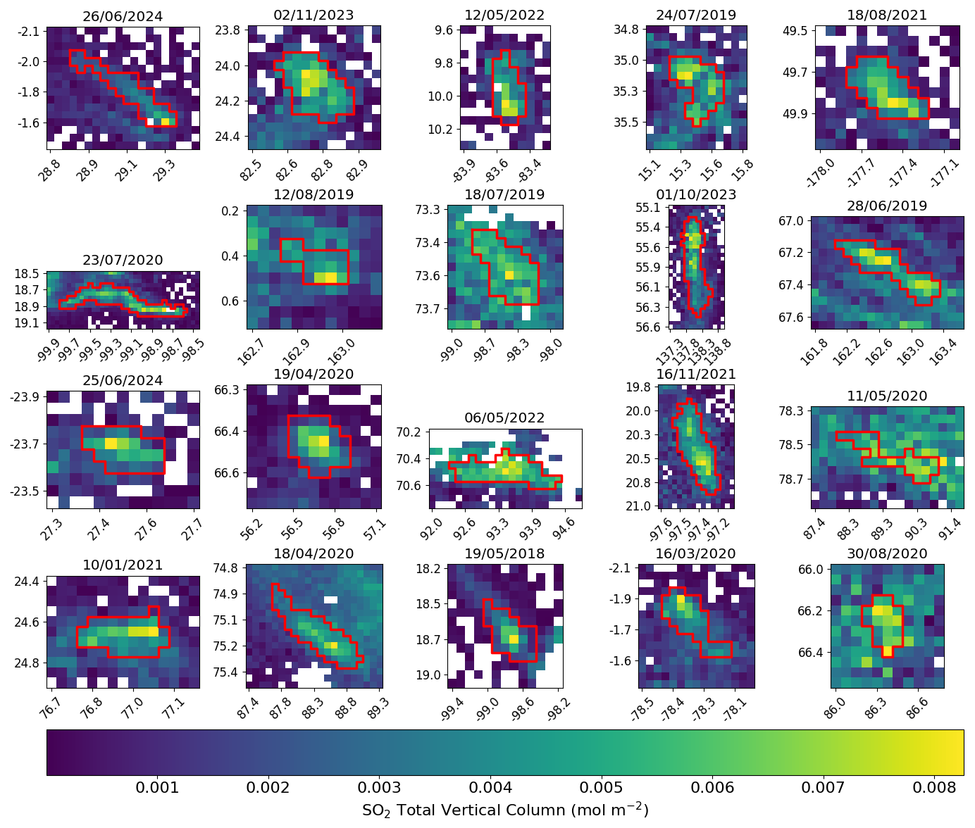
Figure 2 Examples of SO₂ plumes in the TROPOMI data and the predicted plume outline, shown as a red line. The title of each image shows the date of observations and the x and y axes are longitude and latitude, respectively.

To extract the details of individual plumes from the reconstructed satellite swath, we apply connected component analysis (using Open-CV; Bradski, 2000) to the pixel probability array. This analysis effectively identifies the unique plume masks within the swath and provides the bounding boxes for each one, allowing us to precisely delineate the plume outline. Figure 2 illustrates this capability, showing twenty randomly selected TROPOMI-observed plumes alongside their corresponding predicted plume outlines. The images in this figure show the varying sizes of the plume images, and that they are not limited to the 32 × 32 pixel training image size.

Figure 2 demonstrates that the model generally performs well, although some inaccuracies are present. Detecting atmospheric features like SO₂ plumes inherently involves subjectivity, as there is no clear, objective physical boundary for the feature of interest. This human subjectivity is inevitably encoded in the model's training dataset and subsequently reflected in the trained model itself. Continuously refining the model or updating the training dataset is an endless task, so for the practical scope of this paper we have chosen to present results based on a rigorous process involving three training iterations (i.e., checking model output, expanding the dataset with new examples, and retraining).

We have created a comprehensive database documenting each detected plume, which includes its location, date of detection and plume outline. We also estimate the length of the plume, based on taking the length of the primary axis of an ellipse fitted to the plume outline. We find the detected plumes have a median plume length of 37.5 km, much shorter than the length of the model input image. A bounding box (with a three-pixel buffer) is also recorded, with its limits specifically used to determine the background SO₂ concentration outside the plume. Computationally, processing a single swath is highly efficient, taking only about 15 s using a GPU or 60 s using CPUs.

3 Results

3.1 Global SO₂ Data

We processed approximately 31 000 Level 2 files from TROPOMI observations spanning January 2019 to December 2024. To ensure the reliability of our output, we implemented a filter requiring each detected plume to contain a minimum of six pixels, as the accuracy of smaller predicted plumes is difficult to validate.

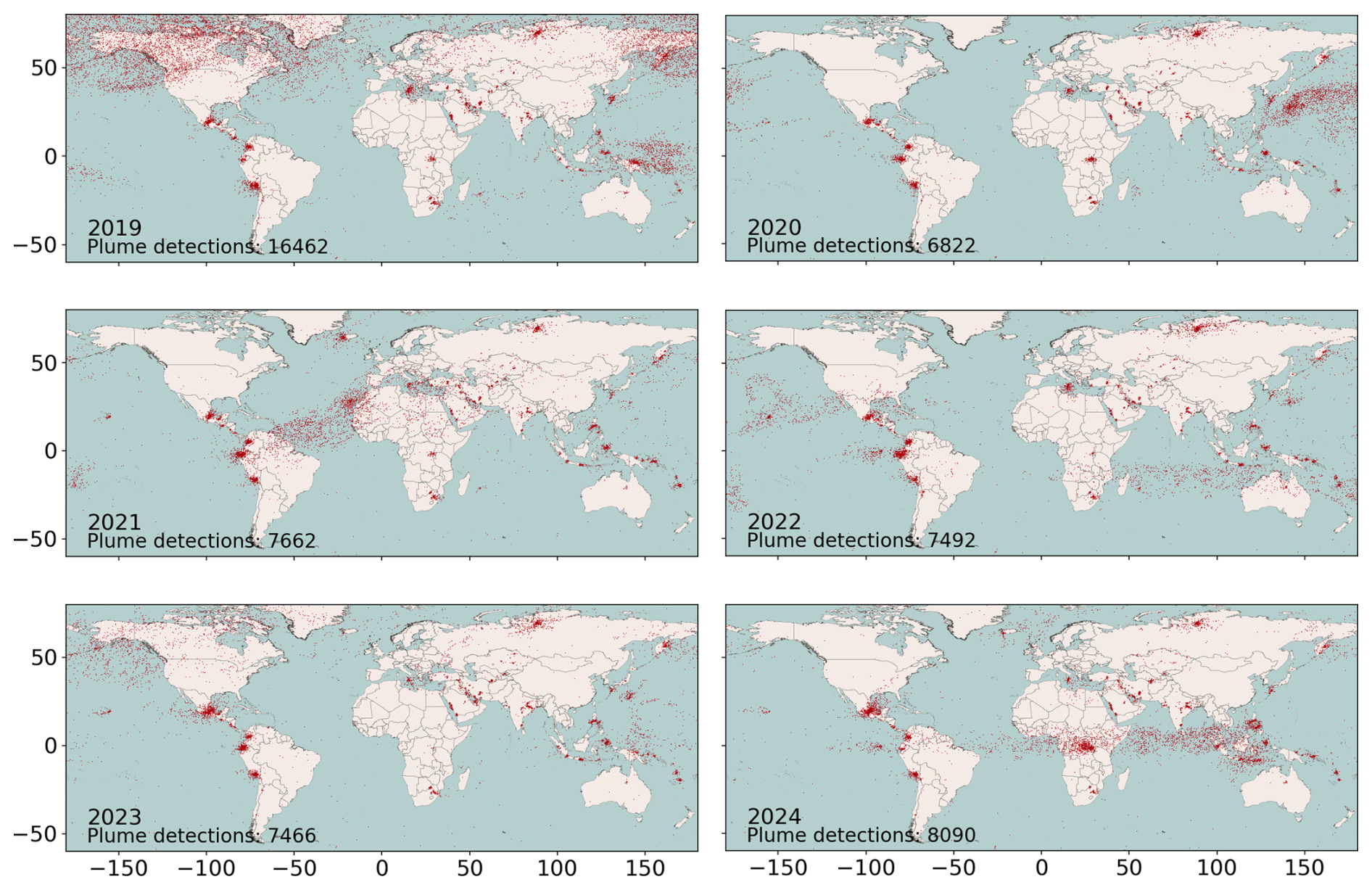
Figure 3 Global, annual locations of the maximum concentration of TROPOMI SO₂ within the predicted plume masks, 2019–2024.

In total, 53 993 plumes were identified over the study period. The year 2019 saw the highest number of detections, exceeding 16 000, while the period from 2020 through 2024 showed more consistent annual counts, ranging from ∼ 6800 to ∼ 8000 plumes. To locate the emission source, we employ the coordinates of the maximum SO₂ concentration within the plume boundary as a practical proxy for the origin, noting that this might not perfectly match the true source location. Figure 3 shows the annual global distribution of these estimated plume origins, 2019–2024.

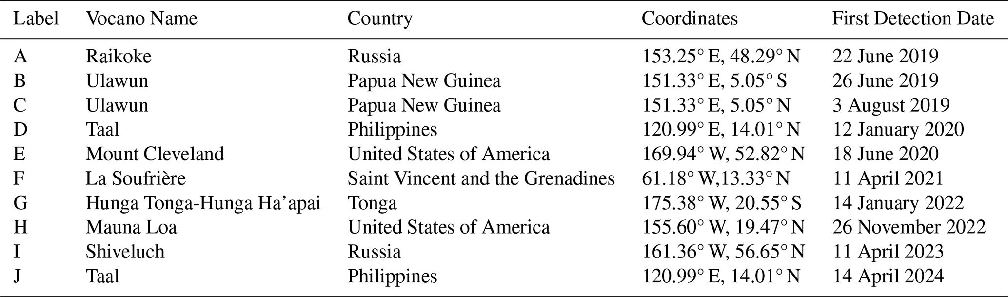
Table 1 Major volcanic eruptions thought to be responsible for the periods of higher than usual plume detections highlighted and labelled in Fig. 4.

Initial inspection confirms plumes cluster predictably around known volcanoes and industrial hotspots. However, all years also show regions with a wide, “noisy” spread of detections (e.g., Alaska, Canada, and Eastern Russia annually, plus specific areas like the mid-Atlantic in 2021 or Central Africa in 2024). Figure 4 illustrates the daily plume counts, where each spike corresponds to these noisy geographical spreads (Fig. 3). Critically, all but one spike (Peak I in 2023) align with major volcanic eruptions in the region. Table 1 details the specific volcanic emissions believed responsible for this widespread geographical dispersal. Plume transport away from the source is evident, as detections further from the origin often occur in the days immediately following an eruption event (see Appendix B, Fig. B1).

We attribute the major spike in 2019 plume detections mostly to the coinciding eruptions of Raikoke, Russia, and Ulawun, Papua New Guinea. The Raikoke eruption on 21 June is particularly notable, injecting one of the largest amounts of sulfur dioxide (SO₂) into the stratosphere since the 1991 Mount Pinatubo eruption (Vernier et al., 2024, and references therein).

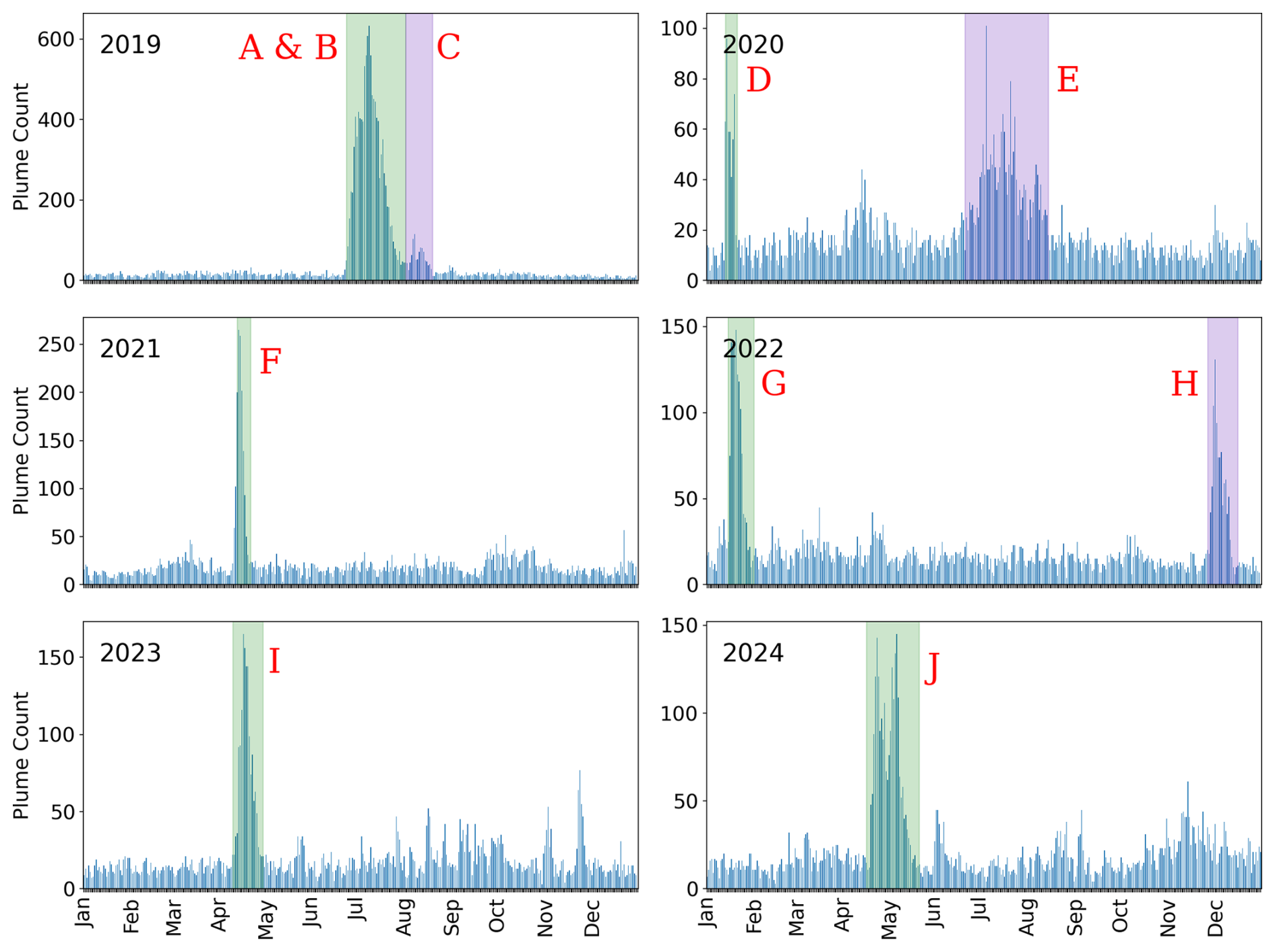
Figure 4 Number of plume detections per day for each year of the study. Highlighted regions show time periods of a higher than usual number of detections. Labels correspond to Table 1.

While Peak I in Fig. 4 corresponds to the Shiveluch eruption in Russia on 11 April 2023, it also coincides with a surge in detections concentrated over Norilsk in Northern Russia (88.1° W, 69.3° N), as shown in Fig. 5. This region is a known major source of SO₂ emissions due to its large metal smelting operations. The precise cause of this specific increase in plume detections, however, remains unknown.

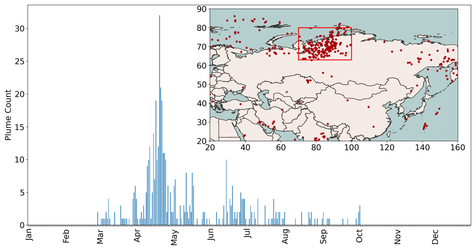
Figure 5 Number of plume detections per day for during 2023 within the red box on the inset map (centred over Norilsk, Russia).

Using the DBSCAN (Density-Based Spatial Clustering of Applications with Noise) algorithm (Ester et al., 1996), we grouped the detected plumes based on the coordinates of their maximum SO₂ observation (our proxy for origin). We set the clustering parameters to a maximum distance of 50 km between points and a minimum of 20 samples per cluster. This technique effectively identifies global areas with a high concentration of plumes. Figure 6 shows the centers of the 90 detected clusters, coloured by the number of plumes they contain, which further validates that our model successfully identifies the major SO₂ sources worldwide.

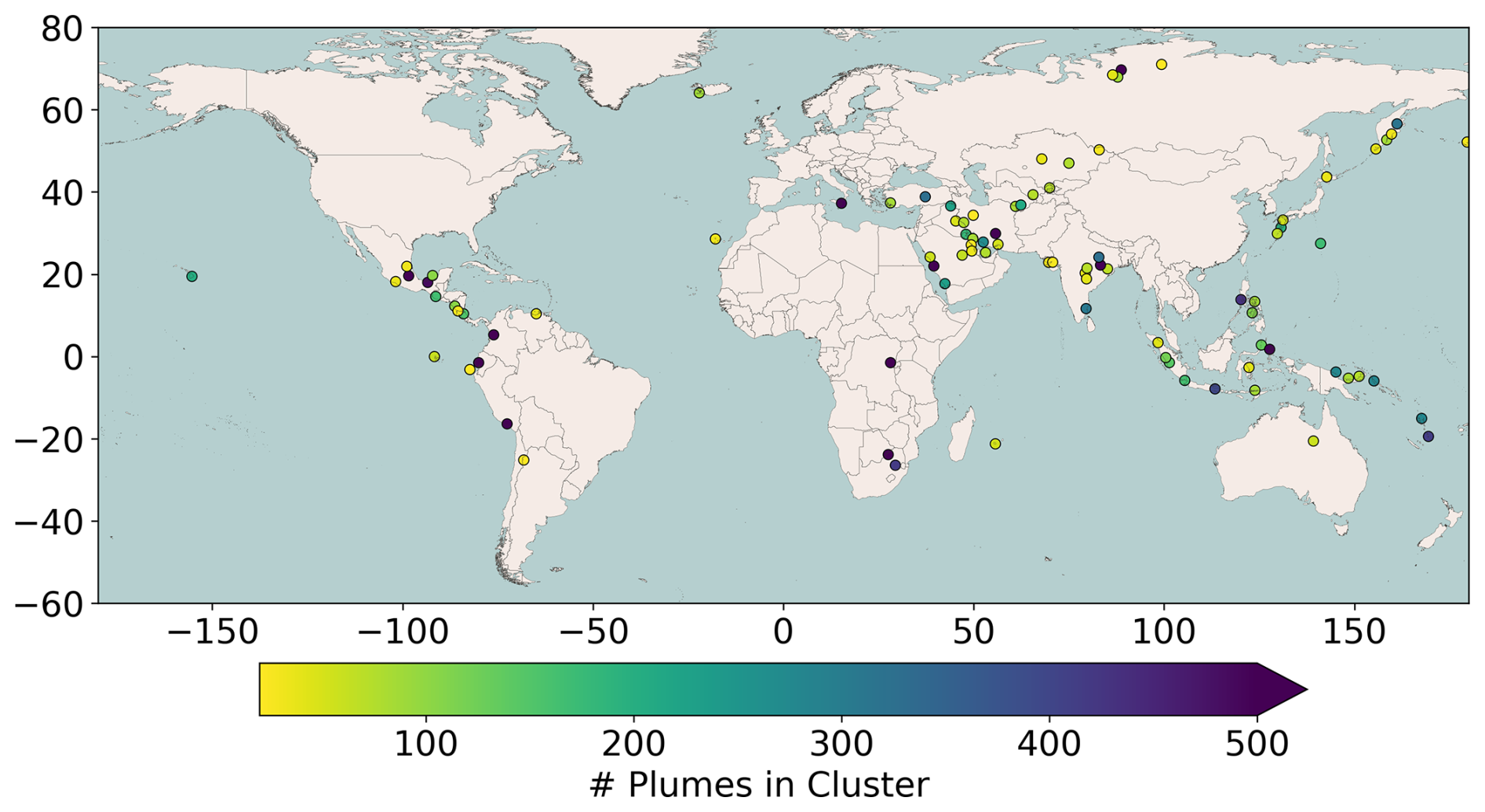
Figure 6 Locations of the centre of a cluster of plumes coloured by number of plumes in that cluster.

We observed regions on the global maps, most notably China (a location with numerous known SO₂ sources), where the model failed to detect expected plumes. Assuming the quality and volume of TROPOMI data are consistent globally, this deficiency likely stems from the plume detection model itself. We hypothesize that high background SO₂ concentrations in such regions may “hide” point sources, making plumes difficult to isolate. Although emissions of SO₂ have declined in China over the past couple of decades, ambient SO₂ levels are still relatively high compared to the rest of the globe (Wang et al., 2025), potentially making this effect more prominent in this region. Since the model was trained on global data, it may struggle with these outlier scenarios. Future iterations should address this by specifically training on data that includes plumes from high-background regions like China.

Table 2 Top ten largest clusters of plumes detected and their probable source, the total number of plumes over the 6 year study period, the median emission rate for all plumes in the cluster and the percentage of days a plume is detected in this region.

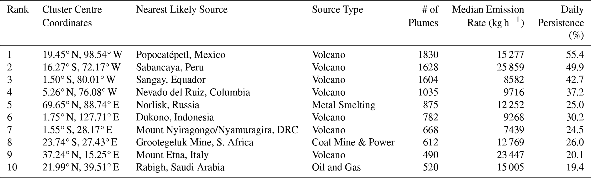
Table 2 details the ten largest clusters of SO₂ plumes detected over the 6-year study, alongside their probable sources. Volcanic activity dominates this list, accounting for seven out of the ten largest clusters. The remaining three clusters are associated with industrial activities: metal smelting, coal mining, and oil and gas operations. It is crucial to note that these clusters are often complex; some may contain multiple source types. For example, the Iztaccíhuatl volcano cluster is located just south of Mexico City, meaning the cluster likely includes industrial SO₂ sources alongside the volcanic emissions.

There is no notable impact on the plume detection results due to the increase in the across-track spatial resolution of the TROPOMI SO₂ product on 6 August 2019 from 7.0–5.5 km. There is larger variation in pixel size between the nadir and edge of swath observations than the increase in resolution and the model copes well with all these variations.

3.2 Coincidence with Volcanic Activity

Using the Smithsonian Institution's Global Volcanism Program (GVP) database of known eruptions since 1960 (GVP, 2026), we identified 227 active global eruptions during our study period. Comparing this list with our plume database revealed that 7943 plumes were detected within a 50 km radius of an eruption during its active date. This confirms plume detection for 110 (49 %) of these eruptions. The 117 missing detections are likely due to poor TROPOMI retrievals caused by high cloud cover or heavy aerosol loading. Figure 7 maps these GVP-reported eruptions, coloured by whether plumes were detected nearby (red) or not (green).

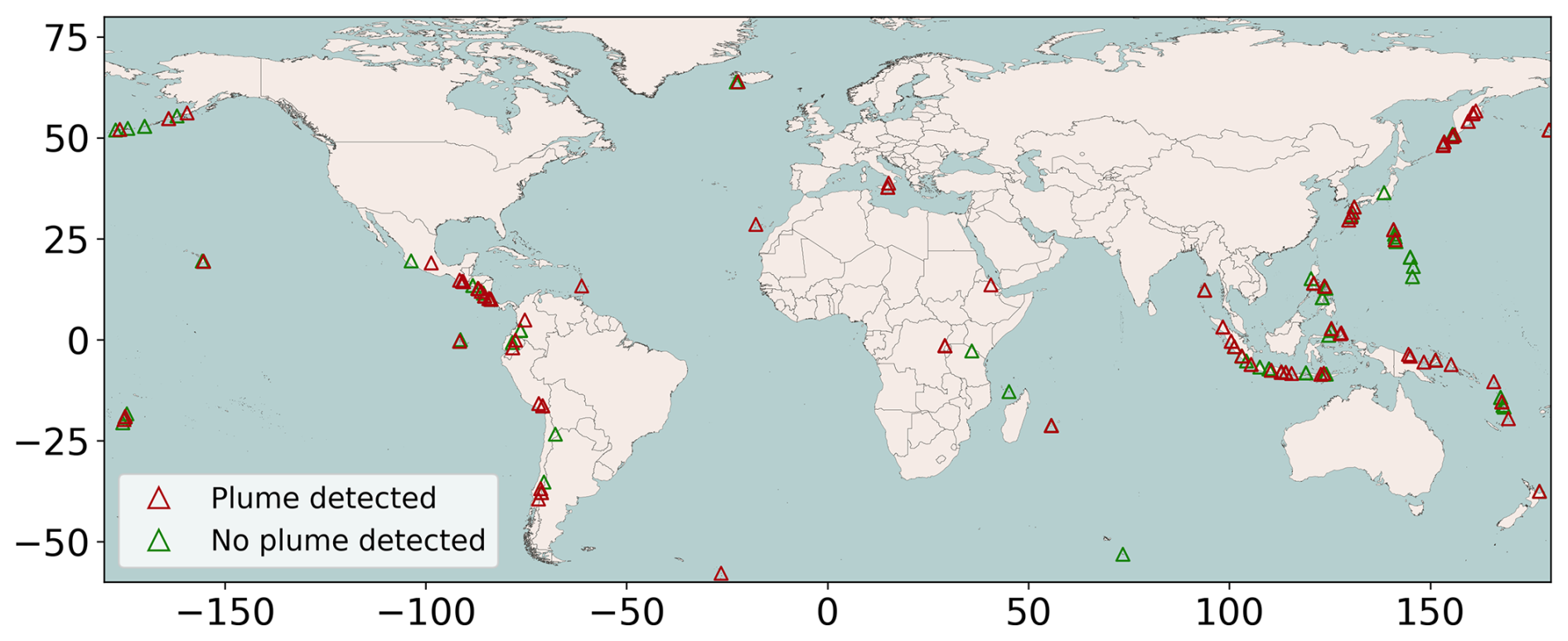
Figure 7 All eruptions reported between January 2019 and December 2024. Red triangles indicate plumes were detected within 50 km radius of the eruption during the eruptions dates. Green indicate no plume was detected.

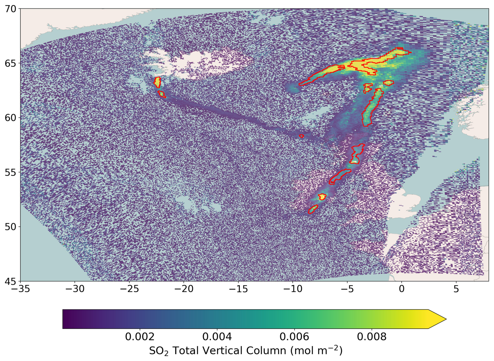
Figure 8 TROPOMI SO₂ total vertical column over the United Kingdom on 24 August 2024 showing a plume from the Svartsengi volcanic system in Iceland.

The plume detection algorithm struggles with very large plumes (> 1000 km) that often occur far downwind of major eruptions. Figure 8 illustrates this, showing a large SO₂ plume over the United Kingdom on 24 August 2024, originating from the Svartsengi volcanic system in Iceland (63.8° N, 22.38° W) six days earlier. The red outlines show the model splits this large plume into multiple smaller segments. This error likely results from the method used to break the TROPOMI swath into smaller images, which prevents the model from seeing the larger context of a plume that can span the entire swath.

3.3 TROPOMI SO₂ Activity Detection Flag

The TROPOMI Level 2 data assigns a flag to SO₂ pixels based on five categories: (0) no enhancement, (1) general SO₂ detection, (2) near a known volcano, (3) near a known anthropogenic source, and (4) a potential false positive due to a high solar zenith angle. Since a single plume often covers many pixels, we assign the final plume label only if over 80 % of its pixels share the same TROPOMI flag (likely determined by spatial proximity to known sources); otherwise, the plume is labeled as a combined source. We found that the dominant category is a general SO₂ detection with no source attribution (43.5 % of plumes), followed by volcanic plumes (30.8 %) and known anthropogenic sources (14.7 %). Figure 9 illustrates the geographical distribution of these categorized plumes.

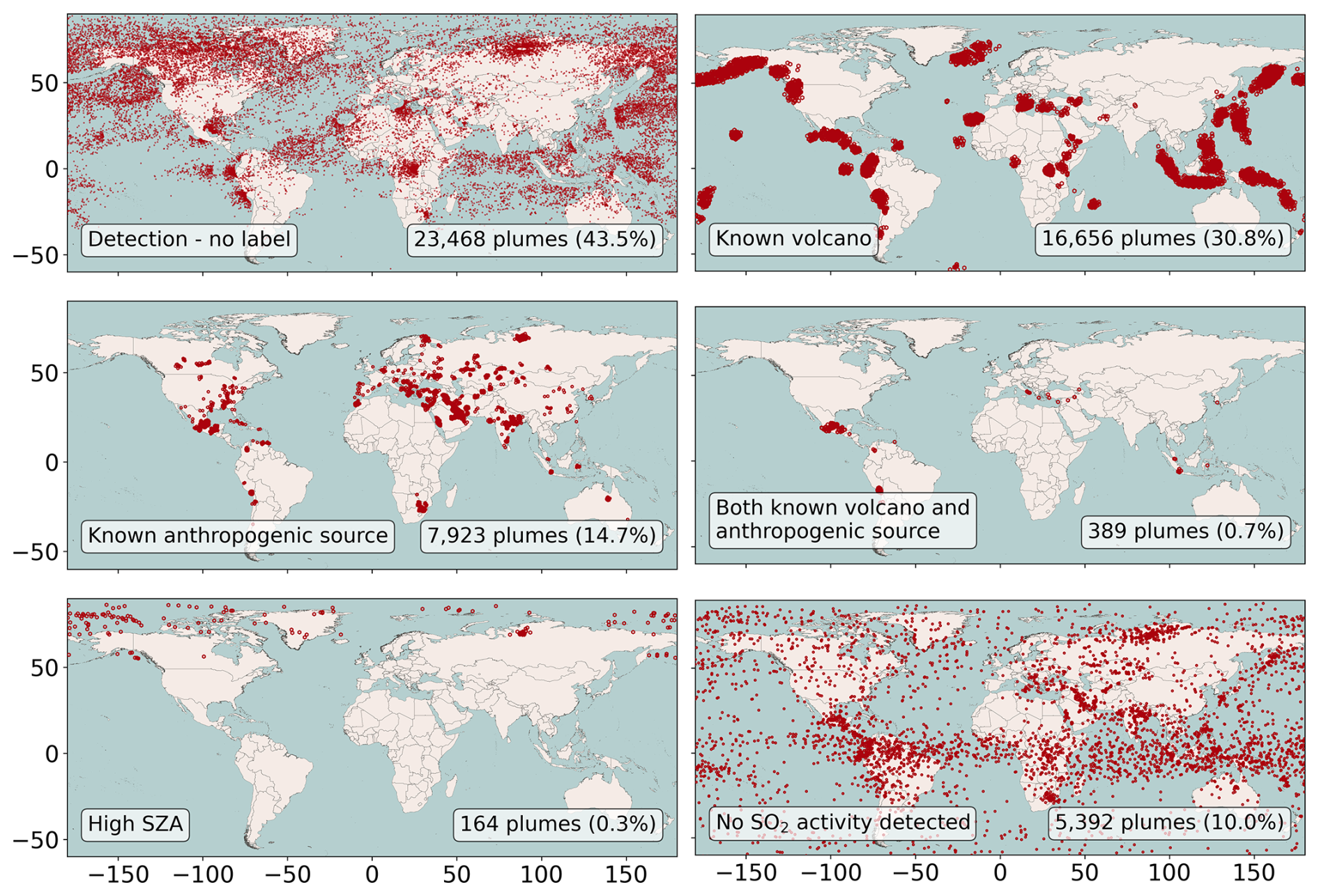
Figure 9 Global distribution of plume labels, 2019–2024, linked with the TROPOMI flag assigned to Level 2 SO₂ data.

The high number of unlabelled SO₂ detections is likely caused by plumes that have traveled downwind from their origin and are thus no longer close to the known volcanic or anthropogenic sources used for TROPOMI flagging. This explanation is strongly supported by the evidence of extensive volcanic outflow visible in both the geographical distribution of plumes (Fig. 3) and the daily detection spikes (Fig. 4).

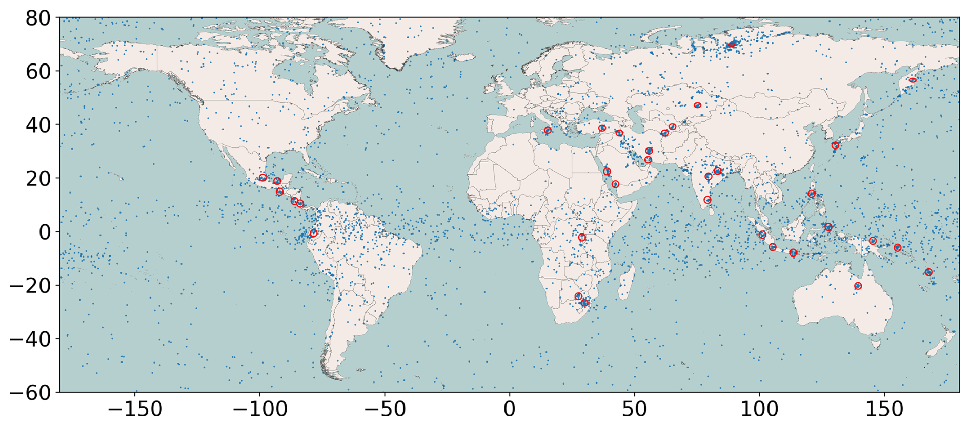
Figure 10 Location of all plumes labelled as “no enhanced detection” (blue), along with 34 clusters of more than 20 plumes within 150 km of each other (red) circles.

The TROPOMI “No enhanced SO₂ detected” category accounts for 10.0 % of all detections, but we believe many of these should be attributed to an actual source rather than being false positives. We demonstrate this by applying the clustering algorithm (as described in Sect. 3.1) to these “no enhanced detection” plumes. This allows us to extract meaningful groupings and calculate their proximity to clusters with known sources. Figure 10 displays all plumes in this category, highlighting 34 dense clusters (minimum 20 plumes within 150 km). Crucially, 27 of these 34 clusters overlap with clusters that have a known emission source, and the remaining seven are within 300 km. While these clusters account for 24 % of the “no enhanced detection” plumes, many of the remaining plumes form a large, dispersed swath extending from 100° E to 180 ° W around 10° S. This pattern aligns strongly with the downwind transport of SO₂ from the Taal Volcano eruption in the Philippines (120.99° E, 14.01° N) in April 2024 (detailed in Sect. 3.1).

This analysis demonstrates that while the source labelling provided in the TROPOMI files is informative, there is potential for our plume detection algorithm to complement the current flagging through masking and grouping plumes, facilitating analysis into repeated new detections. Although our plume detection algorithm does not attribute sources itself, it successfully highlights geographical and temporal patterns that are crucial for identifying important, and potentially unlabelled, SO₂ emission locations.

4 Concluding Remarks

The segmentation model successfully processed approximately 31 000 TROPOMI Level 2 files from 2019 to 2024, demonstrating scalability and efficiency, with a rapid processing time of about 15 s per swath on a GPU. The methodology, which employed a 32 × 32 pixel rolling window and median probability overlap, effectively addressed issues related to plumes straddling image boundaries while ensuring the final plume shape was not constrained by the input image size. Although the raw performance metrics (Precision: 65.7 %, Recall: 74 %) may appear modest, they are negatively skewed by the high sensitivity of using small 32 × 32 pixel images for validation. The model was deemed sufficient to establish a viable “first guess” emission database.

The global analysis confirmed that plumes cluster predictably around known volcanic and industrial hotspots. The detection of 53 993 plumes highlighted the critical role of episodic volcanic activity in SO₂ budgets, with significant annual spikes attributed to major events like the Raikoke and Ulawun eruptions in 2019. We also found that the TROPOMI Level 2 source flagging is incomplete; 43.5 % of detections were unlabelled, a finding we attribute to plumes being transported far downwind from their designated source areas. Clustering analysis of the “No enhanced SO₂ detected” plumes (10.0 % of detections) showed that many are, in fact, real sources, often corresponding to large, diluted outflow features like the plume from the 2024 Taal eruption.

However, two primary limitations must be addressed in future work. First, the algorithm struggles with very large plumes ($>\sim$ 1000 km), often incorrectly segmenting them into multiple smaller plumes due to the inherent context limitation of the small image input method. Second, and more critically, there is a pronounced lack of plume detection over expected high-emission industrial regions like China and India. We hypothesise that the algoirthm fails to isolate individual plumes against an excessively high SO₂ background concentration prevalent in these regions.

A crucial area for future advancement lies in integrating data from recently launched geostationary satellites. While the TROPOMI analysis relies on a single daily snapshot, instruments like the Geostationary Environment Monitoring Spectrometer (GEMS, covering Asia), the Tropospheric Emissions: Monitoring of Pollution (TEMPO, covering North America), and the future Sentinel-4 (covering Europe) offer sub-hourly or hourly measurements. This significantly higher temporal resolution would be transformative for this work, allowing for more robust plume tracking and improved wind field context for emission estimation. Furthermore, the hourly data would greatly enhance our ability to differentiate transient, high-flux plume events from persistent, high background SO₂ concentrations, thereby providing a pathway to potentially overcome the detection issues currently observed in heavily polluted industrial regions like China.

The application of machine learning is essential for achieving near real-time SO₂ source analysis, particularly for rapidly evolving natural hazards like volcanic eruptions. The immense processing speed of the segmentation model (sub-second per plume) is crucial for aviation safety, as SO₂ serves as a key proxy for hazardous volcanic ash. Machine learning automates the complex, time-consuming steps of plume boundary definition, geometric fitting (e.g., length), and emission rate calculation, transforming raw TROPOMI data into quantitative, actionable intelligence instantaneously. This rapid, objective assessment has the potential to inform Volcanic Ash Advisory Centers and provide timely input for atmospheric transport models, greatly enhancing warning systems and safety protocols.

Appendix A: Training Dataset Creation

To create the training dataset for the U-Net model, we followed the following steps:

• We first used an image classification model developed by Finch et al. (2022) for NO₂ plume to create a dataset of images possibly containing an SO₂ plume. Although the model was not developed for SO₂, we relied on the similar characteristics of NO₂ and SO₂ (e.g. point source emission and relativity short lifetime) to have a first pass at reducing the number of images to manually check. We put all available SO₂ swaths from 2019 and 2020 through the classification model for this first step.

• This first pass produced approximately 500 32 × 32 pixel images.

• We then developed a simple web application using Python and Plotly Dash (https://dash.plotly.com, last access: 14 March 2026) which loaded each of these images one by one for manual verification and to draw a boundary around the plume. The web application also provided a RGB satellite image of the same geographical area as the TROPOMI image to help the user determine if the plume was genuine or a likely false positive. A counter of the number of plumes verified was also provided. A screenshot of app is provided in Fig. A1.

• To draw the boundary around the plume, the user uses the mouse cursor to draw a line around what they believe is the plume boundary. This line is then saved and converted to both latitude and longitude coordinates and TROPOMI swath index coordinates and a plume mask is produced relating to the image.

• This process was repeated after numerous iterations of training and checking the plume detection model to refine the output.

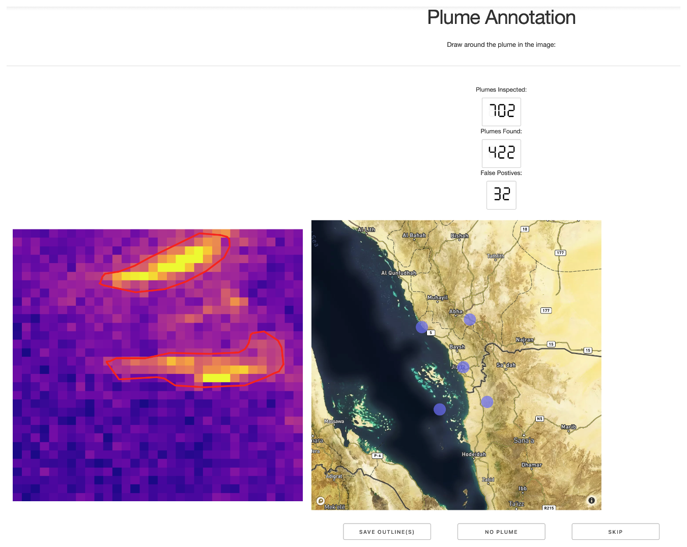
Figure A1 A screenshot of the plume annotation web app developed to draw boundaries around plumes of SO₂ in TROPOMI data. The image on the left shows the TROPOMI data and the image on the right shows a RGB image of the same ground location to use as a sanity check for the plume.

Appendix B: Major Volcanic Outflow

Figure B1 shows the plumes detected near likely volcanic eruptions, coloured by the days elapsed since the first eruption was detected. These show how these plumes are likely outflow from these large eruptions which are likely being detected on subsequent days as they are transported downwind.

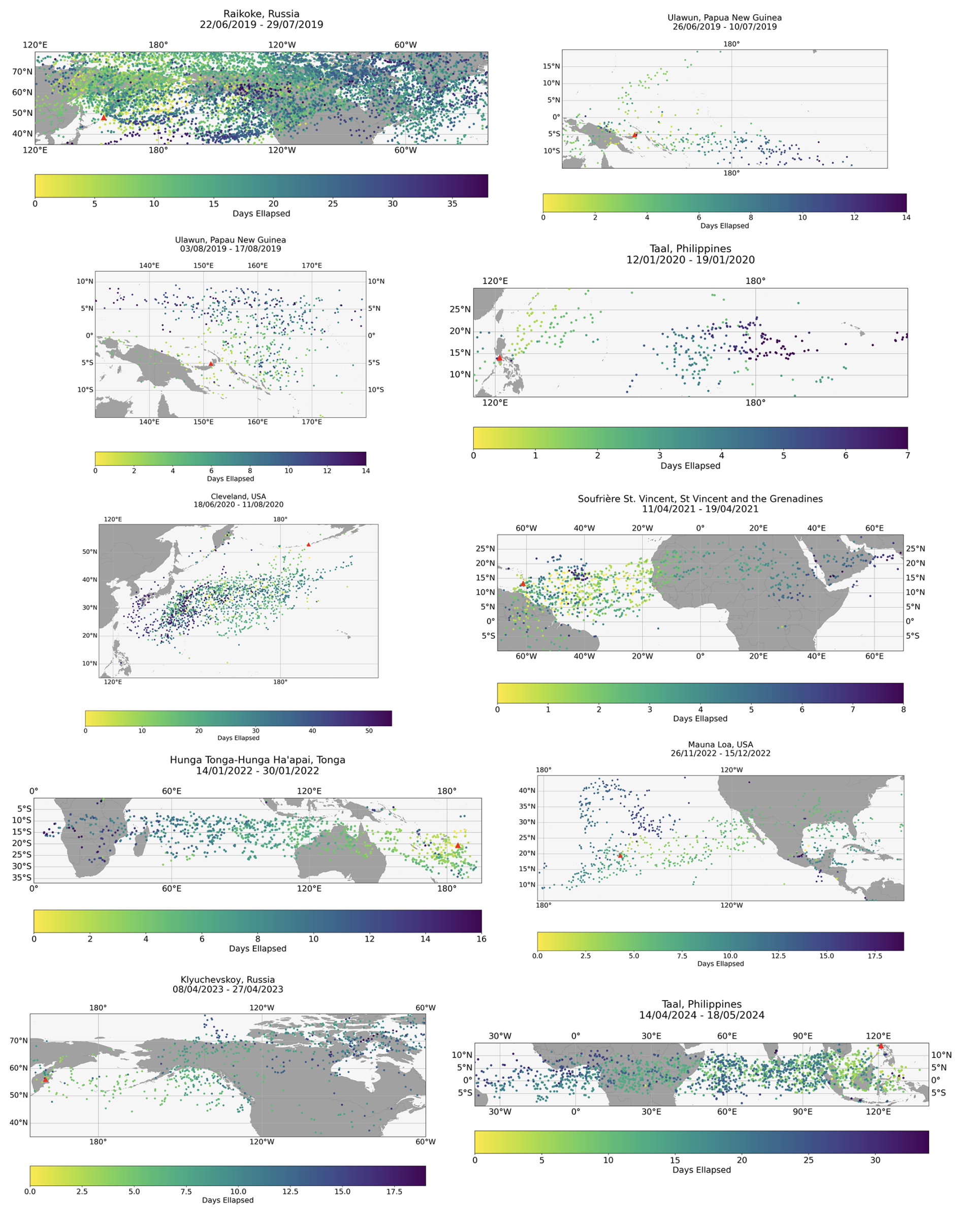
Figure B1 Plumes likely associated with major volcanic eruptions through the study period. The colouring represents days elapsed since first eruption detected.

Appendix C: Plume Dataset Description

The resulting plume dataset described in this paper is available for use and contains the following information:

• Date and time of the TROPOMI swath

• Latitude and longitude of the maximum SO₂ value within the plume (degrees north and west)

• X and Y Index on the TROPOMI swath of location of the maximum SO₂ value within the plume

• Value of the maximum SO₂ concentration within the plume (mol m⁻²)

• Indices on the TROPOMI swath of the bounding box surrounding the plume

• Plume mass enhancement from the background (kg)

• Latitude and longitudes of the plume border (degree north and west)

• Indices on the TROPOMI swath of the plume border

• Data on the fitted ellipse (x and y of ellipse centre, width, height and angle)

• Median, minimum, maximum, standard deviation and standard error of wind speed (m s⁻¹)

• Wind direction (degrees)

• Plume length (m)

• Plume emission estimate (kg h⁻¹)

• Array of pixel areas within the bounding box (m²)

• U and V wind fields within the bounding box

• Name of the original TROPOMI file used