Raman lidar-derived aerosol optical properties and classification during the FENNEC experiment – coherence with CAMS data

As part of the FENNEC programme, a field campaign was conducted on the Mediterranean coast of southern Spain, near Gibraltar, from June to August 2011. Using a straightforward ground-based N₂–Raman lidar, several aerosol optical properties were retrieved at 355 nm, including the linear particle depolarisation ratio (PDR), the lidar ratio (LR), and the aerosol backscatter and extinction coefficients. From continuous sampling over 58 nights, several periods were identified in which aerosol events exhibited optical thicknesses greater than 0.5. The primary drivers of these events are the incursions of Saharan dust mixed with local polluted and marine air masses. Pairing PDR and LR has been shown to be effective in identifying three distinct bulk aerosol classes: dust, carbonaceous and soluble (predominantly marine) aerosols. After processing the night-time data to ensure sufficient lidar range, the study demonstrates the effectiveness of lidar profiles in evaluating the reliability of the Copernicus Atmosphere Monitoring Service (CAMS) reanalyses of atmospheric aerosols up to approximately 7 km above mean sea level (a.m.s.l.). The two datasets show excellent consistency in terms of the optical thickness and vertical profile of the aerosol extinction coefficient in the Saharan dust aerosol layers. CAMS reproduces the temporal evolution well, with a correlation coefficient (COR) greater than 0.8. However, this is less accurate for the layer below 2 km a.m.s.l. (COR = 0.55), where CAMS tends to underestimate compared to ground-based lidar.

1 Introduction

Modelling is essential for characterising aerosol types and providing the most accurate possible assessment of their impacts on climate (Giorgi and Lionello, 2008; IPCC, 2022; Nabat et al., 2015; Flamant et al., 2015), as well as on meteorology and air quality (Wang et al., 2013, 2014a; Benedetti et al., 2009; Huneeus et al., 2012; Fourrié et al., 2019). This process relies on the validation of model-derived estimates against relevant observations. However, identifying aerosol types from observations remains a challenging and active area of research. In particular, the ability to characterise aerosols as a function of altitude and time is crucial not only for the validation of chemistry transport models but also for the interpretation and validation of spaceborne observations.

Significant progress on aerosol typing has been achieved with the advent of satellite missions carrying lidar instruments, such as the Cloud-Aerosol Lidar and Infrared Pathfinder Satellite Observations (CALIPSO) (Winker et al., 2009). This algorithm is based primarily on the use of aerosol depolarisation and spectral dependence (i.e. colour ratio) (Omar et al., 2009; Kim et al., 2018). Dedicated field campaigns were conducted both to support the development of the mission and to validate its products. These efforts notably relied on polarised and multispectral lidar measurements to discriminate between different aerosol types and their potential mixtures (Burton et al., 2012). The recent launch of the Earth Cloud, Aerosol and Radiation Explorer (EarthCARE) satellite mission (Wehr et al., 2023) has underscored the need for robust validation methods to accurately identify the different aerosol types. This need is particularly critical given that the mission relies solely on polarised channels at 355 nm in order to optimise the performance of the high-spectral-resolution atmospheric lidar (ATLID). Consequently, aerosol typing must primarily rely on the lidar ratio (LR) and the linear particle depolarisation ratio (PDR). Although the operational algorithm accounts for a range of aerosol types, significant overlaps between classes may still occur. Hence, based on end-to-end simulations of ATLID, the Hybrid End-to-End Aerosol Classification (HETEAC) was proposed (Wandinger et al., 2023; Holzer-Popp et al., 2013). Four basic aerosol components with prescribed microphysical properties are used to represent various natural and anthropogenic aerosols in the troposphere, representative of pollution, smoke, sea salt, and dust. Simultaneously, an approach based on an optimal estimation method (Rogers et al., 2009) has been implemented (Floutsi et al., 2024). This nonlinear regression scheme is applied to determine the statistically most likely atmospheric conditions and requires initialization with a priori information, as well as knowledge of the variance–covariance matrices of both the observables and the radiative transfer model (i.e., the lidar simulator).

This study presents an approach based on a straightforward N₂–Raman lidar technique for retrieving aerosol optical properties at 355 nm with high spatial resolution in the troposphere, for the purpose of performing aerosol classification. It should be noted that Raman lidar observations have previously been used in conjunction with measurements at two wavelengths (532 and 1064 nm) to identify four aerosol classes (Nishizawa et al., 2017). The study examines the temporal evolution of these properties during the FENNEC (https://africanclimateoxford.net/projects/fennec/, last access: 4 April 2026) ground-based field campaign conducted from mid-June to the end of August 2011. The focus is on identifying different types of aerosols (e.g. dust, carbonaceous, and soluble particles). The resulting optical apportionment (i.e. the classification of aerosols using optical measurements) is then compared with mesoscale simulations of the chemical composition of aerosols from the Copernicus Atmosphere Monitoring Service (CAMS; https://atmosphere.copernicus.eu/, last access: 8 February 2026) (Inness et al., 2019). This is performed alongside a study comparing the optical properties of aerosols (i.e. aerosol optical thickness and vertical profiles of the aerosol extinction coefficient) retrieved from Raman lidar measurements with those derived from numerical simulations. Unlike spaceborne lidar observations, for which few coincidences are available due to satellite revisits, this method provides a substantial amount of statistical overlap during the field campaign. Consequently, the reliability of the CAMS reanalysis of aerosols can be examined to enhance our understanding of the impact of aerosols on climate and air quality. However, this is also part of the long-term vision to use modelling data alongside ATLID products.

2 Experimental set up and tools

2.1 FENNEC field campaign

The FENNEC airborne component took place from June to July 2011 (Ryder et al., 2015; Marsham et al., 2013), and was extended to include ground-based measurements from 25 June to 23 August. These measurements primarily focused on the contribution of Saharan dust to the atmospheric particle load. During this extended summer period, the vertical distribution of aerosols was monitored from a ground-based remote sensing station located in San Pedro Alcántara, southern Spain (36°29^′11^′′ N, 4° 59^′33^′′ W), between Gibraltar and Marbella in Andalusia (Fig. 1a). The complex topography of the Mediterranean coastline at this site gives rise to contrasting air masses in the lower and middle troposphere (Rodríguez et al., 2001). These air masses transport a variety of aerosol types, whose physicochemical and optical properties are closely linked to their source regions (e.g. the Sahara area).

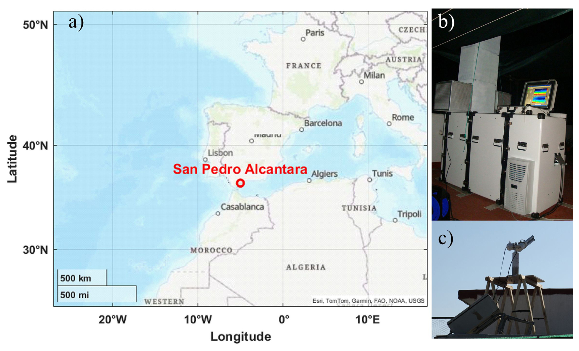
Figure 1 (a) Location of the ground-based station (in red) where (b) the LAASURS lidar and (c) the sun photometer were installed. Sources: Esri, TomTom, FAO, USGS | Powered by Esri.

The FENNEC ground-based experiment follows the Mediterranean Dust Experiment (MEDUSE) (Hamonou et al., 1999; Dulac and Chazette, 2003) and predates the Chemistry-Aerosol Mediterranean Experiment (ChArMEx), which was conducted between 2013 and 2014 (Chazette et al., 2016b; Di Girolamo et al., 2020; Chazette et al., 2019; Mallet et al., 2016). The latter notably included contributions from the European Aerosol Research Lidar Network (EARLINET) (Barragan et al., 2017; Navas-Guzmán et al., 2013). Compared with these campaigns, FENNEC provided an exceptionally long and continuous lidar sampling of the troposphere in cloud-free troposphere.

2.2 Ground-based observations

2.2.1 Site description

Continuous optical measurements were performed during the field campaign. The seaside location was chosen because of the potential to experience: (i) strong events of particle transport from the Sahara, (ii) presence of pollution or biomass fire plumes, and (iii) high variability in aerosol optical thickness (AOT) (Rodríguez et al., 2001; Toledano et al., 2007). Located at an altitude of 110 m above mean sea level (a.m.s.l.), the station offered a 360° panoramic view.

2.2.2 Ground-based Raman lidar

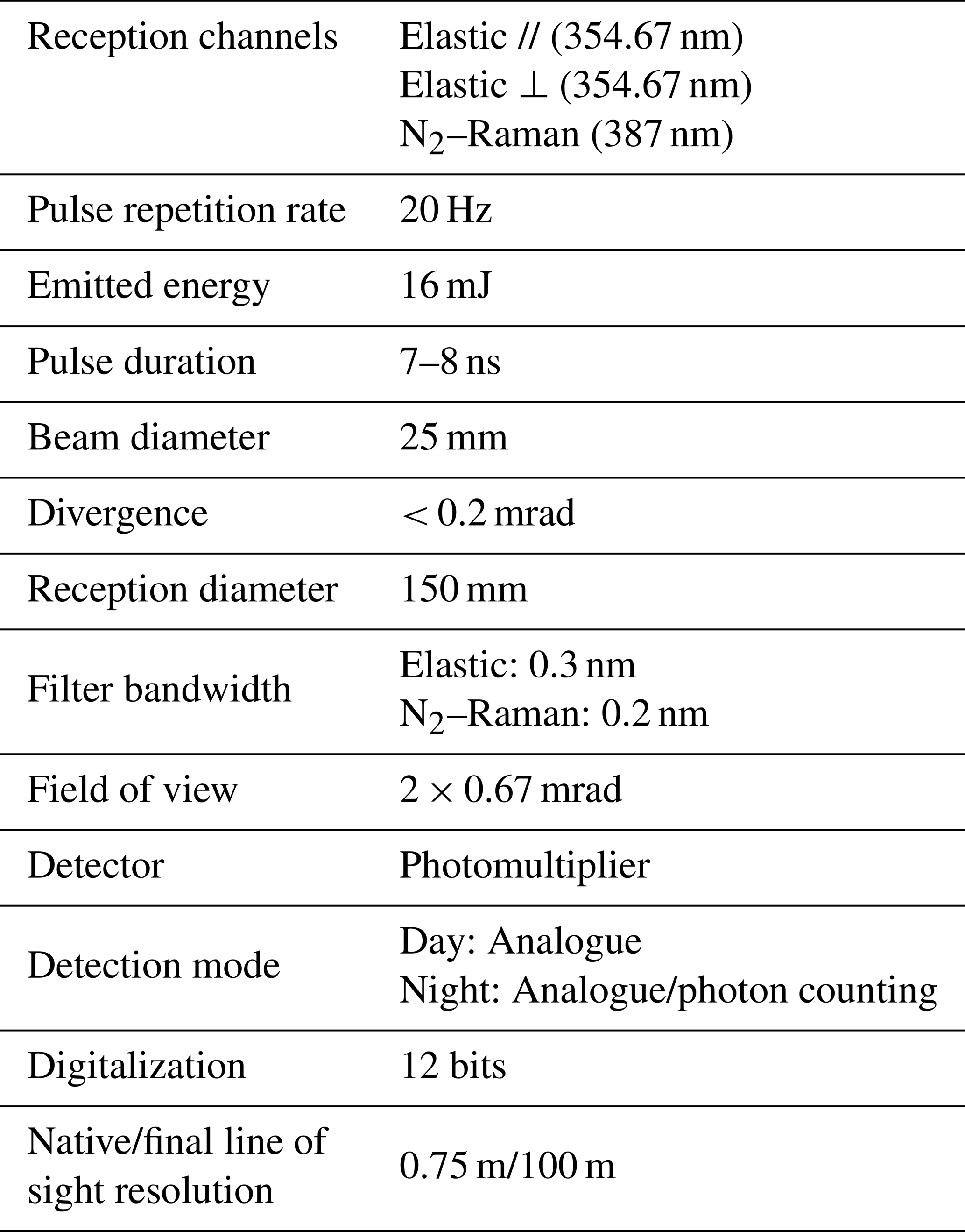
LAASURS (Lidar for Automatic Atmospheric Surveys using Raman Scattering) is the precursor to the Water vapour and Aerosol LIdar (WALI), which was used in a series of Mediterranean field experiments (Chazette et al., 2016a, 2014). LAASURS (Fig. 1b) itself is described in detail and validated in Royer et al. (2011a) and Chazette et al. (2019). It has been used in numerous field campaigns, such as the journey from Paris to Lake Baikal (Dieudonné et al., 2015). LAASURS is a French lidar system that remains operational and uses proven technology that has also been employed in recent research activities (Laly et al., 2024). The main characteristics of LAASURS are given in Table 1. Its wide field-of-view (FOV) of ∼ 2.3 mrad enables full overlap of the transmission and reception paths at distances of ∼ 200 m. Three different channels record (i) the total elastic backscatter signal of the atmosphere (elastic channels), (ii) the cross-polarised elastic backscatter signal of the atmosphere with respect to the laser emission, and (iii) the inelastic nitrogen vibrational Raman backscattered signal (N₂–Raman channel). Using the N₂–Raman channel at night allows the cumulative AOT profiles to be retrieved. When this is combined with the elastic channel, the lidar ratio (LR) is derived (e.g. Royer et al., 2011a).

Table 1 Main characteristics of LAASURS.

The lidar measured atmospheric properties with a temporal native resolution of approximately 50 s, i.e. an average of 1000 elementary profiles, and a vertical resolution of 0.75 m. In order to pass through desert aerosol layers, which can reach heights of over 7 km, it is necessary to reduce the temporal and vertical resolutions. The profiles are averaged over nights, with the vertical resolution reduced to 100 m, in order to improve the signal-to-noise ratio (SNR) and enable access to the upper troposphere (see Sect. 3).

2.2.3 Sun photometer

A sun photometer (Fig. 1c) was installed at the temporary lidar site during the experiment to provide additional measurements alongside those obtained by lidar. This study takes into consideration both ultraviolet and visible optical thicknesses. These are then combined with the Ångström exponent, which was calculated between 380 and 500 nm, to determine the AOT at 355 nm during the daytime. Sun photometer data were derived from the temporary station of the AErosol RObotic NETwork (AERONET) in San Pedro Alcantara (http://aeronet.gsfc.nasa.gov/, last access: 24 January 2026). Level 2 data, which has undergone cloud screening (Dubovik and King, 2000), are used. The AOT is retrieved with a maximum absolute uncertainty of 0.02, independent of the aerosol load.

2.3 CAMS

CAMS global reanalysis (EAC4) has a horizontal resolution of 0.75° × 0.75° and is provided by the Copernicus Atmosphere Monitoring Service (CAMS, https://atmosphere.copernicus.eu/, last access: 24 January 2026) (Inness et al., 2019). This study analyses the consistency of EAC4 with the optical apportionment of aerosols derived from LAASUR's vertical profiles. CAMS combines model data with various observations from across the world. In particular, AOTs derived from satellite observations, such as those of the Moderate Resolution Imaging Spectroradiometer (MODIS) (Remer et al., 2005), are directly assimilated into the model. Ground-based measurements from permanent AERONET stations are also used as a validation dataset. However, vertical aerosol profiles are not assimilated and are rarely considered for validation purposes. CAMS provides data on aerosol compounds: desert dust, sea salt, organic matter, black carbon, sulphate ions. In the following, soot and organic carbons are grouped together as “carbonaceous” aerosols, while ionic concentrations and sea salt are grouped together as “soluble” aerosols. It should be noted that the primary source of the latter aerosol types is marine for the site under consideration. As indicated by the findings of the research, dust, when present above the lidar station, serves as an indicator of the transport of Saharan aerosols. Carbonaceous aerosols, meanwhile, serve as an indicator of combustion (e.g. from traffic, industry, and forest fires). Finally, soluble aerosols serve mainly as an indicator of marine origins.

3 Method

3.1 Lidar-derived aerosol optical properties

During daylight hours, the range of the lidar is insufficient to determine the aerosol extinction coefficient (AEC), lidar ratio (LR) and linear particle depolarisation ratio (PDR) simultaneously. In order to ascertain the nature of the aerosols, i.e. whether they are dust-like, sea salt or polluted aerosols, it is necessary to evaluate these three optical parameters (Chazette et al., 2016a). This means collecting data at night and averaging it over a 6 h period, between 23:00 local time (LT) the previous day and 05:00 LT the following day. The SNR (SNR 10) is sufficient for inverting mean lidar profiles up to 8 km a.m.s.l., with an altitude zone between 7 and 8 km a.m.s.l. in which molecular scattering accounts for over 99 % of the total extinction. The mean lidar profiles thus exhibit a molecular slope between 7 and 8 km a.m.s.l., as illustrated in Fig. 2. The procedure used to invert the lidar profiles considers all LAASURS channels.

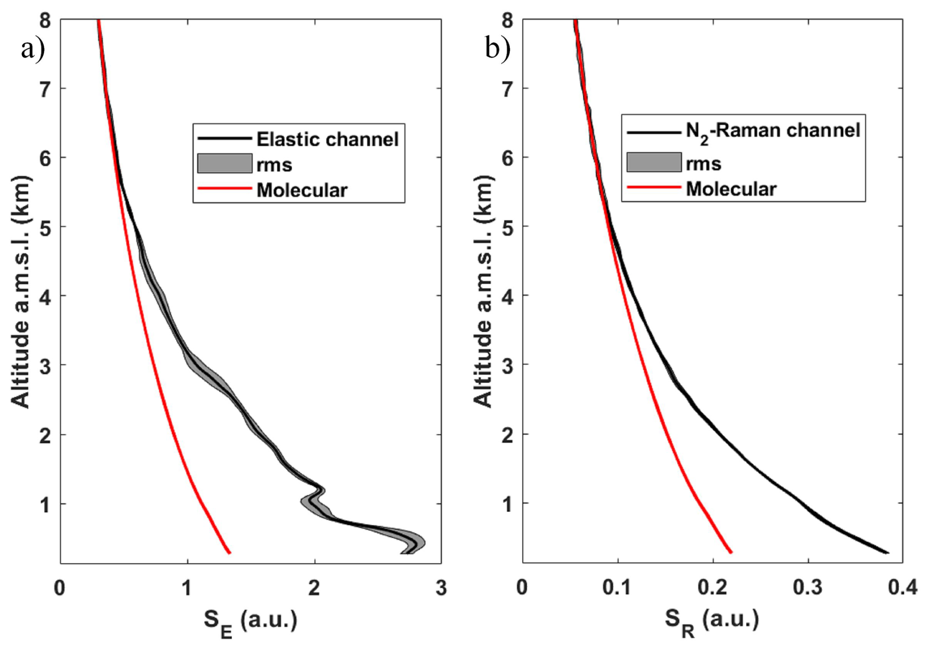
Figure 2 The mean vertical profiles of the range-corrected (a) elastic (S_E) and (b) Raman (S_R) channels are shown for the night of 27–28 June 2011, from 23:00 to 05:00 LT. The grey area shows the standard deviation of the mean vertical profiles. The red solid line indicates the molecular contribution.

The range-corrected elastic lidar signal S_E is expressed as a function of altitude z (e.g. Measures, 1984; Ansmann et al., 1992)

$$\begin{array}{}\text{(1)}& \begin{array}{rl}{S}_{\mathrm{E}}\left(z\right)& =C_{\mathrm{E}}\cdot \left({\mathit{\beta }}_{\mathrm{m}}\left(z\right)+{\mathit{\beta }}_{\mathrm{a}}\left(z\right)\right)\cdot F_{\mathrm{E}}\left(z\right)\\ & \cdot \exp \left[-\mathrm{2}\cdot \left({\mathit{\tau }}_{\mathrm{m}}\left(z\right)+{\mathit{\tau }}_{\mathrm{a}}\left(z\right)\right)\right]\end{array}\end{array}$$

The instrumental constant C_E of the elastic channel is independent of altitude, while the overlap function F_E tends towards 1 from 200 m (Royer et al., 2011b). The molecular (β_m) and particular (β_a) backscatter coefficients are provided for an emitted wavelength of 354.67 nm. The atmospheric attenuation is characterised by the molecular optical thickness (MOT) τ_m and the AOT τ_a.

For the N₂–Raman channel, the range-corrected lidar signal is given by (e.g. Royer et al., 2011a)

$$\begin{array}{}\text{(2)}& \begin{array}{rl}{S}_{\mathrm{R}}\left(z\right)& =C_{\mathrm{R}}\cdot F_{\mathrm{R}}\left(z\right)\cdot N_{\mathrm{m}}\left(z\right)\\ & \cdot \exp \left[-\left(\mathrm{1}+{\mathit{\eta }}_{\mathrm{m}}\right)\cdot {\mathit{\tau }}_{\mathrm{m}}\left(z\right)-\left(\mathrm{1}+{\mathit{\eta }}_{\mathrm{a}}\right)\cdot {\mathit{\tau }}_{\mathrm{a}}\left(z\right)\right]\end{array}\end{array}$$

with

$$\begin{array}{}\text{(3)}& \begin{array}{l}{\mathit{\eta }}_{\mathrm{m}}={\left(\frac{\mathrm{387}}{\mathrm{354.67}}\right)}^{-\mathrm{4.09}}\\ {\mathit{\eta }}_{\mathrm{a}}={\left(\frac{\mathrm{387}}{\mathrm{354.67}}\right)}^{-A}\end{array}\end{array}$$

The instrumental constant of the inelastic channel system is C_R, and the overlap function is F_R. In this equation, the Ångström exponent A must be considered. Here, A has been derived from the interpolation of the sun photometer measurements (Fig. 3). By normalising Eq. (3) to a reference altitude z₀ located at the bottom of the profile, where the overlap functions are well-defined (for example, when it tends towards 1), the AOT between z₀ and z can be expressed as follows:

$$\begin{array}{}\text{(4)}& \begin{array}{rl}{\mathit{\tau }}_{\mathrm{a}}\left(z_{\mathrm{0}},z\right)={\displaystyle \frac{\mathrm{1}}{\mathrm{1}+{\mathit{\eta }}_{\mathrm{a}}}}\cdot [& \log \left({\displaystyle \frac{N_{\mathrm{m}}\left(z\right)}{N_m\left(z_{\mathrm{0}}\right)}}\cdot {\displaystyle \frac{S_{\mathrm{R}}\left(z_{\mathrm{0}}\right)}{S_{\mathrm{R}}\left(z\right)}}\right)\\ & -\left(\mathrm{1}+{\mathit{\eta }}_{\mathrm{m}}\right)\cdot {\mathit{\tau }}_{\mathrm{m}}\left(z_{\mathrm{0},z}\right)]\end{array}\end{array}$$

This assumes a constant spectral variation of aerosol optical properties with altitude. The molecular contribution is calculated using the Nicolet (1984) model. The ERA5 reanalyses (Hersbach et al., 2020) from the European Centre for Medium-Range Weather Forecasts (ECMWF) are used as input data. These have been given for the geographical location of the lidar. The AEC (α_a) can then be calculated using a derivative low-pass filter of AOT with respect to z, as described by Dieudonné et al. (2015):

$$\begin{array}{}\text{(5)}& {\mathit{\alpha }}_{\mathrm{a}}\left(z_{\mathrm{0}},z\right)={\displaystyle \frac{\partial {\mathit{\tau }}_{\mathrm{a}}\left(z_{\mathrm{0}},z\right)}{\partial z}}\end{array}$$

For SNRs greater than 10, the margin of error is between 0.01 and 0.02 km⁻¹, which is larger at higher altitudes.

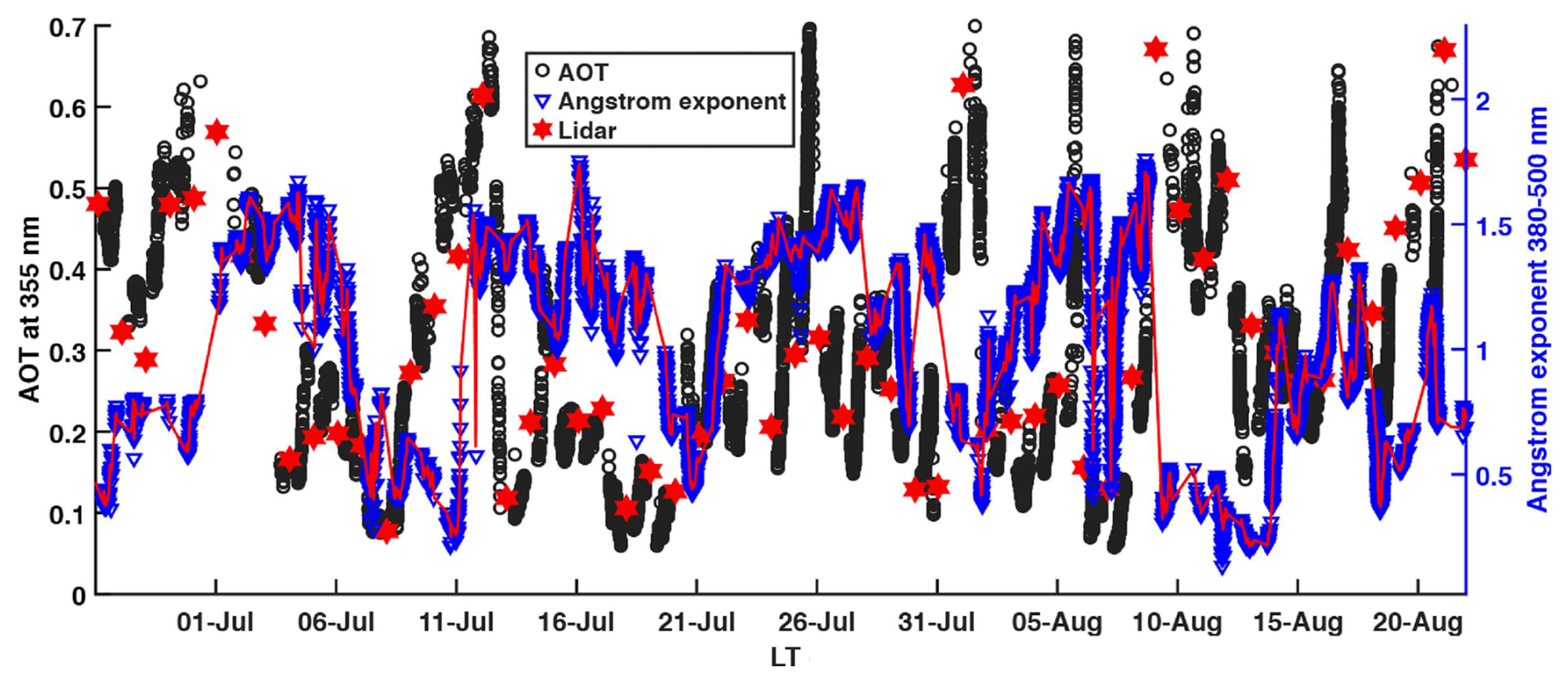
Figure 3 Temporal evolution of the sun photometer-derived aerosol optical thickness (AOT) at 355 nm and the Ångström exponent between 380 and 500 nm. The red solid line shows the interpolation used for the lidar profile inversion at night. The red star shows the lidar-derived AOT at night, from 23:00 to 05:00.

In Eq. (1), the atmospheric transmission must be corrected to calculate β_a. In order to maintain the correction at second order in terms of uncertainty, it is preferable to consider the ratio between the elastic and inelastic channels. In the molecular zone between 7 and 8 km a.m.s.l., this ratio can be evaluated using the relationship:

$$\begin{array}{}\text{(6)}& {\displaystyle \frac{C_{\mathrm{E}}}{C_{\mathrm{R}}}}=<{\displaystyle \frac{S_{\mathrm{E}}\left(z\right)}{S_{\mathrm{R}}\left(z\right)}}\cdot \exp \left[\left(\mathrm{1}-{\mathit{\eta }}_{\mathrm{m}}\right)\cdot {\mathit{\tau }}_{\mathrm{m}}\left(z\right)\right]{>}_{\mathrm{mol}}\end{array}$$

This method has been demonstrated to be efficient for calibrating lidar measurements in clear-sky conditions. The calculation is performed by averaging over the molecular altitude range (〈 〉_mol). For all altitudes z, β_a is then given by the same channel ratio:

$$\begin{array}{}\text{(7)}& \begin{array}{rl}{\mathit{\beta }}_{\mathrm{a}}\left(z\right)=(& {\displaystyle \frac{C_{\mathrm{R}}}{C_{\mathrm{E}}}}\cdot {\displaystyle \frac{S_{\mathrm{E}}\left(z\right)}{S_{\mathrm{R}}\left(z\right)}}\cdot \exp \left[\left(\mathrm{1}-{\mathit{\eta }}_{\mathrm{m}}\right)\cdot {\mathit{\tau }}_{\mathrm{m}}\left(z\right)\right]\\ & \cdot \exp \left[\left(\mathrm{1}-{\mathit{\eta }}_{\mathrm{a}}\right)\cdot {\mathit{\tau }}_{\mathrm{a}}\left(z\right)\right]-\mathrm{1})\cdot {\mathit{\beta }}_{\mathrm{m}}(z)\end{array}\end{array}$$

The extinction-to-backscatter ratio (Lidar Ratio, LR) L_r is subsequently determined by the following formula, which is dependent upon altitude:

$$\begin{array}{}\text{(8)}& L_{\mathrm{r}}\left(z\right)={\displaystyle \frac{{\mathit{\alpha }}_{\mathrm{a}}\left(z\right)}{{\mathit{\beta }}_{\mathrm{a}}\left(z\right)}}\end{array}$$

Royer et al. (2011a) used a Monte Carlo approach based on a Tikhonov regularisation method (Tikhonov and Arsenin, 1978) to show that the relative error in LR is less than 5 % at night for AOT greater than 0.2.

The final optical parameter to be deduced is the PDR δ_a, which is expressed as follows (Chazette et al., 2012):

$$\begin{array}{}\text{(9)}& {\mathit{\delta }}_{\mathrm{a}}\left(z\right)={\displaystyle \frac{{\mathit{\beta }}_{\mathrm{m}}\left(z\right)\cdot \left({\mathit{\delta }}_{\mathrm{vm}}-{\mathit{\delta }}_{\mathrm{v}}\left(z\right)\right)-{\mathit{\beta }}_{\mathrm{a}}\left(z\right)\cdot {\mathit{\delta }}_{\mathrm{v}}\left(z\right)\cdot \left(\mathrm{1}+{\mathit{\delta }}_{\mathrm{vm}}\right)}{{\mathit{\beta }}_{\mathrm{m}}\left(z\right)\cdot \left({\mathit{\delta }}_{\mathrm{v}}\left(z\right)-{\mathit{\delta }}_{\mathrm{vm}}\right)-{\mathit{\beta }}_{\mathrm{a}}\left(z\right)\cdot \left(\mathrm{1}+{\mathit{\delta }}_{\mathrm{vm}}\right)}}\end{array}$$

In accordance with Collis and Russel (1976), the molecular volume depolarization ratio (δ_vm) is taken to be 0.3945 % at 355 nm. The VDR δ_v is calculated according to the method described by Chazette et al. (2012). The PDR absolute uncertainties range from 1 % to 2 % for the encountered AOTs at 355 nm (AOT > 0.2) (Dieudonné et al., 2017).

3.2 CAMS-derived Aerosol optical properties

3.2.1 CAMS-derive aerosol extinction coefficient

The AEC at 550 nm can be assessed based on the mixing ratios, with the CAMS-derived AOT serving as a constraint. In the reanalysis, the AOTs take relative humidity (RH) into account, but this is based on several assumptions. The main assumptions are that aerosols do not change bin during growth with RH, and that for highly hydrophilic sea salt aerosols, only RH = 80 % is considered for both the AOT and mixing ratio (see https://www.ecmwf.int/sites/default/files/elibrary/112024/81 630-ifs-documentation-cy49r1-part-viii-atmospheric-composition.pdf, last access: 22 Jule 2026).

The wet AOT (τ_aW) should be calculated against the AEC (α_CAMS) at each altitude z using an equation of the form:

$$\begin{array}{}\text{(10)}& {\mathit{\tau }}_{\mathrm{aW}}\left(z\right)={\int }_{\mathrm{ground}}^z{\mathit{\alpha }}_{\mathrm{CAMS}}\left(z^{\prime }\right)\cdot \mathrm{d}{z}^{\prime }\end{array}$$

where considering each compound i:

$$\begin{array}{}\text{(11)}& {\mathit{\alpha }}_{\mathrm{CAMS}}\left(z\right)={\sum }_{i=\mathrm{1}}^{\mathrm{3}}{M}_{\mathrm{w}i}\left(z\right)\cdot {\mathit{\sigma }}_{\mathrm{W}i}\left(z\right)\end{array}$$

M_Wi and σ_Wi are the wet matter mass and the wet specific cross-section, respectively. Following Hänel (1976), M_Wi is a function of the dry matter mass, the mass increase coefficient μ_i and RH:

$$\begin{array}{}\text{(12)}& M_{\mathrm{W}i}\left(z\right)=M_{\mathrm{D}i}\left(z\right)\cdot \left(\mathrm{1}+{\mathit{\mu }}_i\left(z\right)\cdot {\displaystyle \frac{R_{\mathrm{H}}\left(z\right)}{(\mathrm{1}-R_{\mathrm{H}}(z\left)\right)}}\right)\end{array}$$

When hydrophilic aerosols are present in high concentrations in the model (below ∼ 1 km a.m.s.l.), the RH (R_H) remains stable at altitude with a certain degree of repetition from one night to the next in the lower layers. Values between 50 % and 80 % are observed (Fig. 4). This therefore reduces the impact of RH variability on calculations. Please note that below the deliquescence point, for RH between 50 % and 70 %, even 76.8 % for sea salt (McMurry and Stolzenburg, 1989; Randriamiarisoa et al., 2006), the hygroscopicity effect is low. It is therefore assumed here that product ${\mathit{\sigma }}_{\mathrm{W}i}\left(z\right)\cdot \left(\mathrm{1}+{\mathit{\mu }}_i\left(z\right)\cdot \frac{R_{\mathrm{H}}\left(z\right)}{(\mathrm{1}-R_{\mathrm{H}}(z\left)\right)}\right)$ remains constant for each type of aerosol. Therefore, the specific cross sections and the AEC can be evaluated using the mixture ratios r_i of each compound i (i.e. dust, carbonaceous matter and soluble matter) provided by CAMS, with the CAMS-derived AOTs at 550 nm serving as a constraint. It should be noted that the model assimilated spaceborne-derived AOTs and is validated using ground-based AOTs. The vertical profiles derived from the model are therefore adjusted accordingly. The AEC is then expressed according to the relationship:

$$\begin{array}{}\text{(13)}& {\mathit{\alpha }}_{\mathrm{CAMS}}\left(z\right)={\displaystyle \frac{M_{\mathrm{a}}}{N}}\cdot n_{\mathrm{a}}\left(z\right)\cdot {\sum }_{i=\mathrm{1}}^{\mathrm{3}}{r}_i\left(z\right)\cdot {\mathit{\sigma }}_{\mathrm{W}i}\end{array}$$

where M_a is the molar mass of dry air (28.94 g), N is Avogadro's number (6.022 × 10²³) and n_a is the atmospheric density. The values determined for the specific cross sections are given in Table 2. It should be noted that this wet specific cross-sectional is in fact a pseudo-specific cross-sectional.

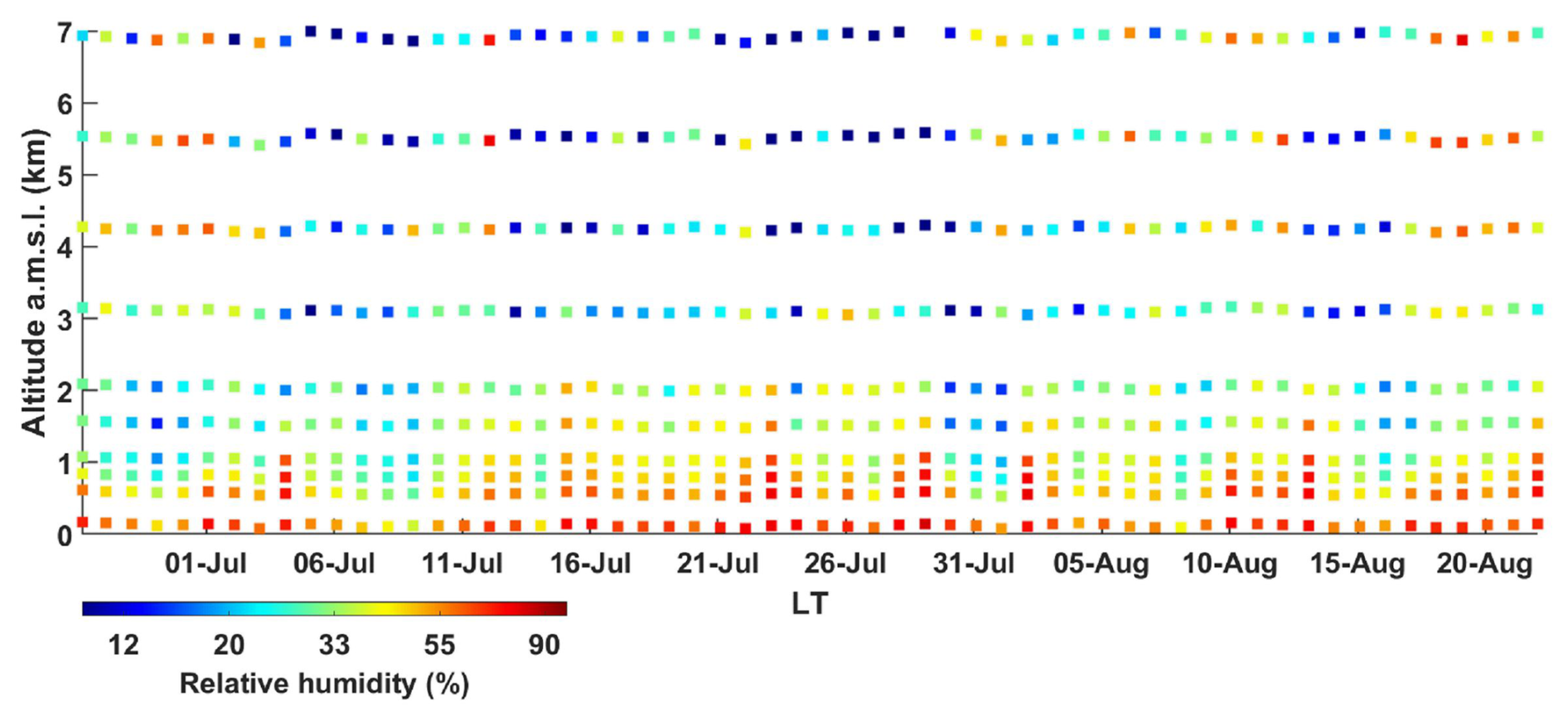
Figure 4 Temporal evolution of the mean values of the CAMS-derived relative humidity displayed for the period between 23:00 and 05:00 LT on a nightly basis.

Table 2 Specific cross sections σ_W assessed for each aerosol compound using the CAMS data. The statistical parameters of the comparison between the aerosol optical thicknesses (AOT) provided by CAMS and those recalculated are also given: mean bias (MB), root mean square error (RMSE) and corelation coefficient (COR).

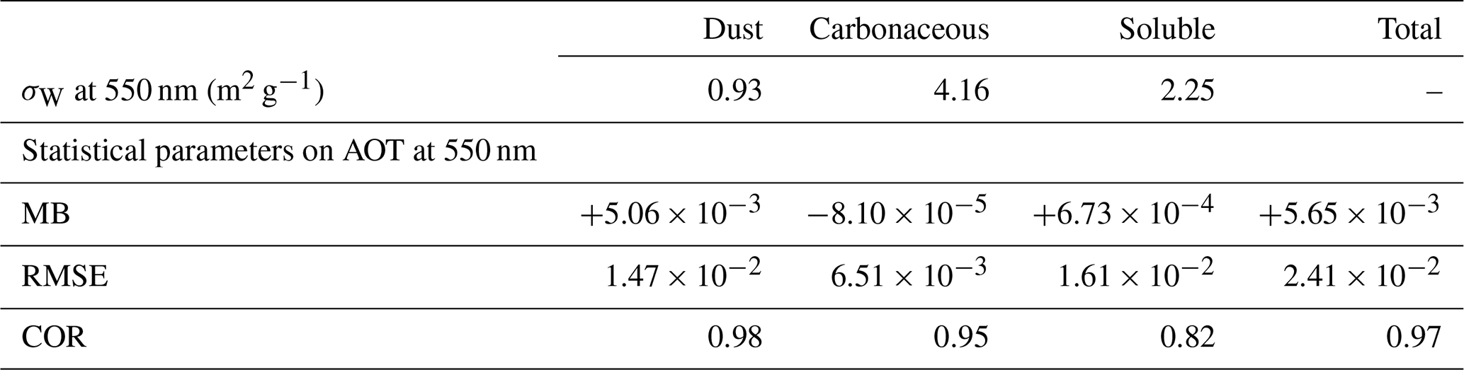
The matching between the AOTs provided by CAMS and those recalculated from the AEC profiles in Eq. (13) is evaluated using statistical parameters defined in Appendix A. Their values are also given in Table 2 for each aerosol type. There is very good agreement, as shown by the mean bias (MB) and root mean square error (RMSE). The correlation coefficient (COR) between CAMS AOTs and AOTs recalculated from mixing ratios is very significant with a value of 0.97. There is an excellent match for dust (not very hydrophilic) and carbonaceous aerosols. The correlation is slightly weaker for soluble aerosols but still shows a COR of 0.82 with a very small bias.

3.2.2 Optical properties at the lidar wavelength of 355 nm

CAMS products contain AOTs for the different classes of aerosol compounds. These AOTs are provided at different wavelengths. The wavelengths closest to the lidar wavelength are used, i.e. 469 and 550 nm. This allows the Ångström exponent (A) predicted by the model to be derived. It is then used to convert the AOT at 550 nm (τ_a550) to the AOT at 355 nm (τ_a355) using the relationship (Ångström, 1964):

$$\begin{array}{}\text{(14)}& {\mathit{\tau }}_{\mathrm{a}\mathrm{355}}={\mathit{\tau }}_{\mathrm{a}\mathrm{550}}\cdot {\left({\displaystyle \frac{\mathrm{355}}{\mathrm{550}}}\right)}^{-A}\end{array}$$

A similar relationship to that in Eq. (10) exists for the AEC. However, as the Ångström exponent is calculated based on the total AOT, it may vary between different aerosol species. It is not possible to fully separate the contributions using the available EAC4 data. Therefore, the Ångström exponent for dust-like particles has been assumed to be the smallest value found in photometric measurements (see Fig. 3) and in the CAMS data, i.e. A_D ≈ 0.3. It is therefore possible to calculate the Ångström exponent (A_CS) for the carbonaceous and soluble components in a coupled system using the following equation:

$$\begin{array}{}\text{(15)}& A_{\mathrm{CS}}=-{\displaystyle \frac{\log \left(\frac{{\mathit{\tau }}_{\mathrm{a}\mathrm{355}}-{\left(\frac{\mathrm{355}}{\mathrm{550}}\right)}^{-A_{\mathrm{D}}}\cdot {\mathit{\tau }}_{\mathrm{a}\mathrm{550}}^{\mathrm{Dust}}}{{\mathit{\tau }}_{\mathrm{a}\mathrm{550}}^{\mathrm{Carbonaceaous}}+{\mathit{\tau }}_{\mathrm{a}\mathrm{550}}^{\mathrm{Soluble}}}\right)}{\log \left(\frac{\mathrm{355}}{\mathrm{550}}\right)}}\end{array}$$

In practice, taking this relationship or the Ångström exponent for the total AOT has a weak effect on the statistical results presented below.

4 Vertical profiles of aerosol layers

This section presents the results of the inversion of lidar profiles. As previously mentioned, the inversion is only performed during the nights between 23:00 and 05:00 LT.

4.1 Night-to-night evolution of lidar-derived aerosol optical properties

Figure 5 presents the temporal evolution of the vertical profiles of AEC (Fig. 5a), PDR (Fig. 5b) and LR (Fig. 5c). Throughout the observation period, the lower troposphere (below 1–1.5 km a.m.s.l.) has been found to be the most aerosol–laden. AECs greater than 0.15 km⁻¹ are frequently observed. However, these are not necessarily associated with high PDRs, despite the arid conditions around San Pedro Alcantara. On many profiles, layers with a PDR greater than 10 % appear quickly as altitude increases up to ∼ 7 km a.m.s.l. They are indicative of the presence of dust-like particles, which are often found in such environments. As for PDR, LR varies greatly over time and along profiles. A wide range of LR values has been observed for dust or pollution aerosols (Mallet et al., 2022), particularly in the Mediterranean region. This diversity is obviously linked to the origin of the particles and their atmospheric ageing, as well as with air mass mixing. Note that when AEC is low (≲ 0.02 km⁻¹), LR and PDR cannot be determined with sufficient accuracy and are not plotted.

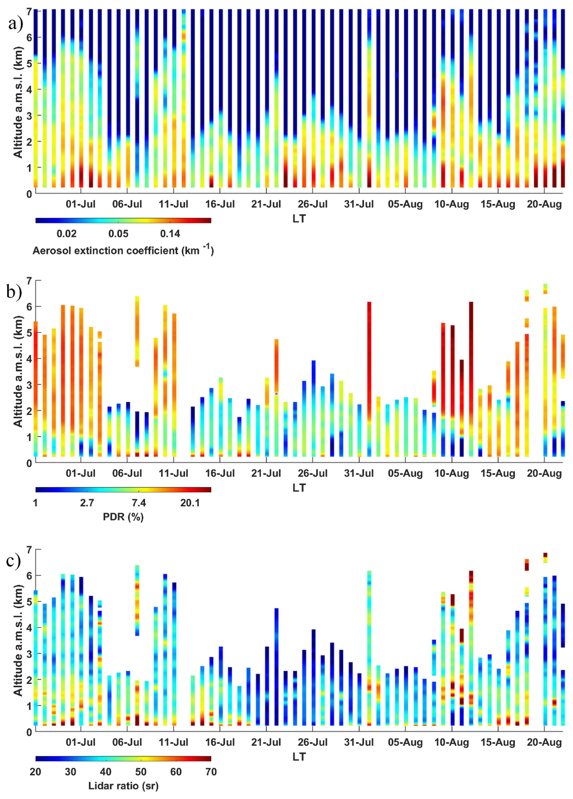
Figure 5 Temporal evolution of the mean night-time profiles derived from the N₂–Raman lidar is shown for (a) the aerosol extinction coefficient, (b) the linear particle depolarisation ratio (PDR), and (c) the lidar ratio. The mean values are displayed for the period between 23:00 and 05:00 LT on a nightly basis.

4.2 Highlight of aerosol classification by Raman lidar

In order to identify changes in aerosols more accurately over time and within the air column, it is best to rely on simultaneous LR and PDR measurements. The LR and PDR pair has been demonstrated to be the most discriminating technique for separating dusts, soluble and polluted aerosols (Groß et al., 2013, 2015; Chazette et al., 2016a).

4.2.1 Parameterisation and assumptions

Dust aerosols over the western Mediterranean Sea are attributable to the long-range transport of Saharan dust. These aerosols are typically associated with LRs between 30 and 80 sr (Papayannis et al., 2008), specifically for high PDRs, above 10 % and up to ∼ 30 %. This variability is explained by the level of mixing with other aerosol types and the nature of soils in uplift areas. In the overview by Mallet et al. (2022), the reported LR values at 355 nm are predominantly between 32 and 84 sr, including polluted dust aerosols. In Groß et al. (2015), however, they are closer to 55 ± 20 sr, and for the same authors, the PDRs are of the order of 25 ± 15 %. These values include those provided by Chazette and Totems (2023), which range from 45 to 70 sr for the LR and from 20 ±  15 % for the PDR.

Marine aerosols have been found to have low LRs, ranging from 20 to 30 sr (Flamant et al., 1998), which corresponds to a very low PDR. However, these particles are often mixed with polluted aerosols or dust, which increases their LR and PDR. Mallet et al. (2022) reported LR of ∼ 25 ± 6 sr, which is very close to the values given in Groß et al. (2015) (∼ 25 ± 10 sr). The PDR remains low due to the spherical characteristics of these highly hydrophilic aerosols, with values of ∼ 3 ± 3 % (e.g. Chazette et al., 2019; Groß et al., 2015).

The LR of pollution and biomass fire aerosols is highly variable depending on the combustion source, with values of ∼ 60 ± 20 sr (Chazette et al., 2019; Groß et al., 2015). Mallet et al. (2022) also report smoke-like aerosols with an LR between 42 and 73 sr. It should be noted that the combustion temperature influences the LR by affecting the chemical composition of the aerosols. It also influences the PDR, mainly in the event of strong thermal convection, whereby terrigenous particles can be lifted from the surface, leading to PDRs of the order of 8 % (Chazette et al., 2016a). By contrast, the PDRs typically range from 2 % to 3 % for young aerosols, rising to over 6 % after long-range transport and potential mixing with other air masses. Groß et al. (2015) reported PDRs of ∼ 3 ± 3 % for smoke-like aerosols. These values are similar to those provided by Chazette and Totems (2023).

All of these values are obtained from short-term campaigns in very specific locations and are few in numbers. Significant variation can clearly occur depending on the degree of particle mixing and potential ageing during transport. Figure 2 in Floutsi et al. (2023) clearly shows the overlap between the different aerosol classes in the LR and PDR ranges at 355 nm, as well as the potential for distinguishing them from one another.

Figure 5 also allows us to determine the range of variation for the LR and PDR. For dust-like aerosols, LR varies from approximately 30 to 70 sr, whereas PDR is around 20 ± 10 %. This is broadly consistent with previous reports. Similarly, the LR for marine-like (soluble) aerosols tends to be between 20 and 40 sr, with PDRs ranging from ∼ 0 % to 8 %. Pollution-like (carbonaceous) aerosols, on the other hand, are associated with LR values between 40 and 80 sr and PDRs of up to 10 %.

Taking the above into account, the following colour combination is proposed to help identify the three distinct aerosol types and their potential for mixing by using two-dimensional normal distributions (C). The first dimension is defined on the PDR and the second on the LR. For each primary colour (red, green, and blue):

$$\begin{array}{}\text{(16)}& C={\displaystyle \frac{\mathrm{1}}{\mathrm{2}\cdot \mathit{\pi }\cdot {\mathit{\sigma }}_{{\mathit{\delta }}_a}\cdot {\mathit{\sigma }}_{L_r}}}\cdot e^{-\frac{\mathrm{1}}{\mathrm{2}}\cdot \left[\frac{{\left({\mathit{\delta }}_a-{\mathit{\delta }}_{ao}\right)}^{\mathrm{2}}}{{\mathit{\sigma }}_{{\mathit{\delta }}_a}^{\mathrm{2}}}+\frac{{\left(L_r-L_{ro}\right)}^{\mathrm{2}}}{{\mathit{\sigma }}_{L_r}^{\mathrm{2}}}\right]}\end{array}$$

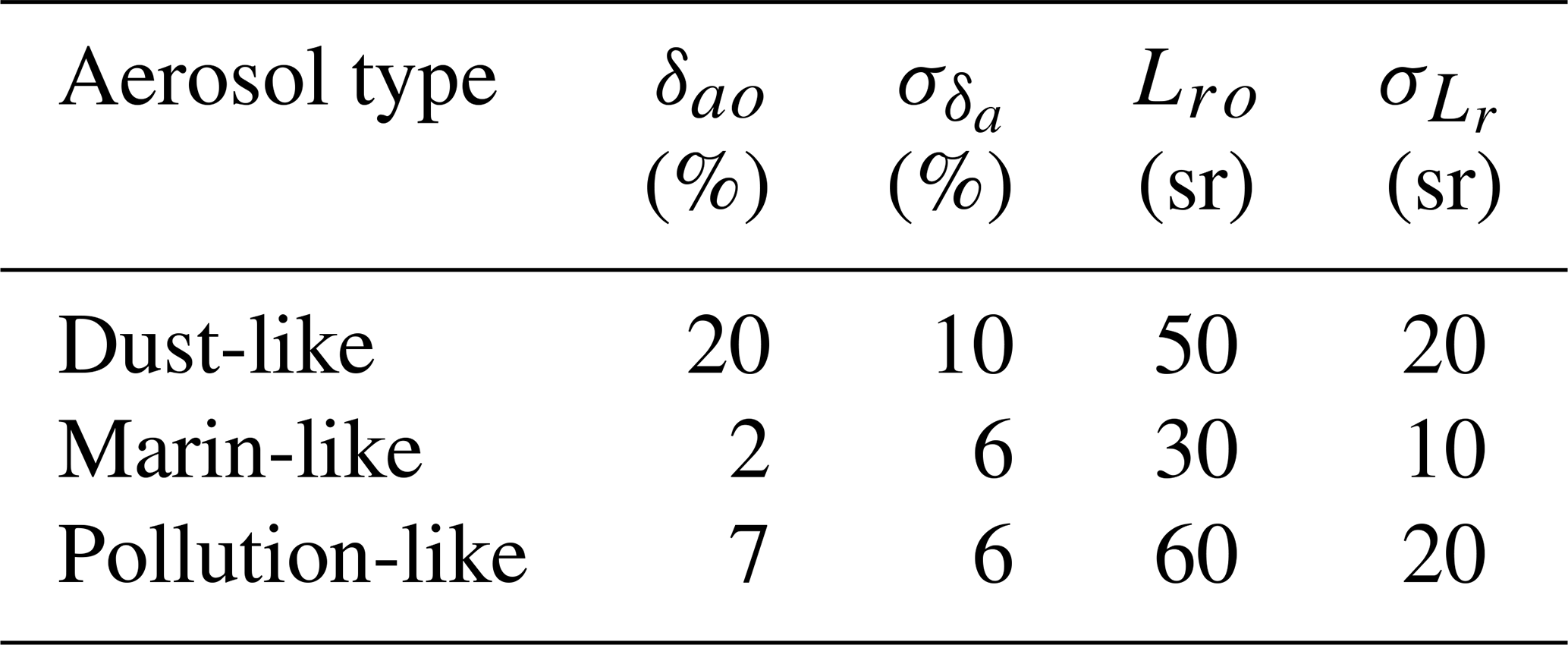
The mean values (δ_ao and L_ro) and standard deviations (${\mathit{\sigma }}_{{\mathit{\delta }}_a}$ and ${\mathit{\sigma }}_{L_r}$) for the PDR and LR, respectively, are given in Table 3. These values consider the possible ranges of PDR and LR for each aerosol type as presented previously. The exponential form clarifies potential mixtures by assigning lower weights to extreme values, while still taking the large variability associated with each type of aerosol into account.

Table 3 Mean linear particle depolarization ratio (δ_ao) and lidar ratio (L_ro) for each aerosol type, along with their respective standard deviations (${\mathit{\sigma }}_{{\mathit{\delta }}_a}$ and ${\mathit{\sigma }}_{L_r}$).

Unlike the approaches proposed by Wandinger et al. (2023) and Floutsi et al. (2024), which require initial conditions and prior estimates of the variance–covariance matrices of both the observables and the lidar simulator, the method used here does not rely on an optimal estimation approach. It is therefore simpler to implement. Furthermore, it is based on ground-based measurements, for which the signal-to-noise ratio is significantly higher than that of spaceborne measurements such as those performed by ATLID. In the latter case, the implementation of an optimal estimation approach may be more appropriate, as it enables smoothing of the retrieved information.

4.2.2 Classification results

Figure 6 shows the temporal evolution of the three aerosol classes and highlights their potential mixing, revealing a strong presence of dust particles (red trend) at the beginning and end of the field campaign. All the main dust contributions are due to Saharan air mass transport, which is well highlighted on MODIS aerosol products (e.g. see https://worldview.earthdata.nasa.gov/, last access: 27 April 2026). These particles mix with the other types of aerosols in the lower layers below 1.5 km above sea level, where pollution events (green trend) can be observed alongside the marine contributions (blue trend). These mixtures are not dependent on local occurrence; instead, they are primarily linked to the long-range transport of diverse aerosol plumes by convergent dynamic processes.

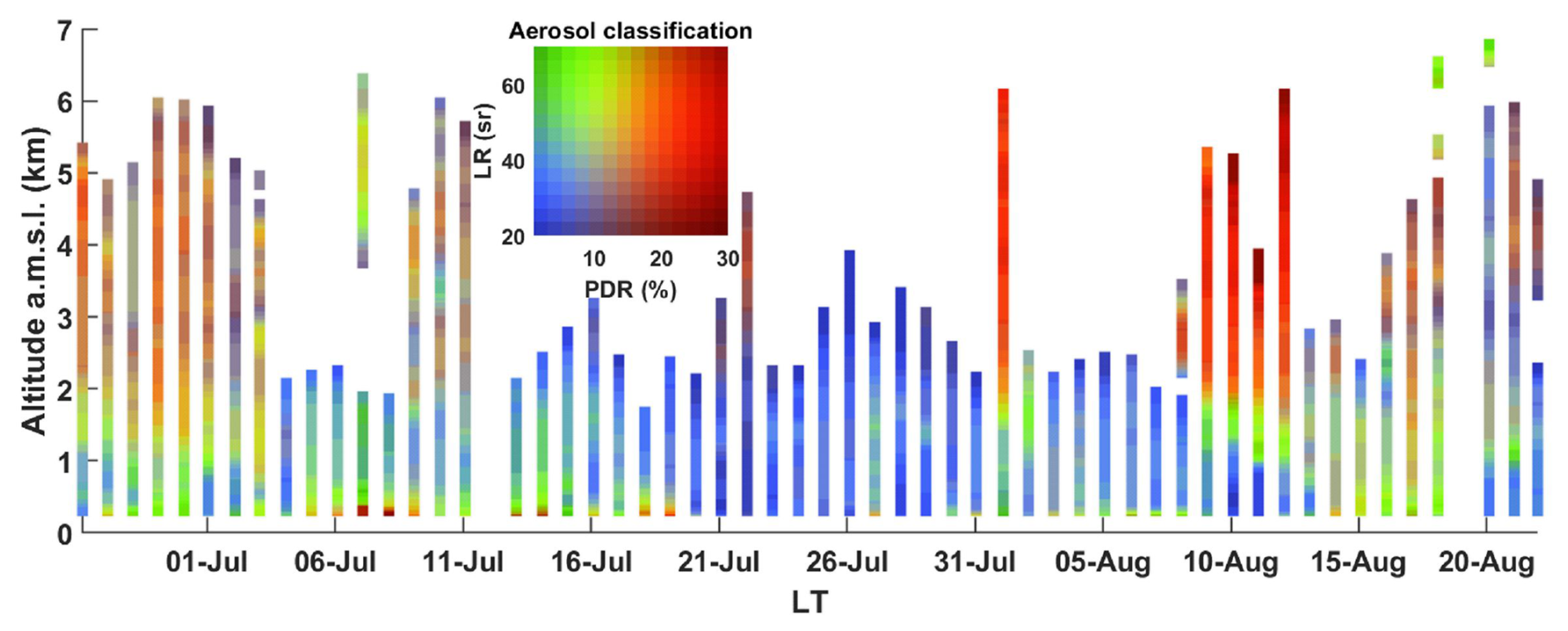
Figure 6 Temporal evolution of the aerosol classification performed using the linear particle depolarisation ratio (PDR) and the lidar ratio (LR). Aerosols of marine origin tend towards blue, pollution aerosols towards green, and terrigenous aerosols towards red.

4.2.3 Sensitivity study

A sensitivity analysis using a Monte Carlo approach was performed to assess the reliability of this optical apportionment based on lidar measurements, as described by Royer et al. (2011a). Uncertainties in LR and PDR were assumed to be up to 5 % (relative) for LR and 2 % (absolute) for PDR. Figure 7 presents the results for the three particle types. As can be seen, the influence of the uncertainties on lidar-derived optical parameters is small, remaining below 5 % for each aerosol type. This demonstrates the robustness of the classification with respect to realistic uncertainties associated with lidar measurements.

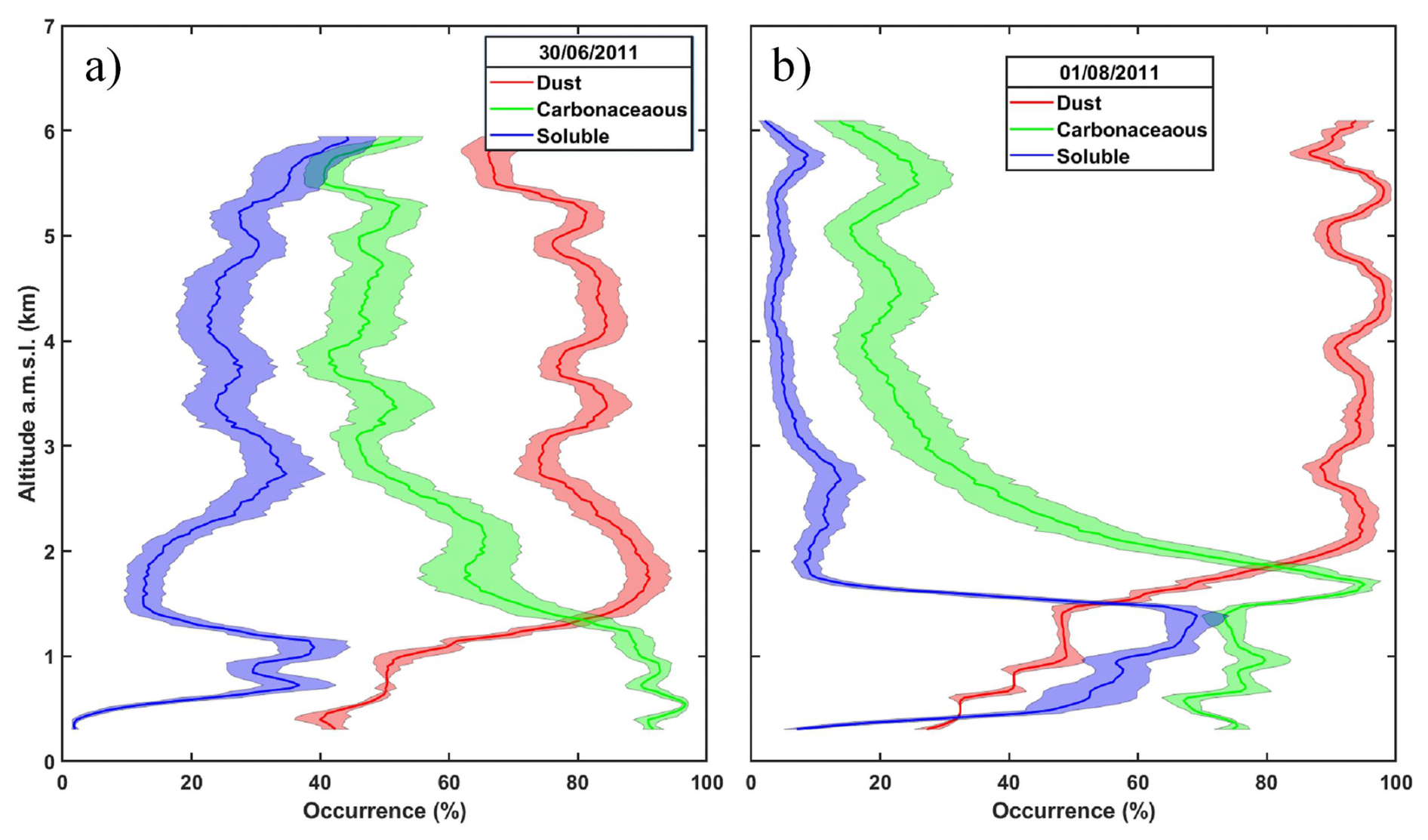
Figure 7 Uncertainty on the occurrences of each aerosol type due to statistical error on both the lidar ratio (LR, 5 % in relative) and linear particle depolarization ratio (PDR, 2 % in absolute) on 30 June and 1 August 2011. The mean value is given by the continuous lines and the standard deviation by the shaded area.

4.3 Comparison with sun photometer measurements

During the day, sun photometer measurements provide information on the nature of the aerosols present in the air. Angstrom exponents of less than 0.5, which are associated with higher optical thicknesses (Fig. 3) are generally indicative of dust events. Saharan dust events with AOT > 0.6 are clearly highlighted by photometric measurements during the following periods in 2011: 26 June–4 July, 8–12 July, 20–22 July, 8–12 August and sporadically from 16 to 22 August. Their origin is mainly located between Morocco and Algeria, towards the great western erg (Chazette, 2020). In June, their origin is more distant, with a plausible source located in northern Mauritania as highlighted from airborne measurements (Ryder et al., 2015). The plume has recirculated over the Atlantic before entering the Mediterranean via Gibraltar. Note that on 25 July, the AOT reached 0.7 for A ∼ 1.4 during the day, which was not detected by the lidar during the night. This is indicative of the sporadic presence of pollution or biomass burning aerosols.

5 Consistency with CAMS simulations

Lidar measurements do not allow for quantitative separation of the optical contributions of individual aerosol compounds. Consistency between lidar measurements and CAMS data can therefore only be achieved for the total aerosol contribution to the optical parameters. The total AOTs are provided directly by the CAMS database whereas, as explained in Sect. 3.2, the vertical extinction profiles must be derived using the available mixing ratios in the database. The nature of the aerosols is identified by combining the LR and PDR. As previously seen, these vary across different ranges depending on the type of particle.

5.1 Aerosol optical thickness

Figure 8 shows the temporal evolution of AOTs derived from CAMS reanalyses for each type of bulk aerosol composition at the ground-based site. The five Saharan dust events previously identified are clearly visible.

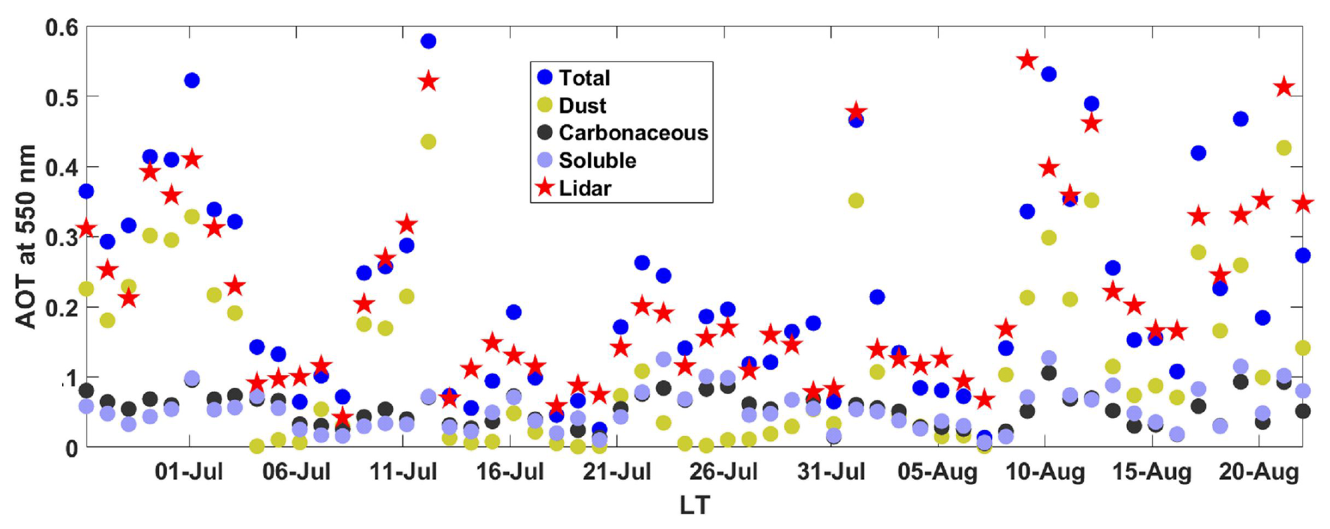
Figure 8 Superimposition of the temporal evolution of the aerosol optical thickness (AOT) derived from CAMS (total aerosol contribution and, dust, carbonaceous and soluble compounds) and from the N₂–Raman lidar at 550 nm using the sun photometer-derived Ångström exponent.

There are two approaches to comparing AOTs. The first consists of doing so at a wavelength of 550 nm by converting the lidar-derived AOTs to the same wavelength. To do this, an interpolation of the Ångström exponents retrieved from the sun photometer is used (red curve in Fig. 3). The AOTs derived from the lidar measurements and the sun photometer are also shown in Fig. 8. The second method consists of bringing the AOTs derived from the model to the lidar wavelength using the Ångström exponent predicted by CAMS. The statistical results of these two approaches are shown at the top of Table 4.

Table 4 Statistical parameters of the comparison between the aerosol optical thicknesses derived from the Raman lidar and the corresponding CAMS products (lidar-CAMS): mean bias (MB), root mean square error (RMSE) and correlation coefficient (COR).

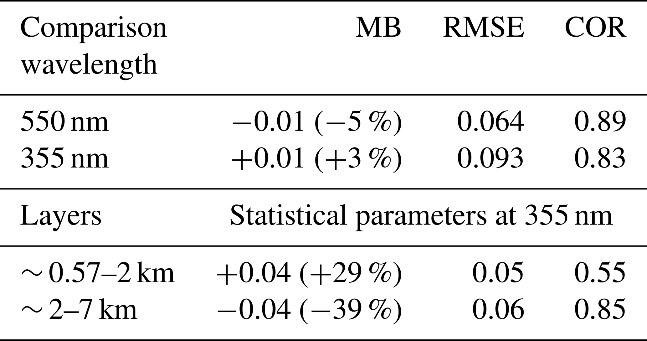
For both approaches, there is a very small underestimation of the total AOT by CAMS (−0.01) compared to lidar. The CORs are very similar, with values exceeding 0.83. This tends to show that CAMS satisfactorily reproduces the variability of integrated aerosol content throughout the lidar measurement period. The RMSEs are greater at 355 nm (∼ 0.09) than at 550 nm (∼ 0.06). This difference can be explained by the inclusion of an Ångström exponent from the modelling. This exponent introduces additional uncertainties possibly related to poor prediction of the size distribution and/or chemical composition of aerosols. When comparisons are made at 550 nm, the uncertainties are lower because the interpolation of sun photometer measurements taken at night is more likely to reflect reality. Hence, working at the lidar wavelength of 355 nm better highlights the differences between the lidar observation and the CAMS products.

It is important to note that achieving a satisfactory score for total optical thickness does not necessarily guarantee the same level of quality for profiles.

5.2 Vertical profile of the aerosol extinction coefficient

The same statistical study was carried out on the AEC for the different altitude levels of CAMS products at the wavelength of 355 nm. This wavelength is more suitable for assessing modelling reliability. Due to the significant difference in resolution between the CAMS and lidar profiles, spline interpolation was applied (Perperoglou et al., 2019). The results presented here are at the model resolution. Similar results are obtained when the vertical resolution of the lidar is used and spline interpolation is applied to the model data. It is worth noting that model's resolution is higher for the lower layers, meaning they are estimated more accurately. However, for the upper layers, the thickness of the desert dust clouds limits the effect of the small model's vertical resolution.

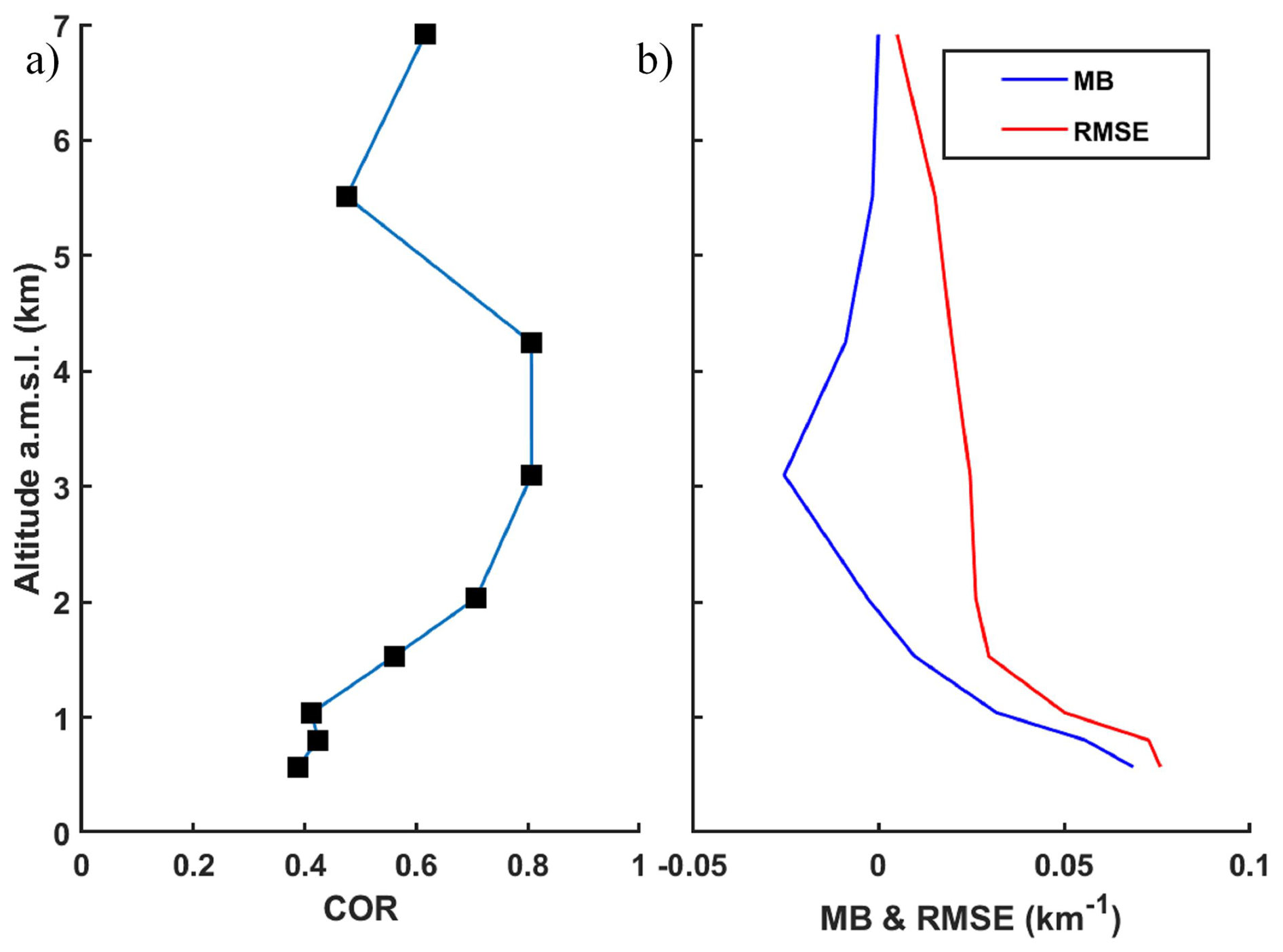
Figure 9 Statistical parameters calculated on the first nine altitude levels of CAMS when comparing lidar measurements with CAMS products at 355 nm. The vertical profiles show: (a) the correlation coefficient (COR) and (b) the mean bias (MB, lidar – CAMS) and the root mean square error (RMSE) on the aerosol extinction coefficient.

The results are shown in Fig. 9. The MB varies significantly with altitude: it is positive near the surface and can be negative aloft, where desert aerosol layers are predominantly located. The RMSE is significantly higher near the surface. This is associated with fairly low CORs (∼ 0.4), indicating that CAMS products struggle to accurately represent the conditions in the planetary boundary layer (PBL). In the upper layers, the COR reaches values slightly above 0.8, indicating that the model accurately reproduces the temporal variability of desert aerosol plumes. Table 4 summarises these results in terms of AOT in two layers: the lower layer (below 2 km a.m.s.l.) and the upper layer (between 2 and 7 km a.m.s.l.), which mainly contains desert aerosols. As shown on the vertical profiles, the most notable difference is in the COR, which averages 0.55 in the lower layer and 0.85 in the upper layer. There is also a significant positive bias in the lower layer (+0.04 % or +29 %), indicating an underestimation by CAMS products. This may be linked to errors in aerosol emissions that can be directly attributed to the emission inventory, and/or the more complex dynamics of the lower layer in coastal regions. For the upper layer, the bias is negative (−0.04 % or −39 %), indicating a tendency for the model to overestimate dust concentrations. This may be caused by factors similar to those mentioned above, as well as discrepancies in the horizontal position and vertical spread of the dust plume. Furthermore, the altitude of aerosol layers can vary considerably over time, particularly between periods with and without long-distance transport events. This aspect is more difficult to quantify statistically in this field campaign because, although it lasted approximately 2 months, it did not capture enough transitions between transport regimes.

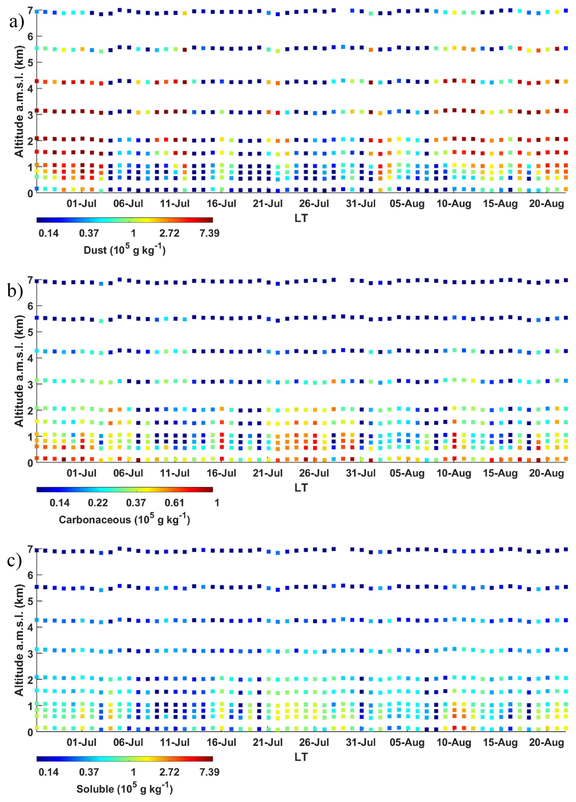
Figure 10 Temporal evolution of the profiles of mass mixing ratios derived from CAMS nearest night-time is shown for the following aerosol compounds: (a) the soluble (sea salt and sulphate), (b) dust, and (c) carbonaceous (black and organic carbon). The vertical resolution is that of the CAMS products.

5.3 Aerosol identification

Figure 10 shows the temporal evolution of the mass mixing ratios of the three bulk aerosol compositions, as derived from the CAMS reanalysis. Qualitatively, the altitude and time locations of the dust plume (Fig. 10a) correspond to the optical apportionment of the aerosols derived from LAASURS (Fig. 6). This demonstrates that CAMS reanalyses provide an excellent representation of mesoscale aerosol transport, uplift and dispersion processes. Polluted aerosols (Fig. 10b) are also well represented in terms of their temporal and vertical extent. Between 21 and 31 July, a slightly more marine trend emerges (Fig. 10c), which could be classified as “dusty marine”. During this period under 1.5 km a.m.s.l., the composition of the aerosols appears to be a variable mixture of dust, carbonaceous and soluble compounds. This results in a range of intermediate values for both the LR and the PDR. In the Mediterranean region, the likelihood of desert aerosols combining with other atmospheric particles explains the variability of the LR observed in different locations within the basin (Mallet et al., 2022; Papayannis et al., 2008).

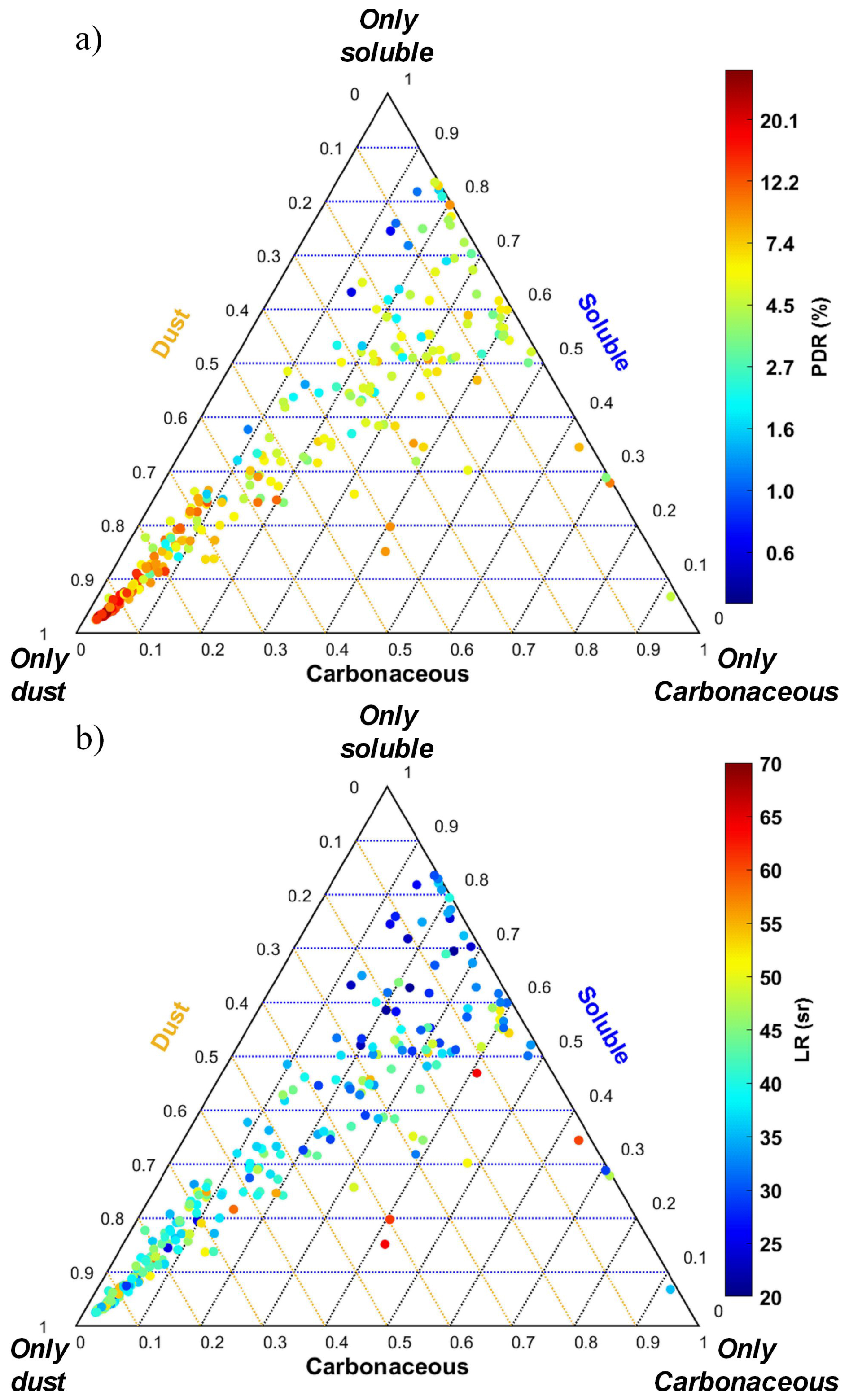
Figure 11 Ternary diagram established from the aerosol compounds derived from CAMS: dust, carbonaceous and soluble compounds. Each colour dot corresponds to lidar-derived optical properties: (a) particulate depolarization ratio (PDR) and (b) lidar ratio (LR). The projections onto the sides of the equilateral triangle are colour coded as follows: orange for dust aerosols, blue for soluble aerosols, and black for carbonaceous aerosols.

The correspondence between lidar and CAMS for identifying aerosol types is clearly shown in the ternary diagrams in Fig. 11. For each time period and CAMS level, the LR (Fig. 11a) and PDR (Fig. 11b) are displayed using a colour scale. On these diagrams, pure compounds are located at the vertices of the equilateral triangle. Most high PDR values correspond to points close to the “dust” vertex of the triangle (CAMS estimates over 60 % “dust”), and are mainly associated with intermediate LR values (approximately 45 sr), as is often found in the literature (e.g. Papayannis et al., 2005). The contribution of carbonaceous compounds to the composition of aerosols is significantly lower than that of soluble compounds. Nevertheless, these diagrams clearly show that the three components are often mixed. It should be noted that there were no significant biomass fires in Andalusia during the summer of 2011.

6 Conclusion

Considerable progress has been made in modelling aerosol transport since the FENNEC campaign in 2011. This has been accomplished through more accurate inventories of aerosol sources and improving the spatial resolution of the models, particularly in the vertical dimension. However, additional experimental validation methods are needed to increase confidence in modelling. This should primarily involve using resolved measurements taken directly in the atmospheric column, such as those provided by lidar. Consequently, the data acquired from the ground-based site in San Pedro Alcantara from June to August 2011 provide a unique opportunity to compare the CAMS reanalyses with the optical products of the LAASURS N₂–Raman lidar at 355 nm. During the FENNEC programme, LAASURS monitored aerosols with high vertical resolution (100 m). This monitoring aimed to accurately locate the transport of Saharan aerosols in southern Spain, assess their frequency and intensity, and analyse how they mix with other, more local, aerosol layers. The PDR and LR pairs were derived from night-time measurements to ensure the lidar range sampled the desert aerosol layers above 7 km a.m.s.l. This makes it possible to identify the aerosols and their mixtures in the vertical profiles.

In the free troposphere, the CAMS reanalyses (EAC4) were found to be in agreement with the geophysical products derived from optical lidar measurements for dust layers. This is particularly notable for the AOTs. The reanalyses accurately reproduce dust events in terms of both time and vertical extends with COR ∼ 0.85. However, there is an overestimation of the AOT at 355 nm (∼ 39 %) compared to the Raman lidar products.

In the lower troposphere, below 2 km a.m.s.l., the mixing of pollution (characterised by the carbonaceous component) with marine (characterised by the soluble component) and dust contributions is also accurately reproduced throughout the 2-month experiment. Nevertheless, the correlation between lidar measurements and CAMS reanalyses is significantly lower (0.55). It is associated with an underestimation of the AOT contribution of this layer of around +0.04 (+29 %) at 355 nm, which may be due to an incorrect representation of emission processes. However, it should be noted that the neglect of aerosol hygroscopicity may also affect this result. Such an omission may be present in the model itself, given that a number of assumptions have been made. Alternatively, it may arise from the calculation of aerosol extinction coefficients performed in this study. Note that, conversely, lidar measurements account for the hydrophilic nature of aerosols.

In the entire atmospheric column, good agreement is observed in the temporal evolution of total AOT derived from CAMS and lidar. This is associated with a small mean bias (+0.01 % or 3 %) and a significant correlation coefficient (0.83). This is primarily due to the fact that dust aerosols dominated the aerosol load during the FENNEC field campaign, and the reanalyses better represent them in terms of total AOT. There is a compensation effect between the upper and lower layers: the reanalyses do not distribute dust particles perfectly across these two layers, with an overestimation in the upper layer and an underestimation in the lower layer.

These results show that assimilating lidar measurements can impose significant constraints on aerosol transport models (Wang et al., 2013, 2014b). This is an important area on which to focus on, given the current risks for the climate and air quality. Note that the optical aerosol classification technique used here for a single-wavelength Raman lidar at 355 nm can also be used with a high spectral resolution lidar, such as the Atmospheric Lidar (ATLID) of the Earth Clouds, Aerosols and Radiation Explorer mission (EarthCARE, https://earth.esa.int/eogateway/missions/earthcare, last access: 28 April 2026).

Appendix A: Statistical parameters

The statistical indicators used to evaluate the consistency between lidar-derived (α_a,lidar) and CAMS-derived (α_a,cams) AEC are the mean bias (MB), the root mean square error (RMSE) and the (Pearson) correlation (COR). These metrics are commonly used to assess model performance (Boylan and Russell, 2006; Tombette et al., 2008). For a given time t and altitude z, the MB is given by the following relationship:

$$\begin{array}{}\text{(A1)}& \text{MB}\left(z\right)=\langle {\mathit{\alpha }}_{\mathrm{a},\mathrm{lidar}}(t,z)\rangle -\langle {\mathit{\alpha }}_{\mathrm{a},\mathrm{cams}}(t,z)\rangle \end{array}$$

The RMSE is given by:

$$\begin{array}{}\text{(A2)}& \text{RMSE}\left(z\right)=\sqrt{{\text{RMSD}}^{\mathrm{2}}-{\text{MB}}^{\mathrm{2}}}\end{array}$$

with the root mean square difference (RMSD) given by:

$$\begin{array}{}\text{(A3)}& \text{RMSD}\left(z\right)=\sqrt{\langle {\left({\mathit{\alpha }}_{\mathrm{a},\mathrm{lidar}}(t,z)\rangle -\langle {\mathit{\alpha }}_{\mathrm{a},\mathrm{cams}}(t,z)\right)}^{\mathrm{2}}\rangle }\end{array}$$

The COR is expressed as follows:

$$\begin{array}{}\text{(A4)}& \text{COR}\left(z\right)={\displaystyle \frac{<\begin{array}{c}\left({\mathit{\alpha }}_{\mathrm{a},\mathrm{lidar}}(t,z)-\langle {\mathit{\alpha }}_{\mathrm{a},\mathrm{lidar}}(t,z)\rangle \right)\\ \cdot \left({\mathit{\alpha }}_{\mathrm{a},\mathrm{cams}}(t,z)-\langle {\mathit{\alpha }}_{\mathrm{a},\mathrm{cams}}(t,z)\rangle \right)\end{array}>}{\sqrt{\begin{array}{c}\langle {\left({\mathit{\alpha }}_{\mathrm{a},\mathrm{lidar}}(t,z)-\langle {\mathit{\alpha }}_{\mathrm{a},\mathrm{lidar}}(t,z)\rangle \right)}^{\mathrm{2}}\rangle \\ \cdot \langle {\left({\mathit{\alpha }}_{\mathrm{a},\mathrm{cams}}(t,z)-\langle {\mathit{\alpha }}_{\mathrm{a},\mathrm{cams}}(t,z)\rangle \right)}^{\mathrm{2}}\rangle \end{array}}}}\end{array}$$

The AOTs can also be treated with the same equations by replacing the AEC with the respective AOTs.