Extended TCKF1D-Var framework for Mie–Raman lidar boundary layer water vapor profiling: insights into nocturnal preprecipitation moisture evolution

Accurate characterization of boundary-layer water vapor prior to nocturnal heavy precipitation remains challenging due to limited observational capability. In this study, we build upon a previously developed and validated thermodynamic- and cloud-microphysics-constrained Kalman filter one-dimensional variational (TCKF1D-Var) framework by extending it to incorporate nitrogen and water vapor Raman channel observations from the China Meteorological Administration Mie–Raman lidar (MRL) network. A physics-informed lidar observation operator based on the classical Raman lidar formulation is developed, together with a data-driven calibration component to account for time-varying instrumental and aerosol-related uncertainties. In addition, process and observation error covariance matrices are dynamically estimated within the Kalman filter framework to enhance retrieval robustness. The method is evaluated against co-located radiosonde observations launched prior to nocturnal heavy precipitation events (224 cases in total) at 56 MRL–radiosonde co-located stations across China in 2025. The retrieved water vapor mass mixing ratio profiles, with a vertical resolution of 30 m and a temporal resolution of 30 min, exhibit consistently reduced mean bias and root mean square error compared to ERA5 profiles as priori, with the largest improvements found in the 1.2–3.0 km layer. Analysis of nocturnal heavy precipitation cases further demonstrates that the retrievals capture coherent pre-precipitation moisture evolution. These results highlight the potential of combining physically constrained retrieval frameworks with Raman lidar observations for improved monitoring of boundary-layer moisture.

1 Introduction

Nocturnal precipitation over China is frequently characterized by abrupt initiation, intense short-duration rainfall, and high societal impact (Luo et al., 2016, 2020; Chen et al., 2021; Zhang et al., 2025a; Gao et al., 2026). Previous studies have shown that rapid variations in boundary-layer moisture play a critical role in both the triggering and rapid intensification of nighttime precipitation (Li et al., 2026; Richardson et al., 2024; Sun et al., 2025). In particular, localized moisture accumulation and vertical redistribution within the boundary layer can precondition the atmosphere for deep convection (Ahmed et al., 2020; Kirshbaum et al., 2018; Behrendt et al., 2011; Wulfmeyer et al., 2011), even in the absence of strong large-scale forcing (Kirshbaum, 2011; Lu et al., 2025). These features highlight the necessity of monitoring high-resolution temporal and vertical variations of boundary-layer water vapor during nighttime. However, capturing such rapid and fine-scale moisture evolution remains challenging for existing observing systems: conventional radiosonde observations provide high-accuracy thermodynamic profiles but are typically limited by sparse temporal sampling; satellite-based infrared and microwave sounders offer broad spatial coverage, however, their vertical resolution and sensitivity within the planetary boundary layer are often insufficient, particularly under cloudy and precipitating conditions; ground-based microwave radiometers can provide continuous thermodynamic observations but generally suffer from relatively coarse vertical resolution and reduced retrieval accuracy near sharp moisture gradients (Richter et al., 2026; Mayer et al., 2012; Oue et al., 2022; Wulfmeyer et al., 2008, 2015).

Ground-based active remote sensing provides a promising pathway to address the limitations listed above. Notably, Raman lidars operating at a laser wavelength of 354.7 nm can simultaneously detect nitrogen Raman signals at 386.7 nm and water vapor Raman signals at 407.5 nm, enabling the profiling capability of atmospheric water vapor (Vaughan et al., 1988; Di Girolamo et al., 2017; Lange et al., 2019, 2025; Whiteman et al., 2006, 2010; Wulfmeyer et al., 2010; Behrendt et al., 2002). Compared with passive instruments such as ground-based microwave radiometers and hyperspectral infrared sounders, Raman lidars offer substantially higher vertical resolution and are capable of resolving detailed moisture structures within the boundary layer (Wulfmeyer et al., 2015; Gambacorta et al., 2025). In addition, Raman lidar offers more direct water vapor measurements with less dependence on a priori requirements compared to passive remote sensing techniques (Whiteman et al., 2012; Foth and Pospichal; 2017; Filioglou et al., 2017). These advantages make 354.7 nm Raman lidar systems an ideal observational tool for investigating boundary-layer moisture evolution associated with nocturnal precipitation.

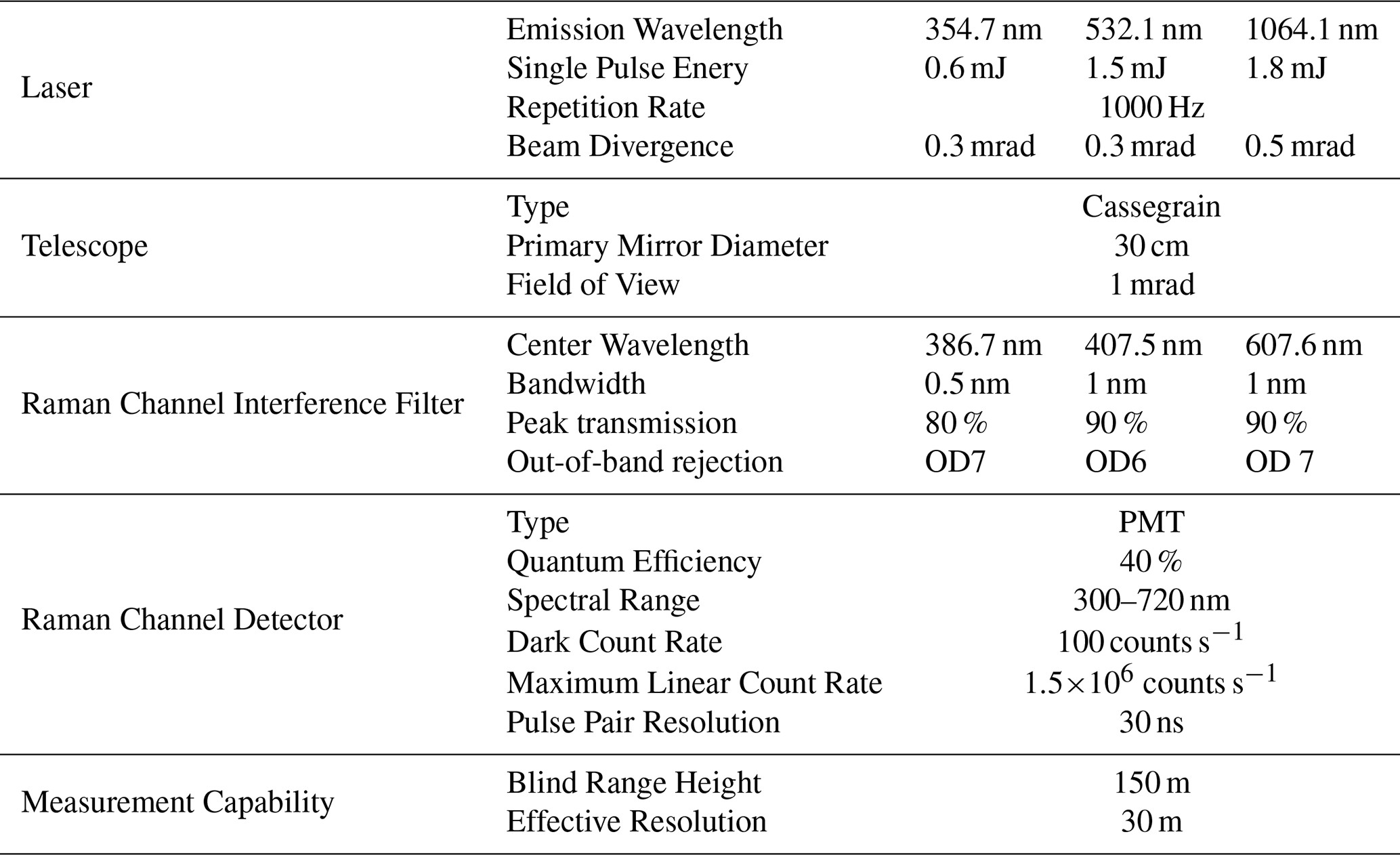
To achieve sufficient signal-to-noise ratio, Raman lidar systems typically require pulse energies exceeding 100 mJ (Wandinger, 2005). However, recent technological advances in micro-pulse laser design have enabled an alternative measurement paradigm based on low single-pulse energy and high repetition rate operation. Specifically, improvements in ultraviolet average power (1–5 W) and reduced beam divergence (0.3–0.5 mrad), combined with the use of large-aperture telescopes (0.3–0.4 m diameter), allow micro-pulse laser-based Raman lidars to compensate for reduced pulse energy through high pulse accumulation, thereby enabling the retrieval of vertical profiles of atmospheric thermodynamic parameters, including water vapor and temperature, under both daytime and nighttime conditions (Di Girolamo et al., 2023). Within this measurement paradigm, the Mie–Raman lidar (MRL) network deployed by the China Meteorological Administration (CMA) operates with a pulse energy of 0.6 mJ at 354.7 nm and repetition rate of 1000 Hz (Shao et al., 2025; Zhang et al., 2025c). Although such systems inherently benefit from high repetition rates, the resulting observations are still subject to significant noise, particularly at short temporal scales, posing challenges for retrieving reliable water vapor mass mixing ratio profiles using conventional inversion approaches. Therefore, there is a clear need for advanced retrieval methods that can fully exploit the nitrogen and water vapor Raman channel observations from these lidars and provide robust estimates of boundary-layer water vapor structure.

In the previous work, we developed a thermodynamic- and cloud-microphysics-constrained Kalman filter one-dimensional variational (TCKF1D-Var) retrieval framework (Zhang et al., 2026b) applied to ground-based microwave radiometer (GMWR) observations to retrieve temperature, humidity, and hydrometeor profiles with high accuracy. This method incorporates moist thermodynamic constraints by using virtual potential temperature as the control variable and improves retrieval stability under cloudy and precipitating conditions by coupling the cloud microphysics scheme with the cost function. The retrieved profiles have demonstrated strong capability in capturing the evolution of boundary-layer thermodynamic conditions prior to the initiation of heavy precipitation.

This study extends the TCKF1D-Var framework to incorporate nitrogen and water vapor Raman channel observations from the MRL network deployed by the CMA. By integrating these measurements within a physically constrained retrieval system, we derive boundary-layer water vapor mass mixing ratio profiles with a vertical resolution of 30 m, same as the native lidar resolution, and a temporal resolution of 30 min. The performance of the proposed method is evaluated using collocated radiosonde observations from 56 stations across China in 2025. Furthermore, we assess the capability of the retrieved profiles to capture pre-precipitation boundary-layer moisture signals by analyzing nocturnal heavy precipitation events observed at the same stations. The remainder of this paper is organized as follows. Section 2 describes the observational instruments, datasets, and the extensions of the TCKF1D-Var framework developed in this study. Section 3 presents the validation of the retrieved water vapor mass mixing ratio profiles and demonstrates their capability to capture boundary-layer moisture variations prior to heavy precipitation. Finally, Sect. 4 provides a summary and concluding remarks.

2 Instrument, Data, and Method

2.1 Mie–Raman lidar

Starting in 2021, CMA initiated the deployment of MRLs and associated instruments at key observational stations (Zhang et al., 2025b; Shao et al., 2025). By the end of 2025, a total of 56 radiosonde stations participating in international data exchange had been co-located with MRLs across China, each providing more than 1 year of operational observations (Fig. 1). The MRL system operates at laser wavelengths of 354.7, 532.1, and 1064.1 nm. The receiver is composed of eight detection channels, among which three are Raman channels centered at 386.7, 407.5, and 607.6 nm, enabling the retrieval of atmospheric water vapor and nitrogen Raman backscatter signals. Detailed system specifications are summarized in Table 1.

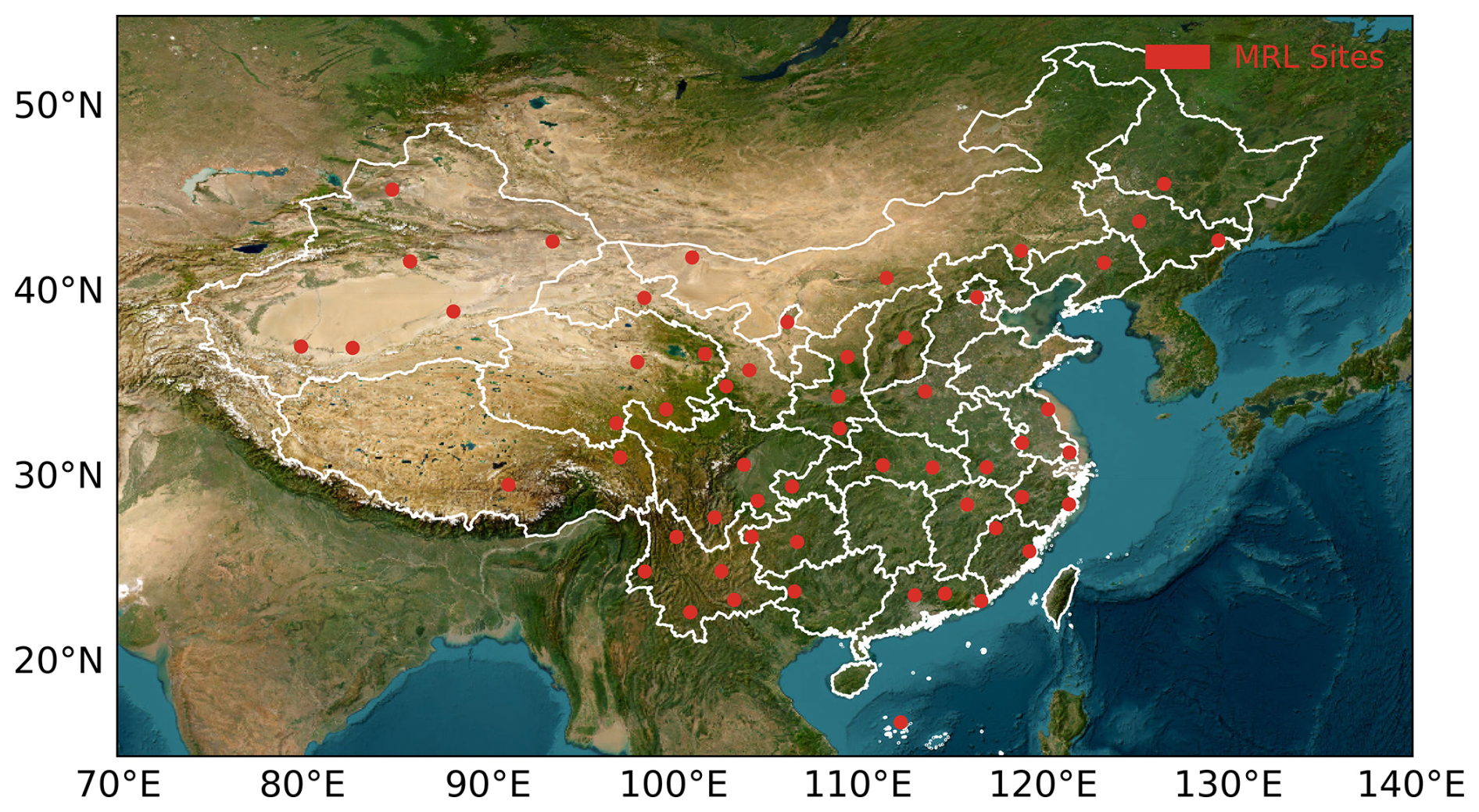
Figure 1 Spatial distribution of the MRL systems co-located with radiosonde stations across China as of the end of 2025. A total of 56 stations participating in international data exchange are equipped with MRL systems, each providing more than one year of continuous observations. The topographical basemap is retrieved from ArcGIS Online powered by Esri (Esri et al., 2025; © Esri. All rights reserved).

Table 1 Technical specifications of the MRL system.

2.2 Data

2.2.1 In-situ observations

Routine radiosonde observations were conducted at the co-located stations, with soundings launched twice daily at approximately 00:00 and 12:00 UTC. The measurements provide temperature with a scale resolution of 0.1 K and an accuracy of 0.5 K, relative humidity with a scale resolution of 1 % and an accuracy of 5 %, and pressure with a scale resolution of 0.1 hPa and an accuracy of 0.5 hPa (Yao et al., 2025; Cao et al., 2026). These observations serve as independent reference data for evaluating the accuracy of thermodynamic profiles retrieved from the MRL. Hourly accumulated precipitation from tipping bucket rain gauges was used to identify extreme precipitation cases in Sect. 3.2, with an absolute measurement bias of ±0.2 mm under weak rainfall conditions (≤ 4 mm h⁻¹) and a relative bias within ±4 % during heavy precipitation.

2.2.2 Atmospheric Priori

The ERA5 reanalysis dataset (Hersbach et al., 2020) provides dynamically consistent and physically constrained atmospheric fields by assimilating a wide range of satellite and in situ observations within a state-of-the-art numerical weather prediction framework. Owing to its widespread use and well-documented accuracy, ERA5 is adopted as the a priori state for the retrieval of water vapor mass mixing ratio profiles in this study. Specifically, profiles of temperature, specific humidity, pressure, and geopotential height are extracted and interpolated to the station locations using nearest-neighbor spatial interpolation. The temporal resolution is further refined using inverse distance weighting method.

2.3 Extension of TCKF1D-Var to MRL observations

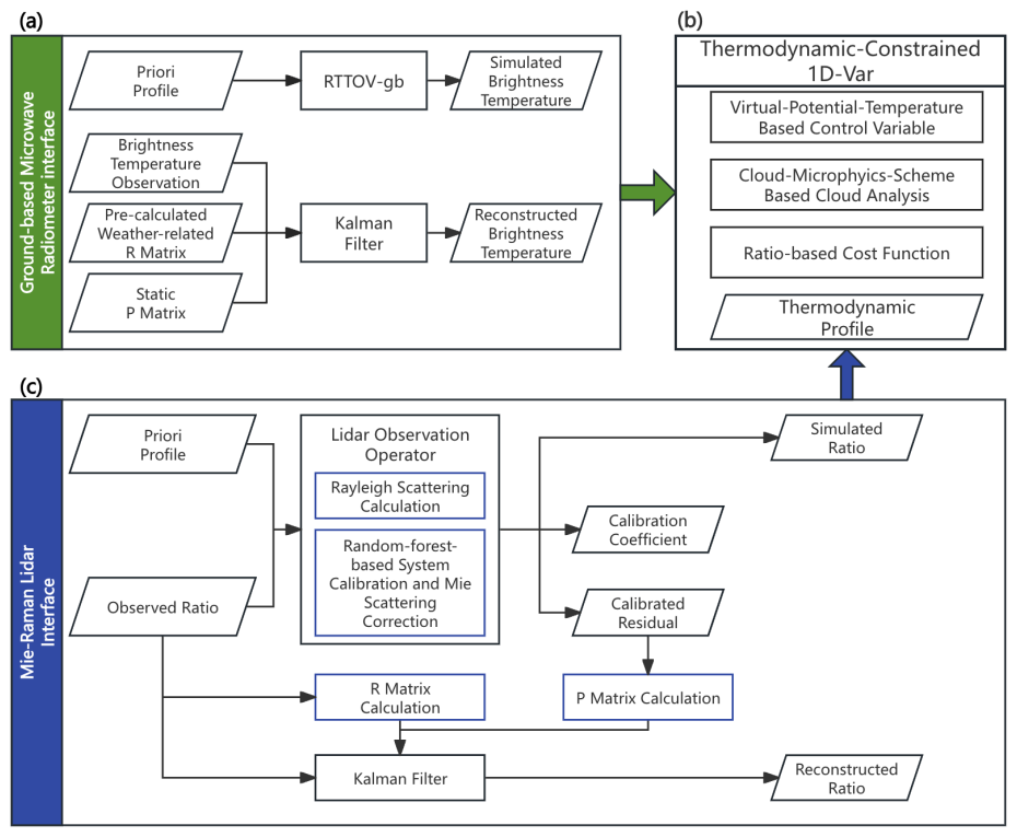
In this study, we retain the core design of the previously developed GMWR-oriented TCKF1D-Var framework (Fig. 2a and b, Zhang et al., 2026b). Specifically, virtual potential temperature (θ_v) is adopted as the control variable, defined as:

$$\begin{array}{}\text{(1)}& {\mathit{\theta }}_{\mathrm{v}}=T{\left({\displaystyle \frac{P_{\mathrm{0}}}{P}}\right)}^{\frac{R_{\mathrm{d}}}{C_{\mathrm{p}}}}\left(\mathrm{1}+\mathrm{0.61}{q}_{\mathrm{v}}-q_{\mathrm{c}}\right),\end{array}$$

where P is air pressure, T is temperature, q_v and q_c are the water vapor and cloud water mixing ratios, respectively, and R_d and C_p are the gas constant and specific heat capacity of dry air at constant pressure. The ratio-based cost function J_(x) is also preserved and expressed as:

$$\begin{array}{}\text{(2)}& J_{\left(x\right)}={\left({\displaystyle \frac{H_{\left(x\right)}}{y}}-\mathrm{1}\right)}^{\mathrm{2}}+{\left({\displaystyle \frac{{\mathit{\theta }}_{\mathrm{v}\left(x\right)}}{{\mathit{\theta }}_{\mathrm{v}\left(x_{\mathrm{o}}\right)}}}-\mathrm{1}\right)}^{\mathrm{2}},\end{array}$$

where y represents the instrument observation at a given time; in this study, it is defined as the ratio of the water vapor Raman signal at 407.5 nm (PR${}_{{\mathrm{H}}_{\mathrm{2}}\mathrm{O}}$) to the nitrogen Raman signal at 386.7 nm (PR${}_{{\mathrm{N}}_{\mathrm{2}}}$). The term x_o denotes the a priori profile, and H_(x) is the lidar observation operator that maps the atmospheric state x to the corresponding simulated observation. The minimization of the cost function is consistently performed using the L-BFGS-B algorithm (Gerber and Furrer, 2019). To enable accurate retrieval of water vapor mass mixing ratio profiles from low single-pulse-energy Raman lidar observations, we introduce two key methodological extensions (Fig. 2c) to the TCKF1D-Var framework. These include (i) the development of a A physics-informed lidar observation operator with random forest calibration (Sect. 2.3.1) for nitrogen and water vapor Raman signals; and (ii) a Kalman filter–based observation fusion strategy with dynamically updated process and observation error covariance matrices (Sect. 2.3.2). Together, these advances substantially enhance the capability of the framework to exploit MRL observations, leading to robust and physically consistent water vapor retrievals.

Figure 2 Workflow of TCKF1D-Var framework.

2.3.1 Lidar observation operator

The lidar observation operator is constructed following the classical Raman lidar formulation described by Ansmann et al. (1992), Whiteman et al. (1992), and Wulfmeyer and Behrendt (2021). The water vapor Raman signal at 407.5 nm can be expressed as

$$\begin{array}{}\text{(3)}& \begin{array}{rl}{\text{PR}}_{{\mathrm{H}}_{\mathrm{2}}\mathrm{O}}& =K_{{\mathrm{H}}_{\mathrm{2}}\mathrm{O}}{\displaystyle \frac{O\left(z\right)}{z^{\mathrm{2}}}}{N}_{{\mathrm{H}}_{\mathrm{2}}\mathrm{O}}\left(z\right){\displaystyle \frac{\mathrm{d}{\mathit{\sigma }}_{{\mathrm{H}}_{\mathrm{2}}\mathrm{O}}\left(\mathit{\pi }\right)}{\mathrm{d}\mathrm{\Omega }}}\\ & \exp \mathit{\{}-{\int }_{\mathrm{0}}^z[{\mathit{\alpha }}_{{\mathrm{H}}_{\mathrm{2}}\mathrm{O}}^{\mathrm{mol}}\left(z\right)+{\mathit{\alpha }}_{{\mathrm{H}}_{\mathrm{2}}\mathrm{O}}^{\mathrm{aer}}\left(z\right)+{\mathit{\alpha }}_{{\mathit{\lambda }}_{\mathrm{0}}}^{\mathrm{mol}}\left(z\right)\\ & +{\mathit{\alpha }}_{{\mathit{\lambda }}_{\mathrm{0}}}^{\mathrm{aer}}\left(z\right)\left]\mathrm{d}z\mathit{\right\}},\end{array}\end{array}$$

where O(z) denotes the overlap function, $K_{{\mathrm{H}}_{\mathrm{2}}\mathrm{O}}$ is the system efficiency factor provided by the instrument manufacturer, and $N_{{\mathrm{H}}_{\mathrm{2}}\mathrm{O}}\left(z\right)$ is the water vapor number density at level z. The term $\frac{\mathrm{d}{\mathit{\sigma }}_{{\mathrm{H}}_{\mathrm{2}}\mathrm{O}}\left(\mathit{\pi }\right)}{\mathrm{d}\mathrm{\Omega }}$ represents the range-independent differential Raman backscatter cross section. The extinction coefficients α^mol(z) and α^aer(z) describe molecular and aerosol extinction at the Raman (407.5 nm) and emitted (354.7 nm) wavelengths, respectively. Similarly, the nitrogen Raman signal at 386.7 nm is given by

$$\begin{array}{}\text{(4)}& \begin{array}{rl}{\text{PR}}_{{\mathrm{N}}_{\mathrm{2}}}& =K_{{\mathrm{N}}_{\mathrm{2}}}{\displaystyle \frac{O\left(z\right)}{z^{\mathrm{2}}}}{N}_{{\mathrm{N}}_{\mathrm{2}}}\left(z\right){\displaystyle \frac{\mathrm{d}{\mathit{\sigma }}_{{\mathrm{N}}_{\mathrm{2}}}\left(\mathit{\pi }\right)}{\mathrm{d}\mathrm{\Omega }}}\\ & \exp \mathit{\{}-{\int }_{\mathrm{0}}^z[{\mathit{\alpha }}_{{\mathrm{N}}_{\mathrm{2}}}^{\mathrm{mol}}\left(z\right)+{\mathit{\alpha }}_{{\mathrm{N}}_{\mathrm{2}}}^{\mathrm{aer}}\left(z\right)+{\mathit{\alpha }}_{{\mathit{\lambda }}_{\mathrm{0}}}^{\mathrm{mol}}\left(z\right)\\ & +{\mathit{\alpha }}_{{\mathit{\lambda }}_{\mathrm{0}}}^{\mathrm{aer}}\left(z\right)\left]\mathrm{d}z\mathit{\right\}},\end{array}\end{array}$$

where $K_{{\mathrm{N}}_{\mathrm{2}}}$ includes all range-independent system parameters for the nitrogen Raman channel, and $N_{{\mathrm{N}}_{\mathrm{2}}}\left(z\right)$ is the nitrogen number density.

Taking the ratio of Eqs. (3) and (4) eliminates common system- and geometry-dependent terms, yielding

$$\begin{array}{}\text{(5)}& \begin{array}{rl}H& ={\displaystyle \frac{{\text{PR}}_{{\mathrm{H}}_{\mathrm{2}}\mathrm{O}}}{{\text{PR}}_{{\mathrm{N}}_{\mathrm{2}}}}}=C_R{\displaystyle \frac{N_{{\mathrm{H}}_{\mathrm{2}}\mathrm{O}}\left(z\right)}{N_{{\mathrm{N}}_{\mathrm{2}}}\left(z\right)}}{\displaystyle \frac{\mathrm{d}{\mathit{\sigma }}_{{\mathrm{H}}_{\mathrm{2}}\mathrm{O}}\left(\mathit{\pi }\right)/\mathrm{d}\mathrm{\Omega }}{\mathrm{d}{\mathit{\sigma }}_{{\mathrm{N}}_{\mathrm{2}}}\left(\mathit{\pi }\right)/d\mathrm{\Omega }}}\\ & {\displaystyle \frac{\exp \left[{\int }_{\mathrm{0}}^z{\mathit{\alpha }}_{{\mathrm{N}}_{\mathrm{2}}}^{\mathrm{mol}}\left(z\right)\mathrm{d}z\right]}{\exp \left[{\int }_{\mathrm{0}}^z{\mathit{\alpha }}_{{\mathrm{H}}_{\mathrm{2}}\mathrm{O}}^{\mathrm{mol}}\left(z\right)\mathrm{d}z\right]}}{\displaystyle \frac{\exp \left[{\int }_{\mathrm{0}}^z{\mathit{\alpha }}_{{\mathrm{N}}_{\mathrm{2}}}^{\mathrm{aer}}\left(z\right)\mathrm{d}z\right]}{\exp \left[{\int }_{\mathrm{0}}^z{\mathit{\alpha }}_{{\mathrm{H}}_{\mathrm{2}}\mathrm{O}}^{\mathrm{aer}}\left(z\right)\mathrm{d}z\right]}},\end{array}\end{array}$$

where C_R = $\frac{K_{{\mathrm{H}}_{\mathrm{2}}\mathrm{O}}}{K_{{\mathrm{N}}_{\mathrm{2}}}}$ is an instrument-dependent constant. The ratio $\frac{N_{{\mathrm{H}}_{\mathrm{2}}\mathrm{O}}\left(z\right)}{N_{{\mathrm{N}}_{\mathrm{2}}}\left(z\right)}$ represents the number density of water vapor molecules relative to that of nitrogen molecules in air. Considering that nitrogen constitutes a nearly constant fraction (78.08 %) of dry air, this ratio can be expressed as

$$\begin{array}{}\text{(6)}& {\displaystyle \frac{N_{{\mathrm{H}}_{\mathrm{2}}\mathrm{O}}\left(z\right)}{N_{{\mathrm{N}}_{\mathrm{2}}}\left(z\right)}}={\displaystyle \frac{m_{{\mathrm{H}}_{\mathrm{2}}\mathrm{O}}/M_{{\mathrm{H}}_{\mathrm{2}}\mathrm{O}}}{\left(m_{\mathrm{air}}/M_{\mathrm{air}}\right)\times \mathrm{0.7808}}},\end{array}$$

where $m_{{\mathrm{H}}_{\mathrm{2}}\mathrm{O}}$ and m_air denote the mass densities of water vapor and dry air, respectively, and $M_{{\mathrm{H}}_{\mathrm{2}}\mathrm{O}}$ = 18.015 g mol⁻¹ and M_air = 28.97 g mol⁻¹ are their corresponding molar masses. The ratio of mass densities can be conveniently expressed in terms of the water vapor mass mixing ratio (qvapor) as

$$\begin{array}{}\text{(7)}& {\displaystyle \frac{m_{{\mathrm{H}}_{\mathrm{2}}\mathrm{O}}}{m_{\mathrm{air}}}}={\displaystyle \frac{\text{qvapor}}{\mathrm{1}-\text{qvapor}}},\end{array}$$

Substituting Eq. (7) into Eq. (6), the molecular number density ratio becomes

$$\begin{array}{}\text{(8)}& \begin{array}{rl}{\displaystyle \frac{N_{{\mathrm{H}}_{\mathrm{2}}\mathrm{O}}\left(z\right)}{N_{{\mathrm{N}}_{\mathrm{2}}}\left(z\right)}}& ={\displaystyle \frac{\text{qvapor}}{\mathrm{1}-\text{qvapor}}}\times {\displaystyle \frac{\mathrm{28.97}\mathrm{g}{\mathrm{mol}}^{-\mathrm{1}}}{\mathrm{18.015}\mathrm{g}{\mathrm{mol}}^{-\mathrm{1}}}}\times {\displaystyle \frac{\mathrm{1}}{\mathrm{0.7808}}}\\ & \approx \mathrm{2.06}{\displaystyle \frac{\text{qvapor}}{\mathrm{1}-\text{qvapor}}}.\end{array}\end{array}$$

The ratio of Raman cross sections $\frac{\mathrm{d}{\mathit{\sigma }}_{{\mathrm{H}}_{\mathrm{2}}\mathrm{O}}\left(\mathit{\pi }\right)/\mathrm{d}\mathrm{\Omega }}{\mathrm{d}{\mathit{\sigma }}_{{\mathrm{N}}_{\mathrm{2}}}\left(\mathit{\pi }\right)/\mathrm{d}\mathrm{\Omega }}$ is assumed constant and set to 1.3 in this study, based on typical values of 6.5 × 10⁻³¹ and 4.8 × 10⁻³¹ cm² sr⁻¹ for water vapor and nitrogen, respectively. The molecular extinction term is parameterized as

$$\begin{array}{}\text{(9)}& {\mathit{\alpha }}_{\mathit{\lambda }}^{\mathrm{mol}}={\mathit{\alpha }}_{\mathit{\lambda },\mathrm{std}}^{\mathrm{mol}}{\displaystyle \frac{P\left(z\right)}{P_{\mathrm{0}}}}{\displaystyle \frac{T_{\mathrm{0}}}{T\left(z\right)}},\end{array}$$

where ${\mathit{\alpha }}_{\mathit{\lambda },\mathrm{std}}^{\mathrm{mol}}$ is the standard-atmosphere extinction coefficient. P₀ = 101 325 Pa and T₀ = 288.15 K represent the reference air pressure and temperature of the standard atmosphere, respectively. In this study, values of 7.0 × 10⁻⁵ and 6.0 × 10⁻⁵ m⁻¹ are used for 386.7 and 407.5 nm, respectively. This leads to

$$\begin{array}{}\text{(10)}& {\displaystyle \frac{\exp \left[{\int }_{\mathrm{0}}^z{\mathit{\alpha }}_{{\mathrm{N}}_{\mathrm{2}}}^{\mathrm{mol}}\left(z\right)\mathrm{d}z\right]}{\exp \left[{\int }_{\mathrm{0}}^z{\mathit{\alpha }}_{{\mathrm{H}}_{\mathrm{2}}\mathrm{O}}^{\mathrm{mol}}\left(z\right)\mathrm{d}z\right]}}=\exp \left[{\mathrm{10}}^{-\mathrm{5}}{\int }_{\mathrm{0}}^z{\displaystyle \frac{P\left(z\right)}{P_{\mathrm{0}}}}{\displaystyle \frac{T_{\mathrm{0}}}{T\left(z\right)}}\mathrm{d}z\right].\end{array}$$

The aerosol extinction term is parameterized using the Ångström power law (Ångström, 1929):

$$\begin{array}{}\text{(11)}& {\mathit{\alpha }}_{\mathit{\lambda }}^{\mathrm{aer}}={\mathit{\alpha }}_{\mathrm{355}}^{\mathrm{aer}}{\left({\displaystyle \frac{\mathit{\lambda }}{\mathrm{355.0}}}\right)}^{-A},\end{array}$$

where A is the Ångström exponent derived from 354.7 and 532 nm aerosol extinction measurements:

$$\begin{array}{}\text{(12)}& A=-{\displaystyle \frac{\ln \left(\frac{{\mathit{\alpha }}_{\mathrm{355}}^{\mathrm{aer}}}{{\mathit{\alpha }}_{\mathrm{532}}^{\mathrm{aer}}}\right)}{\ln \left(\frac{\mathrm{355.0}}{\mathrm{532.0}}\right)}},\end{array}$$

Thus, the aerosol contribution becomes

$$\begin{array}{}\text{(13)}& \begin{array}{rl}& {\displaystyle \frac{\exp \left[{\int }_{\mathrm{0}}^z{\mathit{\alpha }}_{{\mathrm{N}}_{\mathrm{2}}}^{\mathrm{aer}}\left(z\right)\mathrm{d}z\right]}{\exp \left[{\int }_{\mathrm{0}}^z{\mathit{\alpha }}_{{\mathrm{H}}_{\mathrm{2}}\mathrm{O}}^{\mathrm{aer}}\left(z\right)\mathrm{d}z\right]}}\\ & =\exp \left\{{\mathit{\alpha }}_{\mathrm{355}}^{\mathrm{aer}}{\int }_{\mathrm{0}}^z\left[{\left({\displaystyle \frac{\mathrm{386.7}}{\mathrm{355.0}}}\right)}^{-A}-{\left({\displaystyle \frac{\mathrm{407.5}}{\mathrm{355.0}}}\right)}^{-A}\right]\mathrm{d}z\right\},\end{array}\end{array}$$

Substituting Eqs. (8), (10), and (13) into Eq. (5), the final lidar observation operator is obtained as

$$\begin{array}{}\text{(14)}& \begin{array}{rl}& H=\mathrm{2.68}\times C_R\cdot {\displaystyle \frac{\text{qvapor}}{\mathrm{1}-\text{qvapor}}}\\ & \cdot \exp \mathit{\{}{\mathrm{10}}^{-\mathrm{5}}{\int }_{\mathrm{0}}^z{\displaystyle \frac{P\left(z\right)}{P_{\mathrm{0}}}}{\displaystyle \frac{T_{\mathrm{0}}}{T\left(z\right)}}\mathrm{d}z\\ & +{\mathit{\alpha }}_{\mathrm{355}}^{\mathrm{aer}}{\int }_{\mathrm{0}}^z\left[{\left({\displaystyle \frac{\mathrm{386.7}}{\mathrm{355.0}}}\right)}^{-A}-{\left({\displaystyle \frac{\mathrm{407.5}}{\mathrm{355.0}}}\right)}^{-A}\right]\mathrm{d}z\mathit{\}},\end{array}\end{array}$$

which depends only on instrument constants and directly observed quantities. The coefficient 2.68 results from the combination of the molecular number density ratio (Eq. 8) and the assumed Raman cross-section ratio.

Although the C_R in Eq. (14) can, in principle, be determined from factory-calibrated system constants, such an approach is not suitable for long-term observations. Continuous operation of the MRL system leads to gradual degradation in optical efficiency, resulting in inconsistencies between the initial calibration constants and the actual instrument state. Consequently, the direct use of factory-derived C_R introduces systematic biases in the retrieved thermodynamic profiles. In addition, the aerosol extinction coefficient at 355 nm provided by the MRL has a temporal resolution of 5 min, which is coarser than the 1 min resolution of the nitrogen and water vapor Raman signals. Incorporating this lower-resolution product into the Mie scattering term in Eq. (14) may degrade retrieval accuracy, particularly under rapidly evolving atmospheric conditions. To address these limitations, a random forest (Belgiu and Drăguţ, 2016) based calibration strategy is introduced to account for the combined effects of the system calibration coefficient and unresolved aerosol extinction-related uncertainties. The random forest model is trained using lidar-observed Raman signals within a moving temporal window preceding the retrieval time, and no external thermodynamic observations (e.g., radiosonde data) are used in the training process, thereby avoiding potential information leakage in the validation. The modified observation operator can thus be expressed as

$$\begin{array}{}\text{(15)}& \begin{array}{rl}H& =\mathrm{2.68}{\displaystyle \frac{\text{qvapor}}{\mathrm{1}-\text{qvapor}}}\cdot \exp \left\{{\mathrm{10}}^{-\mathrm{5}}\underset{\mathrm{0}}{\overset{z}{\int }}{\displaystyle \frac{P\left(z\right)}{P_{\mathrm{0}}}}{\displaystyle \frac{T_{\mathrm{0}}}{T\left(z\right)}}\mathrm{d}z\right\}\\ & \cdot \mathtt{\text{RandomForest}}\left(y\right),\end{array}\end{array}$$

where RandomForest denotes the random forest model with 100 trees and a squared-error split criterion, and is applied independently at each vertical level using time-series features derived from the Raman signal ratio within the temporal window. It should be emphasized that the random forest component serves only as a multiplicative correction to the physically derived operator, rather than replacing its underlying physical structure. In this way, the physical interpretability of the observation operator is preserved while improving its adaptability to time-varying instrument performance and atmospheric conditions.

At this stage, the lidar observation operator is established. In addition to providing the simulated ratio (y_sim) derived from the atmospheric state profiles, the operator also outputs a calibration coefficient (Coef_Cal) profile and calibrated residual (Res_Cal) profiles, thereby enabling a comprehensive characterization of the forward-model uncertainty. Specifically, the Coef_Cal profile represents the combined term $C_R\cdot \exp \left\{{\mathit{\alpha }}_{\mathrm{355}}^{\mathrm{aer}}{\int }_{\mathrm{0}}^z\left[{\left(\frac{\mathrm{386.7}}{\mathrm{355.0}}\right)}^{-A}-{\left(\frac{\mathrm{407.5}}{\mathrm{355.0}}\right)}^{-A}\right]\mathrm{d}z\right\}$ in Eq. (14), which is estimated using the random forest algorithm constrained by the MRL Raman channel observations. Meanwhile, the Res_Cal profiles is defined as the difference between the MRL-observed ratio and the simulated ratio within a time window preceding the thermodynamic profile retrieval time. This residual quantifies the discrepancy between observations and the operator-simulated signal given the atmospheric state, and is therefore interpreted as the process error of the lidar observation operator.

2.3.2 Kalman filter–based observation fusion

Kalman filtering provides a recursive Bayesian framework for optimally combining model predictions and observations under uncertainty (Kalman, 1960). By explicitly accounting for process and observation errors through their respective covariance matrices, it enables sequential updating of the system state while minimizing estimation variance. One of its key advantages lies in its ability to handle noisy and incomplete measurements, while maintaining temporal consistency in the retrieved variables. In addition, the Kalman filter naturally incorporates prior information and propagates uncertainty forward in time, making it suitable for retrieving atmospheric thermodynamic profile low-single-pulse-energy MRL observation where both measurement noise and model errors are non-negligible. Consequently, dynamically updating the process error covariance (P) matrix and the observation error covariance (R) matrix becomes essential. For low-single-pulse-energy MRL Raman channel observations, both error sources exhibit strong temporal variability: the R is influenced by rapidly changing measurement uncertainty associated with environmental contamination and signal attenuation, while the P reflects model inadequacies that vary with atmospheric conditions and the performance of the lidar observation operator. Therefore, by dynamically estimating and updating both covariance matrices, the Kalman filter can more accurately represent the time-dependent error structure, thereby improving the reliability and physical consistency of the fused atmospheric state estimates.

In this study, the R matrix is estimated using the variability of the MRL-observed ratio relative to its short-term mean within a time window preceding the thermodynamic profile retrieval time. Specifically, the deviations between the instantaneous ratio (y) and its temporal mean over this period ($\stackrel{\mathrm{‾}}{y}$) are used to quantify the observation uncertainty as

$$\begin{array}{}\text{(16)}& \mathbf{R}={\displaystyle \frac{{\left(y-\stackrel{\mathrm{‾}}{y}\right)}^T\cdot \left(y-y\right)}{N_{\mathrm{obs}}}},\end{array}$$

where the superscript T denotes the transpose operator, and N_obs represents the number of MRL Raman channel observations within a time window prior to the retrieval. The P matrix is estimated using an analogous formulation but based on the Res_Cal derived from the lidar observation operator, computed as

$$\begin{array}{}\text{(17)}& \mathbf{P}={\displaystyle \frac{{\text{Res}}_{\mathrm{Cal}}^T\cdot {\text{Res}}_{\mathrm{Cal}}}{N_{\mathrm{obs}}}}.\end{array}$$

In this study, both the diagonal and off-diagonal elements of the R and P matrices are retained to account for vertical error correlations associated with turbulent mixing within the boundary layer, which are expected to influence the structure of the retrieved water vapor mass mixing ratio profiles (Foken et al., 2012). To provide further insight into the diagnosed error covariance characteristics, Appendix A presents representative R and P matrices (Figs. A1 and A2) derived from all precipitation cases used in this study, including a comparison of their vertical correlation structures under different precipitation intensity categories.

3 Results and discussion

3.1 Sensitivity of Retrieval Performance to Temporal Resolution

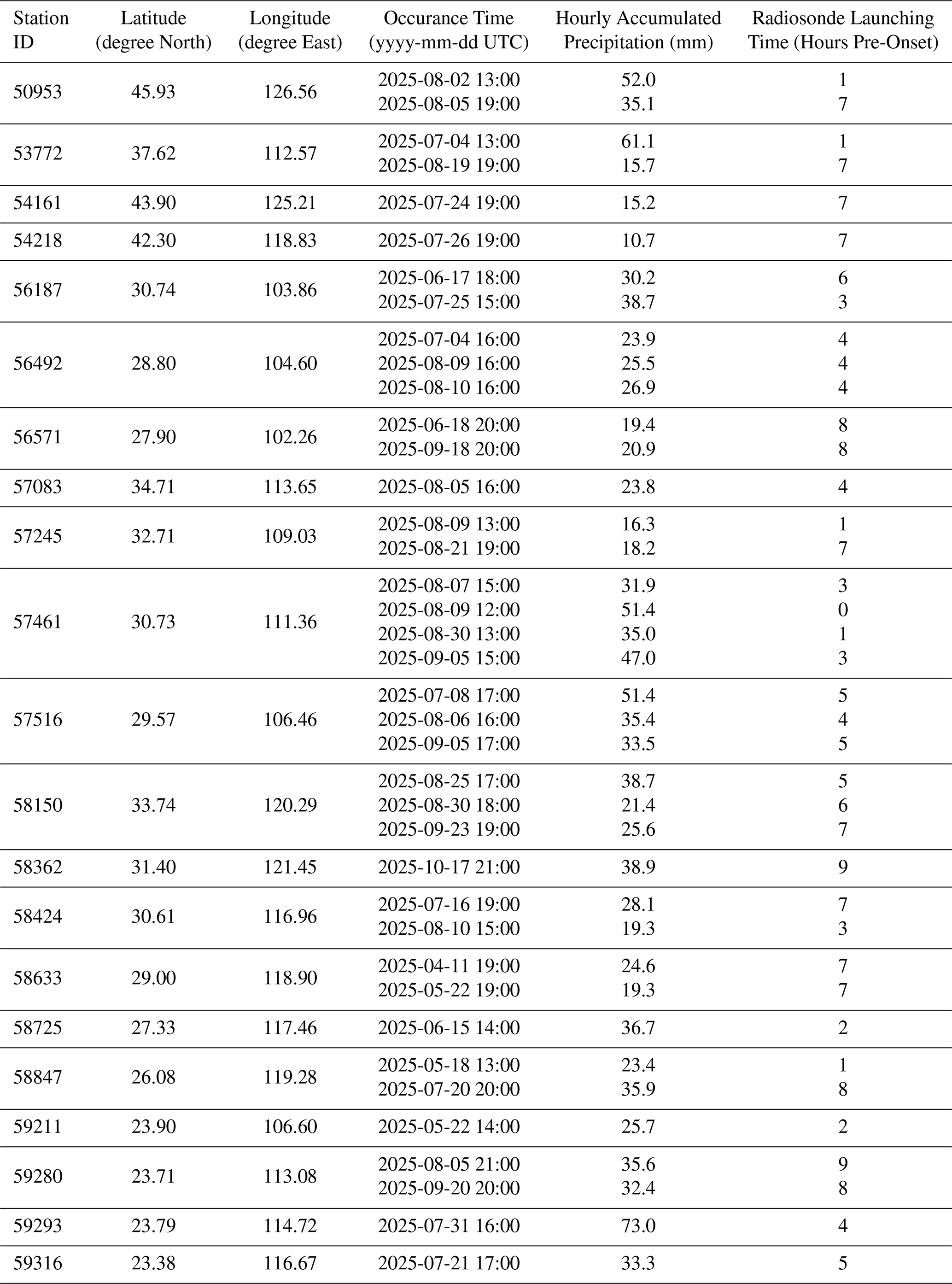
Previous studies (Laly et al., 2024; Laly and Chazette, 2025) have suggested that the temporal resolution for water vapor mass mixing ratio profile retrieval using the 407.5 and 386.7 nm Raman channels typically ranges from 15 to 30 min. However, owing to differences in instrumental configurations and retrieval strategies, the optimal temporal resolution adopted in this study cannot be directly prescribed and must instead be determined through sensitivity experiments based on representative cases. Given that this study focuses on the evolution of boundary-layer water vapor prior to the initiation of short-duration intense nocturnal precipitation, radiosonde observations at 12:00 UTC preceding the triggering time are selected as the reference. Corresponding water vapor mass mixing ratio profiles with temporal resolutions of 10, 20, and 30 min are constructed from MRL observations, and their performance is evaluated using the mean bias (MB) and root mean squared error (RMSE), defined as MB = $\stackrel{\mathrm{‾}}{\left(\text{radiosonde}-\text{retrieval}\right)}$ and RMSE = $\sqrt{{\stackrel{\mathrm{‾}}{\left(\text{radiosnonde}-\text{retrieval}\right)}}^{\mathrm{2}}}$, respectively, as the primary metrics to identify the temporal resolution most suitable for the MRL observations and the TCKF1D-Var framework. Furthermore, based on hourly accumulated precipitation observations co-located with 56 radiosonde stations in 2025, heavy precipitation events at each station are identified using the 99th percentile of the station-specific annual hourly precipitation distribution as the threshold. Nighttime extreme precipitation events are then selected from these events by restricting to periods with a solar elevation angle lower than −6°. The selected 39 cases, including station locations, occurrence times, and hourly rainfall intensity, are summarized in Table 2.

Table 2 Summary of the selected case studies used for the sensitivity experiments.

The mean error profiles derived from the sensitivity experiments (Fig. 3a) indicate a clear dependence of retrieval performance on the chosen temporal resolution within the TCKF1D-Var framework. Among the tested configurations, the 30 min temporal resolution (purple) yields the smallest MB, followed by the 20 min configuration (green), while the 10 min resolution (red) exhibits the largest MB. Despite these differences, all three experiments show consistently lower mean errors than the ERA5 prior profile (black), demonstrating the capability of the proposed framework to effectively improve water vapor mass mixing ratio retrievals. Consistent behavior is also observed in the RMSE profiles (Fig. 3b), where the measurement uncertainty associated with the 30 min temporal resolution (purple) is significantly reduced compared to those obtained with 20 min (green), 10 min (red), and the ERA5 prior (black). This suggests that extending the temporal averaging window enhances the water vapor information content and leads to more stable retrievals. Considering both the mean error and measurement uncertainty, a 30 min time window preceding the thermodynamic profile retrieval time is therefore selected as the optimal configuration for the TCKF1D-Var framework in this study.

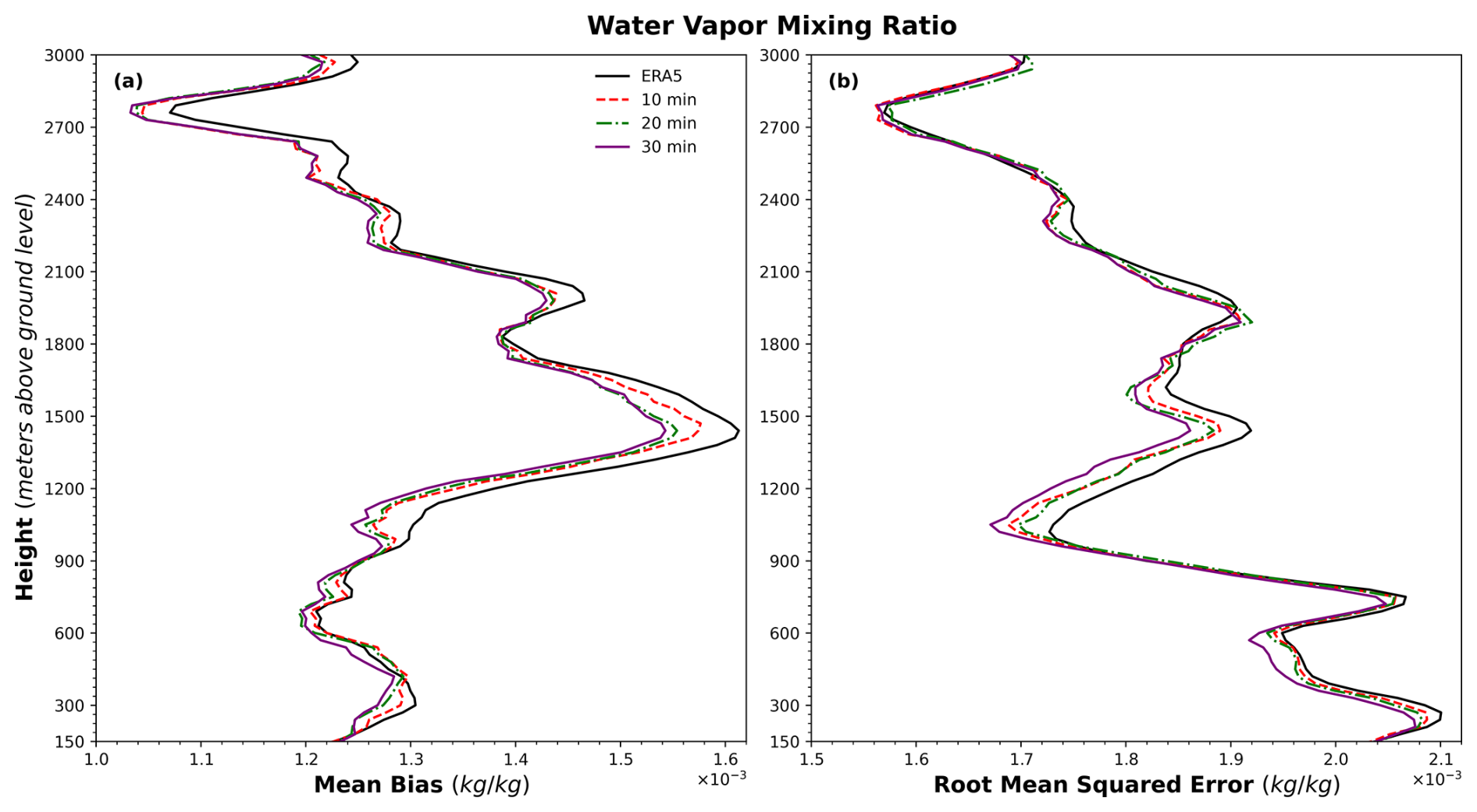
Figure 3 Vertical profiles of (a) mean bias (MB) and (b) root mean square error (RMSE) of the retrieved water vapor mass mixing ratio profiles obtained from the sensitivity experiments with temporal resolutions of 10 min (red), 20 min (green), and 30 min (purple), together with the ERA5 prior profile (black). The 30 min configuration yields the smallest MB and RMSE, followed by the 20 and 10 min configurations, while all experiments show improved performance compared to the ERA5 prior.

To assess why the 30 min temporal resolution yields the highest retrieval accuracy, we examine the relative magnitude of the effective observational information provided by the observations and the forward model error by introducing the innovation-to-forward model error ratio (IFR), defined as the ratio between the innovation and the observation operator error:

$$\begin{array}{}\text{(18)}& \text{IFR}={\displaystyle \frac{\text{Innovation}}{{\text{Error}}_{\mathrm{Operator}}}},\end{array}$$

where the Innovation is defined as the difference between the reconstructed ratio obtained from MRL observations using the Kalman filter (Ratio${}_{\mathrm{obs}}^{\mathrm{reconstruct}}$) and the simulated ratio derived from the lidar observation operator driven by the ERA5 prior profile (Ratio${}_{\mathrm{sim}}^{\mathrm{ERA}\mathrm{5}}$):

$$\begin{array}{}\text{(19)}& \text{Innovation}=\left|{\text{Ratio}}_{\mathrm{obs}}^{\mathrm{reconstruct}}-{\text{Ratio}}_{\mathrm{sim}}^{\mathrm{ERA}\mathrm{5}}\right|,\end{array}$$

This term represents the mismatch between the prior-driven forward simulation and the observation-constrained reconstruction, and thus reflects the information gain introduced by the observations. The observation operator error (Error_Operator) is defined as the difference between the reconstructed ratio (Ratio${}_{\mathrm{obs}}^{\mathrm{reconstruct}}$) and the simulated ratio obtained using radiosonde profiles (Ratio${}_{\mathrm{sim}}^{\mathrm{Radiosonde}}$):

$$\begin{array}{}\text{(20)}& {\text{Error}}_{\mathrm{Operator}}=\left|{\text{Ratio}}_{\mathrm{obs}}^{\mathrm{reconstruct}}-{\text{Ratio}}_{\mathrm{sim}}^{\mathrm{Radiosonde}}\right|,\end{array}$$

This quantity characterizes the discrepancy between the forward model simulation based on the best-available atmospheric state (radiosonde observations) and the reconstructed observation, thereby providing a measure of the forward model (observation operator) uncertainty. Based on these definitions, an IFR value greater than 1.0 indicates that the effective observational information exceeds the forward model error, suggesting that the observational signal is relatively strong compared to forward model uncertainties. Conversely, IFR values smaller than 1.0 indicate that the observational signal may be more strongly affected by forward model uncertainties, limiting the ability of the assimilation system to effectively adjust the prior profile. It should be noted that the IFR defined in this study is a diagnostic quantity that is inherently framework-dependent within the TCKF1D-Var system, rather than a rigorous information-theoretic measure. It does not represent formal information content in the sense of information theory, and therefore should not be interpreted as directly quantifying absolute information gain. Instead, the IFR is introduced as a qualitative indicator to describe the relative magnitude between observational constraints and forward model uncertainty, thereby providing a consistent basis for comparing different experimental configurations within the same retrieval framework. Accordingly, the interpretation of the IFR throughout this study is intentionally limited to comparative and diagnostic purposes, rather than quantitative assessment of information content. Care should therefore be taken when generalizing this metric beyond the specific retrieval system used in this work.

The vertical distributions of IFR averaged over the cases listed in Table 2 are presented in Fig. 4 for the three sensitivity experiments with temporal resolutions of 10, 20, and 30 min. It is evident that the IFR profile associated with the 30 min configuration (purple) is generally higher than those of the 20 min (green) and 10 min (red) configurations. This indicates that the superior accuracy of the 30 min retrievals can be attributed to a more favorable balance between observational information and forward model error. Specifically, the longer Kalman filter time window enhances the reconstructed ratio, leading to larger innovations relative to the ERA5-based prior simulation. As a result, the observational information becomes less susceptible to being obscured by the noise of the lidar observation operator, thereby improving the overall retrieval performance. It should be noted, however, that the above analysis is limited to explaining why the 30 min temporal resolution outperforms the 10 and 20 min configurations, and does not imply a monotonic improvement of retrieval accuracy with increasing Kalman filter window length. Although further increases in the temporal window may potentially enhance retrieval accuracy, they may simultaneously reduce the capability to capture rapid atmospheric variations within the boundary layer preceding the onset of intense precipitation. This trade-off could ultimately degrade the performance of the TCKF1D-Var method in short-term severe weather early warning applications.

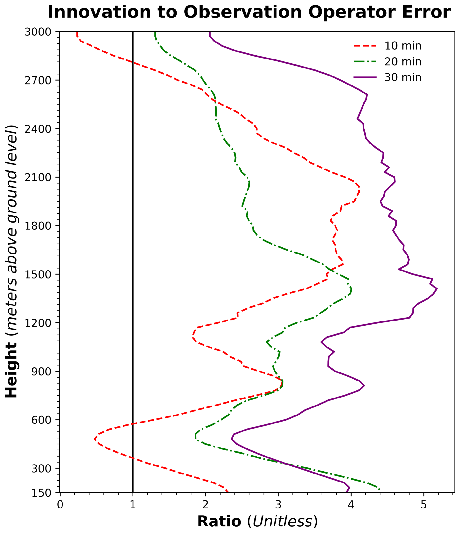
Figure 4 Vertical distributions of the mean innovation-to-observation operator error ratio (IFR) for the three sensitivity experiments with temporal resolutions of 10 min (red), 20 min (green), and 30 min (purple), averaged over the cases listed in Table 2. The IFR quantifies the relative magnitude of effective observational information with respect to forward model error. Values greater than 1.0 (black) indicate that the observational information dominates over the forward model uncertainty, whereas values smaller than 1.0 suggest that the information content is largely obscured by forward model errors.

3.2 Evaluation of Retrieved Thermodynamic Profiles

According to the statistics summarized in Table 2, the lower bound of nighttime extreme precipitation occurring at the 56 MRL-radiosonde co-located stations in 2025 is 10.7 mm. Therefore, a threshold of hourly accumulated precipitation exceeding 10 mm during nighttime is adopted to define heavy precipitation events, allowing for an expanded sample set and a more general evaluation. The statistical distribution of the enlarged samples is presented in Table 3. In the subsequent analyses, the selected events are further classified into three precipitation-intensity categories according to the hourly accumulated precipitation: 10–20, 20–30, and ≥ 30 mm. For events with hourly precipitation of 10–20 mm and those exceeding 30 mm, the lead-time between the 12:00 UTC radiosonde launches and the heavy precipitation onset time ranges from 0 to 9 h. In contrast, for events with precipitation between 20 and 30 mm, this time difference ranges from 0 to 8 h. The number of events within the 10–20 mm category (170 cases) is substantially larger than those in the 20–30 mm (28 cases) and ≥ 30 mm (26 cases) categories. Applying the same evaluation approach described in Sect. 3.1 to the selected cases in Table 3, the vertical distributions of the MB with 95 % confidence intervals (Fig. 5a) and the RMSE (Fig. 5b) are obtained for the TCKF1D-Var water vapor mass mixing ratio profiles with a temporal resolution of 30 min, as well as for the ERA5 prior profiles. Consistent with the results shown in Fig. 3, the evaluation based on the expanded sample set further confirms that the TCKF1D-Var retrievals exhibit lower MB and RMSE than the ERA5 prior profiles. This demonstrates that, at a temporal resolution of 30 min, the TCKF1D-Var framework, constrained by MRL Raman channel observations, has a clear capability to improve the ERA5 prior water vapor mass mixing ratio profiles. In addition, the results based on the expanded samples indicate that the improvement in water vapor mass mixing ratio retrieval is more pronounced within the 1200–3000 m altitude above ground level compared to below 1200 m. This feature is broadly consistent with the findings in Fig. 3, although the altitude separating the two regimes (previously around 1050 m in Fig. 3) shows a slight upward shift in the present analysis.

Table 3 Statistical distribution of the expanded sample set of nighttime heavy precipitation events.

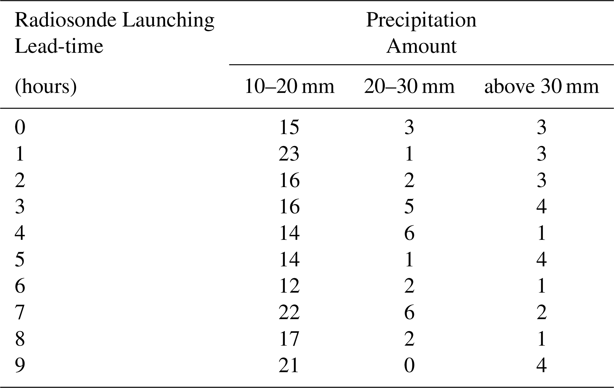
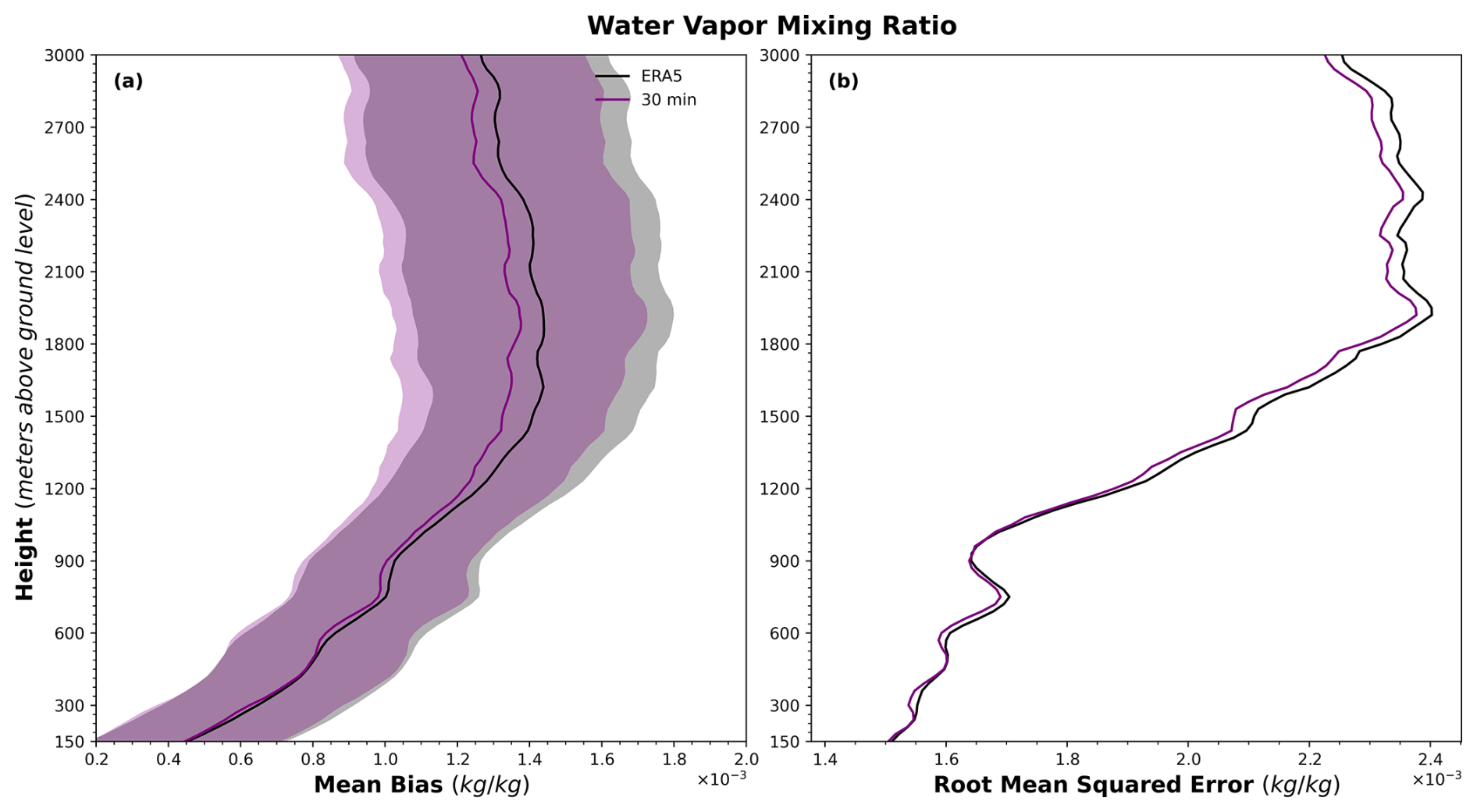
Figure 5 Vertical distributions of (a) mean bias with 95 % confidence intervals and (b) root-mean-square error (RMSE) for water vapor mass mixing ratio profiles derived from the TCKF1D-Var method with a temporal resolution of 30 min (purple) and from ERA5 prior profiles (black), based on the expanded sample set of nighttime heavy precipitation events defined in Table 3. The shaded areas represent the 95 % confidence intervals.

To investigate the dependence of retrieval accuracy on precipitation intensity, the MB with 95 % confidence intervals and RMSE profiles are calculated separately for three categories of nighttime heavy precipitation events defined in Table 3. For the 10–20 mm category, the resulting MB (Fig. 6a) and RMSE (Fig. 6b) are highly consistent with those obtained from the full sample (Fig. 5). This similarity is primarily attributed to the dominance of this category, which accounts for approximately 75.8 % of the total sample size. In contrast, the results for the 20–30 mm category show more pronounced differences compared to the full-sample statistics. Specifically, while the full-sample MB exhibits a vertical structure characterized by lower values near the surface (approximately 0.55 × 10⁻³ kg kg⁻¹) and higher values aloft (approximately 1.4 × 10⁻³ kg kg⁻¹), the 20–30 mm category displays a more vertically uniform distribution (Fig. 6c), with mean bias values generally ranging between 1.5 × 10⁻³ and 2.3 × 10⁻³ kg kg⁻¹. Similarly, the RMSE for the full sample increases with height (from 1.5 × 10⁻³ to 2.35 × 10⁻³ kg kg⁻¹), whereas the 20–30 mm category (Fig. 6d) shows values between 2.0 × 10⁻³ and 2.75 × 10⁻³ kg kg⁻¹, with a notable reduction in RMSE within the 900–1200 m layer. The most distinct differences are observed for the ≥ 30 mm category. The characteristic vertical pattern of MB observed in the full sample (lower near the surface and higher aloft) disappears entirely (Fig. 6e). Moreover, the 95 % confidence intervals are broader than those of the full sample and exhibit an opposite vertical tendency, with larger uncertainties near the surface and smaller ones at higher altitudes. In addition, a reversal is found in the RMSE vertical structure (Fig. 6f), which changes from increasing with height (in the full sample) to decreasing with height for the ≥ 30 mm category. Despite these substantial differences across precipitation intensity classes, the overall conclusion remains robust: the TCKF1D-Var water vapor mass mixing ratio profiles with a temporal resolution of 30 min consistently outperform the ERA5 prior profiles in terms of both MB and RMSE.

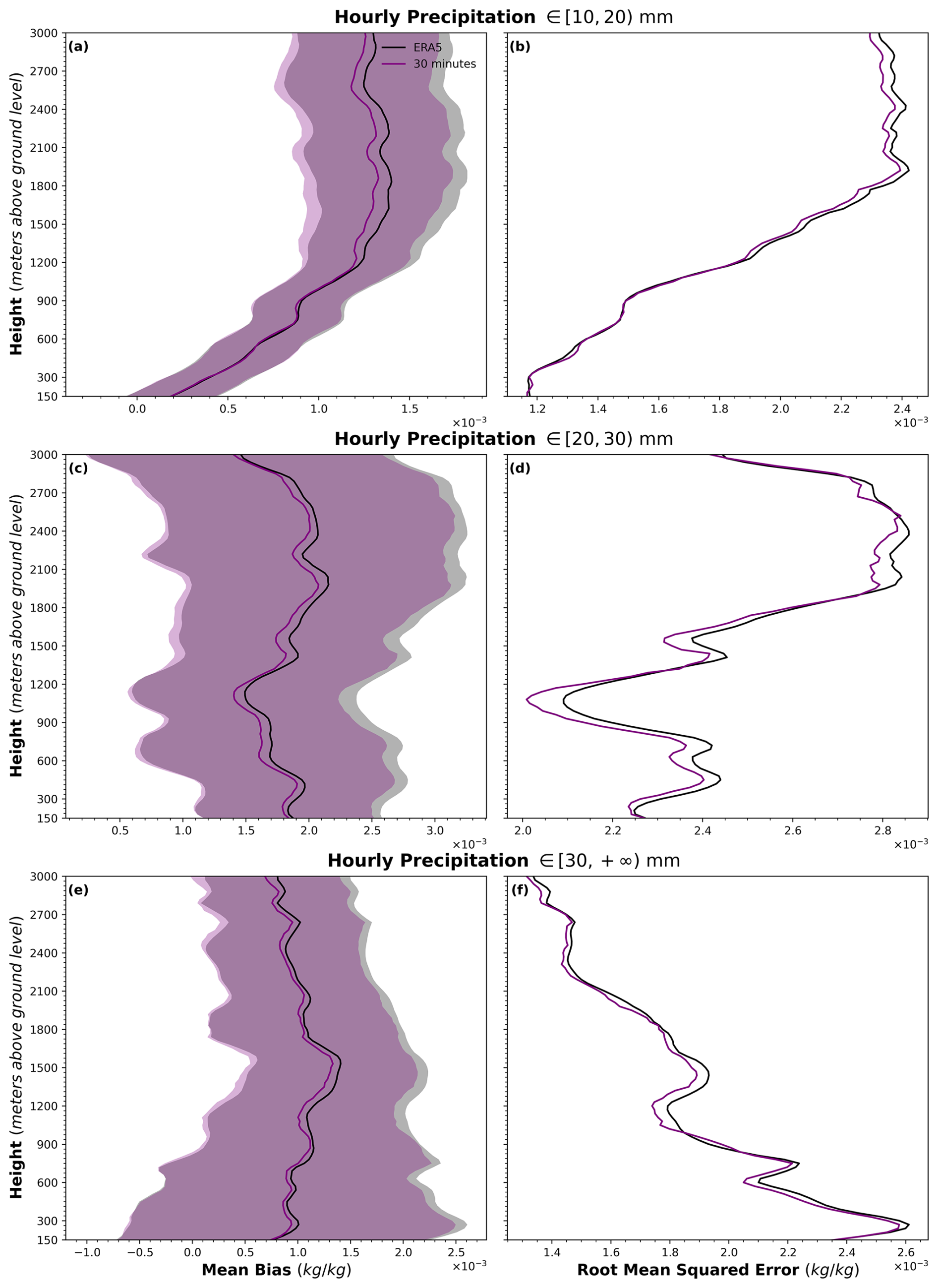
Figure 6 Vertical distributions of mean bias with 95 % confidence intervals (a, c, e) and root mean squared error (b, d, f) for water vapor mass mixing ratio profiles derived from the TCKF1D-Var method with a temporal resolution of 30 min and from ERA5 prior profiles, stratified by precipitation intensity: (a, b) 10–20 mm, (c, d) 20–30 mm, and (e, f) ≥ 30 mm. The shaded areas represent the 95 % confidence intervals.

Based on the results presented in Figs. 3a, 5a, and 6a, c, e, it is evident that the TCKF1D-Var method, constrained by MRL Raman channel observations, can correct the overall dry bias of the ERA5 prior water vapor mass mixing ratio profiles within the 0–3000 m layer preceding nighttime heavy precipitation events. However, the relationship between the retrieved water vapor mass mixing ratio profile's analysis increment and the lead time relative to precipitation onset remains to be clarified. However, it should be noted that the interpretation of the retrieved moistening signal requires caution, as part of the analysis increment may also represent corrections of potential ERA5 prior biases under convective boundary-layer conditions, rather than solely independent evidence of atmospheric moisture evolution. In this context, the increments should be interpreted primarily as retrieval-based adjustments relative to the prior state, rather than direct observational confirmation of physical moisture tendencies. To further examine the temporal behavior of the analysis increments, the time–height evolution of the mean analysis increment (Fig. 7), defined as the difference between the TCKF1D-Var retrievals and the ERA5 prior profiles, is calculated using the cases summarized in Table 3. As shown in Fig. 7, within the 1200–3000 m above ground level, the mean analysis increment remains consistently positive throughout the 0–9 h period prior to precipitation onset, indicating a persistent moistening correction to the ERA5 prior. Moreover, as the observation time approaches the onset of heavy precipitation, the magnitude of the analysis increment increases progressively, reaching a pronounced maximum within 2 h before the onset, with values exceeding 1.0 × 10⁻⁴ kg kg⁻¹. In the 750–1200 m layer, the temporal evolution of the analysis increment exhibits a more complex structure. The increment is positive at lead times earlier than 7 h, becomes negative between 7 and 3 h, and turns positive again during the final 3 h before precipitation onset. The magnitude in this layer ranges between −0.25 × 10⁻⁴ and 0.25 × 10⁻⁴ kg kg⁻¹, which is notably smaller than that in the 1200–3000 m layer. below 750 m, the magnitude of the analysis increment is comparable to that within the 750–1200 m layer, but with a distinct temporal pattern: analysis increment remains positive from 9 to 2 h before precipitation onset and becomes negative during the last 2 h. These results indicate that the analysis increments introduced by the TCKF1D-Var method, which reflect the contribution of MRL Raman channel observations, exhibit clear temporal and vertical variability prior to heavy precipitation onset. Both the magnitude and vertical structure of the analysis increments reach their most pronounced state within approximately 2 h before the onset of heavy precipitation.

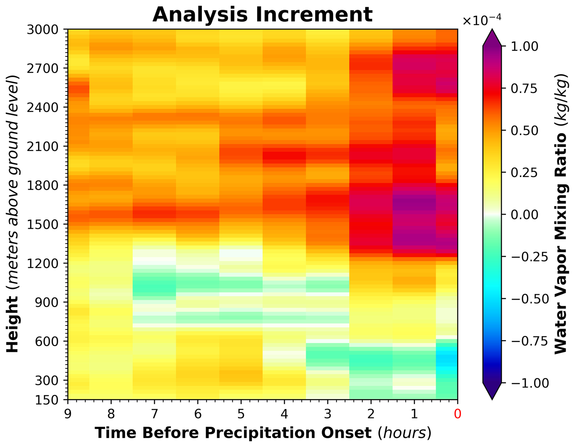
Figure 7 Time–height evolution of the mean analysis increment of water vapor mass mixing ratio profiles, defined as the difference between the TCKF1D-Var retrievals (30 min temporal resolution) and the ERA5 prior profiles. The red-colored x-axis tick label (0 h) denotes the precipitation occurrence time.

3.3 Observed nocturnal boundary-layer moisture evolution prior to precipitation onset

Although the statistical results presented in Sect. 3.2 reveal clear temporal and vertical variability in the analysis increments prior to nocturnal heavy precipitation, representative case studies are still necessary to determine whether these characteristics can also be identified in individual events. Therefore, three representative nocturnal heavy precipitation cases were selected for detailed analysis, corresponding to the maximum (Fig. 8), minimum (Fig. 9), and median-like (Fig. 10) hourly accumulated precipitation intensities. The TCKF1D-Var retrieved water vapor mass mixing ratio profiles were compared with the ERA5 prior profiles to further evaluate the performance of the proposed method under different precipitation intensity conditions.

The maximum hourly rainfall case occurred at station 59293 at 16:00 UTC on 31 July 2025, with an hourly accumulated precipitation amount of 73.0 mm. Comparison of the TCKF1D-Var retrieved water vapor mass mixing ratio profiles at 30 min temporal resolution (Fig. 8a) with the ERA5 prior profiles (Fig. 8b) reveals pronounced analysis increments, particularly within the 0–1500 m layer during the 2 h preceding precipitation onset. Relative to ERA5, the TCKF1D-Var retrievals provide a more detailed depiction of upward moisture transport below 750 m and enhanced temporal variability within the 750–1500 m layer prior to precipitation. The evolution of the Innovation (Fig. 8c) and reconstructed observations (Fig. 8d) further supports these features. As precipitation onset approaches, both the magnitude and vertical variability of the reconstructed observations increase substantially, exhibiting temporal–vertical structures consistent with those shown in Figs. 8a and b. This agreement indicates that the reconstructed observations derived from the MRL Raman channel measurements within the Kalman filtering framework are sensitive to the evolution of atmospheric moisture structures within the 0–3000 m layer prior to nocturnal heavy precipitation. In addition, the consistency between the Innovation patterns and the corresponding moisture structures further supports the reliability of the observation operator used in this study.

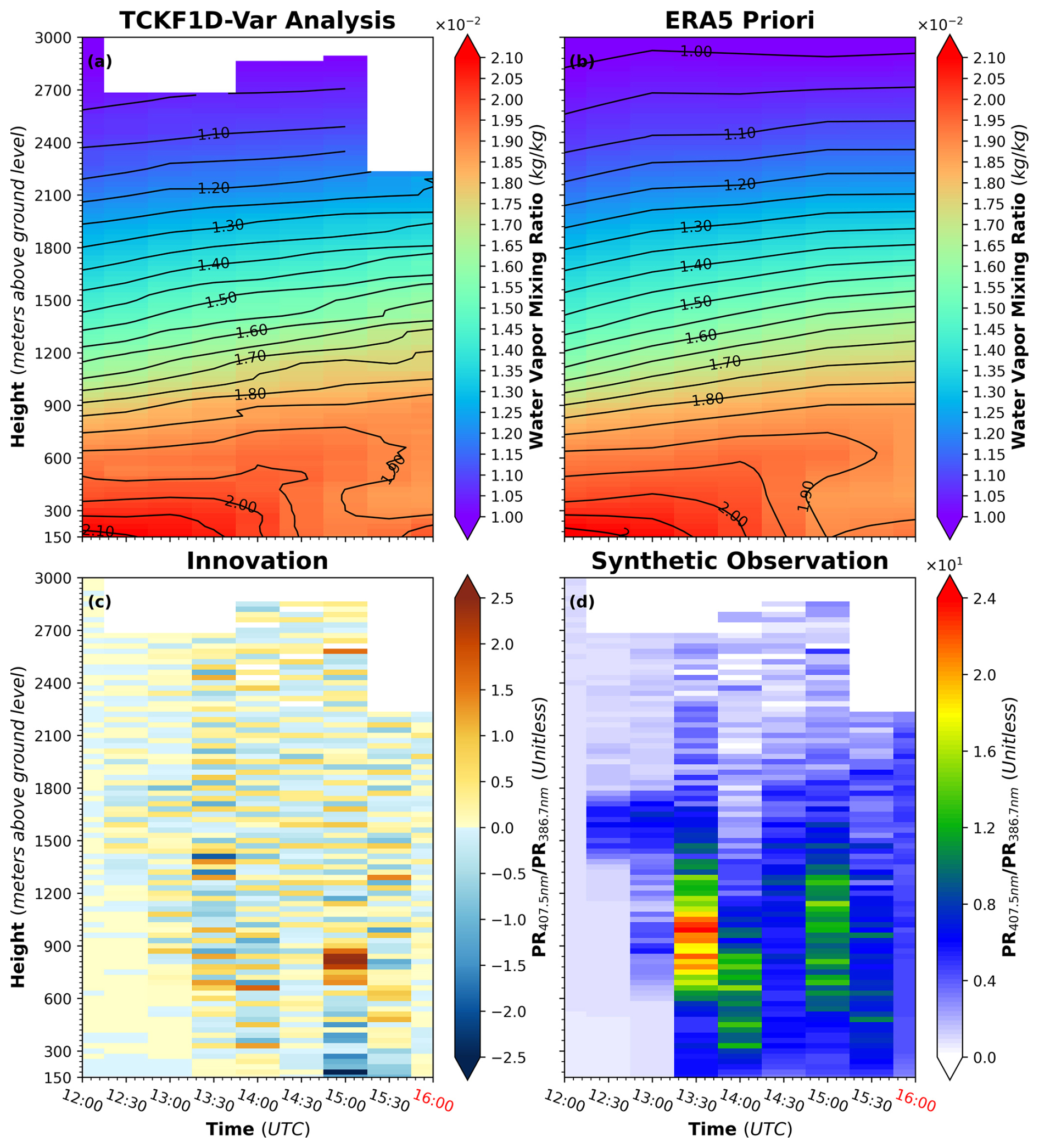
Figure 8 Time–height cross sections of (a) TCKF1D-Var retrieved water vapor mixing ratio at 30 min temporal resolution, (b) ERA5 prior water vapor mixing ratio, (c) Innovation, and (d) synthetic observations derived from the MRL Raman channel measurements, for the nighttime heavy precipitation case with maximum hourly rainfall intensity at station 59293 (16:00 UTC on 31 July 2025). The red-colored x-axis tick label (16:00 UTC) denotes the precipitation occurrence time.

The minimum hourly rainfall case (Fig. 9) occurred at station 54218 at 19:00 UTC on 26 July 2025, with an hourly accumulated precipitation amount of 10.7 mm. Although identifiable analysis increments are also evident in this case, their vertical distribution differs markedly from that of the maximum rainfall event. The analysis increments are mainly concentrated above 1200 m and are most pronounced within the 2100–3000 m layer, consistent with the statistical characteristics identified in Sect. 3.2 (Fig. 6a). Similar to the maximum rainfall case, the Innovation field exhibits temporal–vertical structures consistent with those shown in Fig. 9a and b. Meanwhile, the reconstructed observations (Fig. 9d) display progressively increasing magnitude and vertical variability as precipitation onset approaches. These results demonstrate that the TCKF1D-Var framework, together with the MRL Raman channel observations, is capable of capturing coherent moisture structure variations prior to precipitation under different rainfall intensity conditions.

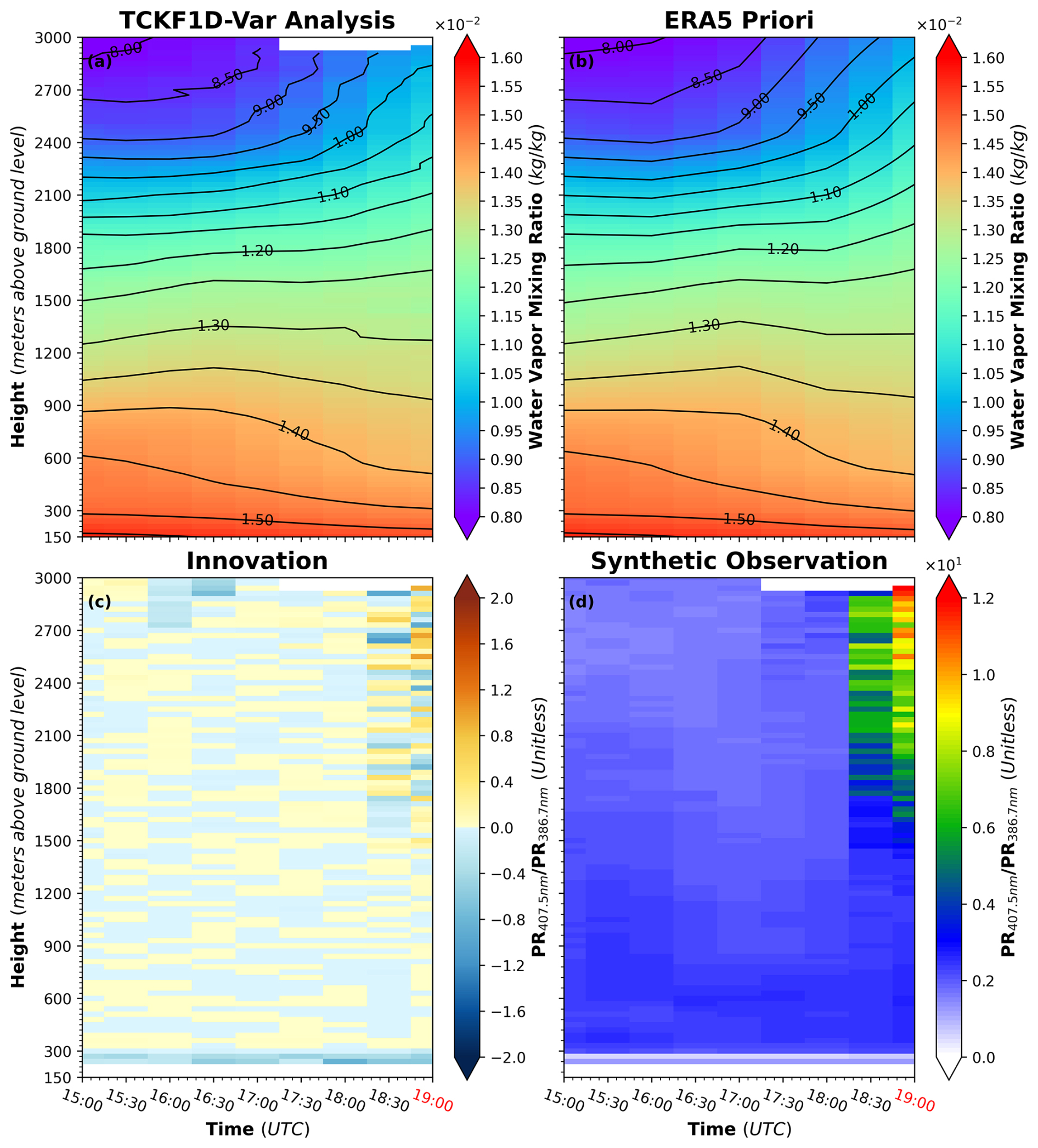
Figure 9 Time–height cross sections of (a) TCKF1D-Var retrieved water vapor mixing ratio at 30 min temporal resolution, (b) ERA5 prior water vapor mixing ratio, (c) Innovation, and (d) synthetic observations derived from the MRL Raman channel measurements, for the nighttime heavy precipitation case with minimum hourly rainfall intensity at station 54218 (19:00 UTC on 26 July 2025). The red-colored x-axis tick label (19:00 UTC) denotes the precipitation occurrence time.

The median-like hourly rainfall case (Fig. 10) occurred at station 56492 at 16:00 UTC on 10 August 2025, with an hourly accumulated precipitation amount of 26.9 mm, which is closest to the median precipitation amount of 25.1 mm listed in Table 3. Comparison between the TCKF1D-Var retrieved profiles and the ERA5 prior profiles (Fig. 10a and b) again reveals clear analysis increments, indicating substantial adjustments relative to the ERA5 prior state. However, the temporal and vertical characteristics of these increments differ from those identified in Figs. 8 and 9. Within the 1200–3000 m layer, clear departures from ERA5 become evident approximately 2 h before precipitation onset, which is shorter than the lead time identified in the minimum rainfall case, where similar differences emerged nearly 3 h prior to precipitation. In addition, the magnitude of the analysis increments within the 1200–3000 m layer is weaker than that observed in the minimum rainfall case. Below 1200 m, the TCKF1D-Var retrieved profiles also begin to deviate from ERA5 approximately 2 h before precipitation onset, consistent with the timing identified in the maximum rainfall case. Nevertheless, the main region of enhanced analysis increments is confined to the 600–1200 m layer, which is narrower than the corresponding layer identified in the maximum rainfall case (150–1200 m). The magnitude of the low-level analysis increments is also weaker than that in the maximum rainfall event.

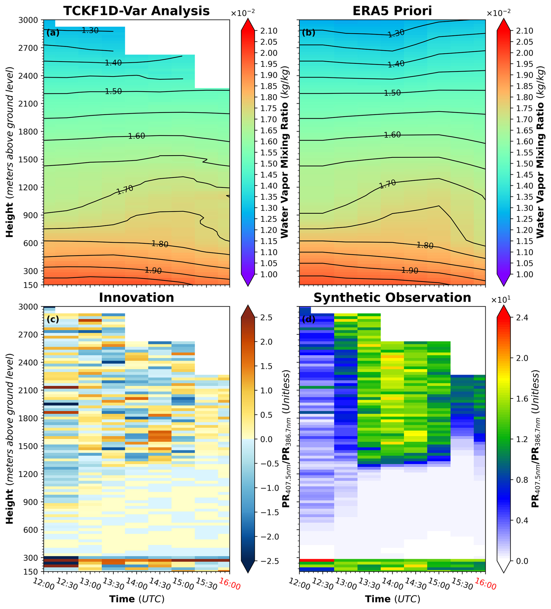
Figure 10 Time–height cross sections of (a) TCKF1D-Var retrieved water vapor mixing ratio at 30 min temporal resolution, (b) ERA5 prior water vapor mixing ratio, (c) Innovation, and (d) synthetic observations derived from the MRL Raman channel measurements, for the nighttime heavy precipitation case with minimum hourly rainfall intensity at station 56492 (16:00 UTC on 10 August 2025). The red-colored x-axis tick label (16:00 UTC) denotes the precipitation occurrence time.

Since all three representative cases exhibit substantial analysis increments relative to the ERA5 prior profiles, and the timing, vertical distribution, and magnitude of these increments appear to vary systematically with precipitation intensity, additional composite analyses were conducted for the three precipitation categories listed in Table 3. Specifically, composite analysis increments of the TCKF1D-Var retrieved water vapor mass mixing ratio profiles were calculated for the 10–20, 20–30, and ≥ 30 mm hourly accumulated precipitation groups to investigate their temporal–vertical evolution prior to precipitation onset (Fig. 11). For the 10–20 mm precipitation category (Fig. 11a), the analysis increments are generally negative below 900 m and positive above 900 m. During the final 90 min before precipitation onset, this vertically stratified structure becomes increasingly pronounced, indicating an enhanced vertical contrast in the moisture analysis increments prior to precipitation initiation. For the 20–30 mm precipitation category (Fig. 11b), positive analysis increments are evident above 450 m during the period from 240 to 180 min before precipitation onset. During the subsequent 180–30 min period, the positive increments within the 1500–3000 m layer gradually transition into negative values, while the increments within the 450–1500 m layer remain positive but with substantially weaker magnitude. In contrast, the 300–450 m layer maintains persistently negative analysis increments throughout the entire pre-precipitation period, consistent with the characteristics identified for the 10–20 mm category. For the ≥ 30 mm precipitation category (Fig. 11c), the analysis increments exhibit a pronounced structural transition approximately 120 min before precipitation onset. During the earlier stage (240–120 min prior to precipitation), the analysis increments are predominantly negative below 1200 m and positive above 1200 m. However, during the final 120 min before precipitation onset, the previously negative low-level increments transition into positive values, and their magnitude increases progressively as precipitation onset approaches. A similar temporal enhancement is also evident within the 1200–3000 m layer, although the increase is substantially stronger than that below 1200 m.

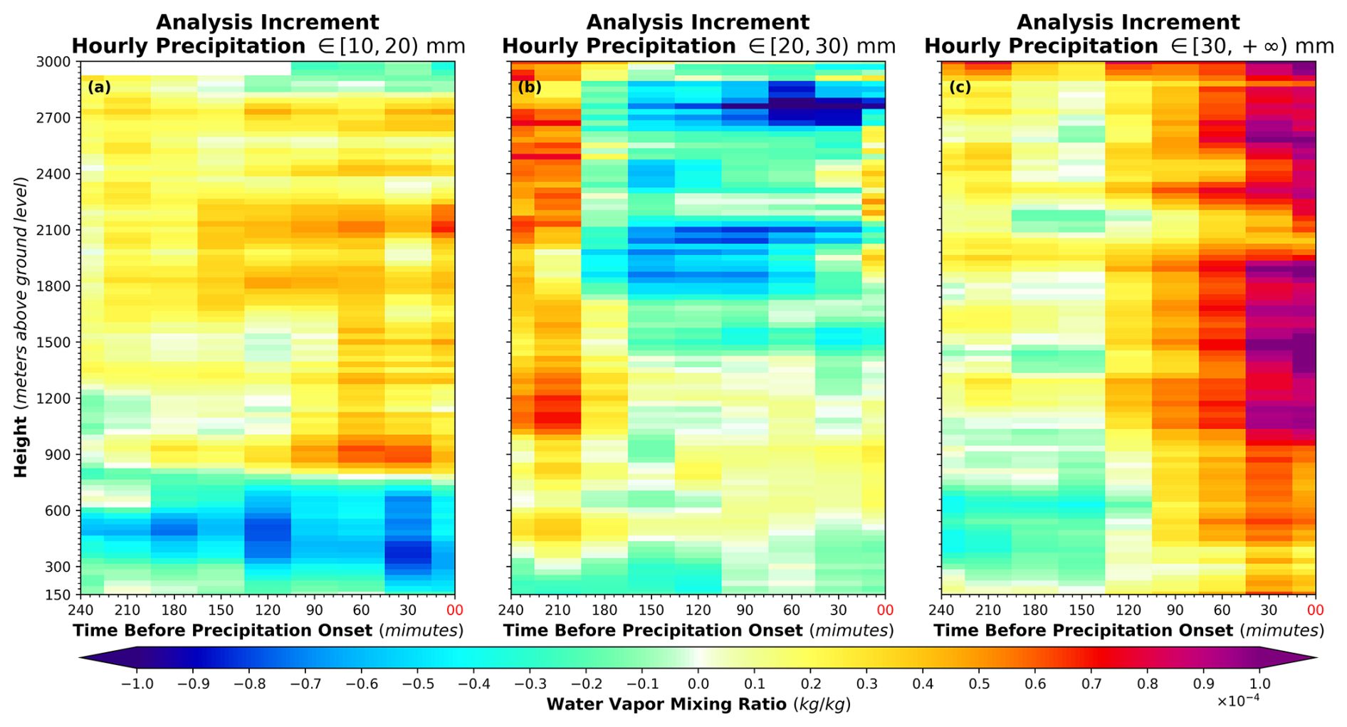
Figure 11 Temporal–vertical evolution of the case-averaged analysis increments in the TCKF1D-Var retrieved water vapor mass mixing ratio profiles relative to the ERA5 prior before the onset of nocturnal heavy precipitation for three hourly accumulated precipitation categories: (a) 10–20 mm, (b) 20–30 mm, and (c) ≥ 30 mm. The red-colored x-axis tick label (00 min) denotes the precipitation occurrence time.

Overall, these results demonstrate that the TCKF1D-Var retrieved water vapor mass mixing ratio profiles not only provide substantial adjustments relative to the ERA5 prior profiles, but also exhibit temporally and vertically coherent analysis increment structures prior to nocturnal heavy precipitation. More importantly, the evolution characteristics of these analysis increments appear to be systematically associated with precipitation intensity, as represented by the hourly accumulated precipitation amount.

4 Summary and concluding remarks

In this study, we extend a previously developed and validated thermodynamic- and cloud-microphysics-constrained Kalman filter one-dimensional variational (TCKF1D-Var) framework to incorporate nitrogen and water vapor Raman channel observations from the Mie–Raman lidar (MRL) network of the China Meteorological Administration. A physics-informed lidar observation operator was developed based on the classical Raman lidar formulation. To account for time-varying instrumental performance and aerosol-related uncertainties, a data-driven calibration component was introduced as a multiplicative correction while preserving the underlying physical structure of the forward model. In addition, a Kalman filter-based observation fusion approach with dynamically estimated process and observation error covariance matrices was implemented to improve retrieval robustness under low signal-to-noise conditions.

The performance of the proposed method was evaluated against co-located radiosonde observations launched prior to nocturnal heavy precipitation events at 56 stations across China in 2025. The results demonstrate that the TCKF1D-Var retrievals, with a vertical resolution of 30 m and a temporal resolution of 30 min, consistently reduce both mean bias and root mean square error relative to the ERA5 prior profiles. The improvement is relatively pronounced within the 1.2–3.0 km layer above ground level. Sensitivity experiments further indicate that the selected 30 min temporal window provides a favorable balance between observational information and forward-model uncertainty for the MRL observations.

Application to nocturnal heavy precipitation events shows that the retrieved water vapor mass mixing ratio profiles capture coherent temporal–vertical variations in boundary-layer moisture prior to precipitation onset. In particular, a persistent moistening signal relative to the ERA5 prior is identified within the 1.2–3.0 km layer, with increasing magnitude as the precipitation onset approaches. These results suggest that the integration of MRL Raman channel observations within a physically constrained retrieval framework can provide valuable information on pre-convective moisture evolution.

Despite the encouraging results, several limitations should be noted. First, the data-driven calibration component is designed to represent effective corrections to the observation operator, but it does not explicitly separate instrumental, aerosol, and model-related error sources. Second, the estimation of process and observation error covariance matrices relies on statistical approximations within a finite temporal window and may not fully capture all sources of uncertainty. Third, the retrieval performance is primarily evaluated against radiosonde observations; further assessment using additional independent datasets is needed to better characterize retrieval uncertainties under a wider range of atmospheric conditions. In addition, the choice of temporal resolution involves a trade-off between noise reduction and the ability to resolve rapid atmospheric variability, which may vary under different meteorological conditions.

Although the present study demonstrates consistent improvements over the ERA5 prior profiles, the overall accuracy gain is still relatively modest (approximately 5 %), indicating that considerable room for improvement remains before the retrievals can fully meet the requirements of high-impact applications. In the next stage, our efforts will concentrate on improving the physical representation of the lidar observation operator, particularly through the development of a more explainable data-driven calibration approach to better characterize time-varying instrumental and aerosol-related effects. In parallel, the estimation of the process and observation error covariance matrices will be further refined to provide a more realistic representation of observation and model uncertainties associated with boundary-layer turbulence. Additional observational constraints will also be incorporated, including temperature-sensitive measurements from rotational Raman channels of Raman lidars with atmospheric temperature profiling capability, which are expected to further enhance the accuracy and robustness of the retrieved water vapor mass mixing ratio profiles. Once the retrieval accuracy has been further improved, future studies will investigate their application in data assimilation–numerical weather prediction systems to assess their potential contribution to representing pre-convective moisture conditions in short-term forecasts and severe weather early warning. Such investigations, however, require dedicated assimilation experiments and are beyond the scope of the present study.

Appendix A: Kalman Filter–Derived P and R Matrices

Figure A1 presents the R matrices diagnosed during the water vapor profile retrieval process using all precipitation cases listed in Table 3. The results reveal substantial differences in the structure of the diagnosed R matrices across precipitation intensity categories, indicating that the characteristics of observation errors vary with the rainfall environment. For cases associated with hourly accumulated precipitation between 10 and 20 mm (Fig. A1a), a pronounced vertical correlation is evident, with the strongest correlated region extending approximately from 900 to 1600 m above ground level. In contrast, the cases with hourly precipitation between 20 and 30 mm (Fig. A1b) exhibit relatively weak vertical correlations, and no distinct coherent correlation structure can be identified. For the most intense precipitation cases, characterized by hourly accumulations exceeding 30 mm (Fig. A1c), the enhanced vertical correlations are primarily confined to the lower atmosphere, with the largest values concentrated between 150 and 600 m.

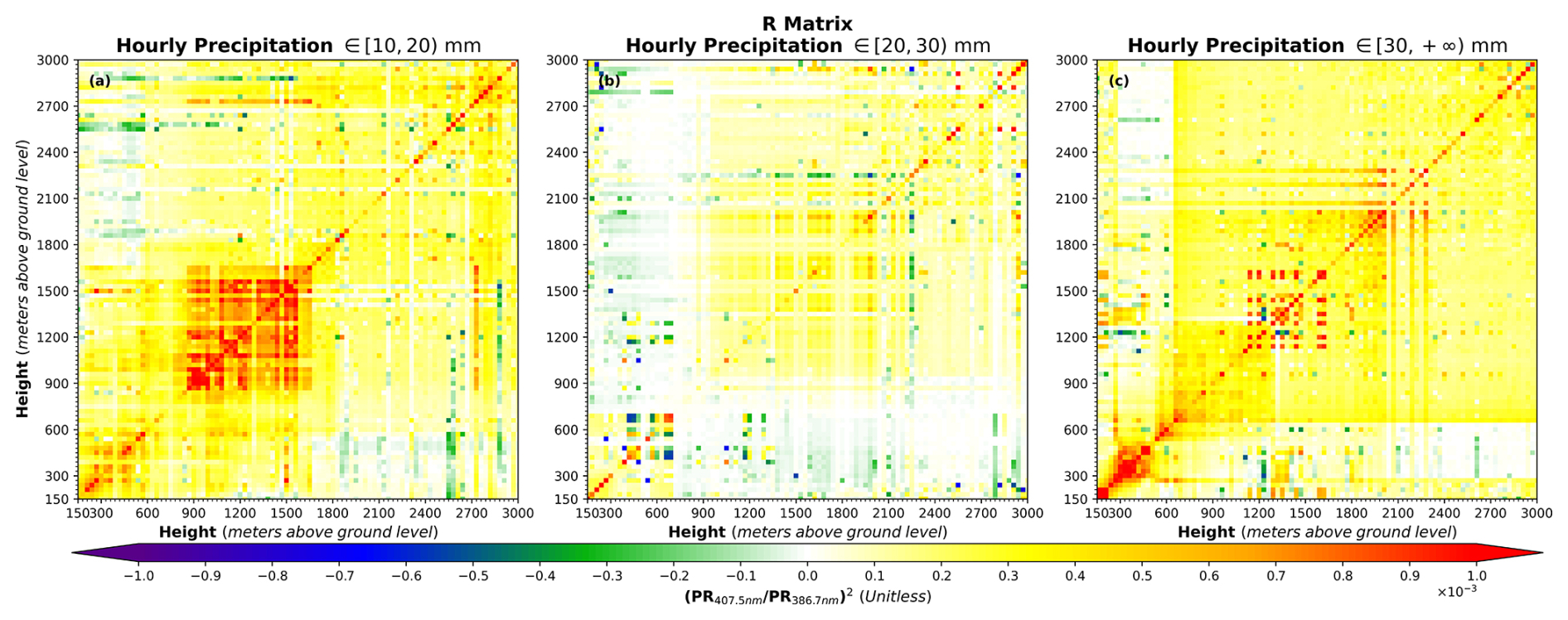
Figure A1 R matrices for water vapor profile retrievals derived from all precipitation cases listed in Table 3. Panels (a), (b), and (c) correspond to cases with hourly accumulated precipitation of 10–20, 20–30, and > 30 mm, respectively.

Figure A2 presents the P matrices diagnosed during the water vapor profile retrieval process for all precipitation cases listed in Table 3. Compared with the R matrices shown in Fig. A1, the diagnosed P matrices display much weaker vertical correlations, with no pronounced coherent correlation structures evident in any of the precipitation categories. Furthermore, the overall covariance patterns are largely consistent among cases with hourly accumulated precipitation of 10–20 mm (Fig. A2a), 20–30 mm (Fig. A2b), and greater than 30 mm (Fig. A2c).

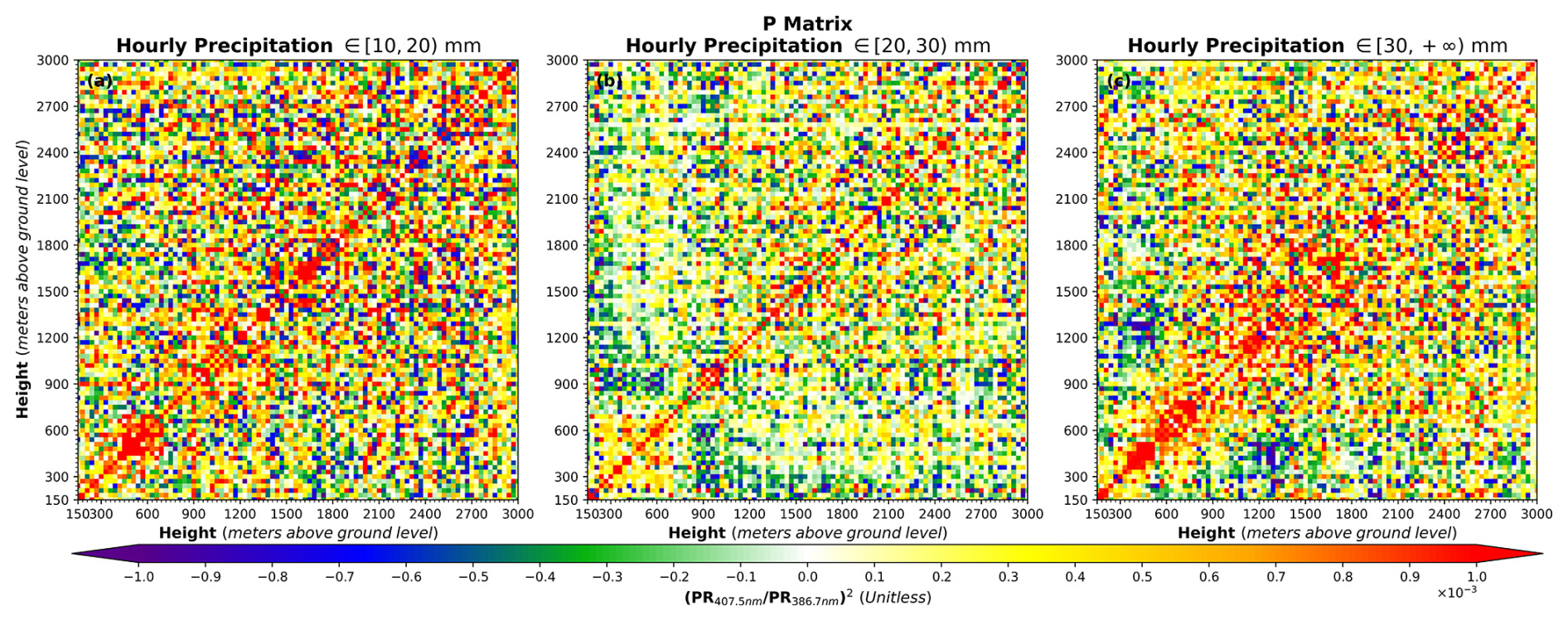
Figure A2 P matrices diagnosed during the water vapor profile retrieval process for all precipitation cases listed in Table 3. Panels (a), (b), and (c) correspond to cases with hourly accumulated precipitation of 10–20, 20–30, and > 30 mm, respectively.