A machine learning method for estimating atmospheric trace gas concentration baselines

Estimates of trace gas baseline mole fractions in high-frequency atmospheric measurement records are crucial for analysing long-term changes in atmospheric composition. Baseline mole fractions are those that would be observed far from emission sources (and hence are representative of background conditions). Previous methods for inferring baseline mole fractions have used statistical or meteorological approaches, or, if available, co-measured tracer species thought only to be emitted from non-baseline wind sectors. Combinations of these techniques have also been employed in some applications. Statistical methods typically fit a baseline to the observations themselves, while meteorological methods use atmospheric models of varying complexity to categorise air mass origins. In this paper, we present a novel machine learning method for estimating trace gas baseline mole fractions, which benefits from the physical basis of model-based filtering without the need for running an expensive simulator. Our approach offers the accessibility and computational cost-effectiveness of statistical models, without the associated smoothing or difficulty in identifying rapid baseline variations. By training on historical Lagrangian particle dispersion model outputs, our model learns to predict baseline mole fractions directly from meteorological fields. This advancement opens new avenues for low-latency trace gas time series data analysis, reconstruction of historical baseline trends, and improved utilisation of tracer measurement air mass classification methods.

1 Introduction

The evaluation of long-term trends in the concentration of atmospheric trace species is important for understanding phenomena such as stratospheric ozone depletion and climate change. However, a challenge associated with the analysis of high-frequency (∼ hourly to daily) trace gas measurements is the separation of “baseline” concentrations from measurements strongly influenced by nearby sources. Here, we define baseline measurements as concentrations that would be observed at a point in the atmosphere, if it were not influenced by nearby sources or sinks (e.g. Manning et al., 2011). Such baseline time series have become essential for understanding hemispheric or global trends in greenhouse gases (for example, the “Keeling curve” for carbon dioxide; Keeling et al., 2005), and ozone depleting substances (e.g. Laube et al., 2022; Liang et al., 2022).

Whether the trace gas mole fraction in a particular air mass is characteristic of the regional baseline or non-baseline conditions depends on the interplay of meteorology and fluxes. Advection from regional sources or sinks to a measurement site over timescales of days to weeks will lead to mole fractions that are above or below the baseline. Enhancements above baseline can also be observed under low wind speeds or planetary boundary layer heights (PBLH), when the measurements are particularly sensitive to local fluxes. Even when the influence of regional fluxes on a particular air mass is small, variations in mole fractions are observed due to long-range transport from latitudes or altitudes with very different baseline mole fractions to that of the measurement site (e.g. Arnold et al., 2018; Lunt et al., 2016).

Measurement networks such as the Advanced Global Atmospheric Gases Experiment (AGAGE) collect mole fraction data for numerous greenhouse gases (GHGs) and ozone-depleting substances (ODSs) at several locations around the world at approximately hourly frequency (Prinn et al., 2018). These monitoring stations observe baseline concentrations, overlaid with time-varying enhancements or depletion events for the reasons outlined above. Data filtering is therefore needed to estimate baselines, or categorise the data points that best reflect baseline concentrations.

As an example, Fig. 1 shows AGAGE measurements of the hydrofluorocarbon HFC-134a (C₂H₂F₄), at Mace Head, Ireland, and Gosan, Republic of Korea. Widespread use of this compound as a refrigerant has resulted in increasing global atmospheric abundances (Liang et al., 2022). The measurements at Mace Head, Ireland, are characterised as baseline when air originates from the Atlantic to the west, but these can be overlaid with enhancements as a result, primarily, of the advection of “polluted” air masses from European sources to the east (raw data are shown as grey lines in Fig. 1, with overlaid coloured crosses indicating baseline/non-baseline). At Gosan, enhancements are seen when air originates from a wider range of wind directions, due to surrounding sources from China to the west, the Korean peninsula to the north and Japan to the east. Furthermore, during the summer months, intrusions of Southern-Hemispheric air are frequently seen, associated with the observation of below-Northern-Hemispheric mole fractions. The investigator may or may not wish to include baseline mole fractions originating from latitudes that are very different to the measurement station, depending on the application. For example, when estimating the long-term mole fraction trend using observations from Mace Head, Ireland, air masses originating from the tropical Atlantic were removed in Manning et al. (2021), but a summertime baseline more characteristic of the Southern Hemisphere was included in the inverse modelling study using Gosan data in Arnold et al. (2018).

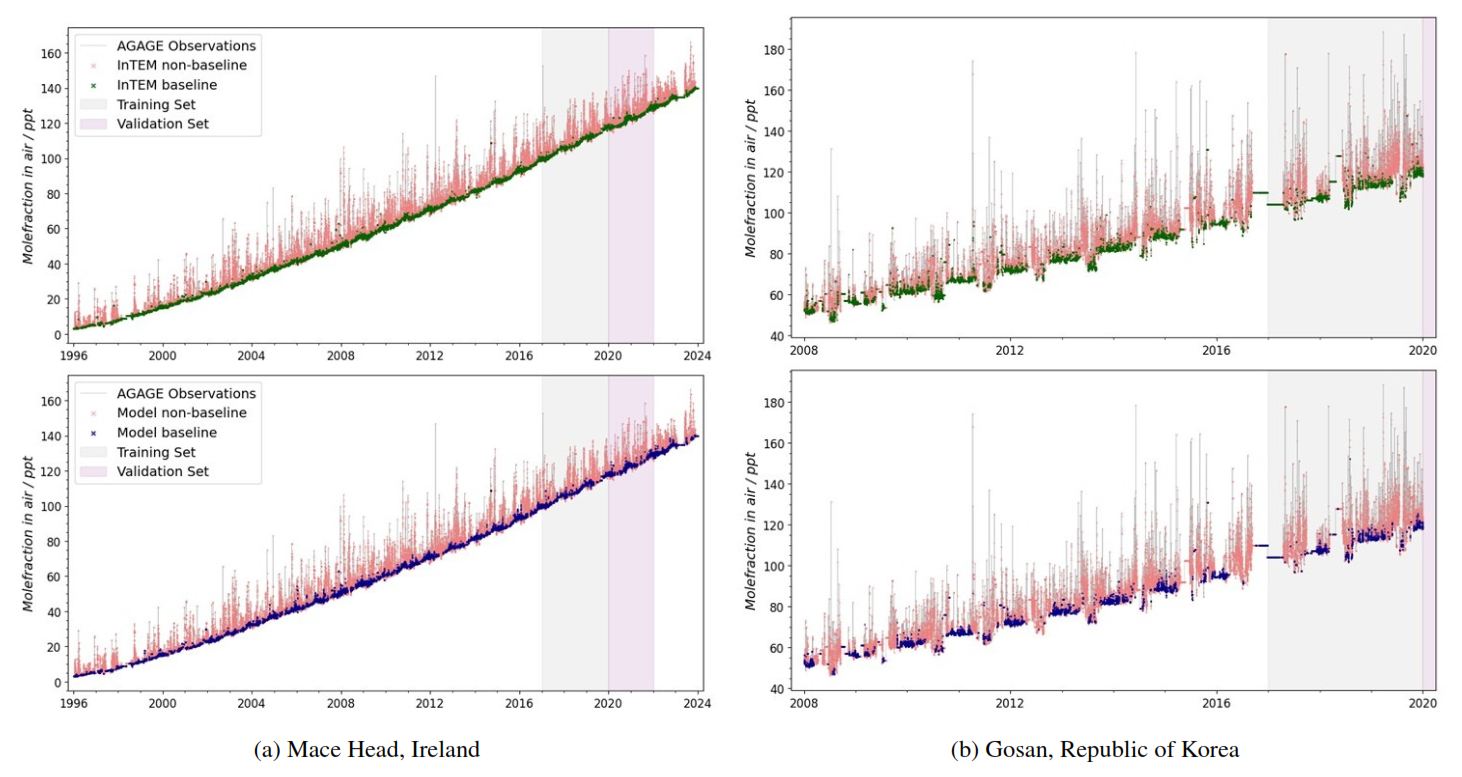
Figure 1 Measurement time series for HFC-134a (CH₂FCF₃) at (a) Mace Head, Ireland, and (b) Gosan, Republic of Korea. The observations are shown as crosses and coloured according to the baseline/non-baseline label. The top panels show the measurements identified as baseline using the NAME/InTEM footprint-based filtering approach with no statistical filtering applied (green), and the bottom panels show the data points classified by the MLP algorithm presented here to be baselines (blue). The three-year training period is shown as grey shading and the two validation years are indicated by purple shading.

Previous baseline classification or fitting algorithms have broadly used three types of approach: statistical filtering, meteorological filtering or filtering based on co-measurement of some tracer for non-baseline conditions. Measurement-based methods have used species such as ²²²Rn or carbon monoxide (CO) to identify air masses substantially influenced by terrestrial sources or anthropogenic activity, respectively (e.g. Chambers et al., 2016, 2013; Yang et al., 2009). Since they require deployment of additional specialist instrumentation, we will not discuss them further here, although we note that our proposed approach could use measurements of these tracers as a training dataset.

Baseline identification through pure statistical filtering is seen in many studies, with examples including the use of iterative polynomial fitting with exclusion of outliers, and filtering of certain frequencies using Fourier transforms (O'Doherty et al., 2001; Ruckstuhl et al., 2012; Thoning et al., 1989; Novelli et al., 1998). O'Doherty et al. (2001) outlines the AGAGE baseline algorithm, which iteratively fits a polynomial to the measurement time series and excludes points that are more than 3 standard deviations above the median within some time window (121 d). Similarly, Novelli et al. (1998) used a polynomial fit, including harmonic terms, with a low-pass filter to exclude above-baseline measurements. Their approach was subsequently improved to transform the residuals to and from the frequency domain and apply high and low-pass filters in Novelli et al. (2003). Ruckstuhl et al. (2012) describe the “Robust Estimation of Baselines (REBS)” approach, which uses local regression within some defined time window to estimate the baseline and the distribution of its observed values. Each of these statistical methods has the advantage of requiring no ancillary data or model simulations to apply, and is computationally efficient. However, due to the use of polynomial fitting or moving windows over which data are excluded or regression is performed, they all implicitly or explicitly apply some smoothing to the data, which may not be characteristic of the true baseline variability. Furthermore, they cannot readily identify or remove baseline values that are characteristic of a latitude different from that of the measurement station (as observed, for example, when southerly air masses arrive at Mace Head or Gosan; Fig. 1).

Meteorological filtering techniques have often used air mass back trajectories (estimates of advective transport prior to an observation), or wind sector analysis, to identify air masses that are unlikely to be strongly influenced by regional fluxes. Henne et al. (2008), Lööv et al. (2008), and Salvador et al. (2010) computed back trajectories, and then applied a clustering algorithm to explore patterns in air mass origins. Alternatively, several studies (Derwent et al., 1998a, b; O'Doherty et al., 2001) have applied a wind sector allocation approach, described in detail by Derwent et al. (1998c) to isolate air masses originating from some wind sector thought not to be strongly influenced by local fluxes.

In an extension of back-trajectory-based methods, recent studies have used trace gas source-receptor relationships (“footprints”), calculated using Lagrangian particle dispersion models (LPDMs), to estimate the full influence of transport and mixing on observed concentrations. A range of particle dispersion models have been applied to baseline estimation, including the UK Met Office Numerical Atmospheric Modelling Environment (NAME) (Ryall et al., 1998; Manning et al., 2011), which we use in this study. LPDMs estimate footprints by considering the transport of an ensemble of hypothetical gas particles backwards in time, driven by archived meteorological fields. For the NAME simulations used in this study, these are obtained from the UK Met Office Unified Model analyses (Cullen, 1993). LPDM footprints quantify the contribution to the observed concentration of a unit emission from the surface at each grid cell surrounding the measurement point (Manning et al., 2011).

Manning et al. (2021) combined LPDM footprints with a population density map to identify air masses that were potentially influenced by anthropogenic emissions (illustrated in Fig. 2). A flux proportional to population density was transported through the NAME model atmosphere to produce a synthetic anthropogenic tracer at each measurement site. When the concentration of this tracer fell below some arbitrary threshold, the corresponding air mass was labelled as being representative of the baseline. This method, part of the Inversion Technique for Emission Modelling (InTEM) (Manning et al., 2011), has been applied in a number of studies (Arnold et al., 2018; Lunt et al., 2021). In addition to baseline classification, the method also categorises air masses further into a set of classes specific to a given site. For Mace Head, Ireland, for example, air masses are either “southerly” (when air masses originate from lower latitudes, specific for European sites), “local” (where local influences may dominate due to low ventilation conditions), “polluted” (where potential anthropogenic influence is high), “mixed” (when there is a combination of source types), “upper troposphere” (when air masses have descended from higher altitudes), or baseline. Figure 2 shows two example footprints for Mace Head, Ireland, superimposed on a population density plot to illustrate the approach. Figure 2a shows conditions consistent with baseline mole fractions for compounds whose fluxes are highest over land; the footprint is primarily over the ocean and does not deviate substantially in latitude from the measurement location. Figure 2b shows an instance where the air mass originates from more populated and industrialised regions, where enhanced concentrations are typically observed.

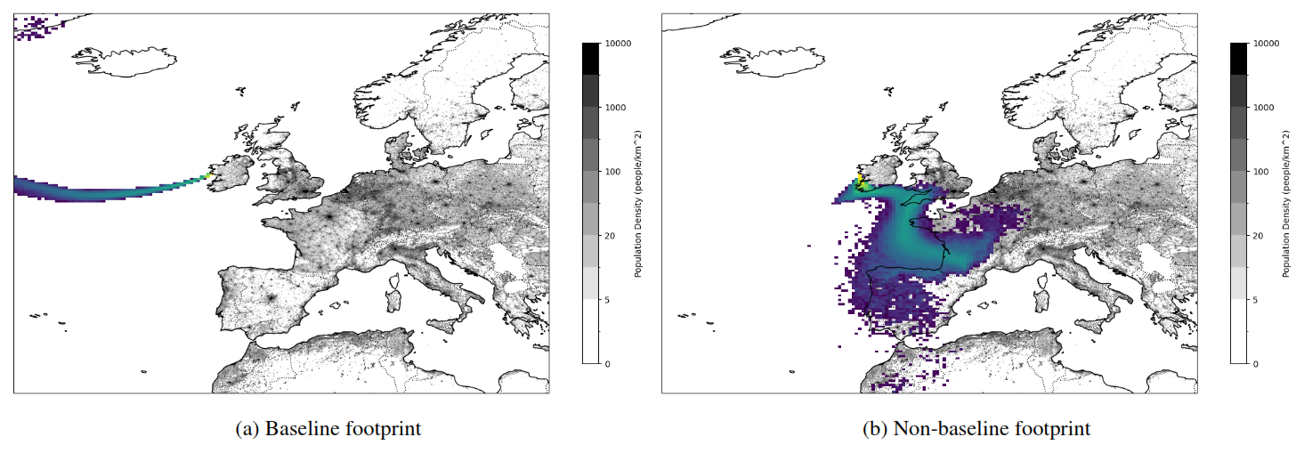
Figure 2 Two example NAME footprints showing incoming air masses to Mace Head atmospheric research station that illustrate meteorology consistent with, (a) baseline and (b) non-baseline observations. The footprint colour refers to the susceptibility of the measurement to emissions from that grid cell on a logarithmic scale; green represents higher values, and purple, lower (colourbar not shown). Population density is also shown as a proxy for anthropogenic flux magnitude (grey shading).

Unlike statistical filters, model-based baseline classifications do not impose smoothing on the dataset and airmass categories can be justified based on a more complete range of physical considerations than simple meteorological filtering (e.g. based on small numbers of trajectories or wind sectors). Therefore, this approach is generally considered the gold standard for baseline classification, when co-emitted tracer measurements are not available. However, such methods are computationally costly and technically challenging to implement. Here, we present a baseline classification algorithm using a machine learning (ML) approach that emulates an LPDM-based filter. Our approach preserves the benefits of a meteorological filter for a fraction of the computational cost.

ML has been employed successfully for various applications in atmospheric chemistry, including the prediction of particulate matter concentrations and nitrogen dioxide modelling (Brokamp et al., 2018; Masih, 2019). Also, ML-based LPDM footprint emulation is an increasingly active area of research; recent methodologies such as Fillola et al. (2023), FootNet (He et al., 2025) and GATES (Fillola et al., 2026) demonstrate the potential of ML-based surrogates in this field. Whilst this study focuses on baseline identification rather than full footprint reconstruction, these approaches show the broader capabilities of ML-based frameworks for emulating LPDM-based diagnostics.

The aim of this study is to investigate the application of ML for the classification of trace gas baseline air masses, in order to accurately recreate the air mass categories obtained from the Met Office NAME/InTEM LPDM-based algorithms. The method identifies data points likely representing background conditions, separating them from those with substantial local emission contributions. It does not attempt a quantitative decomposition of individual observations into separate background and local source components. We demonstrate this method at nine different AGAGE sites, in a range of meteorological regimes and for a range of compounds. The baseline classification is based only on meteorological inputs, namely wind speed and direction, boundary layer height and surface pressure.

2 Methodology

2.1 Data

2.1.1 Baseline Flags

For the purpose of training our ML algorithm, a dataset of flags that categorise air masses as “baseline” or “non-baseline” using some independent method is required. Here, we use air mass labels, based on outputs from NAME/InTEM (Manning et al., 2021; Jones et al., 2007). The method categorises air masses bi-hourly, with categories tailored for each site (e.g. “baseline”, “polluted”, “local”, “mixed”, “southerly”, “upper troposphere”, for Mace Head). For this work, the categories were simplified to a binary “baseline” vs. “non-baseline” label (grouped non-baseline categories). This restriction was applied to focus on the robust identification of baseline data points for long-term atmospheric composition trend analysis or regional inverse modelling. In the InTEM framework, an additional statistical filter is applied to the derived baseline on a species-by-species basis, to remove any remaining outliers, but the flags used in this study are based only on the footprint-based filter. The algorithm presented here could be retrained with or without the air mass origin conditions described above (e.g. the exclusion of air masses from latitudes different from the measurement site and the Gosan exception), by modifying the training dataset.

2.1.2 Meteorological Data

Meteorological data were obtained from the European Centre for Medium-Range Weather Forecasting (ECMWF) ERA5 reanalysis dataset (Hersbach et al., 2020). These data were downloaded at hourly intervals on a longitude/latitude horizontal grid and hybrid coordinates in the vertical and used as an input to the ML algorithm. The ECMWF meteorological fields were used, rather than the Met Office UM fields that were used to drive NAME, as they were more readily available for longer time periods. An intercomparison of the two products showed close agreement at the AGAGE measurement stations, as would be expected since both products assimilate similar meteorological observations. For example, calculated mean absolute percentage errors gave a less than 10 % error in wind direction across a six-month sample period (January–June 2015) at Mace Head, Ireland. However, wind speed saw a slightly higher error (15.3 %) with UM speeds generally surpassing that of the ERA-5 met products (see Sect. S1 in the Supplement).

2.1.3 Mole Fraction Observations

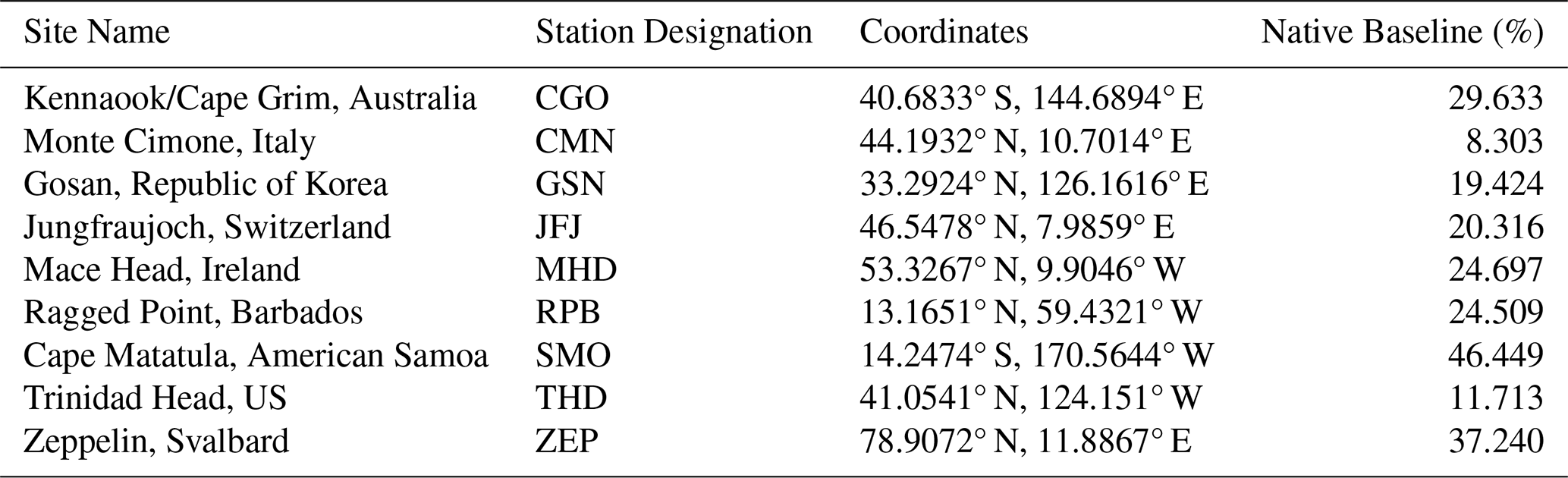
Trace species mole fraction data were obtained from AGAGE (Prinn et al., 2025) at approximately two hour intervals. Measurements are provided as dry air mole fractions (in ppt, equivalent to pmol mol⁻¹ or ppb, nmol mol⁻¹). We demonstrate our algorithm at nine AGAGE sites, covering four continents and spanning a range of remote and relatively “polluted” environments. Details of the chosen sites are outlined in Table 1. All sites have at least 10 years of data, with most having more than 20. This is equivalent to over 200 000 measurements across the nine sites.

Table 1 Details of selected AGAGE sites, with site designation and coordinates given. The percentage of native baseline flags across the full investigation period (training, validation and testing) is also given.

2.2 Preprocessing

The mole fraction and meteorological datasets were combined by aligning them to the InTEM baseline flag time period.

Initial exploration of the datasets showed a significant imbalance between the baseline and non-baseline classes, with seven of the nine sites seeing baseline points being less than one-third of the dataset. The effect of class balance on model performance was explored by varying the percentage of baseline points in the training set (by randomly under-sampling the non-baseline class), and by implementing a sample weight system that assigns more importance to the baseline observations, accounting for the natural class imbalance without needing to remove any training data points. The optimal baseline proportion and sample weighting was found to be both model- and site- specific, although the proportion of baselines was always within 20 %–40 % and the sample weight did not exceed 3. The exact values can be found in the Supplement (Sect. S4.2).

2.3 Model Inputs

The meteorological parameters included as inputs or features to the ML model were the eastward and northward wind components (m s⁻¹) at 10 $\mathrm{m}\mathrm{a}.\mathrm{g}.\mathrm{l}.$ and at two pressure levels, 850 and 500 hPa, surface pressure (Pa), and boundary layer height (m). These data were interpolated to a 17-point grid system around each site, based on two 3×3 grids covering ±5 and ±10° latitude and longitude. To provide the algorithm with further information on changes in atmospheric conditions, all meteorological variables were also provided at time intervals prior to the measurement point. The number and spacing of these intervals were treated as hyperparameters and optimised individually for each model type and site, with intervals up to 72 h prior to the measurement time tested, to allow the model to capture the recent meteorological history for each location. It was found that, in most cases, adding features at 6, 12, 18, and 24 h prior to the measurement time yielded the best performance. Additionally, two temporal variables were added into the dataset to represent the time of day and the day of year. These two variables were integers ranging from 0 to 23 and 1 to 366, respectively. A list of all input variables can be found in the Supplement (Sect. S2).

Normalisation of the meteorological inputs was explored to account for the range of physical quantities with different units and dynamic ranges. Features were scaled separately for each variable category across the 17-point grid (e.g. all eastward wind components at a given height) by their mean and standard deviation. This normalisation was also treated as a hyperparameter, allowing testing with all model types.

2.4 Machine Learning Models

A multilayer perceptron (MLP) was trained to predict baseline classifications for each of the nine AGAGE sites. The method was also tested using two tree-based methods, a random forest and a gradient boosting algorithm, the results of which can be found in the Supplement (Sects. S7 and S8). The three discussed methods were chosen as they outperformed alternatives in early testing, but it is likely that several other suitable architectures also exist.

2.4.1 Model Training

Models were trained individually for each site. Whilst using one universal model applicable to all sites would be desirable for consistency and reduced training time, early tests showed that a more tailored approach is required here. The classification of baselines is driven by population density maps and site-specific rules, as Manning et al. (2011) does with Mace Head, Ireland, and the transport patterns influencing each site will be strongly driven by the geographical features surrounding that site. Generalisation across sites would require training a more complex model with a substantially larger feature set. The approach taken here, of training a model for each site, means that the geographical characteristics of each location are learned implicitly.

Three years of data were used for model training (approximately 3000 data points); 2017–2019 were arbitrarily chosen. The two years following the training years was used for the validation set (2020 and 2021), and the rest of the dataset was used for testing. Given the substantial auto-correlation on the training dataset, characteristic of synoptic variability, it was important that the training and testing dataset be separated in time by greater than synoptic timescales (∼5–10 d). Three years were chosen for training following an investigation into the balance between length of the training period, model performance, and training time. Improvements seen in model performance when further increasing the volume of training data were too minor to justify the consequent increase in computational demands, as shown in the Supplement (Sect. S3). Two years were chosen for validation as one year was found to not be representative enough to generate reliable metrics at sites with a low native baseline ratio (see Table 1); this validation time period was then applied across all sites for consistency. Using the remaining data for testing allowed the models to be evaluated over long periods, testing their ability to account for a wide range of meteorological conditions.

Model hyperparameters were optimised using grid searches. These grid searches were performed independently for each site, but similar parameter choices were seen in the trained models throughout. For example, all MLP models used the ReLU (rectified linear unit) activation function, which outputs zero for all negative input values but leaves positive ones unchanged to introduce non-linearity to the dataset (Eckle and Schmidt-Hieber, 2019). All sites saw models with three layers in their optimised MLP, with the number of hidden layers and the number of neurons they contain varying. The Mace Head model, for example, consists of an input layer with 682 neurons (all input features plus additional meteorological inputs at 6, 12, 18, and 24 h prior to the measurement time), one hidden layer with 64 neurons, and a single-neuron output layer. Full hyperparameter sets can be found in the Supplement (Sect. S4.1).

A confidence threshold was introduced when making predictions, meaning that the model could only assign a baseline label when the associated confidence exceeded this value (plots showing model-derived baseline confidence are provided in Sect. S9 in the Supplement). This approach was introduced to improve the reliability of the model and reduce the occurrence of false positives. The threshold was treated as a hyperparameter, but optimised as a final step in model training. Again, it was found to be model- and site- specific, and values ranged from 50 % to 70 %.

2.4.2 Model Evaluation

The model was trained to maximise F1 score (Eq. 1), a measure of performance in binary classification problems that averages the precision and recall of a model (Eqs. 2 and 3). Respectively, precision indicates the fraction of all baselines correctly identified as baseline, and recall identifies the fraction of baselines that are correctly identified by the model. The final values that are quoted for these metrics were calculated by considering all data, except for those points used for training and validation. In most cases, the test set exceeded 20 years of data. Note that these metrics define the model's ability to separate baseline and non-baseline samples based only on the air mass meteorology, and so do not consider associated mole fraction values.

$$\begin{array}{}\text{(1)}& {\displaystyle }& {\displaystyle }\text{F1}=\mathrm{2}\times {\displaystyle \frac{(\text{Precision}\times \text{Recall})}{(\text{Precision}+\text{Recall})}}\text{(2)}& {\displaystyle }& {\displaystyle }\text{Precision}={\displaystyle \frac{N\left(\text{true positives}\right)}{N\left(\text{true positives}\right)+N\left(\text{false positives}\right)}}\text{(3)}& {\displaystyle }& {\displaystyle }\text{Recall}={\displaystyle \frac{N\left(\text{true positives}\right)}{N\left(\text{true positives}\right)+N\left(\text{false negatives}\right)}}\end{array}$$

To understand the performance of the ML model in application, the predicted labels can be applied to the atmospheric measurements of a particular compound, and compared to the the NAME/InTEM baseline-only concentration time series. Measurement time series are often aggregated into monthly means in many applications, to remove the influence of short-term fluctuations (Laube et al., 2022; Liang et al., 2022). Therefore, the model was also evaluated by comparing the monthly means derived from the ML emulation to those from the InTEM baseline using three metrics; Mean Absolute Error (MAE), Root Mean Squared Error (RMSE) and Mean Absolute Percentage Error (MAPE). The monthly mean baseline was calculated by collecting and taking the average of all mole fractions labelled as baseline in a calendar month.

To explore the utility of the method across many sites and species, a coefficient of variation (CV) is calculated. This quantifies the noise in the InTEM-derived baseline labels by finding the ratio between the standard deviation and mean across the timeseries, after removing any seasonal variability and the long-term trend. STL decomposition (Seasonal-Trend decomposition based on LOESS) (Cleveland et al., 1990) is applied to the monthly means of the true baseline mole fractions, decomposing each monthly mean m_t into three components:

$$\begin{array}{}\text{(4)}& {\displaystyle }{\displaystyle }{m}_t=T_t+S_t+{\mathit{\epsilon }}_t\end{array}$$

where T_t is the long-term trend, S_t is the seasonal component, and ε_t is the residual. The components T_t and S_t are calculated from the training data (Seabold and Perktold, 2010). As STL decomposition requires a complete time series, any missing months are linearly interpolated prior to decomposition.

For a particular dataset of monthly baseline mole fractions $\mathit{m}=\mathit{\{}{m}_t{\mathit{\}}}_{t=\mathrm{1}}^T$, and residuals $\mathit{\epsilon }=\mathit{\{}{\mathit{\epsilon }}_t{\mathit{\}}}_{t=\mathrm{1}}^T$, the CV is then defined as:

$$\begin{array}{}\text{(5)}& {\displaystyle }{\displaystyle }\text{CV}\left(\mathit{m}\right)={\displaystyle \frac{\mathit{\sigma }\left(\mathit{\epsilon }\right)}{\overline{m}}}\end{array}$$

where σ(ε) is the standard deviation of the residuals and $\overline{m}$ is the mean of m.

2.4.3 Feature importance

We determine the variables that are most important for model performance using a permutation importance analysis (Breiman, 2001; Altmann et al., 2010). Permutation importance is calculated by randomly shuffling the values of a single feature group and observing the resulting change in the model's performance (Fillola et al., 2023). The process is repeated multiple times to ensure robustness, and the importance of a feature is determined by the extent to which model performance degrades when the values of the given feature group are permuted. To account for correlations between individual input features, a known limitation of the permutation importance approach, variables were split into feature blocks prior to analysis (Fillola et al., 2023). Meteorological variables were combined across all times and locations, resulting in five feature groups: the wind u- and v-components, boundary layer height, surface pressure, and temporal features (time of day and day of year). The three most important feature groups for each site are shown in the Supplement (Sect. S6).

3 Results and Discussion

The three model types performed similarly across all nine sites, showing that the limitations of the method lie within the input features rather than the model architecture. For simplicity, in this section we evaluate the MLP model only by considering its ability to correctly identify baseline air masses based on meteorological inputs. We then compare time series for a selection of AGAGE gases. Summary results for all sites are presented, and examples are shown for Mace Head, Ireland, and Gosan, Republic of Korea, chosen because of their very different local emissions, meteorological regimes (e.g. Fig. 1) and native baseline ratios. Results for the random forest and gradient boosting algorithms are presented in the Supplement (Sects. S7 and S8).

3.1 Baseline Identification

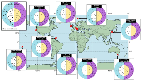
Overall model performance for correctly classifying baseline vs. non-baseline air masses was analysed by considering confusion matrices for each site. These matrices compare the predicted and “true” classifications of the testing set. Figure 3 shows the MLP confusion matrices for the nine AGAGE sites considered in this work. The outcomes of the confusion matrices have been normalised by testing set size and plotted as points on a precision/recall “bullseye” diagram. The inner circles are the MLP model predictions of baseline values. The left half of each diagram represents true baseline points, and the right-hand side are true non-baseline points. Therefore, the correctly identified baselines (true positives) lie in the left-hand segment of the inner circles (white). False positives, or points incorrectly identified as baseline, are in the yellow segment to the right of the inner circle. Points in the blue segment (left-hand side of outer circle) represent missed baselines, or false negatives, whereas the purple area (right-hand side of the outer circle) are true negatives; points identified as non-baseline that are indeed non-baseline. A perfect model would only have points in the white area and the purple area. The fraction of points in the left half of the inner circle (white) compared to the total number in the inner circle (white and yellow) is the precision. The recall is the ratio of points in the inner left circle (white) to the total number of points on the left (white and blue).

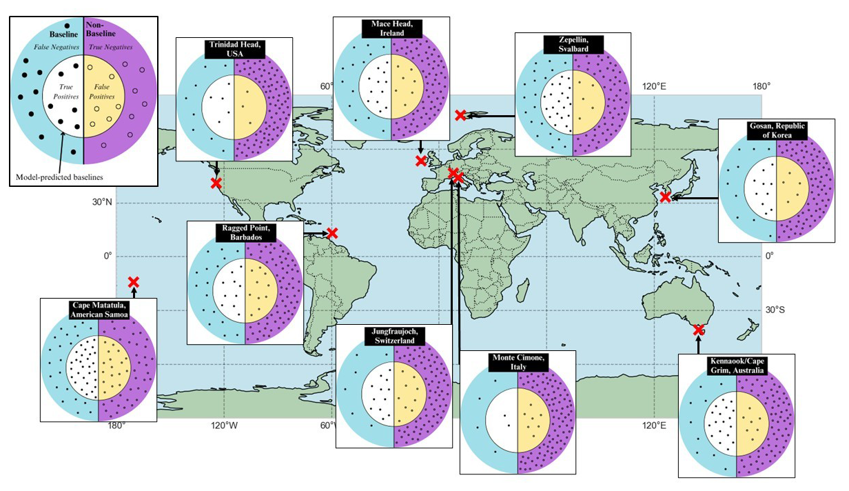
Figure 3 A map showing the locations of the nine AGAGE sites, with confusion matrix-derived plots at each location. Each confusion matrix was normalised, to reduce the visual impact of differences in testing set sizes; each point represents approximately 1 % of the total test set (rounding means that the total number of points on each plot range from 99 to 101). The left half of each circle represents true baseline points, and the right half true non-baseline points. The inner circle shows the MLP model prediction of baseline points. The key in the top left indicates where true or false positives and negatives lie, as explained in the main text.

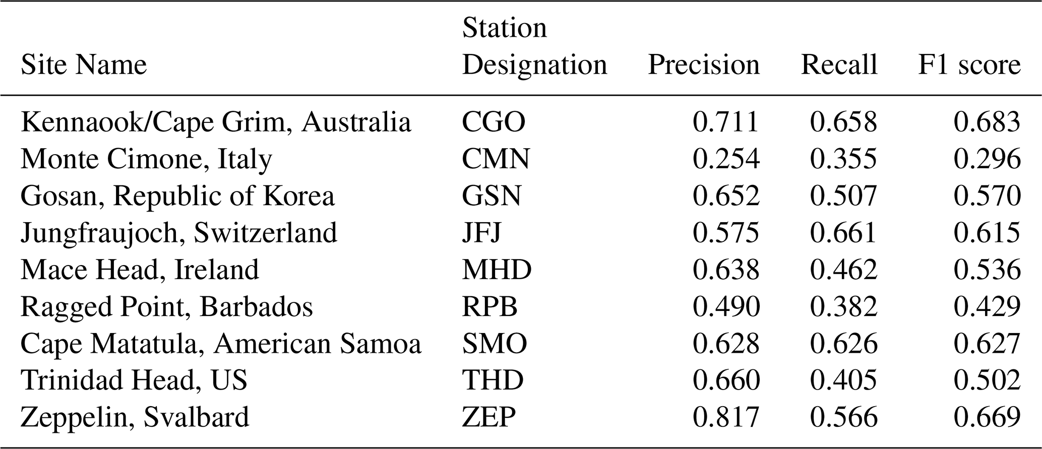
The distribution of points in Fig. 3 reflects optimisation of F1 score in the MLP training, in which a high precision and recall is rewarded jointly; in most cases, the majority of predicted baseline points are true positives (precision) and many of the available baseline points have been correctly identified (recall). These statistics are also summarised in Table 2. As seen in the table, there is some variation between sites, with highest overall scores being obtained at Kennaook/Cape Grim, Australia, and poorer performance at Monte Cimone, Italy, which sees particularly low recall (0.355). These differences are likely a product of both the complexity of the meteorology at the site and the complexity of surrounding fluxes; Kennaook/Cape Grim is a coastal site, whose meteorology is dominated by strongly prevailing westerly flows, whereas Monte Cimone is a mountain site in a region of complex topography. Kennaook/Cape Grim, therefore, sees more baseline meteorological events and so has a higher proportion of baseline data points. Sites with lower baseline proportions (such as Monte Cimone), are more challenging. Our features, which are a subset of meteorological variables on a relatively low-density grid around each site, may not capture well the flows in regions of more inhomogeneous topography and meteorology. Furthermore, in some cases, the outer grid (±10°) may not be enhancing model performance, but may instead add noise, if it is frequently in a different meteorological regime to the measurement site (e.g. in a different meteorological hemisphere, as may sometimes be the case at Ragged Point, Barbados, and Cape Matatula, American Samoa). Restricting the domain to the inner grid (±5°) and/or replacing the outer grid with a smaller, higher-resolution one, may improve model performance at some sites.

Table 2 A tabular summary of the final MLP model outcomes, showing precision, recall and F1 score values for each of the AGAGE sites. Scores can range from 0 to 1, with higher scores indicating higher performance.

Our feature importance analysis (Sect. 2.4.3) reveals that wind components are typically the most critical for model performance, with PBLH and surface pressure generally being of lower importance (see Sect. S6 in the Supplement). However, it should be noted that these variables will be strongly correlated with one-another, so it is not possible to fully isolate the influence of each variable individually. Additionally, in most cases, the analysis showed that the models were not learning much from the two temporal features (time of day and day of year), and so these can likely be removed without negatively impacting model performance. This feature importance pattern aligns with that seen in ML-based LPDM footprint emulation studies (Fillola et al., 2023; He et al., 2025).

3.2 Baseline mole fractions

Whilst the above analysis demonstrates the model's ability to categorise air masses into baseline or non-baseline points, perhaps the most important test of the algorithm is in its ability to reproduce quantities that are used in real-world applications. Here, we focus on the simulation of baseline mole fractions and evaluate the model's ability to calculate robust baseline monthly means, which are commonly used to track changes in greenhouse gases and ozone depleting substances (e.g. Laube et al., 2022; Liang et al., 2022; Gulev et al., 2021).

The model was applied to a subset of 10 atmospheric trace species measured by the AGAGE network (Prinn et al., 2025). These 10 compounds were chosen to span a range of sources, atmospheric lifetimes, and atmospheric histories (e.g. those that are growing in the atmosphere, such as HFCs, vs. those that are declining, such as CFCs).

Examples of the baseline flags applied to HFC-134a measurements at Mace Head and Gosan are shown in Fig. 1. The figure reflects the accuracy of the categorisation shown in Fig. 3; the majority of the InTEM baseline points are identified correctly. The influence of false positives is seen as a number of apparently above-baseline points that are categorised as baseline (noting that a small number of these elevated points are incorrectly flagged as baseline in InTEM, which is why their full algorithm includes a subsequent statistical filtering step). At Gosan, similar to InTEM, the MLP algorithm identifies baseline values in the summer period, which sees Southern Hemispheric air intrusions. The rapid variation between Northern and Southern Hemispheric baselines would be very difficult to detect with statistical filters, which rely on baselines being smoothly varying. Similar plots for all other sites and the chosen sample species (those defined in Table 3) are shown in the Supplement (Sect. S9).

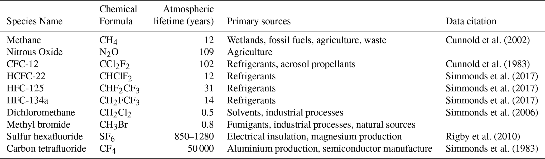
Cunnold et al. (2002)Cunnold et al. (1983)Simmonds et al. (2017)Simmonds et al. (2017)Simmonds et al. (2017)Simmonds et al. (2006)Rigby et al. (2010)Simmonds et al. (1983)

Table 3 Atmospheric species used in this study. Atmospheric lifetimes are taken from Burkholder et al. (2023). Primary sources are from Laube et al. (2022), Liang et al. (2022). References describing the AGAGE mole fraction data are provided for some species in addition to Prinn et al. (2018, 2025).

When calculating the monthly averages from the baseline-labelled observations, the influence of false positives and false negatives is strongly muted. This is demonstrated in Fig. 4, which shows that for almost all months, the error in the MLP model-calculated HFC-134a monthly mean at Mace Head and Gosan is substantially smaller than the baseline variability (1σ standard deviation in the baseline) within a month. Where outliers occur, these tend to be during months where there were relatively few data points, meaning that any mischaracterisation of the baseline can have a disproportionate influence.

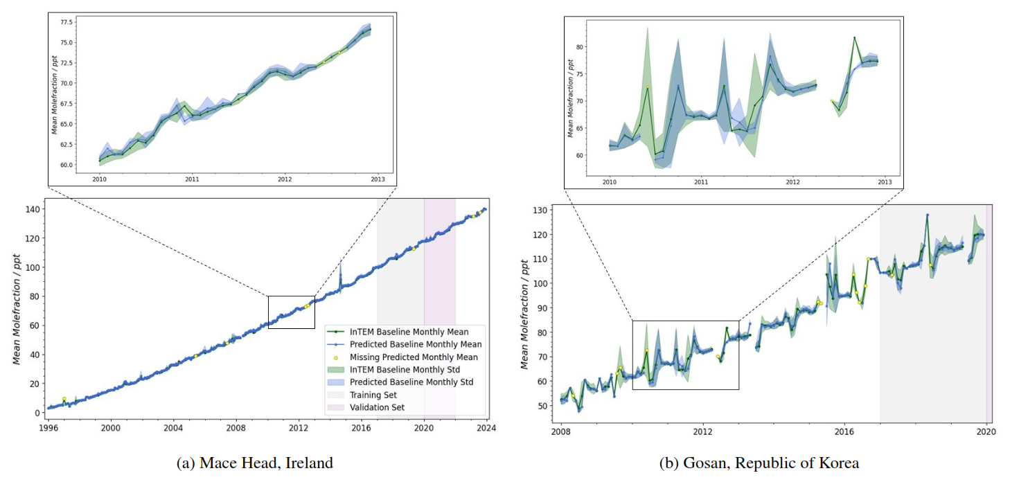
Figure 4 Baseline monthly means for HFC-134a at (a) Mace Head, Ireland; (b) Gosan, Republic of Korea. The NAME/InTEM baseline-derived values are represented by the green line, with associated 1σ variability within each month shown as green shading. The blue line shows the monthly means of data points that the MLP model classified as representative of baseline conditions. The 1σ variability within the model predicted monthly means is shown as blue shading. A subset of the dataset is shown in more detail in the top panels. Missing months are shown by yellow dots, and arise when a given month has no observations predicted as baseline by the model.

The overall performance of the algorithm applied to each species is summarised in Fig. 5, which shows the percentage error in the MLP-based monthly mean when compared to the InTEM-based equivalent, which is treated as the absolute truth here.

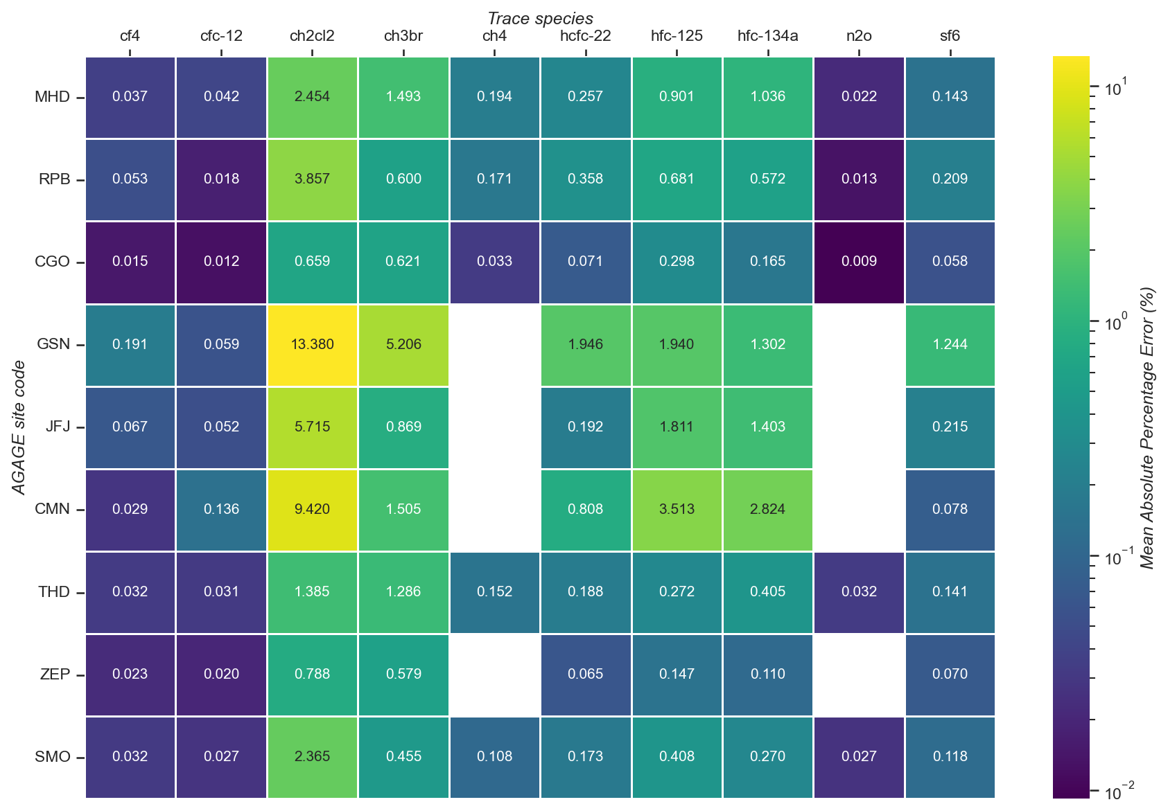
Figure 5 Mean Absolute Percentage Errors (MAPE) for the MLP model for selected AGAGE species across the nine monitoring sites. White denotes species that were not available at a particular site.

3.3 Coefficient of Variation and Model Utility

The CV metric demonstrates that variability in the true baselines is an indicator of model performance, as quantified by MAPE. As shown in the Supplement (Sect. S5), MAPE is generally higher for gases with high variability in their “true” baselines, compared to those with smaller CV. The smallest values of CV are associated with compounds that have relatively small gradients in the background atmosphere (e.g. CFC-12, N₂O). Shorter-lived compounds such as dichloromethane, which tend to exhibit substantial seasonal variability and zonal gradients, tend to show the highest variability in their true baselines. This pattern is observed across all sites. We therefore recommend caution when applying the method to species with a high CV relative to other species at the same site.

3.4 Computation and expected use cases

The computational cost of our baseline classification model is negligible compared to the calculation of LPDM footprints; on a standard desktop computer, the models consistently took less than a minute of wall time to train (3 years of data). Prediction of 1 year of baseline flags for ∼ hourly data, for the most part, takes less than 10 s. This should be compared to the calculation of LPDM footprints, which takes approximately 10 core minutes for each data point (the calculation of a year of baseline flags by combining the LPDM footprints and a tracer flux field is on the order of seconds to minutes of core time). The proposed ML surrogate is therefore approximately five orders of magnitude faster than the full-physics approach.

For very long time series, such as those presented in Figs. 1 and 4, the main cost associated with our model is the retrieval of subsets of meteorological analyses, which can take a substantial time due to network and storage latency from some archival services (although, of course, substantially larger data volumes are required to run the LPDM).

The envisaged use-cases for the ML algorithm are partly related to its small computational cost, and partly related to its ability to categorise baselines without the need for LPDM simulations. For example, we envisage that this algorithm can be built into data visualisation and quality assurance software, so that mole fraction baseline trends can be examined by data owners with low latency. This is compared to the current situation, in which LPDM runs need to be performed and integrated into the software, often by different research teams to those making the observation data, and often delayed by the availability of appropriate archived meteorology. These lags in the system can delay the analysis by weeks to months. Furthermore, our algorithm allows us to calculate baseline trends further back in time than is currently possible; at present, footprints have been calculated with NAME from 1989 onwards, and it would require a major resourcing effort (both in terms of staff time and computation) to extend these model runs to the beginning of the AGAGE record (1978). Datasets such as ERA5 cover this period and earlier, and can be used in the model prediction step. Finally, we envisage that this algorithm can be used to extend tracer-based methods beyond the period during which measurements were made. Consider, for example, a campaign in which ²²²Rn was used to derive baseline flags for one year at some location. Our algorithm can use these measurement-based flags in place of the NAME runs, and then be used to provide consistent flagging indefinitely beyond the study period.

These expected benefits must be weighed against the limitations of the model. Whilst we anticipate that improvements in the model architecture or training will be possible, it will always be an approximation of the training data, which is itself, in this case, model-based. Therefore, categorisation errors occur in the form of false positives (points labelled as baseline that are not), or false negatives (baselines that are missed), and so the algorithm should not be used if a precise categorisation is needed of a small number of samples. However, if aggregating over multiple measurements, for example, when calculating a monthly mean of ∼ hourly data, we have shown that the model has high skill in the majority of cases.

4 Conclusions

We have presented a neural network-based model for baseline air mass classification, based only on meteorological data. The model preserves many of the benefits of LPDM footprint-based classification methods, but at a fraction of the computational cost. Precision values of around 0.6 or higher were achieved for most sites examined here, and baseline monthly means were retrieved with uncertainties that were, in most cases, substantially smaller than baseline variability. We propose that this model can add value in low-latency data analysis and for extending baseline categorisation to time periods for which model simulations or co-measured tracers are not available.