Modelling wetland methane emission estimates by leveraging new observations of anthropogenic point-source plumes

Satellite retrieval capabilities for detecting methane (CH₄) diffuse and point sources have increased drastically over the last decade. These observations are playing an important role in atmospheric inversion systems to optimize emissions from anthropogenic and natural sources. A critical component of atmospheric inverse modelling is the prior estimate of CH₄ emissions, which impact both the magnitude of posterior emissions and the allocation between sectors, including wetland emissions. Here we incorporate point source retrievals from GHGSat to update prior emission estimate for fossil fuels. We then evaluate the effect on posterior emission using the Integrated Methane Inversion for the Western Siberian Lowlands. The updated GHGSat-informed fossil prior is highly uncertain but suggests the possibility of a reduction in wetland CH₄ flux. The approach demonstrates the potential impact of large point sources, that are typically not accounted for in bottom-up emission inventories. Due to modelling approaches adjusting anthropogenic and natural sources at the state vector level, the relative proportions of these sectors in the prior are critical for interpreting regional methane budgets and the effect of climate change on wetland emissions.

1 Introduction

Methane (CH₄) is a greenhouse gas, approximately 80 times as potent as CO₂ over 20 years, with a short atmospheric lifespan of approximately nine years, making it a target for climate mitigation efforts (Shindell et al., 2024). Aquatic and wetland ecosystems generate up to half of global CH₄ emissions (Rosentreter et al., 2021). While aquatic and wetland sources remain significant, recent budgets allocate more of these emissions to anthropogenic sources through eutrophication, reservoir emissions, and warming (Jackson et al., 2024). Despite reductions in methane attributed to aquatic and wetland ecosystems they remain the greatest uncertainty in global budgets (Saunois et al., 2025). These natural CH₄ emissions are potentially increasing with warming (Peng et al., 2022; Zhang et al., 2023).

Remote sensing approaches are critical for improving the monitoring, reporting, and mitigation of CH₄ emissions (Conrad et al., 2023). New technologies and the deployment of satellite constellations are increasing our ability to monitor super-emitters from various point sources, including oil, gas, coal mines, landfills, and agriculture (Jervis et al., 2021). The capacity for satellite-based remote sensing of these point-sources has increased significantly over the past decade with many satellites launching and entering operational status (GHGSat, NASA EMIT, GaoFen-5, MethaneSat, CarbonMapper; Jacob et al., 2022; He et al., 2024; Thorpe et al., 2023). Our methodology, using point source data from satellites to improve prior emission estimates is applicable beyond wetlands to any sector or region where emission sources spatially overlap, as demonstrated by similar approaches for Algeria (Naus et al., 2023) and globally (East et al., 2025). This study employs the Western Siberian Lowlands as a case study for the extrapolation of observed emissions to regional priors. Furthermore, the incorporation of plume estimates into the methane inversion modelling can improve our understanding of potential sectoral misattribution between anthropogenic and wetland methane sources. While point source satellite monitoring approaches are limited to high concentration anomalies from anthropogenic sources, the data can be combined with atmospheric inversions to improve estimates of natural sources.

1.1 Challenges in separating wetland and anthropogenic CH₄ emissions

In this study, we develop an approach to incorporate point source emissions into an atmospheric inversion model to improve estimates of wetland emissions for the Western Siberian Lowlands (WSL). In situ observations in WSL show CH₄ emissions from permafrost increasing during the thaw season (Rößger et al., 2022). However, ground measurements are sparse due to the region's large extent and remoteness. Globally, we calculated the overlap between wetlands and waterbodies and individual oil and natural gas fields using the Oil and Gas Infrastructure Mapping dataset (OGIM 1.1) and the Global Lake and Wetland Dataset (GLWD 2.0; Omara et al., 2023; Lehner, 2025; Fig. S1 in the Supplement). We found that 75 % of oil and natural gas fields have wetlands or water within their extent and on average 35 % (SD: 41 %) of individual oil and natural gas field area is wetland land cover. In Russia this rises to 98 % of oil and natural gas fields being co-located with wetlands and an average of 73 % (SD: 38 %) of individual oil and natural gas field area is classified as wetlands. In the WSL, wetlands and oil and gas facilities are highly likely to overlap. Wetland CH₄ emissions are diffuse, meaning that the emissions at any one location are very low compared to point sources. Still, if the wetland areas are large their emissions can result in considerable integrated fluxes per region. Therefore, modelling and satellite observations are necessary to understand regional CH₄ flux. Wetland CH₄ emissions are estimated using a “forward model”, i.e., chemical-transport model that predicts emissions, or from an `inverse model' using atmospheric inversions. Both approaches have large uncertainties due to limited data. Atmospheric inversions require a priori information on anthropogenic and natural emission sources with the large uncertainty of these estimates affecting the posterior flux estimates. Improving the prior flux estimate for anthropogenic sources using point source emissions data could thus potentially improve the posterior estimate of wetland emissions.

Russian oil and gas sector CH₄ emissions from atmospheric inversions are highly uncertain due to differing reporting methodologies, low observation density, and high variability between inventories (Shen et al., 2023). These emissions are estimated by sector primarily from the International Energy Agency and the United Nations Framework Convention on Climate Change (UNFCCC) for the Emission Database for Global Atmospheric Research (EDGAR) and the Global Fuel Exploitation Inventory (GFEI), respectively (Crippa et al., 2021; Scarpelli et al., 2022). These data are then spatially distributed to oil and gas infrastructure on a 0.1° × 0.1° grid globally. Bottom-up inventories such as Climate TRACE, GFEI, and EDGAR use the best available geospatial data to estimate the spatial distribution of emissions from various sectors, for example, oil refineries (Janssens-Maenhout et al., 2013; Scarpelli et al., 2022). For 2019, GFEI v2 has slightly lower oil, gas, and coal emissions compared to EDGAR v6.0 (Scarpelli et al., 2022). Some of the oil and gas infrastructure locations in Russia are restricted from the public domain (Omara et al., 2023). The uncertainty and lack of data completeness increase the likelihood of under attributing emissions to the oil and gas fields of the WSL, and over attributing emissions to natural sources such as wetlands. The Integrated Methane Inversion (IMI) provides a unified modelling framework for optimizing modelled CH₄ emissions with the TROPOMI methane (XCH₄) total column Level 2 data product (Copernicus Sentinel-5P, 2021; Varon et al., 2022a). The relative contribution of CH₄ from different sectors remains unchanged between the prior and posterior emission estimates at the level of state vector. Total annual emissions are optimized based on the TROPOMI XCH₄ observations. Therefore, when the proportion of emissions from sectors in a state vector element is incorrect, this will result in sectoral misattribution of emissions. This makes the distribution and relationship between sectors critical especially in regions with multiple high emission sectors such as the WSL.

1.2 GHGSat to inform CH₄ inversions

In this study, we use GHGSat data, a commercial satellite constellation that monitors super emitters, i.e., point sources with high emission rates (Brandt et al., 2014; Duren et al., 2019; Cary, 2006). GHGSat uses a Fabry–Pérot imaging spectrometer to monitor CH₄ absorption bands in the short-wave infrared (SWIR; Jacob et al., 2022; Jervis et al., 2021). Independent verification studies show GHGSat satellites have an emissions detection threshold of between 100–200 kg CH₄ h⁻¹, depending on the observation conditions (McLinden et al., 2024). In a controlled release study GHGSat detected a 400 kg CH₄ h⁻¹ plume (Sherwin et al., 2024). We develop a methodology to update regional oil and gas priors with plume measurements from GHGSat. GHGSat observations were acquired over three areas of oil and gas infrastructure in the WSL, as part of the NASA Commercial Satellite Data Acquisitions program's GHGSat evaluation. We apply our approach to the WSL, a region with extensive wetlands and oil and gas production.

2 Methodology

A database of GHGSat observations for the Western Siberian Lowlands (WSL) is developed and used to estimate prior anthropogenic emissions for the region. The updated priors are derived from the GHGSat emissions and geospatial information on the distribution of oil and gas infrastructure in the region. These updated emissions are incorporated into the IMI model and compared to default model simulations to determine the effect that unobserved emissions could be having on anthropogenic and wetland emissions in the region.

2.1 Study site

The WSL is a region of Russia with an estimated peatland extent of 592 440 km² and stores 70.21 Pg C in a mix of wetland and permafrost soils (Sheng et al., 2004). The region is important in the global carbon cycle, with a yearly emission from permafrost lakes estimated at 12±2.6 Tg C yr⁻¹ (Serikova et al., 2019). The WSL is within the Urals Federal District which is responsible for most oil and gas production in Russia (Suslov et al., 2019). Russia is the second largest emitter of fugitive CH₄ emissions from oil and gas (Solazzo et al., 2021) with ultra-emitters (>25 000 kg h⁻¹) estimated to represent between 10 % and 20 % of annual reported oil and gas emissions (Lauvaux et al., 2022). We define the model domain with a bounding box of 60.0 to 66.0° E and 70.0 to 79.1° N for a total area of 446 730 km². The IMI model setup includes optimizing the boundary conditions for 4° around each of the four sides of the model domain. The core domain includes the three GHGSat observation sites (Fig. S2)

2.2 Integrated Methane Inversion Model

We use the IMI model, based on the Goddard Earth Observing System (GEOS)-Chem (Henze et al., 2007; https://doi.org/10.5281/zenodo.4618180) and the Harmonized EMissions Component module (HEMCO; Lin et al., 2021). The chemical transport (CTM) model is optimized with TROPOMI XCH₄ using an analytical minimization of a least-squares Bayesian cost function (Varon et al., 2022a). Default priors were used in all cases besides oil and gas for our updated prior model. State vector clustering options included k-means clustering as the method, 100 as the max number of clusters, and 64 as the max cluster size. Uncertainty was estimated by running both the updated priors and default models three times, each with a different set of prior and observation error parameters: 0.75 and 0.2, 0.5 and 0.15, and 0.25 and 0.1, respectively. This results in accuracy metrics such as Root Mean Square Error (RMSE) and bias comparing the prior representing the CTM before optimization and the posterior representing the estimate following the optimization process to the TROPOMI observations. The priors for global modelling included in the IMI are (1) fuel exploitation from Global Fuel Exploitation Inventory (GFEI v2.0, Scarpelli et al., 2022), (2) other anthropogenic emissions from EDGAR v6.0 (Crippa et al., 2021), (3) geological seeps (Etiope et al., 2019), (4) fires (Randerson et al., 2018), (5) termites (Fung et al., 1991), (6) wetland fluxes from WetCHARTS (Bloom et al., 2017). To update these priors to include an estimate of fugitive emissions, we acquired GHGSat emission rates, a level 4 data product, as part of the NASA Commercial Satellite Data Acquisition onboarding review for the data. We downloaded data from the GHGSat platform SPECTRA (spectra.ghgsat.com/map). We requested GHGSat images for areas where oil and gas facilities are co-located with wetlands, specifically, the North Slope of Alaska, the Mississippi Delta, the Sudd Wetlands, the Niger Delta, and the Western Siberian Lowlands (WSL; Table S1). For this analysis, we used a total of 40 images acquired over three sites in the WSL (Fig. 1). The GHGSat constellation (in total, 12 satellites) targeted the three sites which each included multiple oil and gas facilities. GHGSat acquired at least ten images for all sites (n=13, 16, and 11). Sites 2 and 3 had images with multiple plumes within a single image (Table S2).

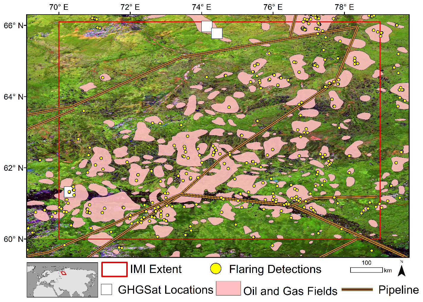
Figure 1 Oil and Gas infrastructure represented by gas flaring, oil and gas field extent, and pipeline locations for the WSL from the OGIM (Omara et al., 2023). The IMI model domain is in red and includes both all three GHGSat sites. MODIS surface reflectance composite displayed using R = band 7 (2105–2155 nm), Green = band 5 (1230–1250 nm), and Blue = band 3 (459–479 nm). All rights reserved. MODIS data courtesy of NASA LAADS DAAC.

2.3 Updating oil and gas priors

To update the oil and gas priors, we created a fugitive emissions distribution and combined that with the default fossil fuel prior. To create the spatial distribution of fugitive emissions, we used a combination of GHGSat plume emissions and oil and gas flaring detections from OGIM (Omara et al., 2023) extrapolating GHGSat emission estimates to oil and gas infrastructure locations that were not observed in our GHGSat acquisitions (Fig. S3). Flaring locations were utilized as a proxy for oil and gas infrastructure due in part to their previous utilization to develop geospatial information on oil and gas field locations (Zhang et al., 2020). We did not utilize infrastructure datasets as they are incomplete for the region, and oil and gas fields were not used as that would have distributed emissions to areas not in active production.

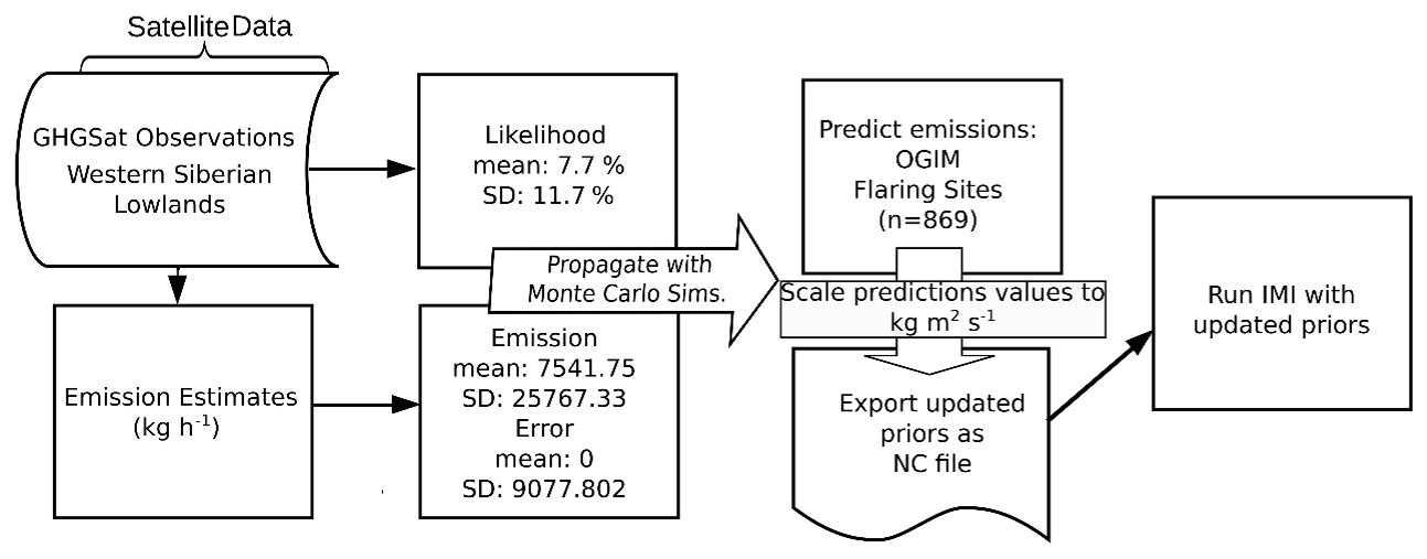
The GHGSat plume detections were assumed to represent a statistical sample of leaking infrastructure that can be extrapolated to all oil and gas facilities, represented by flaring detection, in the region. In the WSL, we observed 20 plumes for the 40 image acquisitions, including three images with two plumes from two different facilities (Table S2). Satellite acquisitions targeted three areas of the Western Siberian Lowlands from July 2023 to April 2024 as part of the NASA CSDA Programs assessment of GHGSat. We utilized the propagate package (Spiess, 2018) in R Statistical Software 3.6.3 (R Core Team, 2021) to estimate the annual CH₄ emissions for all flaring locations, the best available proxy for the distribution of oil and gas infrastructure in the region available from OGIM. The error propagation Eq. (1) combined emissions, emission error, and likelihood along with each terms associated uncertainty (Eq. 1):

$$\begin{array}{}\text{(1)}& \begin{array}{rl}& \mathrm{average}\mathrm{emission}\mathrm{per}\mathrm{oil}\mathrm{and}\mathrm{gas}\mathrm{infrastructure}\left(\mathrm{kg}{\mathrm{h}}^{-\mathrm{1}}\right)\\ & =\left(\mathrm{Emissions}\pm \mathrm{Error}\right)\times \mathrm{Likelihood}\end{array}\end{array}$$

The emissions term was calculated as the average of all reported plume emission rates and uncertainty is the standard deviation (Table S2). Plume emissions rates are a level 4 data product provided by GHGSat and calculated using the integrated mass enhancement (IME) method (Varon et al., 2018). The IME method provides error estimates with the major source of error being the windspeed especially in areas like the WSL where modelled windspeed is utilized (Varon et al., 2018). The plume estimates in this study utilized GEOS-FP for windspeed except the acquisition on 12 March 2024 which utilized Meteoblue for windspeed. The average of all errors and standard deviation was used as the error term (Table S2).

Finally, emission likelihood was calculated by first identifying all oil and gas infrastructure within each GHGSat footprint from high resolution imagery. We considered the occurrence of emissions at each site relative to the number of facilities and image acquisitions. To calculate the likelihood of emission occurrence, we first identified the number of oil and gas facilities within each site's satellite observations footprint. The oil and gas facilities at each site were 18, 27, and 6 for site 1, site 2, and site 3, respectively. The oil and gas facilities per site were then used to calculate the rate of occurrence (Eq. 2):

$$\begin{array}{}\text{(2)}& \begin{array}{rl}& \mathrm{Site}\mathrm{rate}\mathrm{of}\mathrm{occurrence}\\ & ={\displaystyle \frac{\mathit{\#}\mathrm{of}\mathrm{observed}\mathrm{plumes}\mathrm{at}\mathrm{the}\mathrm{site}}{\mathrm{Total}\mathrm{Facilities}\mathrm{at}\mathrm{the}\mathrm{site}\ast \mathrm{Total}\mathrm{Observations}\mathrm{of}\mathrm{the}\mathrm{site}}},\end{array}\end{array}$$

For example, site 1 had 12 satellite acquisitions, 2 detected plumes, and 18 structures identified as potential oil and gas infrastructure. This resulted in an estimate of two detected plumes out of a possible 216 observations of infrastructure or a little less than a 1 % chance of observing an emission at the site. The mean and standard deviation of the emissions, error, and likelihood terms were propagated using matrix calculus of the covariance structure and 100 000 Monte Carlo simulation using a Gaussian copula with marginal t-distributions (Spiess, 2018) . We treated each flaring location as a proxy for a complex of oil and gas infrastructure, consistent with the GHGSat observation sites. All flaring detections from the OGIM including locations within the model domain and those within the 4° boundary region were used as possible emission sites (n=869; Fig. 1). OGIM oil and gas flaring detections use VIIRS data which has a 750 m spatial resolution making facility clusters a likely occurrence, therefore we consider these sites to be analogous to our GHGSat observation sites and the likelihood for entire sites is applied to flaring sites. The annual emissions for each of the 869 sites were estimated using a random normal distribution of the mean and standard deviation from the Monte Carlo simulations (Fig. 2). Any negative values resulting from this prediction were assumed to be zero emissions, i.e., non-occurrence. We converted these values into a NetCDF file and incorporated this updated prior into the IMI as an additional fossil fuel emission in the oil and gas prior estimate (Fig. 2).

Figure 2 The workflow for updating oil and gas priors with GHGSat from plume observations.

2.4 Integrated methane inversion (IMI) model runs

The IMI v1.2.1 was run following standard methods on Amazon Web Services (AWS) (Varon et al., 2022a, b). We ran a default model (with GFEI v2.0 fossil fuel priors) and another model with GHGSat informed priors, subsequently referred to as the default and updated models, respectively. The IMI uses GEOS-Chem, a chemical transport model, as the forward model to constrain CH₄ fluxes based on the coal, oil, and gas priors from GFEI v2.0 and other anthropogenic priors from EDGAR v6.0 (Varon et al., 2022a).

We ran the model from 1 June to 31 July 2021 with a model spin up from 1 to 31 May 2021. We ran a nested grid simulation for the WSL region (60–66.1° N and 70.0–79.0° E). Despite a short model run there were 121 591 TROPOMI XCH₄ observations, which we deemed adequate for our study goals. This domain resulted in a total of 733 state vector elements at a 0.25° × 0.3125° spatial resolution, which were then clustered into 100 elements. The different priors would result in each model having unique state vector clusters. To control for this variability, we used the state vectors from the updated model for both model runs. All other parameters were set to the default except the updated model, which included the GHGSat-derived emission layer in the priors.

3 Results

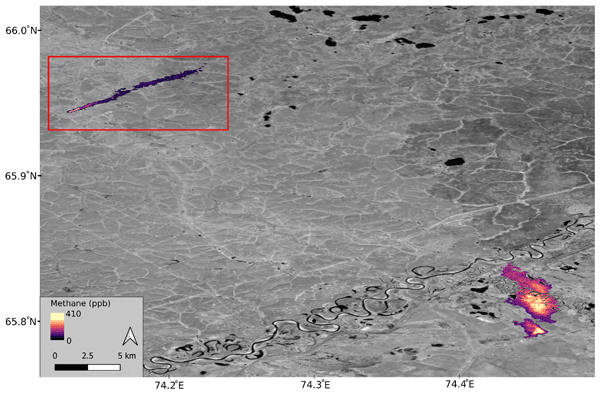
The average CH₄ emission from the GHGSat plume detections was 7541±25 767 kg CH₄ h⁻¹. The smallest observed plume had a rate of 378 kg CH₄ h⁻¹. The median of our observed plumes was 946 kg CH₄ h⁻¹. The largest observed emission was 116 739 kg CH₄ h⁻¹ in site 1, which was one of only two plume observations at that location (Table 1). In contrast, site 3 had consistently smaller magnitude plumes in all but one image. At site 3, emissions averaged 2124±2082 kg CH₄ h⁻¹. The observation on 20 April 2024 was site 3's second-largest observation (Fig. 3).

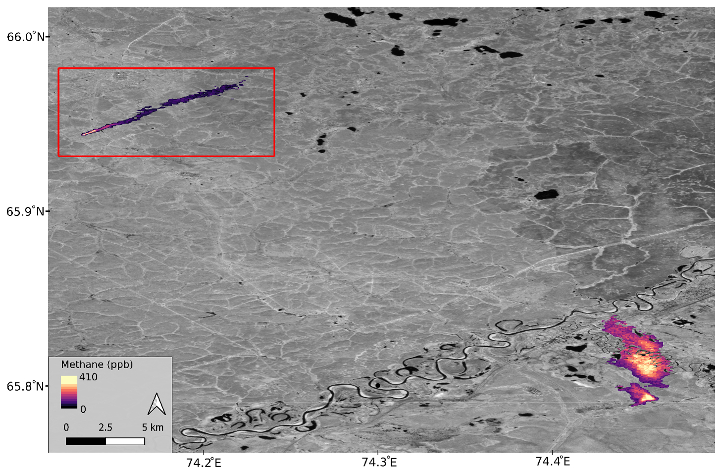
Figure 3 Plume observations from two oil and gas sites in the Western Siberian Lowlands near Pangody, RU. The northern plume (denoted by the red box) was observed on 12 March 2024 at 09:47:13 at an estimated rate of 1873±917 kg CH₄ h⁻¹. The plumes in the southeast of the figure were observed on 20 April 2024 at 09:30:59 at an estimated rate of 2694±1050 kg CH₄ h⁻¹ and 4596±1792 kg CH₄ h⁻¹. The impact of the river on the southern plume is evident with no methane concentration for those pixels. Background image is PlanetScope panchromatic (band 8) ©Planet Labs PBC. All rights reserved. The plumes in the image are derived from GHGSat imagery ©GHGSat. All rights reserved.

3.1 Updated priors

Emissions were estimated for 452 of the possible 869 facilities within the model domain and 4° boundary region of which 158 were within the model domain. Our probabilistic emissions increased the oil and gas prior by 4.48 Tg CH₄ yr⁻¹ in the model domain (Fig. 1). The GFEI v2.0 estimates coinciding with the GHGSat observation sites were 3.973×10⁵, 3.210×10⁶, and 2.4×10² kg CH₄ yr⁻¹ for site 1, site 2, and site 3, respectively. If scaled to annual values (assuming year-round flux), the GHGSat observation estimates for each site are 9.4458×10⁷, 1.355×10⁶, and 2.004×10⁷ kg CH₄ yr⁻¹ for site 1, site 2, and site 3, respectively. Sites 1 and 3 were orders of magnitude larger than the GFEI estimates.

The likelihood of occurrence calculation resulted in occurrence rates for each site of 0.93 %, 0.93 %, and 21.2 %, which we averaged resulting in a 7.7±11.7 % likelihood of occurrence across the three sites (Eq. 2). If a single rate of occurrence is calculated for all sites the occurrence rate falls to 2.8 %. Emission and error terms were calculated from the GHGSat plume emission and error estimates resulting in CH₄ emission values of $\mathrm{7},\mathrm{541.8}\pm \mathrm{25}$ 767.3 kg h⁻¹ and CH₄ emissions error of 0±9077.8 kg h⁻¹. Following the propagation of these error terms using Eq. (1), we found a mean of 792 kg h⁻¹ and standard deviation of 4032 kg h⁻¹ (0.22 SD 1.12 kg s⁻¹). According to the GFEI v2.0, oil and gas emissions are 0.57 Tg CH₄ yr⁻¹ within our study region (Scarpelli et al., 2022). The likelihood calculation was then applied to all flaring locations, resulting in 56.6 % of the 869 facilities having modelled annual emissions greater than zero. In the IMI domain, 158 of the 305 flaring detections had emissions. These updated emissions estimates resulted in a 4.48 Tg CH₄ yr⁻¹ estimate of plume emissions in the domain and a total prior emission estimate of 7.2 Tg CH₄ yr⁻¹. Our updated prior resulted in a significant increase in oil and gas emissions.

3.2 IMI emissions and performance

Our updated prior increased total prior emissions from 2.7 to 7.2 Tg CH₄ yr⁻¹. The updated model resulted in a total posterior emission estimate of 2.98 Tg CH₄ yr⁻¹ (2.92–3.18 Tg CH₄ yr⁻¹). The default scenario had a slightly lower total posterior emission estimate of 2.71 Tg CH₄ yr⁻¹ (2.64–2.91 Tg CH₄ yr⁻¹). The total posterior estimates were very similar, given that they used the same TROPOMI data as an atmospheric constraint (Fig. 4). However, the posterior estimates were outside each other's uncertainty. The wetland CH₄ prior in both IMI models was 2.23 Tg CH₄ yr⁻¹. The posterior wetland emissions in the default model fell slightly to 2.22 Tg CH₄ yr⁻¹. In contrast, the run using the updated GHGSat priors resulted in the posterior wetland emission falling to 1.6 Tg CH₄ yr⁻¹ (Fig. 4).

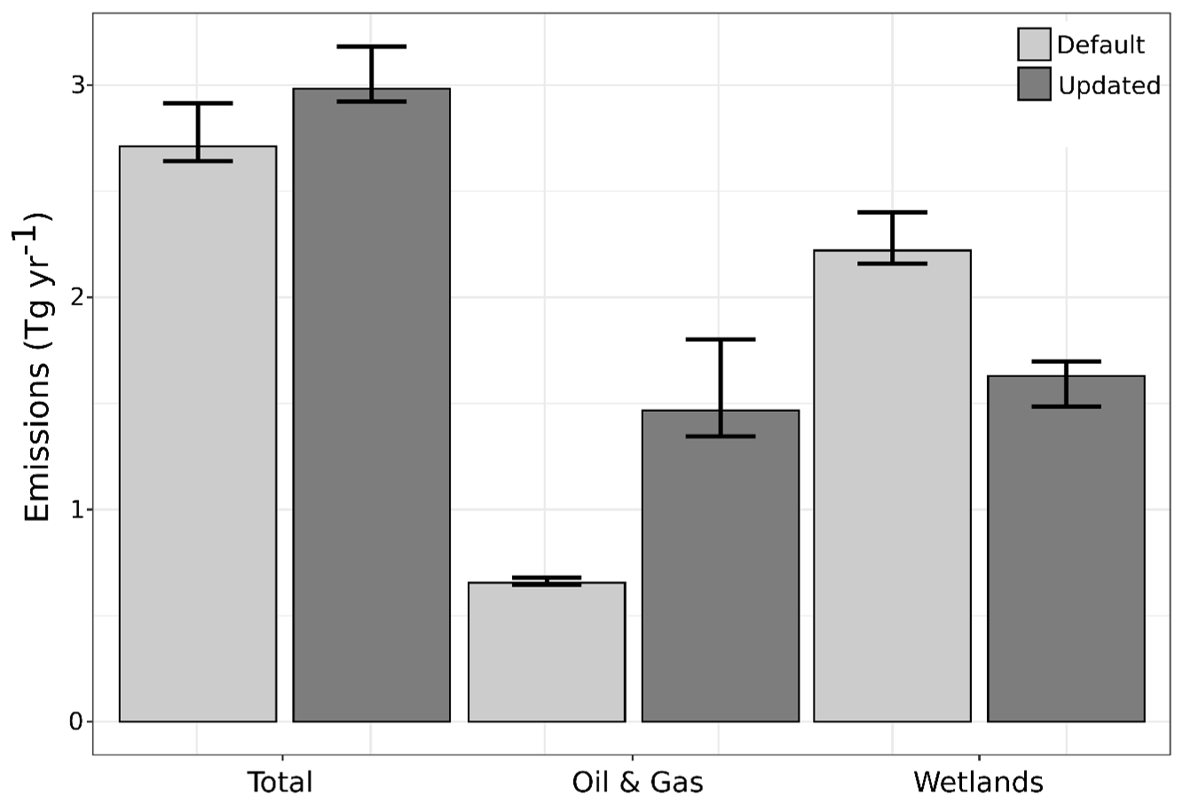
Figure 4 Posterior flux estimates for total emissions, oil and gas, and wetlands from both default and updated model runs, scaled to represent annual totals. Values scaled to the actual model run period (1 to 31 July 2021) are shown in Fig. S4.

The updated model's higher prior emissions resulted in an increase in degrees of freedom. The posterior estimate from the inversion using the GHGSat updated priors had a slightly larger negative bias when comparing the posterior simulated CH₄ concentrations from GEOS-Chem to observed XCH₄ from TROPOMI (Table 1). Both models had improved performance in the posterior RMSE compared to the prior RMSE. For our domain there were 35 906 super-observations, representing 121 591 TROPOMI XCH₄ observations. The averaging kernel sensitivity demonstrates that a few of our GHGSat informed priors are in locations that are unlikely to have emissions of that magnitude, which results in very low-scale factors. The model optimizes emissions estimates by comparing prior driven GEOS-Chem outputs to TROPOMI XCH₄ observations. If the TROPOMI estimates are substantially different than the modelled, a scaling factor is applied to align the modelled emissions with the TROPOMI data. Therefore, a low-scale factor occurs when TROPOMI emissions are low, and the modelled emissions are high. The major difference in the two models is the large northern regions, which have high scale factors in the default model and lower scale factors in the updated model. The updated model's inclusion of fugitive emissions in these regions results in (1) lower scale factors and (2) less of the regions emissions attributed to wetlands (Fig. 4). Both models agree that a low scale factor is appropriate for the southern portion of the model domain (Fig. 5). This information could be used to update the distribution of our emission estimates and improve the updated model's performance. Low averaging kernel sensitivities approaching zero demonstrate where the model lacks TROPOMI XCH₄ observations to constrain the forward model (Fig. 5). Portions of the model domain had low sensitivity due to a lack of TROPOMI observations, which is a major uncertainty in this approach in regions with extensive wetlands and waterbodies.

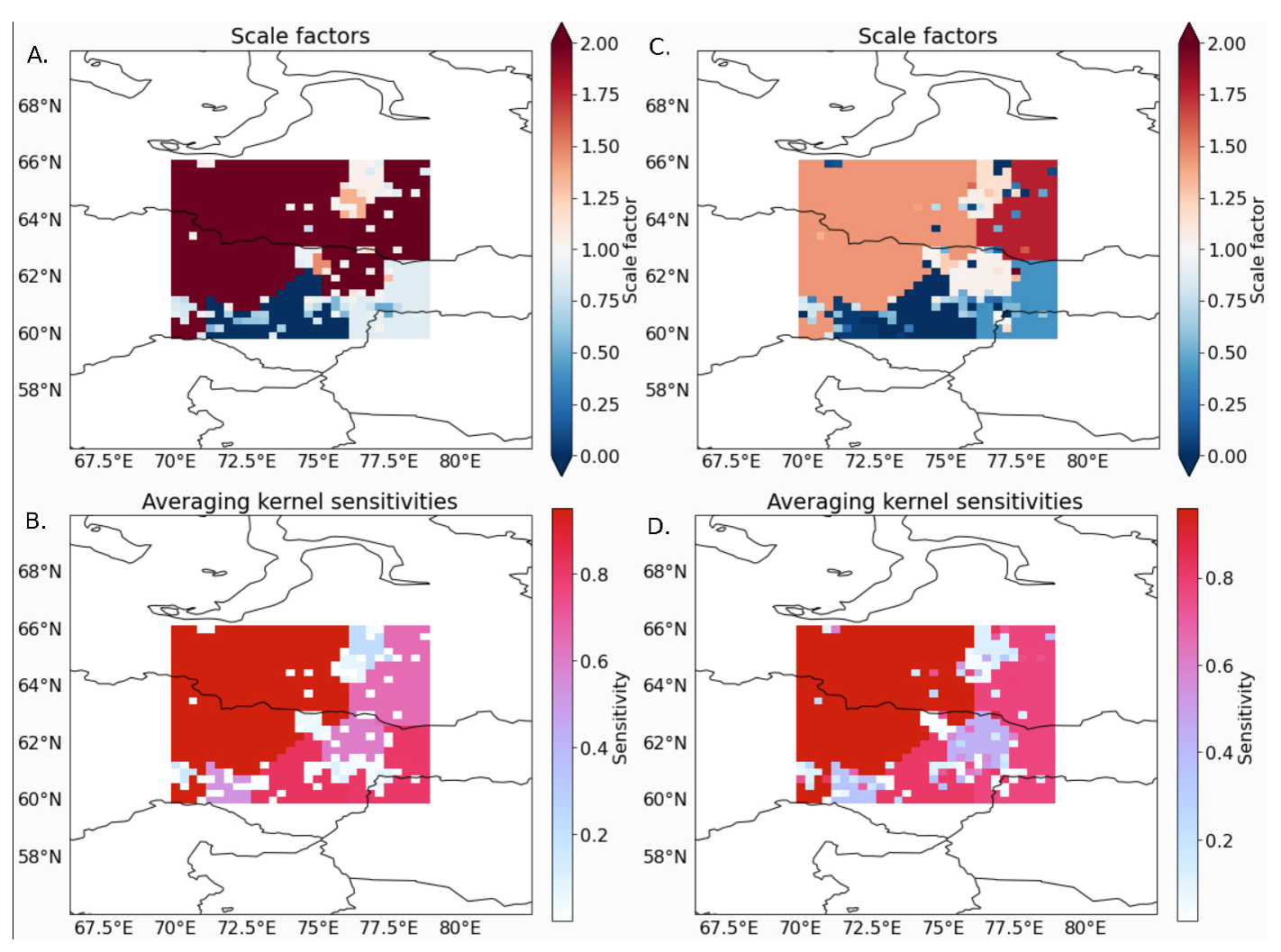
Figure 5 (A) The scaling factors for the default model. (B) the averaging kernel sensitivities for the default model. (C) Scaling factors for the updated model. (D) the averaging kernel sensitivities for the updated model.

Table 1 The mean bias and RMSE for the default and updated model run. Values are calculated by comparing the GEOS-Chem atmospheric column CH₄ concentrations to the observed TROPOMI XCH₄ (Figs. S5–S6).

4 Discussion

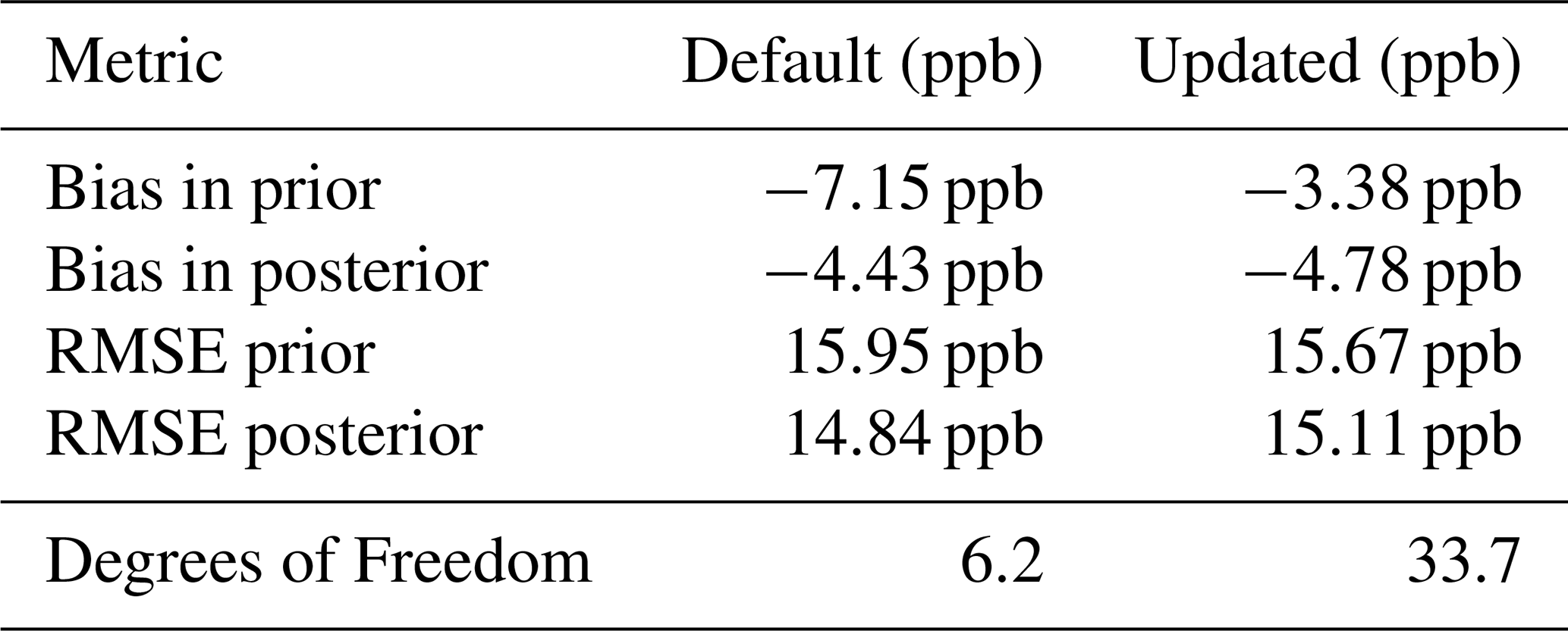
The bias and RMSE are calculated by comparing simulated CH₄ concentrations based on the prior emissions estimates to the observed TROPOMI CH₄ concentrations and simulated CH₄ concentrations using the posterior emissions estimates to the observed TROPOMI CH₄ concentrations for the model domain. The bias indicates that both prior and posterior GEOS-Chem model outputs were lower across the region than the TROPOMI XCH₄ observations (Table 1). The posterior simulations using the default and updated prior emissions estimates had similar biases of −4.43 and −4.78 ppb, respectively. The lowest bias was found between the prior GEOS-Chem simulation using the GHGSat and OGIM updated priors and the observed XCH₄ from TROPOMI. The failure of the inversion to improve on this in the posterior model suggests a disconnect between the spatial distribution of our updated priors, the TROPOMI XCH₄ observations, and the clustered state vectors. The bias metric illustrates that both prior and posterior emissions were consistently biased lower than the TROPOMI observations. The scale factors also demonstrate that individual elements with high updated emissions values were often scaled down, and in contrast many of the larger regional areas have the potential for higher methane emissions (Figs. S3, 5). The combination of clustering and extrapolation failed to capture the spatial pattern of emissions.

The posterior wetland emission estimates from the default and updated inversions were 2.22 and 1.63 Tg CH₄ yr⁻¹, respectively. The GHGSat informed priors resulted in a reduction of 0.59 Tg CH₄ yr⁻¹ attributed to wetlands. To put this in global context, this potential reduction represents 9.8 % of the increase in CH₄ emissions attributed to wetlands from 2019 to 2020 (6.0±2.3 Tg CH₄ yr⁻¹; Peng et al., 2022). This finding is highly uncertain, but our approach demonstrates that fugitive methane emissions from oil and gas exist across the region and correctly modelling their magnitude and spatial distribution would reduce the modelled wetland methane emissions. Previous studies utilizing plume estimates of super emitters with atmospheric inversion have found increased attribution of methane emissions to the oil and gas sector (Naus et al., 2023). The prior emissions estimate for oil and gas informed using additional high-resolution observations affects wetland posterior emission estimates illustrating the potential of plume mappers to constrain wetland emission estimates in areas where the sources are closely co-located. Our approach was limited by (1) an overestimation of the magnitude of the updated prior, which was adjusted for by the atmospheric constraint, (2) uncertainty in the spatial distribution of new emissions. Our approach demonstrates potential but needs more data to reduce the uncertainty.

4.1 Uncertainty

Our modelling approach has several major uncertainties. The GHGSat informed priors are based on limited data from three sites across a region with extensive oil and gas facilities. It is possible that our observation sites are not representative of the region's oil and gas infrastructure. For example, only one of our three observation sites had detected flaring in the OGIM database. Additionally, less flaring has been linked to increased venting of excess gas (Irakulis-Loitxate et al., 2022), therefore, the flaring detections may underestimate potential emission sites and represent sites with consistent flaring but limited emissions. Pipelines are another source of fugitive emissions and were not included in our distribution of emissions. Additionally, our approach assumes consistent emissions across time, but fugitive emissions are sporadic and unpredictable in length and timing. In the Permian basin, on average 26 % of plumes were found to be persistent across multiple airborne deployments from September to November 2019 (Cusworth et al., 2021). Ideally, repeat coverage of the entire study domain would be available to determine plume persistence. However, regional plume observations are not available at the sensitivity of GHGSat. The IMI scaling factors are another uncertainty, optimized for only the period of interest from 1 June to 31 July 2021 but we use these values in calculating estimated emissions for the year. Running the model for the entire year would reduce this uncertainty. Shen et al. (2023) suggest that the low number of TROPOMI XCH₄ observations at high latitudes increased uncertainty in Russian inversions and that the GFEI 2.0 inventory underreported Russian emissions by a factor of two (2023). The posterior oil and gas estimate from the inversion using the updated oil and gas priors does represent approximately a doubling of the oil and gas emissions compared to the default inversion (0.65 to 1.47 Tg CH₄ yr⁻¹). Additionally, the default wetland and fossil priors are from 2017 and 2019, respectively, leading to some expected discrepancies between the modelled concentrations and TROPOMI XCH₄ observations in 2021.

4.2 Distribution of update priors

To propose an improved approach to spatialize and update plume derived priors we analysed annual 2021 TROPOMI XCH₄ in relation to ancillary data including the Global Impervious Surface Area (GISA-10m; Huang et al., 2022) and GLWD 2.0 (Lehner et al., 2025). We analysed average TROPOMI XCH₄ for 2021 by percent impervious surface and percent wetland bins of 0–10, 10–20, 20–30, 30–40, 40–50, 50–60, 60–70, 70–80, 80–90, 90–100 and by considering if the pixel fell within a gas field. We found that XCH₄ as observed by TROPOMI increased with impervious surface and decreased with wetland extent with both relationships being more pronounced in gas fields (Fig. 6). The strong relationship of impervious surface to increased XCH₄ in the region suggests that with additional refinement, impervious surface data could be more suitable than flaring to inform the spatial distribution of the updated priors. However, oil and gas infrastructure related disturbance has been identified as a driver of natural CH₄ emission hotspots (Sabrekov et al., 2022), which may contribute to the increasing TROPOMI XCH₄ relative to percent impervious surface. There is also the possibility that surface material is resulting in albedo-derived artifacts in the methane retrievals (Lorente et al., 2021).

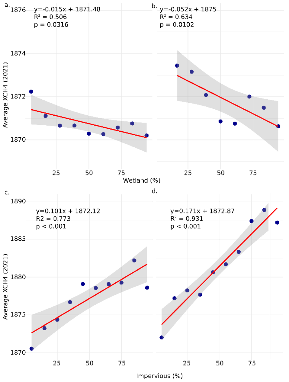
Figure 6 (a) The linear relationship of average XCH₄ to wetland extent bins for non-gas fields. (b) The linear relationship of average XCH₄ to wetland extent bins for gas fields. (c) The linear relationship of average XCH₄ to impervious surface extent bins for non-gas fields. (d) The linear relationship of average XCH₄ to impervious surface extent bins for gas fields.

Still, our work demonstrates the potential for improved modelling of CH₄ emissions from natural sources by incorporating plume-based mapping measurements in prior emission estimates. Oil and gas inventories for the region do disagree considerably by up to an order of magnitude (Scarpelli et al., 2022). Disagreement between GFEI v2.0 and Climate TRACE suggests that depending on tracking methodology, oil and gas emissions could be higher in the region. Still, our updated oil and gas priors are relatively high and would represent approximately 32 % of Russian emissions for 2022 (Reuland et al., 2024). The latest version of GFEI demonstrated that the magnitude of methane plume mappers poorly correlates with the GFEI 3.0 emission estimates (Scarpelli et al., 2025).

4.3 Satellite Remote Sensing of Methane Plumes

Fugitive emissions contribute to the uncertainty of emissions in the WSL. Plume mapping satellites are beginning to address this data gap (Jacob et al., 2022). The satellites with the capability to map plumes include NASA EMIT, GaoFen-5, GHGSat, Worldview-3, Sentinel-2, MethaneSat, TROPOMI, and Carbon Mapper. However, the use of these satellites for mapping plumes is limited by data access due to cost, expertise necessary for plume detection and emissions estimation, data processing, and sensor and mission limitations. For example, the WSL has limited collections from freely available datasets due in part to the low albedo in the SWIR of the peatland landscape limiting returns from coarse spatial resolution satellite sensors and the high latitude limiting acquisitions from EMIT which is on the ISS. In contrast, we found GHGSat plume observations were minimally impacted by wetlands and waterbodies in the WSL (Fig. 3). The GHGSat constellations did have a blackout season with no observations between approximately November 2023 and February 2024; for example, the last acquisition in the fall of 2023 was 2 November 2023 and the first in 2024 was 12 February 2024. These observations were for the WSL 2 site (61.3° N), with the higher latitude sites (65.8° N) having no observations in November or February (Table S2).

Earth observation solutions for improved monitoring of the WSL are currently limited. The SRON (Netherlands Institute of Space Research) plume dataset (Schuit et al., 2023) used TROPOMI data to map CH₄ plumes and found 18 plumes in our domain for 2021. The smallest was 4000 kg CH₄ h⁻¹, which is larger than all but three of the GHGSat detected plumes (Fig. S7). Carbon Mapper utilizing the Planet Labs Tanager satellite has also observed the WSL finding 110 plumes in our study area and identifying emission from 86 of them (Duren et al., 2025; Carbon Mapper, 2025, 2026). The smallest plume found was 217 kg CH₄ h⁻¹ and in general the magnitude of observed plumes was similar to GHGSats but across a much wider geographic scope (Fig. S7). The addition of these other datasets would remove much of the spatial bias we were trying to address with our extrapolation. The mean emission rate of the GHGSat plume data was 5.2 times less than the SRON data. In contrast, the average Tanager detected emission was 2183.9 kg CH₄ h⁻¹ compared to 7541.8 CH₄ h⁻¹ for GHGSat. Tanager's lower average emission rate could be due to the additional categories of CH₄ emissions being tracked by Tanager. The uncertainty was lower for the Tanager emissions. It is evident that consistent small emissions from oil and gas infrastructure in the WSL are common in our study sites and are not picked up by the plume mapping approach of the SRON dataset due to the spatial resolution and detection threshold of TROPOMI. While these emissions should be represented in the TROPOMI XCH₄ data, the limited returns in wetland, permafrost, and water pixels impact the robustness of these data in regions like the WSL, making accurate inventory data critical for these locations. The sensitivity of the GHGSat or Tanager observations (∼ 100–200 kg h⁻¹) and high spatial resolution (∼ 30 m) is crucial for this region, as it allows for the observation of smaller fugitive emitters that are interspersed with wetland environments. Global modelling efforts incorporating GHGSat observations found 32 % increase in oil and gas emissions over UNFCCC estimates (East et al., 2025). Their study demonstrates the potential of GHGSat for informing methane priors and constrains their analysis to 25×25 km areas where emissions were monitored making exploration of extrapolation, satellite data source synthesis, and localized methods focused on wetlands critical for informing future modelling.

Ideally, daily plume estimates for the entire region would be available and utilized to update oil and gas prior emission estimates. However, given the limited current data, our methodology uses plume emission data to improve estimates of wetland emissions. We considered using SRON's plume data to provide a regional estimate of plume occurrence but the instruments' differing sensitivities to CH₄ concentration complicates combining the two for improved estimation of the frequency of plumes across the region. While SRON's mapping effort examines mean emissions across the entire region, the super emitters observed are different from the smaller but persistent plumes observed by our study's GHGSat observations. Additional GHGSat images and other satellite data sources would improve our GHGSat informed priors' spatial distribution and emission estimates. The next step for this work would be to utilize all these available plumes (Tanager, SRON, and GHGSat) to update emission priors for the region and without extrapolation following a similar approach to Naus et al. (2023). A limitation of incorporating Carbon Mapper directly into our current approach is the lack of information on non-occurrence observation.

4.4 IMI and future work

The development of the IMI is an ongoing process, with v2.0 and v2.2 being released during our study. These new versions incorporate features that are directly relevant to our work, such as plume measurements from SRON (Schuit et al., 2023) and additional options for including TROPOMI XCH₄ data over water. We used v1.2.1 of the IMI to test the use of GHGSat informed priors in a stable modelling environment. The benefits of water tolerance are significant, given that 13 % of our domain is potentially water, as calculated from the global maximum extent surface water layer (Pekel et al., 2016). The gaps in TROPOMI XCH₄ observations due to water and wetlands limit the ability of the IMI to constrain the forward model outputs in those locations (Fig. S8). This results in the inversion defaulting to the prior emission estimates in affected state vector elements, emphasizing the importance of accurate prior emission estimates from oil and gas.

IMI research so far has focused on utilizing analytical inversions to constrain fossil emissions at regional to global scales (Shen et al., 2023; Zhang et al., 2020, 2025). The utility of the approach is clear, however, the utilization of the IMI for improving our understanding of wetland environments has been limited but impactful (He et al., 2026). Utilizing GHGSat, we observed three locations in the WSL, finding consistent plume emissions at the observed facilities. We updated regional prior emission estimates with existing data on oil and gas infrastructure and plume emissions to constrain wetland emissions in the WSL. If oil and gas facilities across the model domain had similar emissions to those observed with GHGSat, then less wetland emissions are likely to have occurred in this region during the study period. As additional satellites launch and more plume emission data are collected, we will increase our ability to improve the accuracy of inverse modelling of atmospheric methane concentrations and reduce uncertainty in global wetland emission estimates.