Development and characterization of an advanced holographic instrument for atmospheric research

In this study, we develop and characterize an advanced holographic instrument – HOLODROPS (HOLOgraphic DROPlet Sensor). HOLODROPS operates in two configurations: (1) HOLODROPS, designed for long-term, high-precision measurements of cloud droplet size distributions, and (2) HOLODROPS-TRACK, designed for targeted, short-interval particle tracking to study turbulence and collision-coalescence processes. Unlike traditional optical scattering or imaging probes, both configurations can simultaneously capture the size, shape, and three-dimensional position of multiple droplets and ice crystals larger than 8.8 µm within a sample volume, eliminating the need for multiple instruments and yielding more accurate and cohesive data. However, the detailed three-dimensional particle tracking provided by HOLODROPS-TRACK requires significant computational resources for hologram reconstruction and data processing, limiting its use over extended measurement periods. To address this challenge, we developed a complementary event-based Particle Image Velocimetry (ePIV) system, which leverages an event-based camera to assess key cloud motion features in real time with substantially lower data volume and processing. ePIV provides continuous monitoring of fluid flows to identify optimal measurement windows and informs targeted deployment of HOLODROPS-TRACK, paving the road for efficient, high-resolution particle tracking when conditions are most scientifically valuable. All three systems have been successfully characterized and validated in the laboratory. Additionally, we successfully tested HOLODROPS in an outdoor setting during a drizzle event to demonstrate the prototype's adaptive operation.

1 Introduction

The study of atmospheric processes is closely linked to advances in instrumentation, as cutting-edge tools are essential for unraveling the atmosphere's complexities. Especially, clouds still contain many secrets that we need to uncover to fully understand the underlying processes and to improve both weather and climate predictions. To understand, for example, why some clouds rain and others do not, we need to accurately determine the internal structure of the clouds and the droplet size distributions, which can only be done with measurements using high-precision instruments in a cloud chamber or a real cloudy environment. Knowing the size distribution of cloud droplets helps explain precipitation since this depends on how liquid water is distributed among droplets. For example, smaller droplets of similar size tend to maintain the same velocity and rarely collide. While a broader distribution with larger droplets can collide through collision-coalescence, and once these droplets get large enough, drizzle forms (Lu et al., 2018).

Generally, advanced techniques can be divided into in-situ and remote sensing methods. For in situ measurements, the instruments are exposed to the cloudy environment to measure the concentration and phase of hydrometeors. Typically, individual droplets are measured, and a size distribution is determined after averaging over time. Counting statistics are typically sufficient to obtain meaningful size distributions within one second. This means that for an airborne instrument flying at 100 m s⁻¹, averaging over 100 m, and even for a ground-based instrument, the cloud can change significantly within that time.

For in-situ instruments, two main techniques are used: scattering and holographic or shadow imaging. Shadow imaging, as the name suggests, uses shadow images to determine the size and shape of each hydrometeor and to count them to obtain a size distribution. Holographic imaging uses a coherent light source to illuminate particles and capture the interference wavefront. For scattering, Mie theory is used (Lance et al., 2010). A droplet scatters light at a predetermined angle at a known intensity and thus can be sized when that intensity is measured. Again, individual droplets are measured to obtain the size distribution. Other techniques determine bulk cloud properties, such as liquid water content.

Remote sensing methods infer particle size distributions (PSDs) indirectly by measuring how aerosols, cloud droplets, ice, or precipitation scatter, absorb, emit, or reflect radiation. Active radar transmits microwave or millimeter-wave signals and measures the return signal; single-frequency radar primarily provides reflectivity, which is strongly weighted toward larger particles, whereas multi-frequency radar uses wavelength differences to better constrain the characteristic particle size and PSD shape. Doppler and polarimetric radar provide information on particle fall speeds, shapes, orientations, and hydrometeor types, improving PSD estimates for rain, snow, and ice. Passive methods, such as visible/near-infrared satellite imaging, thermal infrared sensing, microwave radiometry, sun photometry, and polarimetry, use natural solar or thermal radiation to estimate quantities like aerosol optical depth, cloud optical thickness, effective radius, liquid or ice water path, and fine/coarse aerosol modes. Overall, active methods generally provide more direct vertical and size-sensitive information, while passive methods offer broad spatial coverage but usually retrieve averaged or column-integrated PSD properties rather than the full size distribution.

1.1 Currently available cloud droplet measurement instruments

Due to the importance of accurate measurement of cloud droplet size distributions, several instruments and techniques have been developed for a variety of applications and size ranges. A popular method for measuring droplet sizes up to 50 µm in situ is to use the amount of light scattered to determine droplet sizes following Mie theory. Examples of this type of instruments are the Cloud Droplet Probe (CDP, Lance et al., 2010), the Fast Cloud Droplet Probe (FCDP) and the Forward Scattering Spectrometer Probe (FSSP/FFSSP, Pinsky and Khain, 2001), as well as the Polar Nephelometer. The Phase Doppler Particle Analyzer (PDPA) uses the Doppler shift of scattered laser light to measure the velocity and size of cloud droplets. A relatively new technique that uses interferometry to measure the size and velocity of cloud droplets is the Interferometric Mie Imaging Probe (IMIP), which provides high-resolution, high-speed measurements and can measure droplets as small as 1 µm in diameter. Shadow imaging and direct particle imaging are other common techniques; instruments either get triggered by a passing particle (e.g., Cloud Particle Imager (CPI)) or scan a passing particle as it passes through the sample volume (e.g., Two-Dimensional Stereo Probe (2DS), High Volume Precipitation Spectrometer (HVPS), Cloud Imaging Probe (CIP)). These instruments measure larger particles, with the reliable size range starting at 20 µm, and can potentially differentiate between ice crystals and liquid droplets. These instruments measure one particle at a time; therefore, results must be averaged over time or space to yield statistically meaningful results.

For bulk in-situ measurements, instruments such as the Hot-wire Liquid Water Content (LWC) Sensor (Strapp et al., 2003) measure LWC by heating a wire and measuring the cooling effect of evaporating droplets. Similarly, the Particle Volume Monitor (PVM) measures bulk LWC by analyzing the light scattered from an ensemble of droplets. None of these instruments can give information about individual droplets.

The main drawback of these methods is the need for airflow and accurate knowledge of it. This is important to avoid resampling a stagnant volume, and precise aspiration speed is needed to calculate concentrations. In airborne applications, the aircraft speed greatly exceeds the negligible natural airflow, which is why these methods perform so well. In a laboratory setting, however, such as inside a cloud chamber, or in stationary measurements, such as on a mountaintop, the airflow is comparatively small and poorly characterized. These methods can therefore be applied only when airflow is deliberately induced, for example through an inlet for droplet sampling. However, such induced airflow perturbs turbulence and other physical processes, making it undesirable. The need to overcome these issues led to the development of holographic techniques that require no airflow, making them ideal for stationary applications.

1.2 Review of holographic techniques

Holographic Measurement (e.g. Fugal and Shaw, 2009) combines the individual droplet measurements with the benefit of bulk measurements. Holographic reconstruction can determine the size, shape, and 3D position of each particle, quantify droplet variability, detect nonspherical particles, identify clusters, and produce detailed size distributions. In conjunction, thousands of droplets can be measured over time, providing bulk quantities such as particle size distribution, number concentration, liquid water content, and spatial variability (Baumgardner et al., 2011). It is a relatively rarely used technique for cloud droplet measurement that uses a laser to create a hologram of a volume of cloud, which can then be reconstructed to provide three-dimensional information about the location of droplets in space and two-dimensional images of cloud droplets. This allows for the measurement of droplet size, shape, and concentration, as well as the spatial distribution of droplets within the cloud. A recent review also provides a comprehensive summary of 3D particle tracking and flow diagnostics, with an in-depth discussion on hardware setups and different hologram processing methods. It highlights the significant role of machine learning in enabling the full potential of digital holography (Kumar and Hong, 2025).

Conventional cloud instrumentation, described earlier, measures single droplets at a time. In contrast, holography can measure a large sample volume (cm³) at a single time point, with thousands of droplets inside. Holographic imaging provides a large depth field compared to focal-point or laser-sheet techniques. The large sample volume can be 10 cm³. Therefore, averaging over time is not necessary, and the cloud structure can be examined from a few collected holograms. However, this technique generates a large amount of data, requiring expensive computational power for data analysis. These instruments provide valuable information about cloud droplets and can be used in conjunction with other methods to get a more complete picture of cloud properties.

1.2.1 Existing holographic instruments

Most of the existing holographic instruments are designed for mobile deployment on aircraft, balloons, or gondolas and are therefore somewhat limited in sample volume; a summary of key properties can be found in Table 1. The Holographic Droplet Sensor (HOLODROPS) presented here is designed for ground-based measurements of clouds and hydrometeors, and more versatile deployments, such as in a laboratory setting (e.g., in a cloud chamber) or on mountaintop observatories. The system was built on a ground-based platform that allows the distance between the laser and the imaging sensor to be adjusted, enabling it to capture a larger sample volume than mobile systems with fixed sensor spacing.

The current design has a variable sample volume that can be adapted to the desired circumstances. Furthermore, we developed HOLODROPS-TRACK, a system specifically designed to track particles in the same versatile environment, as well as ePIV (Event Particle Image Velocimetry) to complement the holographic measurements with instantaneous flow determination and optimize the capture strategy. This suite of capabilities fills a niche that existing instruments cannot cover, offering high versatility, large sample volume and fast flow processing.

Table 1 Summary of existing holographic instruments.

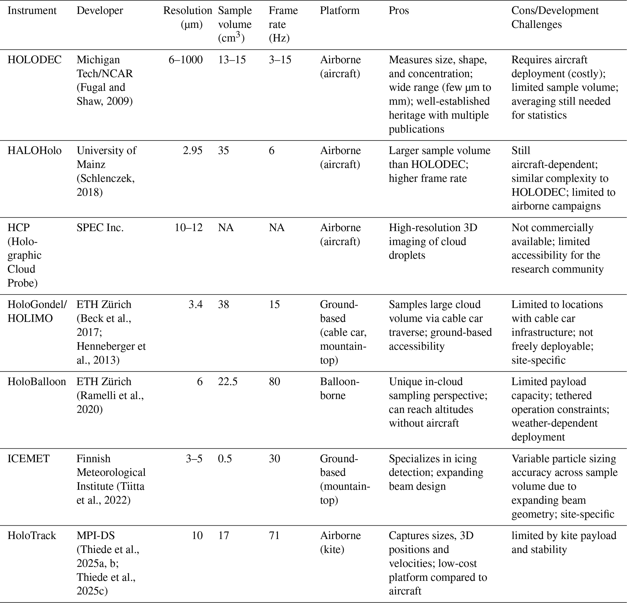
NA – not available.

1.2.2 Holographic techniques development/challenges

• 1.

  Designing a holographic instrument involves several choices that together determine overall system performance. A digital inline holographic system comprises two principal components: a camera imaging system and a coherent light source, typically a laser. The specific hardware selected and the geometry in which it is arranged directly affect holographic quality, and it is essential that the camera specifications be matched to the illumination properties. The key trade-offs are discussed in the following sections: Laser

  • –

    Wavelength: Laser wavelength affects the diffraction of particles and the fringe spacing. Smaller wavelength improves detectable spatial resolution of detected particles. This is why a UV laser is desirable. A visible (e.g. green) laser might also work, but if the same size particles should be detected, the optical magnification should be much larger.

  • –

    Mode: A pulsed laser is needed to minimize motion blur when recording holograms with a slow-framerate camera imaging fast-moving particles. The short pulse freezes the motion by illuminating the sample volume for only an instant, capturing the particle interference pattern in a single frame. This effectively produces a sharp snapshot of the particles.

    Alternatively, a continuous-wave (CW) laser can be used if paired with a high-framerate camera operating at very low exposure times. Without sufficiently short exposures, CW illumination leads to blurred images or streaks due to particle motion, which is an important limitation in high-speed flows or when observing fast-moving cloud droplets.

  • –

    Energy: The laser pulse energy must be sufficient to illuminate the full sample volume and produce detectable holographic fringes with an adequate signal-to-noise ratio. The entire camera should be illuminated without dark edges. It should be high enough to account for sample volume length, beam size, optical losses, particle properties, and detector sensitivity, but low enough to avoid camera saturation, excessive background scatter, or particle disturbance. Uniform illumination is also important to minimize spatial bias in particle detection.

• 2.

  Camera options with pros/cons

  • –

    Speed: As previously mentioned, the Camera frame rate should match the illumination source. When using a pulse laser source, the camera acquisition and laser trigger must be synchronized so that each frame records only one laser pulse. If multiple pulses occur during a single frame, fast-moving droplets may appear multiple times in the same hologram. If using CW illumination, then the camera exposure time should be short enough to keep particle displacement below the allowable motion-blur limit.

  • –

    Pixel size: The ideal pixel size is as small as possible, so small particles can be detected. The minimum size particle to be detected is two pixels in diameter; below that, it is too uncertain and could be noise (Henneberger et al., 2013; Kaikkonen et al., 2020). The pixel size and the number of pixels determine the overall size of the focal plane array, which in turn sets the achievable sample volume. This ultimately limits how large a sample volume can be used in practice.

  • –

    Detector size: Detector size should be as large as possible to capture a large sample volume.

  • –

    Frame rate: Frame rate is a trade-off: For particle tracking, a high-speed camera is necessary to capture the same particle many times in the same frame. However, these cannot run for hours, and even if they could, too much data that cannot be processed instantly would be recorded. So, we aim for two sets: one low-frame-rate camera that can record for many hours and gives us an idea of what the conditions in the chamber are, and a system with two high-speed cameras for particle tracking.

A holographic instrument is crucial for atmospheric research because it provides comprehensive and high-resolution measurements of cloud droplets, enabling a deeper understanding of cloud microphysics and dynamics.

As outlined above, holographic instruments such as HOLODEC, HALOHolo, HoloGondel, and others have demonstrated remarkable capability in simultaneously capturing the size, shape, three-dimensional position, and concentration of cloud droplets within a sample volume – a feat that conventional single-particle probes cannot achieve. Beyond these static microphysical properties, holography also offers the unique potential to track the movements of individual droplets across successive hologram frames, enabling direct observation of particle velocities, turbulence-driven relative motion, and even collision-coalescence events as they occur. However, this tracking capability comes at a higher cost: holographic reconstruction is a complex technique that requires sophisticated data analysis, and extracting full three-dimensional trajectories from dense hologram sequences demands substantial computational resources and processing time. This creates a fundamental tension – while holographic tracking can provide unparalleled microphysical detail, it is impractical to apply continuously over extended measurement periods or across large datasets.

1.3 Particle Image Velocimetry (PIV) and Particle Tracking Velocimetry (PTV) Methods

Particle Image Velocimetry (PIV) offers a complementary path forward. It is a widely used technique for measuring fluid flows (Willert and Gharib, 1991). Unlike Particle Tracking Velocimetry (PTV), PIV adopts a Eulerian approach, providing a macroscopic description of velocity at multiple points in space. This generates vector fields offering a detailed representation of the fluid flow over an area of interest. PIV is particularly robust in delivering dense, instantaneous velocity fields for a defined interrogation region and is well-suited for applications involving high particle concentrations.

On the other hand, PTV provides insights into individual particle movements, making it ideal for capturing complex dynamics, such as transient phenomena and rapid changes in flow behavior (Lu et al., 2008). In essence, PIV and PTV are complementary techniques for studying fluid flow dynamics: PIV offers an overarching view of particle flows, while PTV emphasizes individual particle trajectories.

Both Particle Tracking Velocimetry (PTV) and Particle Image Velocimetry (PIV) are highly suitable techniques for characterizing clouds, with cloud droplets serving as effective tracer particles. PTV specializes in tracking individual particles, measuring their velocities, and capturing droplet dynamics such as growth, ice crystal formation, aggregation, coalescence, and collision processes. On the other hand, PIV excels in providing flow characterization, assessing turbulence, spatial averaging, and identifying fluid currents, including phenomena such as evaporation and condensation.

In this study, we used a spray nozzle to evaluate the PIV setup. The spray nozzle generates inherently turbulent and chaotic fluid flows, and was aligned to direct particle motion primarily along the x-axis. This configuration facilitated testing of instantaneous velocity fields and enabled the determination of average velocity fields.

Because the event-based camera responds only to changes in pixel intensity, it captures fluid motion efficiently. Its low latency resolves fast-moving flows, while the sparse output reduces overall data bandwidth. The camera also operates at low power over a USB connection, which allows velocity fields to be displayed in real time during acquisition. The high speed camera used for HOLODROPS-TRACK requires up to 75 W and an external trigger to begin recording. Its high data rate means that frames are written to an onboard buffer, which must then be offloaded into a physical hard drive once acquisition is complete. HOLODROPS-TRACK is delayed further by the holographic reconstruction required before velocities can be recovered. Table S1 in the Supplement summarizes the resulting differences in power, data rate, and time to a usable velocity estimate.

The remainder of this paper is organized as follows. Section 2 describes the development of the new holographic system, including two operational configurations, with a particle-tracking mode complemented by an ePIV setup. Section 3 presents the calibration, characterization, and validation of all three configurations, covering laboratory calibration and initial testing as well as a field deployment in an outdoor drizzle case. Section 4 summarizes the main findings and offers an outlook on future developments and improvements.

2 Prototype Development and Instrument Description

2.1 HOLODROPS prototype

We developed two separate holographic configurations, HOLODROPS and HOLODROPS-TRACK. HOLODROPS is designed for long-term, high precision measurements of ongoing cloud conditions, while HOLODROPS-TRACK is meant to be operated in limited time frames to measure turbulence by tracking the individual particles in the sample volume. HOLODROPS uses a 31.4 megapixel machine vision camera (Prosilica GT6400, Sony IMX342), whereas HOLODROPS TRACK operates with an 8.3 megapixel camera (Kron Technologies, Chronos 4k12). In this paper, HOLODROPS is treated as the high resolution system, and it is referred to in that way throughout the text. In contrast, HOLODROPS TRACK employs a camera with lower resolution but much higher frame rates, making it the high speed counterpart to HOLODROPS.

Due to these two distinct purposes, the systems contain different components to maximize the benefits of each. The layout of both HOLODROPS and HOLODROPS-TRACK is the same, and the setup for HOLODROPS-TRACK is shown in Fig. 1. In both cases the hologram plane is collocated with the camera sensor. If they are separate, particles could be located between the camera and hologram plane, which would show up as particles in the sample volume due to the processing. This concern is removed in HOLODROPS.

HOLODROPS contains a UV-laser (355 nm) and a high-resolution camera (3.45 µm resolution), such that very small particles (>6.9 µm) can be imaged accurately. However, such a fine resolution limits the instrument's maximum output to 6 Hz. The frame rate is therefore constrained by the focal plane array readout bandwidth, digitization electronics, and data-transfer capacity rather than by the laser pulse duration. The current design of HOLODROPS uses an enclosure for all components, enabling safe laboratory operation. It is designed in a modular way so that the system can be adapted to a variety of laboratory situations, including varying the desired sample volume. While the enclosure itself is made of laser-safe materials, the optical path passes through uncoated calcium fluoride windows. With this design, the benefits of HOLODROPS become obvious; the variable sample volume that allows distances of several meters enables the use of HOLODROPS in many different laboratory settings, including cloud chambers, as well as a flexible setup on ground-based observatories. The sample volume for HOLODROPS at 1 m is approximately 3000 cm³.

HOLODROPS-TRACK contains a different high-speed camera with 4.5 µm resolution, combined with a continuous-wave (CW) green laser (532 nm). It is intended to be operated in short time bursts when particle tracking is desired due to the large data bandwidth produced by this camera operation. The highest data acquisition rate for this system is 1397 FPS at 8-bit. Additional information about the prototype system is included in Table S1.

Currently, this instrument can be deployed for brief periods of time outside. A waterproof version has been built and is under testing for long-term outdoor operation. For extended outside operations, we added temperature modulation unit (including heaters and cooling fans) to keep the components at desirable operating temperature. We also plan to add an algorithm for triggering HOLODROPS recording, i.e., only when there is a cloud or precipitation, in order to limit the amount of data collected that has no droplets. For an outdoor deployment, e.g., on a mountaintop, HOLODROPS also needs to be easily aligned between the camera and the laser, which we have achieved with an adjustable 3D-printed mount between them, designed to minimize its impact on airflow. Lastly, the instrument should always be pointed into the wind to reduce droplet shading and shattering/breaking of hydrometeors; as such, a wind vane would need to be added to the current design.

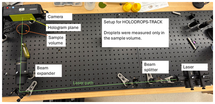
Figure 1 A prototype HOLODROPS, configuration for High-Speed Camera sampling, same setup used for High-Resolution sampling. The hologram plane is located at the camera sensor, without relaying optics.

2.2 ePIV prototype

Experimental Setup for PIV Using an Event Camera

Neuromorphic event cameras operate by monitoring changes in the intensity of light at each pixel asynchronously rather than recording full image frames at fixed intervals. Every pixel functions independently and continuously checks whether the brightness it receives changes beyond a preset contrast threshold. When a significant change occurs, that pixel produces a positive event, and when the brightness decreases it produces a negative event containing its location, the exact time of the change. Because the sensor reports only meaningful changes, it generates a sparse stream of data that represents motion in a scene with remarkable temporal precision. This approach removes motion blur, reduces redundant information, and provides excellent performance in situations with rapid movement and high dynamic range (Gallego et al., 2020).

The event camera-based PIV system (ePIV) employs a continuous green laser (wavelength: 532 nm) to illuminate water droplets. A cylindrical lens is used to focus the laser light into a thin line along the z-axis, forming a thin laser sheet to illuminate the particles. A camera is carefully positioned and focused on the laser sheet at a distance of approximately 50 mm. Water droplets for testing are introduced into the setup using a nebulizer (Fig. 2).

In this experiment, an event camera serves as the imaging sensor. Event cameras, also known as neuromorphic cameras, are inspired by the functioning of the human eye. Instead of capturing traditional intensity-based images, they operate asynchronously, measuring changes in pixel intensity. This distinctive readout results in low latency and sparse data representation, with latency as low as 100 µs. Though event cameras do not record frames in the conventional sense, an equivalent frame rate would be comparable to 10 000 FPS (Gallego et al., 2020). In contrast, traditional high-speed cameras face bandwidth limitations as they capture full frames at high framerates. Event cameras overcome this limitation by only measuring changes, dramatically reducing the amount of data captured per frame. Additional advantages of event cameras include their lightweight design and lower power consumption compared to high-speed cameras. The event camera uses 1.5 W of power while the high speed camera uses 75 W of power. The event camera is $\mathrm{30}\times \mathrm{30}\times \mathrm{36}$ mm in size compared to the high speed camera which is $\mathrm{188}\times \mathrm{111}\times \mathrm{53}$ mm. The vent camera is 32 times smaller than the high speed camera, and requires 50× less power to operate.

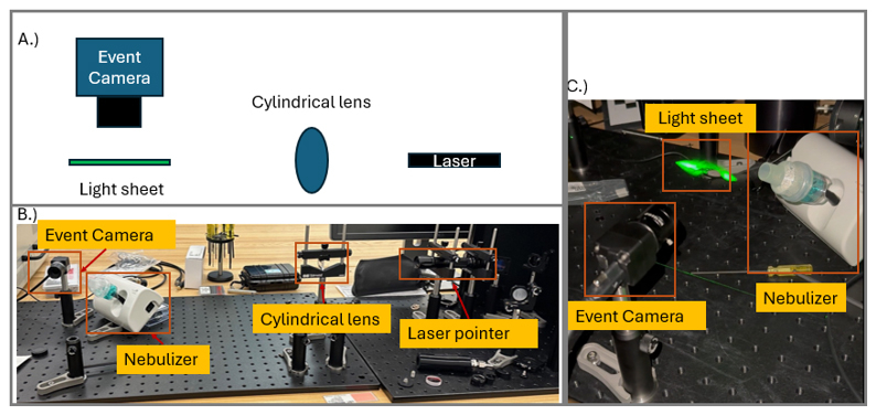
Figure 2 (A) Typical PIV set up. (B) Side view of the experimental setup. (C) Image of the water droplets illuminated by the laser.

Event cameras are highly effective at imaging fluid flows due to their ability to inherently measure changes in pixel intensity (Willert and Klinner, 2022). This characteristic allows for the automatic detection of particles within a frame, eliminating the need for manual thresholding and significantly streamlining the analysis process. Furthermore, the low latency of these cameras enables the detection of particles at high speeds, making them ideal for dynamic imaging applications.

Unlike standard cameras that capture entire frames, event cameras record only changes in pixel intensity, focusing solely on alterations within the scene. This approach minimizes redundant information and significantly reduces data bandwidth requirements. For instance, fluid flows captured from the nebulizer are efficiently visualized using this technique.

To facilitate analysis, the event data is transformed into pseudo-frames over fixed time intervals. This conversion ensures compatibility with open-source Particle Image Velocimetry (PIV) software (Shirinzad et al., 2023). In this study, the openPIV package was utilized, which applies cross-correlation methods within defined interrogation windows to calculate fluid velocity fields across different spatial regions (Willert and Gharib, 1991).

3 Calibration, Characterization and Validation

Calibration and characterization are very important to ensure accurate measurements in the future. Therefore, we measure the effective size of individual pixels of the system, its efficacy and accuracy in processing in a few different ways. These are done under controlled conditions in the laboratory, to determine the possibilities of the instrument in ideal conditions. First, we use a USAF1951 resolution target to determine the effective pixel size at various distances and to determine the best distances between camera and laser. Then, we use calibration glass beads of known sizes to confirm with more realistic shapes. Synthetic holograms were used to determine the accuracy of the particle detection and tracking methods. Lastly, we used a nebulizer to confirm how water droplets are seen and detected by the system.

3.1 Resolution target

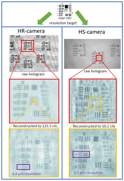
We used a USAF1951 resolution target in the sample volume of both systems to verify the effective pixel sizes. This target has patterns of three horizontal and vertical lines of various sizes, and the smallest completely resolvable pattern shows the resolution of the system (Fig. 3). The resolution of the HR camera system is as expected, with a 4.4 µm resolution at a distance of 125.5 cm. This means that features of 4.4 µm can be resolved at this large distance, and even more conservative approaches of twice the resolution will yield detectable droplets of 8.8 µm diameter, and therefore below 10 µm, which we aimed to achieve. The HS camera system was tested at a shorter distance since in real conditions it will also be closer to the objects to detect. It also performed really well, with a resolution of 5.5 µm; again, if twice this resolution is used, we can detect droplets at 11 µm, the size range we were aiming for.

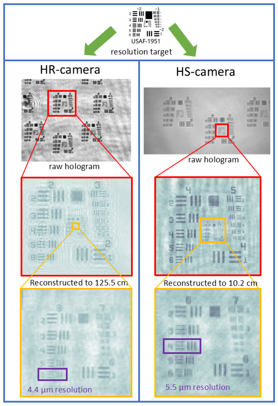
Figure 3 Resolution target results with both the high resolution (left column) and high speed (right column) camera.

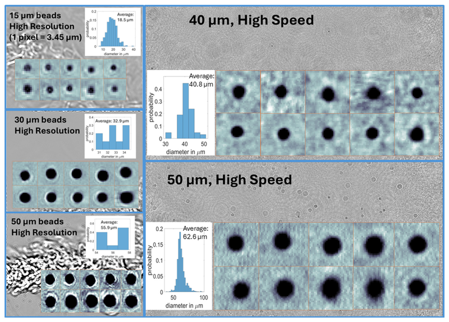
Figure 4 Results of glass bead tests with both systems: High resolution (left) and high speed (right) camera. Each panel shows a reconstructed plane of one of the holograms taken for this size (background), 10 examples of what beads looked like and the determined size distribution. The histogram plot x-axis is the diameter in µm and y-axis represents the probability density at each size bin.

3.2 Glass beads

To assess sizing accuracy for spherical targets across the droplet size range, dry borosilicate glass microspheres (Duke Standards) were introduced into the sample volume. The beads have NIST-traceable mean diameters of 14.4 ± 0.8, 29.5 ± 1.0, 42.3 ± 1.1, and 49.3 ± 1.4 µm, so the reference diameter is known to better than 3 % in all cases. As expected, the bead datasets are noisier than the droplet datasets, because residual dust from the atomizer,aerosol from the carrier flow and in general strong turbulence are visible in the example holograms in Fig. 4. Because the dry beads must be pneumatically introduced into the sample volume, the carrier jet introduces both particulate contamination and density gradients that act as a weak phase screen on the illuminating beam.

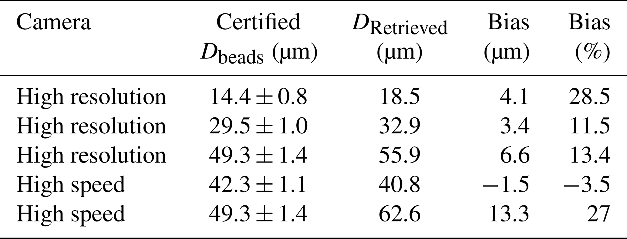
For the high resolution camera system (1 pixel =3.45 µm), the 14.4 (15), 29.5 (30) and 49.3 (50) µm batches were used; the smallest is resolved by roughly four pixels and therefore probes the lower limit of the retrievable size range. It detects all three sizes well, as shown in Fig. 4. All three batches were detected and sized within two pixels of their certified means (Fig. 4, left column): 18.5 µm for the 14.4 µm beads, 32.9 µm for the 29.5 µm beads and 55.9 µm for the 49.3 µm beads, corresponding to biases of +1.19, +0.99 and +1.91 px respectively. Although these correspond to relative errors ranging from 11 % to 29 %, the bias expressed in pixels is nearly constant and shows no systematic dependence on particle size. This is characteristic of a fixed edge-localization offset in the sizing algorithm rather than an error in magnification or reconstruction geometry, which would instead produce a constant relative error. The mean high-resolution bias of approximately +1.3 px sets the practical sizing accuracy of the system and, as expected, dominates the relative error budget at the smallest sizes.

The high speed system has a shorter exposure time, which increases the reliable retrieval limit. Thus, the 42.3 (40) and 49.3 (50) µm batches were used instead, consistent with the intended application of the high-speed configuration to the larger, faster-falling drizzle mode rather than to the small cloud droplet mode. The 49.3 µm batch was measured with both cameras and therefore provides a direct comparison in which the target is physically identical, and only the imaging chain differs.

While the 40 µm were detected very close to the actual size (40.8 µm from HOLODROPS), the 50 µm beads, by contrast, were retrieved at 62.6 µm, an overestimate of 13.3 µm or 27 %. Since the same bead batch was sized to 55.9 µm by the high-resolution system, and since the 42.3 µm beads measured with the same camera show no comparable bias, this discrepancy cannot be attributed to the reference material or to a fixed instrumental offset. Instead, the most likely explanation are the injection conditions: the heavier 50 µm beads required a stronger carrier flow to be entrained into the sample volume, thereby increasing both the interference aerosol loading and the inhomogeneity along the beam path. The same trend, though weaker, is present in the high-resolution data. The effect is amplified in the high-speed system because its shorter exposure time and larger pixels yield a lower signal-to-noise ratio per frame, so a given level of background fluctuation degrades fringe contrast and, hence, edge localization more severely. We therefore interpret the 49.3 µm high-speed result as an upper bound on the sizing bias under unfavorable imaging conditions rather than as an intrinsic property of the instrument. In practice, measurement uncertainty depends somewhat on conditions, as indicated by the high uncertainty encountered when a strong carrier flow is present. Therefore, we conclude that the uncertainty of size measurements by HOLODROPS is at least 1 pixel and at most the maximum bias we measured with beads, between 3.45–6.6 µm for the high-resolution camera and 4.5–13.3 µm for the high-speed camera. For most conditions with clean holograms, the bias is expected to be closer to the 1-pixel size, while with strong turbulence and noisy holograms it can be closer to the upper bounds.

Table 2 Glass beads information with the retrieved mean diameters.

3.3 Outdoor drizzle measurements

To test the instrument under realistic conditions, we deployed HOLODROPS at an instrument platform outside during a drizzle event on 13 March 2026 in Richland, WA, USA. The setup and results are shown in Fig. 5. The sample distance between the camera and laser system was 32.3 cm, leading to an effective sample volume of 106 cm³. Unfortunately, the system was not properly aligned, leading to the shading of parts of the hologram (large semi-circle in the right-hand part of the hologram in Fig. 5), which will necessitate some improvements to the setup. It reduced the sample volume by 12 %, still giving a very large sample volume for this experiment. The black covers shown in the setup were a necessary safety feature eliminating laser scattering, and while it will impact airflow and thus results, there are plans to improve laser safety and deploy to a location where these safeguards are not needed.

During the duration of the measurement was constant drizzle with varying intensity, shown in the time series in Fig. 5. The average size of drizzle drops was 377 µm, with a large spread. Despite all the challenges, the holograms are of great quality, and the drops are well detected, with clear images obtained from reconstruction.

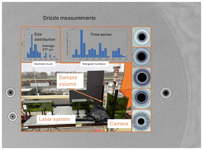
Figure 5 Results from outdoor drizzle measurements: Background shows an example of a hologram with three drizzle drops within the same frame; insert shows the size distribution and time series measured as well as the experimental setup and five examples of drizzle drops.

Overall, the outdoor deployment was a successful proof of concept, and HOLODROPS will be able to be used in both indoor and outdoor situations. For long-term outdoor operation, a few improvements will be made, such as temperature control of the electronics, waterproofing of the housing, better splash-resistance of the windows, and improved laser safety with less impact on the sample volume air-flow. We also saw some movement of the components in wind, and therefore a sturdier, smaller enclosure of the laser setup will be designed. However, even without these future improvements the system works remarkably well with clean data.

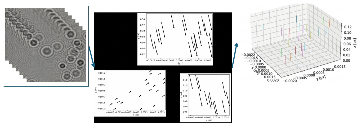
Figure 6 Results from particle tracking with synthetic holograms. Left: raw synthetic holograms. Center: Reconstructed particle movements in all three planes. Right: Particle tracks and movements in space.

3.4 Evaluation of Particle Tracking Capability of HOLODROPS-TRACK

With the use of high-speed cameras for image and hologram captures, we can capture droplet locations and sizes in rapid succession. This creates the possibility of employing particle tracking software to infer additional information from the droplets, such as individuals a combined particle velocities in 3D. This will require software that can link particles together between holograms and determine the vector velocities for further analysis. Now there is no particle tracking software specifically designed for droplet holograms, but there are many general particle-tracking software packages that could be valid candidates.

For this project, Holosuite (Schlenczek, 2018; Fugal et al., 2004) was used to reconstruct particles and determine their 3-dimensional positions between frames, and Trackpy was used to link particles across frames to represent the same particle. Along with information on the pixel sizes and frame rate of the camera, it allows us to determine the velocity and direction of each individual particle. We used synthetic holograms for testing of the tracking calculations, and the results are shown in Fig. 6. Each simulated particle is set to move 3 mm in z and 3 pixels, which, at 3.5 µm per pixel for this simulation, translates to 10.5 µm in both the x and y dimensions, and the results reflect that. Each particle was found and moved by the prescribed distance.

The nebulizer flow was imaged using the high-speed HOLODROPS-TRACK holographic system. Frames were recorded at 1397 frames per second with an exposure time of 15.99 µs. Raw holograms were reconstructed using the Holosuite software (Schlenczek, 2018) to obtain three-dimensional particle positions.

After reconstruction, particle trajectories were identified using the trackpy Python package (Allan et al., 2018; Crocker and Grier, 1996) Particle linking was performed with a search radius of 600 µm, and trajectories shorter than 4 frames were excluded from further analysis.

The positional uncertainty in the holographically reconstructed particle data is approximately one pixel in both the x and y directions, where each pixel corresponds to 4.5 µm in the camera plane. The uncertainty in the z direction is governed by the axial reconstruction step size, which is about 100 µm. Random error in particle trajectory positions is estimated by fitting a polynomial to each identified track and evaluating the residual variance and covariance of the fitted coefficients (Janke and Michaelis, 2021). This method does not provide absolute position accuracy, and particles that deviate from the fitted trajectory can add to the residuals. This method also does not capture systematic depth errors. The positional residual standard deviation is calculated using ${\mathit{\sigma }}_{\mathrm{p}}=\sqrt{\frac{\mathrm{\Sigma }j{\left(p_j-{\widehat{p}}_j\right)}^{\mathrm{2}}}{n-\mathrm{3}}}$ with σ_p as the position uncertainty, p_j is the measured particle position, $\widehat{p}$ is the fitted position, and n is the number of points in a track.

Velocity uncertainties are obtained by analytically differentiating the second-order polynomial fit to position as a function of time. For each coordinate, the trajectory is represented as $p\left(\mathit{\tau }\right)=a_{\mathrm{0}}+a_{\mathrm{1}}\mathit{\tau }+a_{\mathrm{2}}{\mathit{\tau }}^{\mathrm{2}}$, with $\mathit{\tau }=t-\stackrel{\mathrm{‾}}{t}$ as the center time. With differentiation this give $v\left(t\right)=a_{\mathrm{1}}+\mathrm{2}{a}_{\mathrm{2}}\mathit{\tau }$. The residual variance of the position fit is used to estimate the covariance matrix, $C=\frac{{\mathit{\sigma }}_{\mathrm{p}}^{\mathrm{2}}}{X^{T}X}$, with $\mathit{\beta }={\left[a_{\mathrm{0}}{a}_{\mathrm{1}}{a}_{\mathrm{2}}\right]}^T.$ The uncertainty in velocity is then propagated from the coefficient covariance matrix using the Jacobian J=[012τ], such that σ_v(t)²=JCJ^T. This approach accounts for both individual uncertainties in the fitted linear and quadratic coefficients and is applied to each measured velocity component (Janke and Michaelis, 2021).

A total of 392 particles were initially tracked, and trajectories containing fewer than four points were removed, leaving 157 usable tracks. Velocities were then evaluated at each time step from the differentiated polynomial fits. Table 3 in the manuscript summarizes the RMS positional uncertainties and mean velocity uncertainties.

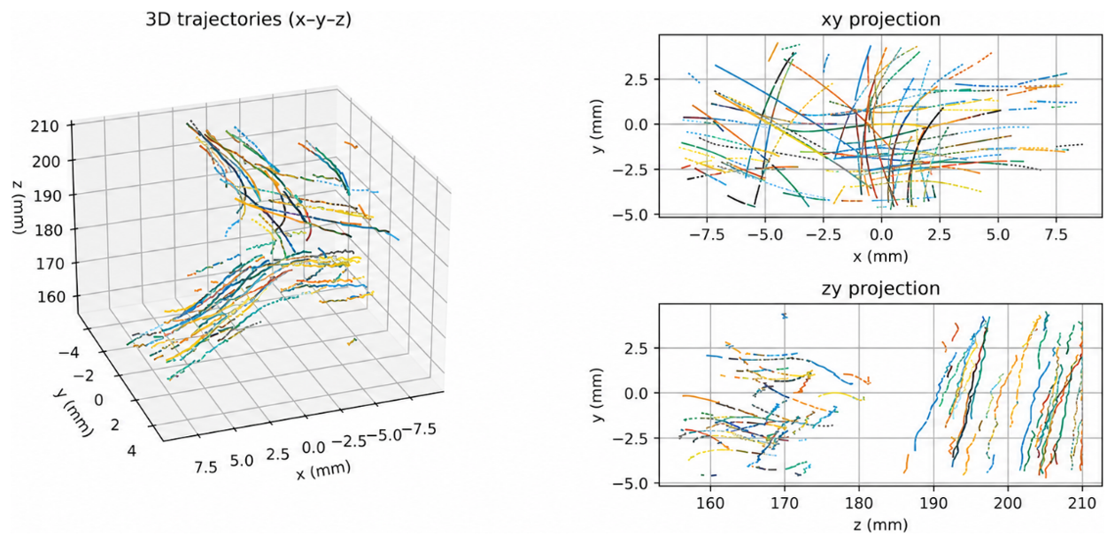
Figure 7 Left: Three-dimensional particle trajectories obtained from holographic reconstruction, along with their 2D projections. Right Top: x–y projection of the particle tracks. Each color represents a different particle. Left Bottom: z–y projection of the particle tracks.

Table 3 Mean uncertainty values for the positional and velocity components for the tracked particles.

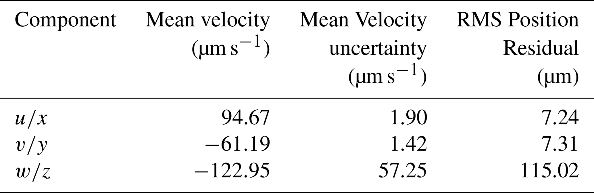
Figure 7 presents representative particle trajectories reconstructed from the holograms. Each color denotes a distinct particle track. The three-dimensional paths are shown alongside their two-dimensional projections onto the x–y and y–z planes. The left panel displays the y–z projection, while the right panel shows the x–y projection.

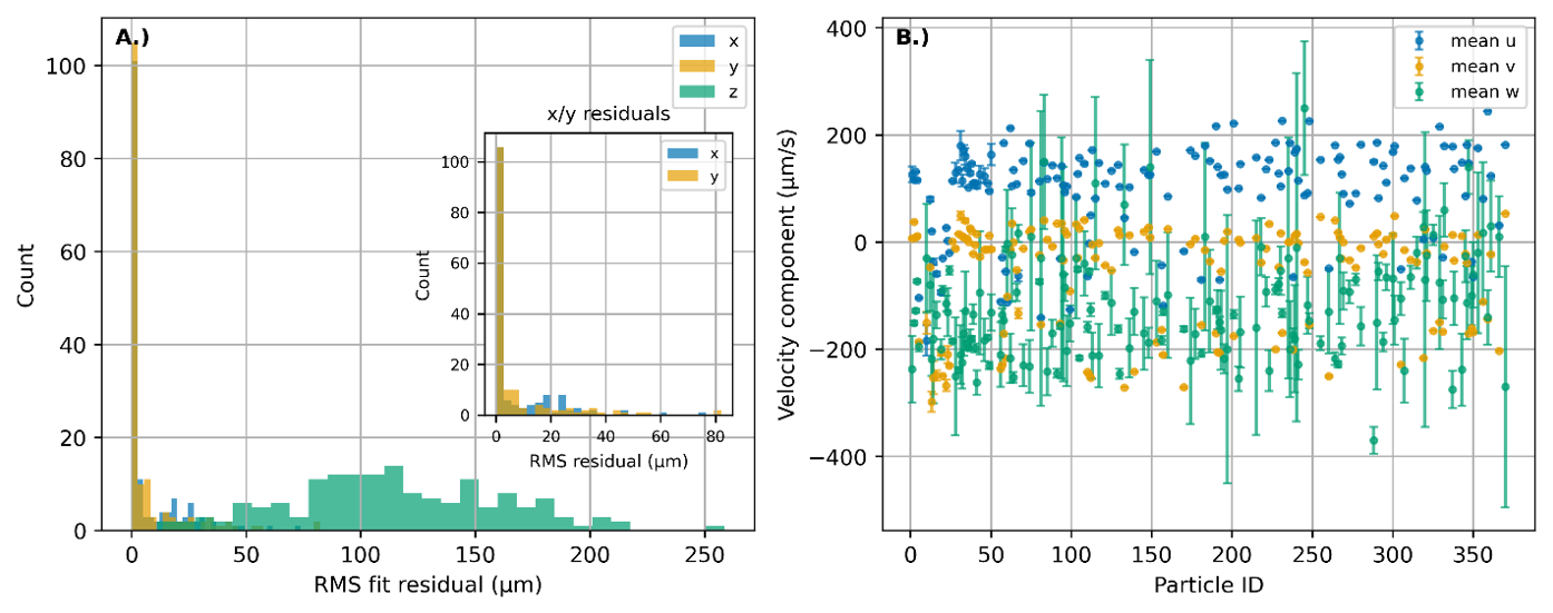
Figure 8 (A) displays the residual distributions for the particle-track positions obtained from the polynomial fits, with the inset highlighting the x- and y-component residuals. Panel (B) shows the velocity components and their associated uncertainties for each particle track. In total, 392 particle tracks were initially identified. After removing tracks shorter than 4 points, 157 complete particle trajectories remained for analysis.

Additional plots of RMS residuals illustrate the uncertainty distribution for each spatial component in Fig. 8. As expected, the x and y components exhibit smaller uncertainties because they are directly tied to pixel resolution, while the z component shows significantly larger variability due to its dependence on the axial reconstruction step. The residual distributions were found to be at x-position (7.24 ± 13.58 µm), y-position (7.31 ± 15.68 µm), and z-position (115.02 ± 53.10 µm).

These results confirm that lateral positional uncertainties are much tighter than axial uncertainties, consistent with the characteristics of digital in-line holography.

3.5 Evaluation of the Tracking Capability of ePIV

Establishing ground truth data for PIV can be difficult since fluid motion can be fast and complex. To assess the performance and uncertainty of the ePIV system, we generated synthetic particle-image data with known displacement fields. This provides ground truth data for quantifying position and velocity errors and follows established best practices for PIV uncertainty analysis (Sciacchitano, 2019). This approach will determine the displacement error for corresponding peak-to-peak signal to noise ratios (SNR) found with cross correlation. The goal is not to establish the absolute measurement uncertainty but rather to determine a practical displacement uncertainty estimates under conditions matched to our experiment. For this analysis, gray-scaled particle will be generated using Synthpix a PIV image generator (Terpin et al., 2026). This analysis does not take into account event sensor characteristics such as contrast threshold, polarity, and accumulation duration. Such effects could be simulated by using event camera simulators such as v2e, ESIM and others (Hu et al., 2021; Rebecq et al., 2018). Since the processing uses only on events and excludes off events, polarity is expected to have little effect on the uncertainty. How the contrast threshold affects the uncertainty is unknown, but because the scattered light from the particles appears bright compared to the background, as shown in Fig. 2C, it is suspected to have a minimal impact. The timing uncertainty is also expected to have a small effect, since the sensor latency is 100 µs and the smallest time interval is 1 ms, which is an order of magnitude larger. Accumulation time does influence the determined velocity fields and the uncertainty. However, for this analysis, the goal is only to demonstrate the feasibility by matching the experimental results. A rigorous study of parameters and inclusion of simulated sensor characteristics is planned for future work. The grey-scale simulated images should serve as a baseline for the estimated displacement uncertainty.

3.5.1 Synthetic Data Generation and Experimental Matching

We first established frame-based experimental statistics to ensure the simulations closely matched real measurements. Since the plume produced by the nebulizer only overlapped part of the imaging area, particle density was only calculated for interrogation windows with particles present. Particle density was calculated using a connected-component algorithm, and the pixel area of non empty interrogation windows. This allows estimation of the number of particles perpixel. Additional statistics, including particle diameter, intensity distribution, and active pixel area, were derived from autocorrelation analysis of experimental frames. These metrics provide realistic seeding conditions and ensure similar characteristics between synthetic and experimental data. This analysis was conducted for different time intervals from 1.0 to 10 ms, and showed comparable statistics across frames.

To simulate realistic PIV input, SynthPix was used to generate uniform displacement fields ranging from 1 to 9.5 px at randomized orientations, with 20 realizations per displacement magnitude (Terpin et al., 2026). The frame size (256 × 256) is sufficient for capturing statistical behavior without requiring full-frame simulations. Each synthetic pair was padded to accommodate edge displacements, ensuring physically valid particle origins.

A median filter was used to suppress isolated sensor noise in experimental data; however, because synthetic noise was not simulated, filtering was omitted in the synthetic pipeline.

The statistical parameters used to align the simulations with the experimental data included a seeding density of 1–3 particles per pixel, particle diameters ranging from 1.6 to 1.87 pixels with a variance of 0.3 pixels, signal-to-noise ratios between 1 and 1.2, total displacement magnitudes from 1 to 9.5 pixels, and 20 simulation realizations.

3.5.2 Velocity Field Computation and Uncertainty Estimation

Pseudo-frames were constructed at 1 ms intervals to align with the temporal resolution used during ePIV acquisition. These frames were processed using openPIV, employing cross-correlation within 16-pixel interrogation windows and a 19-pixel search area. Prior to processing, median filtering was applied to remove pixel-level noise inherent to the event camera. In addition, “off” events were removed from the images, and only “on” events were processed using openPIV. This simplifies the analysis since “off” events show the previous location of particles. Focusing on “on” events between pseudo frames clearly captures the gradual motion path between frames.

Velocity fields were calculated for each frame pair, and a time-averaged velocity field was formed by averaging all instantaneous velocity components across the full acquisition period. Though instantaneous velocities can be high, variations in droplet appearance within the light sheet lead to relatively small mean values.

Uncertainty quantification follows the established approach of comparing known synthetic displacements to measured correlation-based displacements. By matching simulation parameters – particle size, seeding density, intensity, and signal-to-noise ratios – to experimental statistics, the resulting displacement-error curves provide a consistent estimate on measurement displacement uncertainty only (Sciacchitano, 2019). Synthetic images do not take into account how the event cameras effects, such as contrast threshold, frame accumulation, and polarity. Coupling both processes is considered as a future effort.

Figure 9 shows the error for displacement vectors. The error is binned with respect to the peak-to-peak SNR to determine a corresponds to the experiment. The displacement error average values was found to be between 7.0–1.13 pixels and for a peak-to-peak SNR of 1 to 2.5. The vectors are transversed in random directions, so the errors for the x and y directions follow the same profile, and magnitude.

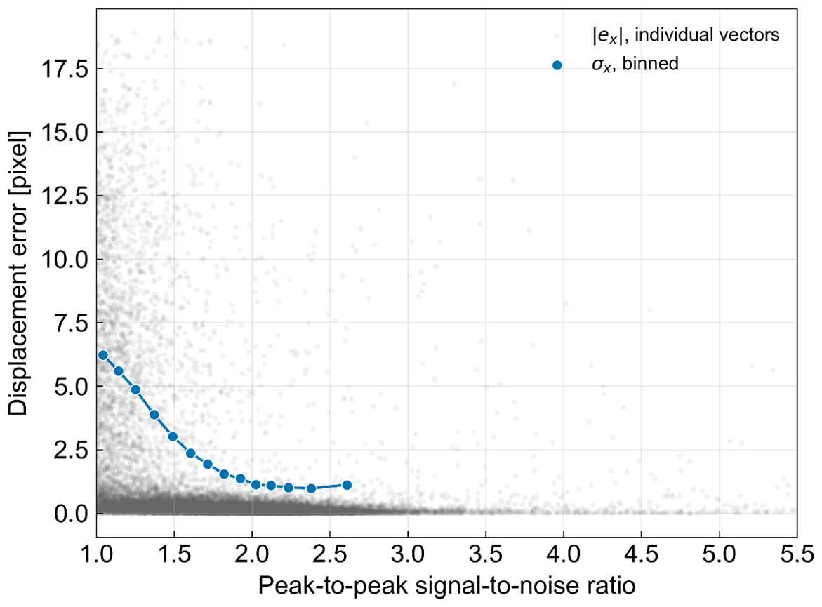
Figure 9 After calculating the error in displacement of simulated particles. The displacement error is binned with respect to the peak-to-peak SNR ratio. As the SNR increase the displacement error decreases providing an estimate for the particle displacement uncertainty from the determined SNR ratios.

After determining the displacement error, the error in the calculated instantaneous velocity or one velocity measurement can be determined from ${\mathit{\sigma }}_v=\frac{{\mathit{\sigma }}_{\mathrm{p}x}S}{\mathrm{\Delta }t}$ with σ_v as the velocity uncertainty, σ_px as the displacement uncertainty, S as the scaling factor, and Δt as the time interval. For our experiment, at 1 ms and a scaling factor of 0.033 mm per pixel makes the instantaneous velocity uncertainty σ_v=0.033σ_px with units of [mm ms⁻¹]. At the lowest SNR there can be 7 px error which works out to be 23.1 µm ms⁻¹, and at the highest SNR we can expect 1 px or 3.3 µm ms⁻¹ error. For longer duration measurements, the velocities are temporally averaged for frames that have particles present. Assuming the errors are independent, and the time uncertainties and scale uncertainties are much less than the random displacement uncertainties then the time average becomes $\stackrel{\mathrm{‾}}{{\mathit{\sigma }}_{\mathrm{v}}}=\frac{{\mathit{\sigma }}_{\mathrm{v}}}{\sqrt{N}}$ where N is the number of measurements (Sciacchitano and Wieneke, 2016).

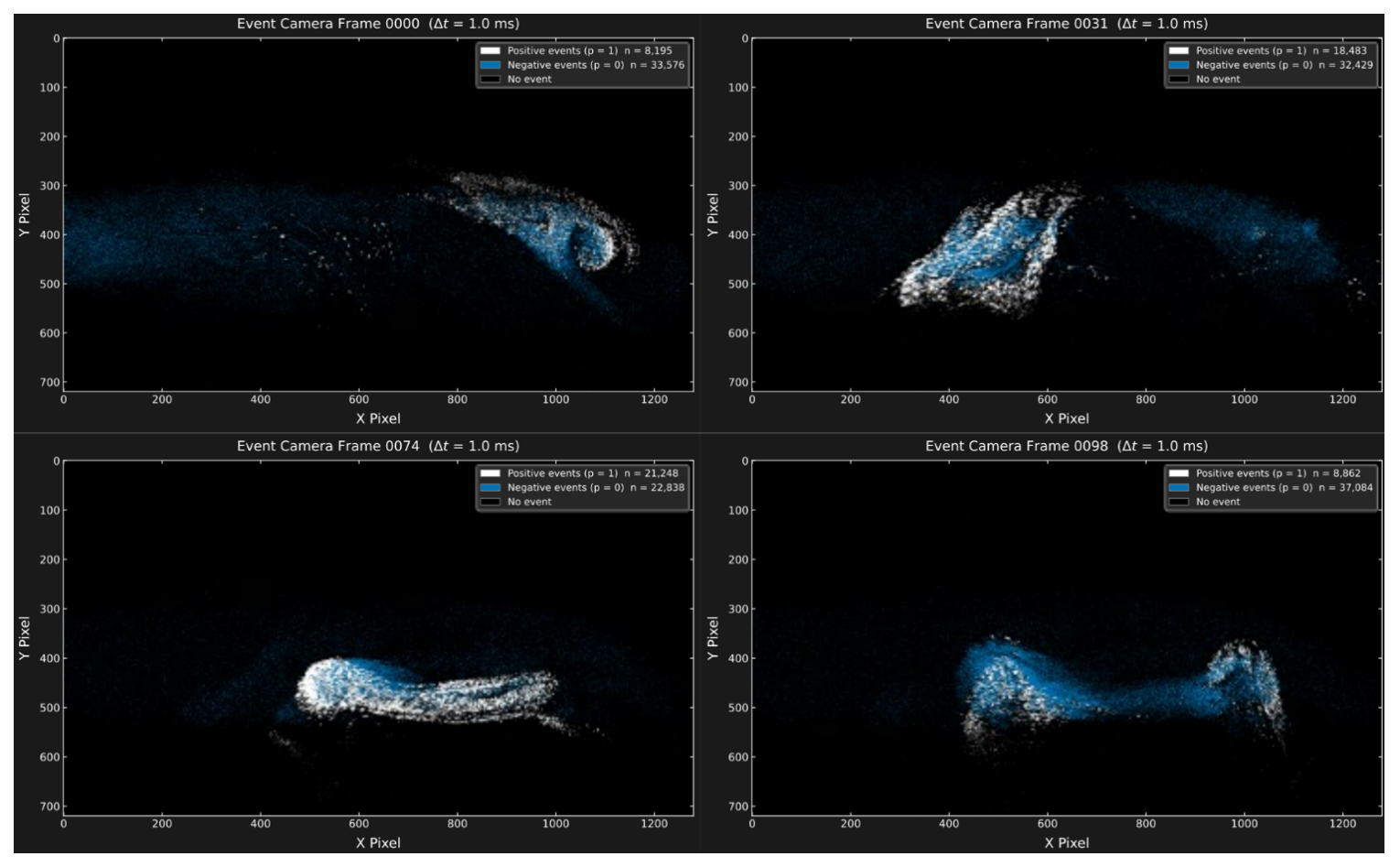
Figure 10 Captured fluid flows using an event camera: The event data was collected over a 1 ms time interval. Positive events, represented by white markings, signify areas where light intensity increases, while negative events, marked in blue, denote regions where light intensity decreases. These visualizations can be interpreted as follows: the white markings highlight the current locations of water droplets, whereas the blue markings indicate past positions of the droplets as they moved.

3.5.3 Orientation-Dependent Measurement Strategy

Since ePIV captures only two velocity components within a thin laser sheet, we collected measurements from two orientations to approximate broader flow characteristics: side-view (droplets traverse perpendicular to the laser-sheet propagation) and Front-view (droplets move within the plane of the sheet).

Each experiment used a 10 s acquisition period with 1.0 ms frame separations. Although many frames contain few particles, this duration is sufficient to resolve persistent background flow patterns and intermittent turbulent structures. Figure 10 shows the fluid flow of the particles captured using the event camera. Positive (white) events indicate increases in pixel intensity – corresponding to current droplet locations – while negative (blue) events indicate decreases in pixel intensity, tracing particle histories. These signatures provide intuitive visualization of flow direction.

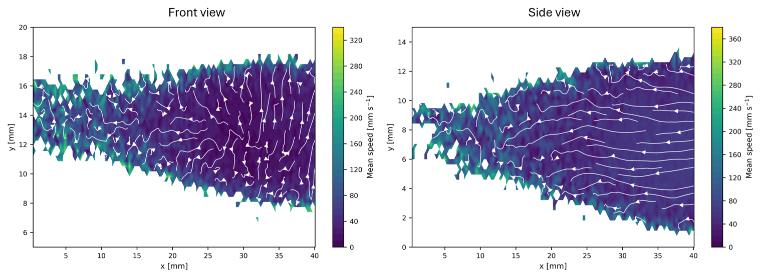
Figure 11 Time-averaged velocity fields measured using the ePIV system. Left: side-view measurement of the nebulizer relative to the light sheet. Right: front-view measurement. Arrows indicate the direction and magnitude of the measured velocity.

Spatial calibration was achieved using a checkerboard target placed 50 mm from the optical system. The resulting scale factor of 31.6 pixels per mm was applied to convert all measured velocities from pixels/s to physical units (mm s⁻¹). Instantaneous velocities occasionally reached 300 mm s⁻¹, though time-averaged values were closer to 20 mm s⁻¹. The full distribution of measured speeds is shown in Fig. 11.

3.5.4 Summary of ePIV Tracking Performance

Overall, the ePIV system effectively captures fluid motion using event-camera data. Synthetic-data matching ensures reliable uncertainty bounds, and dual-orientation experiments improve interpretation of complex flow structures. While ePIV measures only in-plane velocities, it provides rapid, low-latency flow information across many particles, making it strongly complementary to the holographic particle-tracking system, which resolves full 3D trajectories over shorter intervals.

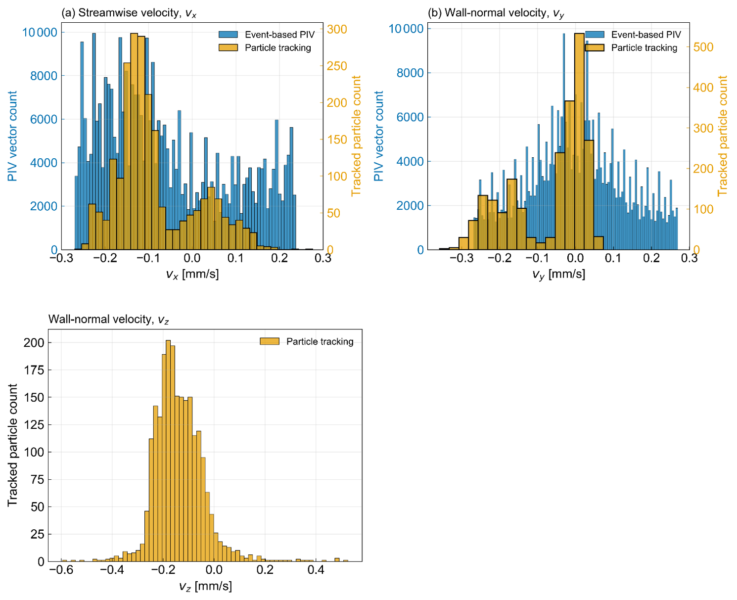
Figure 12 Comparison of velocity distributions measured by holographic particle tracking and the ePIV system. Top: front-view configuration, showing x-velocity (left) and y-velocity (right) distributions for both methods. Bottom: side-view ePIV measurements of the nebulizer flow field.

3.6 HOLODROPS-TRACK and ePIV Performance Comparison

The distributions of particle velocities are shown in Fig. 12. Both the ePIV measurements and the particle tracking results exhibit a pronounced mean flow in the negative x-direction. The distributions of the y-velocity components are approximately centered around zero for both methods, indicating no significant net motion in the y-direction. The laboratory environment has an HVAC system that continuously filters air. This system creates a steady draft in the laboratory and causes the particles to gradually flow in the x-direction, which was observed with both experiments. In the ePIV configuration, only a thin slice of the flow intersecting the light sheet is captured, so the measured velocities represent a cross-section of the full three-dimensional motion. In contrast, the HOLODROPS-HS holographic system resolves the full 3D position of individual particles over time, enabling direct estimation of all three velocity components, including the z-component. From the reconstructed z-positions, a net flow in the negative z-direction is observed. However, because the axial (z) position is inferred from holographic reconstruction, its spatial resolution is lower than that of the x and y coordinates, leading to comparatively higher uncertainty in the z-velocity component. Additionally, the ePIV measurements cover a longer time interval and a larger number of particles passing through the light sheet compared to the holographic particle tracking, which is limited to a shorter acquisition duration. As a result, the ePIV system is more sensitive to intermittent and turbulent fluctuations over extended.

In summary, this study highlights the effectiveness of event cameras and inline holographic imaging for analyzing fluid flows and particle scattering dynamics. The event camera's low latency and inherent ability to detect pixel intensity changes enabled the real-time visualization of velocity fields and particle distribution.

The HOLODROPS-TRACK system is bottlenecked by the need to save frames to the camera's onboard frame buffer. At full resolution and frame rate, the camera can only record about 11 s of data before filling its 128 GB memory buffer. After recording, the frames must be compressed and written to a storage device – a process that can take several minutes depending on the transfer method (SSD, Ethernet, or memory card). Recording 11 s at the maximum frame rate of 1397 fps produces roughly 15 000 frames, which require substantial processing time.

In contrast, the ePIV system reduces initial data volume due to its dynamic readout. Additionally, PIV using light-sheet illumination provides a high-contrast scattering signal that is much easier to detect than holographic images.

A particle-presence detector is an inexpensive, self-contained tool that can confirm whether particles are present. This type of sensor can be used to decide when to record images – over periods ranging from seconds to minutes – and offers a simpler and valid alternative to ePIV. However, particle counters measure concentration only within their sampling volume, and their inlet flow can disturb the sampled region. As a result, the sampling volume of the particle counter may not match that of the holographic system.

By comparison, ePIV provides an instantaneous event rate that can serve as a proxy for droplet number within the illuminated light sheet. It also provides velocity magnitude and direction, velocity-fluctuation intensities, vorticity, and distinctions between steady-state and transient flows. This information is valuable for determining where to deploy HOLODROPS-TRACK to image actual particles, measure particle sizes, track particle motion, and ultimately observe collision–coalescence in a dynamic environment.

As particle density increases, ePIV becomes less practical because it produces very large data volumes. Instead of scaling with frame rate and resolution, the sensor output scales with scene activity and dynamics. At high particle densities, data rates can reach up to 10 Gb s⁻¹, potentially causing readout saturation in the camera.

In the current experiment the two instruments were operated separately, although simultaneous operation is a goal for future deployments. In this configuration each sensor would use its own continuous wave laser. With two independent lasers the sources are mutually incoherent, and because the optical frequency difference is much greater than the exposure time, any interference averages to zero and the intensities simply add. As a result illumination from the ePIV system would appear only as an added background in the holographic measurement, which can be reduced by lowering the ePIV laser intensity. Cross talk can also occur in the other direction, since particles moving through the holographic illumination volume may appear in the event camera and produce particle flow over a larger depth range. Although the event camera can detect these particles, estimating depth from a single camera can be difficult, which is why a light sheet illumination was used in this work to define a measurement plane and restrict particle imaging to a narrow region.

Further reduction of cross talk can be achieved through spectral or geometric separation. For spectral isolation each system would operate at a different wavelength. Because holographic resolution depends strongly on wavelength, the holography system benefits from using the shortest available wavelength, while ePIV can operate at a longer wavelength such as 632 nm. Bandpass filters on each camera would then isolate the correct wavelength. Geometrically, the ePIV sheet can be placed upstream of the holographic volume and oriented perpendicular to the holographic optical axis so that it remains outside the field of view of the holographic sensor.

4 Conclusions and Future Work

Three new cloud measurement systems were developed: HOLODROPS, HOLODROPS-TRACK and ePIV and all were successfully characterized. The holographic systems are for long-term measurements of cloud droplet size distributions (HOLODROPS) and for short-interval particle tracking (HOLODROPS-TRACK). We successfully measured droplets larger than 8.8 µm in diameter, both in a laboratory setting and in a drizzle case outdoors. HOLODROPS-TRACK identified 3-dimensional tracks of particles moving through the sample volume, enabling direct studies of atmospheric turbulence and the detection of collision-coalescence in real time. HOLODROPS is designed to capture the full size distribution of cloud droplets up to drizzle and ice crystals, without the need for multiple instruments with narrow size ranges. HOLODROPS can run outdoors in drizzle; however, for longer deployments, the system still needs to be thoroughly weatherproofed. This is the next step for HOLODROPS, with the addition of waterproof housing. Furthermore, in the future HOLODROPS will be run in extremely hot and cold conditions, such as mountaintops in winter as well as the heat of summer, so heating and cooling elements for the critical electronic components (laser, camera and data acquisition) will be necessary.

Initial data processing for HOLODROPS and HOLODROPS-TRACK is currently done with Holosuite software, and is very time-consuming and computationally expensive. Ongoing work therefore focuses on reducing processing time with advanced machine learning algorithms, which would enable faster data access, and improving particle detection, leading to better data quality.

The ePIV is an event-camera based particle imaging velocimetry system, which perfectly complements the holographic measurements. It measures the flow directly and can be viewed in real time to inform ongoing measurements. Due to the dynamic readout, the ePIV system produces lower data volume and processing time, which is a limitation for the HOLODROPS-TRACK system. ePIV can operate continuously for long periods; it can inform users about cloud conditions much faster than holography and indicate when conditions would be ideal for collecting data with HOLODROPS-TRACK for finer detail. Both HOLODROPS-TRACK and ePIV can capture comparable fluid flows. Though the HOLODROPS-TRACK provides more detailed information on the individual particles tracked. In comparison, ePIV is not limited to individual particles and can gather information on a larger sample size. Future work will extend ePIV to measure 3-dimensional fluid flows.