Potential of point source imaging satellite instruments to infer diffuse methane emissions: a theoretical case study of the Near-Infrared Multispectral Camera (NIMCAM)

Satellite measurements have revolutionized methane monitoring, yet persistent clouds and aerosols often limit global-survey instruments like TROPOMI in the tropics. This study evaluates the potential of the Near Infrared Multispectral Camera for Atmospheric Methane (NIMCAM), a high-resolution instrument (60 m pixels) designed for point sources, to quantify large-scale diffuse emissions across tropical Africa. Through Observing System Simulation Experiments (OSSEs), we compare an in-orbit demonstrator and small NIMCAM constellations (3 and 5 satellites) against synthetic data from the TROPOMI (TROPOspheric Monitoring Instrument) instrument. Using Sentinel-2 cloud probabilities and downscaled MODIS aerosol optical depth products, we find that NIMCAM's finer spatial resolution significantly increases clear-sky data yields. A 5-satellite constellation provides up to six times more clear-sky observations than TROPOMI. As masking criteria for clouds and aerosols become more stringent, the ratio of NIMCAM to TROPOMI random error (${\mathit{\sigma }}_{\text{NIM}}/{\mathit{\sigma }}_{\text{TROP}}$) decreases. This occurs because TROPOMI's coarser footprint leads to a more rapid loss of data under strict thresholds. Using the GEOS-Chem chemical transport model and an ensemble Kalman Filter, we demonstrate that NIMCAM observations offer substantial added value in resolving tropical emissions. NIMCAM achieves higher uncertainty reduction than TROPOMI, particularly in regions and seasons where cloud and aerosol loading restrict coarser instruments. Our findings support using high-resolution methane technology to complement global surveys in monitoring diffuse tropical emissions.

1 Introduction

Over the last decade, the atmospheric growth rate of methane has surged to record levels (Feng et al., 2022, 2023, 2026; Pendergrass et al., 2025; Ciais et al., 2026), challenging existing climate projections. This acceleration is driven by two poorly understood variables: a massive spike in natural tropical emissions and potential large-scale but unresolved changes in the hydroxyl radical, the primary loss of atmospheric methane (Turner et al., 2019; Zhang et al., 2023; Feng et al., 2023). Other lines of evidence indicate that rising anthropogenic emissions – including fossil fuel combustion, agriculture, and waste – have also contributed to the recent methane increase, although their magnitude relative to natural source variability and changes in the atmospheric sink remains uncertain and actively debated in the literature (Skeie et al., 2023; Saunois et al., 2025).

The uncertainty surrounding these drivers is compounded by significant logistical and political barriers that now hinder the maintenance of ground-based monitoring networks in critical regions. Consequently, satellite-based remote sensing has become the backbone of methane research. Without space-borne observations, our ability to track shifting emissions across tropical wetlands and rapidly thawing high-latitude ecosystems would be virtually non-existent, leaving a dangerous blind spot in the global climate strategy. Since 2010, the two workhorses responsible for helping to monitor changes in atmospheric methane are the Japanese Greenhouse gases Observing SATellite (GOSAT) and the European TROPOspheric Monitoring Instrument (TROPOMI). However, the data from these instruments have spatial resolutions of several kilometres so that persistent clouds during wet seasons and elevated aerosol loading during dry season burning significantly reduces the number of clear-sky scenes (Qu et al., 2021; Balasus et al., 2023).

Meanwhile, there has been a rapid expansion of satellite instruments that have been designed, or have been repurposed, to observe small-scale point sources of methane, taking advantage of the sensitivity of methane in the shortwave infrared (SWIR) bands (Varon et al., 2021; Gorroño et al., 2023; Jervis et al., 2021; Mostafa and Du, 2025). Data from this class of instrument typically have spatial resolutions of tens of metres, so there is a higher probability of collecting data between clouds (Charuvil Asokan et al., 2025) and between regions of elevated aerosol loading. Recent work has shown that this type of data can influence emission estimates for both anthropogenic and natural emissions (Campbell et al., 2026). In this study we argue that while these newer instruments are less sensitive to methane, commensurate with diffuse sources of methane, the spatial resolution of their data and the co-addition of individual measurements can outperform the global survey instruments. We illustrate this using the Near Infrared Multispectral Camera for Atmospheric Methane (NIMCAM) mission concept, which has been designed specifically to locate and quantify emissions from large point sources. For the purposes of our experiment, we consider an in-orbit demonstrator (IOD) and constellations that range from three to five NIMCAM instruments.

Our study is focused on tropical Africa. The region hosts extensive wetland systems that are seasonally dynamic and poorly monitored and is also undergoing rapid land-use change and population growth, potentially contributing to increasing anthropogenic methane sources (Bullock et al., 2021; Zhang et al., 2021). Studies have shown that large-scale methane emission increases in this region can be attributed to changes in rainfall and subsequent wetland inundation (Lunt et al., 2019, 2021; Feng et al., 2022, 2023; Hardy et al., 2023). These studies have relied substantially on clear-sky data collected immediately downwind of emitting regions because of extensive cloud cover and biomass burning aerosol overhead of the emitting regions. This challenge is widespread across the humid tropics; Frankenberg et al. (2024) report very low satellite data yields due to persistent shallow cumulus clouds, with success rates of just 0.1 %–1.0 % in the Amazon during the wet season. They further show that increasing spatial resolution to 200 m could improve yields by two to three orders of magnitude, highlighting the importance of high-resolution observations for tropical greenhouse gas monitoring.

First, we evaluate the frequency and distribution of clear-sky data over tropical Africa for TROPOMI, the NIMCAM IOD, and a constellation of NIMCAM instruments, using high-resolution Sentinel-2 cloud probability data and downscaled MODIS aerosol optical depth data. We translate this information into gridded uncertainty estimates by co-adding data, assuming per-measurement random error estimates. Finally, using the GEOS-Chem model and an ensemble Kalman Filter (Feng et al., 2009), we use this information as the basis for OSSEs to evaluate the ability of NIMCAM to quantify large-scale diffuse emissions of methane over tropical Africa, predominately originating from wetlands, and compare it against synthetic TROPOMI data that has observed the same scenes. We focus on the months corresponding to the short rains (March and April) and long rains (October and November) seasons over the region in 2019 for which previous studies revealed substantial methane pulses (Lunt et al., 2019, 2021; Shaw et al., 2022).

In the next section, we describe the data and methods we use to evaluate the ability of NIMCAM data and compare its performance against synthetic TROPOMI data. In Sect. 3, we report our results for the clear-sky data distribution, co-addition of errors, and the corresponding methane emission estimates. We conclude the study in Sect. 4.

2 Data and methods

2.1 The Near Infrared Multispectral Camera for Atmospheric Methane

NIMCAM is a new EO satellite mission concept that has been designed to address the science requirements associated with identifying and monitoring changes in atmospheric methane due to emissions from large point sources. It has been under development at the University of Edinburgh since 2017.

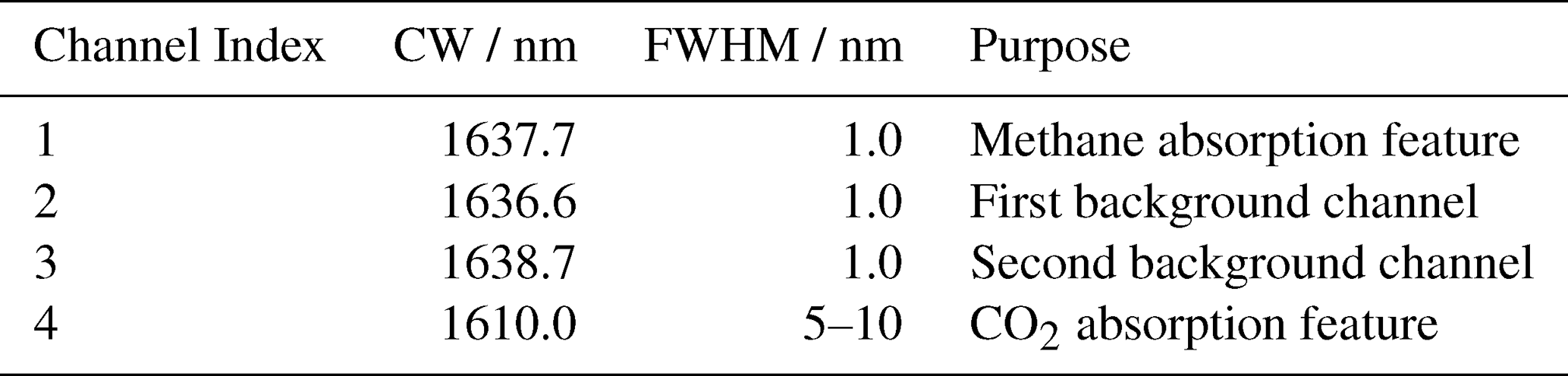
The core NIMCAM instrument is a multispectral imager, optimised for detecting changes in atmospheric methane at high spatial resolution and with global coverage. NIMCAM employs a novel design using a minimal number of spectral channels located near 1640 nm. Each channel features a very narrow bandpass width of 1.0 nm Full Width Half Maximum, with the channels positioned in close proximity to one another. The spectral design consists of an “on-band” channel located at a methane absorption feature, bracketed by two “off-band” channels which provide a fit for background spectral variations and other confounding species, as well as a fourth channel specifically for targeting CO₂ absorption. The channel specifications are shown in Table 1.

Table 1 Specifications for NIMCAM spectral channels detailing Central Wavelength (CW) and Full Width at Half Maximum (FWHM) for each channel.

The NIMCAM retrieval algorithm combines the Beer–Lambert law with a linear fit to the background spectrum to retrieve methane slant column density. Modelling work based on this three-channel design has demonstrated good methane signal contrast and reliable rejection of confounding water and ground reflectance signals. Observing in the near infrared brings several benefits including a greater sensitivity to near-surface methane compared with thermal infrared observations and reduced requirements for detector and optical system cooling. Narrow bandpass interference filters define the spectral channels, manufactured by depositing thin layers of coatings over a substrate material. Further details of the spectral design and methane retrieval algorithm can be found in Appendix A.

Other aspects of the NIMCAM flight instrument design include a telescope with primary aperture of 135 mm, imaging a cross-track field of view of 2.9°. We use a commercial Indium Gallium Arsenide (InGaAs) detector from Raptor Photonic, which provides a resolution of 640×512 pixels. Manufacturer-provided detector specifications have been used during our modelling work to assess the Signal to Noise Ratio of the system. NIMCAM operates with a swath width of approximately 30 km, and 60 m ground pixels. The narrow bandpass filters are arranged in strips across the field of view. As the scene moves under the instrument it sweeps across the filters, meaning a point on the ground is imaged through all channels during an overflight, providing the required channels of spectral data for each spatial pixel. Telecentric relay elements provide the necessary optical conditions to maintain filter spectral performance.

The instrument is nadir-viewing, and no additional tasking or targeting manoeuvres are required during flight, so that the orbital configuration delivers a weekly revisit interval for most land surface locations. NIMCAM's continuous observation approach means currently unknown or unsuspected leaks are more likely to be captured, driving a proactive rather than reactive approach to fugitive emission detection. The simplified spacecraft guidance and attitude control possible with a fixed nadir view also reduces cost and mission complexity.

For our calculations, we have assumed details about the NIMCAM methane retrieval and how these observations could be aggregated to infer diffuse methane sources. Point-source methane imagers, including the NIMCAM concept, are typically optimised to detect strong, localised plumes, where the methane enhancement signal is large compared to instrument noise and uncertainties in radiative transfer. In this regime, we can make relatively simple assumptions about atmospheric conditions, because the plume signal dominates over smaller variations in scattering and surface reflectance. However, when we apply the same system to more diffuse methane sources, the methane enhancement becomes much smaller and approaches the instrument noise floor. Under these conditions, effects such as clouds, aerosols, and spatial variability in surface albedo introduce changes in the observed radiance that are comparable in magnitude to the methane signal itself. These processes modify both the effective photon path length and the amount of reflected radiance, altering the apparent absorption that can propagate to erroneous methane variations that subsequently can be misinterpreted as real methane variability.

To address this challenge, we can adopt a CO₂ proxy approach (Frankenberg et al., 2006) by incorporating an additional spectral channel sensitive to CO₂ absorption (1610 nm) (Boesch et al., 2011), located close in wavelength to the methane band used by NIMCAM (1637.7 nm), and normalise the methane retrieval with the corresponding CO₂ retrieval. The idea is that because atmospheric CO₂ is well mixed at the spatial scales relevant to these observations, we can assume its concentration to be nearly uniform across an individual scene. As a result, any observed spatial variability in CO₂ absorption primarily reflects the same radiative transfer effects that also influence the methane measurement, such as scattering by aerosols (Parker et al., 2015), thin cloud, or variations in surface reflectance. By taking the ratio of methane and CO₂ retrievals, we can largely cancel the common influence of these radiative transfer effects, although small residual effects may remain due to spectral and vertical sensitivity differences. As such, this approach helps us to extend the capability of a point-source imager such as NIMCAM to enable the detection and quantification of diffuse methane emissions.

2.2 NIMCAM in-orbit demonstrator and constellation mission concepts

NIMCAM is designed for deployment on a constellation of up to 9 small satellites in Sun Synchronous Low Earth Orbit at an altitude of approximately 600 km and orbital inclination of 97.8°. Each instrument provides a single-frame footprint of 38.4 km×30.7 km. In this study, we assess the capability of a single in-orbit demonstrator (IOD), compared to a constellation of three and five satellites. Each satellite follows an orbital ground track with a 10 d repeat cycle, giving close to full global coverage in 10 d with the five satellite configuration.

Our study area encompasses tropical Africa, spanning 10° S–20° N between the mainland coasts (Fig. 1). Figure 1a and b display the NIMCAM IOD and constellation data coverage for a single day and a full 10 d cycle, respectively, while Fig. 1c provides the 10 d IOD coverage for comparison. We use these configurations to analyse clear-sky data availability for the IOD and the proposed three- and five-satellite constellations.

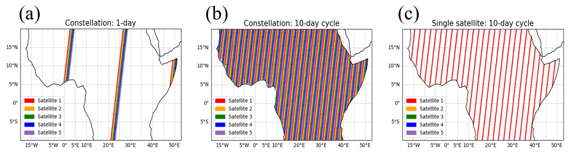
Figure 1 The ground track satellite coverage within our tropical African region: (a) the five-satellite NIMCAM constellation for the first day of the cycle, (b) the five-satellite NIMCAM constellation for the 10 d cycle, and (c) the in-orbit demonstrator NIMCAM concept for the 10 d cycle.

2.3 Sentinel 2 cloud probability data

We evaluated cloud interference using the Sentinel-2 cloud probability feature. Data retrieval was performed via the Google Earth Engine Python API (Gorelick et al., 2017). To maintain spatial consistency with our NIMCAM model, the 10 m data was resampled to 60 m, reprojected to the local UTM coordinate system, and exported in GeoTIFF format. We synchronised the temporal resolution with NIMCAM's 10 d repeat cycle, capturing three distinct data periods per month.

Cloud Probability (CP) is a common metric for quality masking in greenhouse gas retrievals. However, the literature reveals significant variation in established cutoff thresholds. For instance, Zhang et al. (2022) used a relaxed threshold for Sentinel-2 methane retrievals, considering an area cloud-free if the CP was below 65 % and filtering out scenes where more than 10 % of the region exceeded this limit. In contrast, studies of GOSAT-2 CO₂ and CH₄ observations adopted a more stringent filter, excluding all data with a CP>10 % (Suto et al., 2021). While reported limits in other studies span a broad range from 5 % to 70 % (Faruolo et al., 2023; Manninen et al., 2022; Declaro and Kanae, 2024), we have opted for a conservative 10 % limit. This strict threshold reflects the high-quality control likely required for NIMCAM observations and allows us to evaluate the specific advantages of NIMCAM's high horizontal resolution when operating under challenging cloud conditions, as found over tropical ecosystems.

We sample cloud information at the Sentinel-2 local solar time of equatorial crossing (10:30 LST), which may introduce a diurnal bias. To estimate the impact of this bias, we performed an analysis on the GEOS-FP cloud fraction dataset, which provides cloud information at a coarser horizontal resolution of 0.25°×0.3125°, but at a higher temporal resolution of every 3 h (Appendix, Fig. D1). Looking at cloud variability across the whole African region, cloud levels tend to be higher during the night, while during daylight hours they remain relatively stable. This suggests that cloud measurements taken at 10:30 LST do not exhibit a significant bias compared to other times of day. However, in the cloudiest region of tropical Africa, centred around the Congo Basin, there is a more distinct diurnal cycle during daylight hours. Cloud cover appears higher in the morning and evening, with a minimum occurring between 12:00 and 15:00 LST. In this region, cloud data extracted at 10:30 LST may slightly overestimate cloud levels at other times of day.

2.4 MODIS aerosol data

To characterise aerosol loading, we extract MODIS aerosol optical depth (AOD) in the green band (0.55 µm) at 1 km spatial resolution. Data were downloaded using the Earth Engine Python API in an analogous method to the cloud probability data extraction. MODIS has a 16 d repeat cycle, with additional data gaps due to quality screening. To maximise coverage, we aggregate the data over monthly periods. AOD is commonly used for quality masking in greenhouse gas retrieval studies, with thresholds typically ranging from 0.75 to 0.20 (Liu et al., 2024; Buchwitz et al., 2013; Li et al., 2022; Virtanen et al., 2024; Garrigues et al., 2022), and in some cases even more stringently with a threshold of 0.10 (Yu et al., 2024). For this study, we explore the more conservative thresholds, comparing the data availability for AOD cutoffs of 0.20 and 0.10. We downscale the 1 km MODIS AOD to the NIMCAM 60 m grid using a Gaussian probabilistic approach, described in Appendix C.

2.5 Translating raw EO data onto GEOS-Chem grid for atmospheric inversion studies

This approach follows the concept of “super observations”, in which multiple high-resolution retrievals are aggregated to the model grid scale (Eskes et al., 2003; Chen et al., 2023). The nested GEOS-Chem atmospheric chemistry and transport model (ACTM), described below, has a horizontal resolution of 0.25° (latitude)×0.3125° (longitude), which is coarser than the NIMCAM 60 m resolution. To assess the theoretical ability of NIMCAM to infer methane fluxes over tropical Africa, we count all available NIMCAM 60 m clear-sky scenes into the GEOS-Chem model grid boxes along the NIMCAM ground track swath within 10 d windows. They form the NIMCAM super observations.

To determine clear-sky NIMCAM scenes, we use the 60 m Sentinel-2 cloud probability dataset, and the downscaled 60 m MODIS AOD dataset, described above. The available NIMCAM pixel count is determined for the condition: CP<10 %, $\text{AOD}<\mathrm{0.1}.$ This translates to a NIMCAM dataset described on the GEOS-Chem modelling coordinate system, with the data availability at a temporal resolution of 1 h. We use this approach for the NIMCAM IOD and NIMCAM constellations, as described above. Within each GEOS-Chem model grid, there are up to 270 000 NIMCAM 60 m pixels available. Individual retrievals are assigned to GEOS-Chem grid cells based on their centre location, such that each observation contributes to a single grid box. Data were prepared for GEOS-Chem model runs to perform methane flux inversions.

2.6 The GEOS-Chem Atmospheric Chemistry Transport Model (ACTM) and the Ensemble Kalman Filter (EnKF)

Methane inversion experiments are conducted for April and October 2019, corresponding to the long and short rain seasons over East Africa, respectively (Palmer et al., 2023). Synthetic methane observations are generated for the NIMCAM IOD and the three- and five-satellite constellations, and consistently for the TROPOMI instrument.

We use the GEOS-Chem ACTM to describe the relationship between surface emissions of methane and observed changes in atmospheric methane. We use the nested version of the GEOS-Chem ACTM (version 13.4) to describe atmospheric methane within our tropical Africa domain (38° S–38° N, 20° W–55° E). The nested model uses a horizontal resolution of 0.25° (latitude) × 0.3125° (longitude) and is driven by the GEOS-FP meteorological analysis from the Global Modeling and Assimilation Office, based at NASA Goddard Space Flight Center (GSFC).

The prior simulations are forced by pre-defined anthropogenic and natural methane emission inventories, The natural methane fluxes include monthly wetland emissions covering rice paddies (Bloom et al., 2017); monthly fire emissions (van der Werf et al., 2017); and termite emissions (Fung et al., 1991). We also account for emissions from geological macroseeps (Kvenvolden and Rogers, 2005; Etiope, 2015). For anthropogenic emissions, we use the EDGAR v4.32 global emission inventory (Janssens-Maenhout et al., 2019), which includes a range of human-related sources such as the oil and gas sector, coal mining, livestock, and waste management. To represent the main oxidation sink of methane, we use monthly 3-D OH fields from the GEOS-Chem full-chemistry simulation (Mao et al., 2013; Turner et al., 2015), which are consistent with observed constraints on the lifetime of methyl chloroform.

The lateral boundary conditions are taken from a self-consistent global version of the ACTM but run on a coarser horizontal resolution of 2.0° (latitude) × 2.5° (longitude) using GEOS-FP meteorological reanalyses. This global model has been fitted to GOSAT proxy XCO₂ : XCH₄ retrievals (Feng et al., 2023). We use the posterior fluxes over Africa, inferred from these GOSAT data, as the truth in our OSSE to describe NIMCAM dry-air column methane mole fraction retrievals (XCH₄) in the GEOS-Chem ACTM. We assume that the prior flux estimates for the study region (10° S–20° N, 20° W–50° E) are the same as the prior inventories used by Feng et al. (2023). Our nested model region is larger than our study region to minimise the influence of lateral boundary conditions.

In the absence of real NIMCAM data, we use an OSSE configuration in which we define a “true” methane emission distribution that is used to determine the “true” 4-D distribution of atmospheric methane. We then sample that 4-D field as it would be observed by NIMCAM, considering its orbit, across-track measurement strategy, and the instrument averaging kernel that describe the instrument vertical sensitivity to changes in atmospheric methane (Appendix D2), and remove observed scenes according to CP<10 % and $\text{AOD}<\mathrm{0.1}.$ We add realistic sources of instrument noise to these NIMCAM “observations”, with a simple error model of 40 ppb for solar zenith angles (SZA) below 40° and 80 ppb for SZA above 40°. These values were derived from a detailed NIMCAM instrument performance and uncertainty analysis, including Monte Carlo propagation of instrumental, calibration, and systematic uncertainty sources through the retrieval measurement equation (Appendix B). To account for the reduced sensitivity of SWIR methane retrievals over water surfaces, the observation error is increased by a factor of two for grid cells where the GEOS-Chem FRLAND value is less than 50 %, which are treated as water bodies.

We then use these “observations” to infer posterior methane emission estimates using the GEOS-Chem ACTM, driven by a different methane emission distribution and an EnKF. For comparison, we use a similar approach to generate synthetic TROPOMI observations. The locations for the quality-filtered (qa>0.75) TROPOMI data are taken from an operational L2 XCH₄ product (Schneising et al., 2019, 2023). This OSSE follows an “identical twin” configuration, in which the same atmospheric transport model (GEOS-Chem) is used to generate synthetic observations and to perform the inversion. As a result, structural transport errors are not represented in this framework. This configuration is intentionally designed to isolate the role of observational sampling and measurement uncertainty; however, it represents an idealised scenario compared to real-world inversions.

We anticipate it is likely there will be many 60 m NIMCAM observations that fall within each GEOS-Chem nested model grid. In our OSSEs, we assimilate only one “super observation” for each model grid. To achieve this, we sample the GEOS-Chem model fields for each grid containing clear-sky NIMCAM observations (Sect. 3.1) and calculate individual values of XCH₄. This is done by convolving the resulting model methane profiles with an averaging kernel. The averaging kernels for NIMCAM are not fully characterised, so we assume values from GOSAT that vary with solar zenith angle and surface type. We assume the observation uncertainty δ for the NIMCAM super observations is described by:

$$\begin{array}{}\text{(1)}& {\displaystyle }{\displaystyle }\mathit{\delta }={\mathit{\delta }}_l+{\displaystyle \frac{{\mathit{\delta }}_{\text{GOSAT}}}{\sqrt{N}}},\end{array}$$

where δ_l is the uncertainty lower limit of 5 ppb, which describes sub-grid variations and scene-dependent biases, and N is the number of clean observations over land. The value of N is calculated as the number of 60 m NIMCAM clear-sky observations that fall within a grid's land fraction. This formulation assumes that individual retrieval errors are independent, such that the random component of the uncertainty decreases as $\mathrm{1}/\sqrt{N}$. In practice, this represents an upper bound on the achievable precision, as spatially correlated and scene-dependent errors (e.g. arising from surface reflectance, aerosols, and viewing geometry) will reduce the effective number of independent observations (N_eff<N). As a result, the uncertainty reduction achieved through aggregation may be weaker than implied by idealised $\mathrm{1}/\sqrt{N}$ scaling.

To infer posterior methane emission estimates from these atmospheric data, we use a modified version of Local Ensemble Transform Kalman Filter (LETKF) (Scarpelli et al., 2024). We use an ensemble of 91 flux perturbations at the model grid to represent the methane flux uncertainty over our study region. The prior uncertainty of methane fluxes is still challenging to quantify, with natural emissions often misallocated or even missing at the model grid resolution. Here, for simplicity, we define the prior uncertainty of the methane emission at each grid box by:

$$\begin{array}{}\text{(2)}& {\displaystyle }{\displaystyle }\mathit{\sigma }=\mathrm{0.2}({\mathbf{S}}_{\text{prior}}+[{\mathbf{S}}_{\text{prior}}-{\mathbf{S}}_{\text{post}}\left]\right),\end{array}$$

where S_prior and S_post denote the prior posterior emission estimate, respectively, from the corresponding global inversion (Feng et al., 2022). We assume the error correlation between grid boxes is 100 km, following previous studies (Scarpelli et al., 2024; Kurganskiy et al., 2025). The posterior error covariance is given by:

$$\begin{array}{}\text{(3)}& {\displaystyle }{\displaystyle }{\mathbf{S}}_{\text{post}}={\left({\mathbf{S}}_{\text{prior}}^{-\mathrm{1}}+{\mathbf{KS}}_{\text{obs}}^{-\mathrm{1}}{\mathbf{K}}^T\right)}^{-\mathrm{1}},\end{array}$$

where S_obs denotes the observational error covariance matrix, K denotes the Jacobian that describes the sensitivity of the observation (in this case, NIMCAM methane columns) to changes in surface emissions of methane.

We calculate the uncertainty reduction, to assess the theoretical potential of NIMCAM data:

$$\begin{array}{}\text{(4)}& {\displaystyle }{\displaystyle }\mathit{\eta }=\sqrt{\left(\mathrm{1}-{\displaystyle \frac{{\mathbf{S}}_{\text{post}}^{ii}}{{\mathbf{S}}_{\text{prior}}^{ii}}}\right)},\end{array}$$

where ${\mathbf{S}}_x^{ii}$ denotes the ith diagonal elements of the error covariance matrix.

3 Results

Here, we report all-sky and clear-sky data coverage statistics for the NIMCAM IOD and its constellation concepts and compare them against the performance of TROPOMI for the same synthetic atmosphere. We compare the co-added uncertainties associated with these NIMCAM and TROPOMI datasets after they are gridded onto the nested GEOS-Chem model grid. Finally, using a series of OSSEs, we examine the ability of these instruments to estimate “true” methane emissions.

3.1 All-sky data coverage statistics

We evaluate the data availability of NIMCAM methane observations (60 m resolution, 10 d repeat cycle) under three scenarios: as an IOD and as part of three- and five-satellite constellations. To provide context, these results were compared against the all-sky distribution of 7 km resolution data (equivalent to TROPOMI) and a 1 km resolution retrieval with a 5 d repeat cycle (representing a notional mid-resolution observing system.).

First, we consider all-sky methane retrievals aggregated onto 7 km grid cells with a temporal resolution of 10 d, corresponding to the approximate repeat time of the NIMCAM IOD. The number of potential NIMCAM retrievals is affected by the image resolution and the temporal resolution. For NIMCAM, the IOD only provides coverage of 19 % of the region over the 10 d period, while the three and five satellite constellations achieve 54 % and 89 % coverage, respectively (Fig. 2). In comparison, TROPOMI provides 100 % coverage daily due to its significantly larger across-track swath of 2600 km. In other words, daily TROPOMI all-sky coverage is comparable to 10 d of NIMCAM data collected by the five-constellation mission concept. At the 1 km resolution, we implement a 5 d repeat cycle, which translates to all-sky coverage every 5 d, and therefore 2 observations within each 10 d cycle.

Figure 2 Number of all-sky NIMCAM passes within each 7 km grid cell across the region during a 10 d cycle for the IOD and the three- and five-satellite constellation mission concepts. Coverage is defined as the proportion of 7 km grid cells with at least one satellite pass over the 10 d period. The IOD covers 18 % of grid cells, while the three- and five-satellite constellations increase coverage to 54 % and 89 %, respectively.

Within each 7 km grid cell, there are 13 611 NIMCAM pixels at 60 m resolution, 49 pixels at 1 km resolution, and a single pixel at 7 km resolution (nominally TROPOMI). However, the more frequent revisit times of the lower resolution data means that the number of retrievals per 10 d cycle increases to 98 and 10 for the 1 and 7 km resolution scenarios, respectively.

3.2 Clear-sky data coverage statistics

We now consider how cloud and aerosols affect the data availability at the different instrument retrieval spatial resolutions. Figure 3 shows the proportion of 7 km grid cells within our tropical African study region that are affected by cloud cover and elevated AOD (values of 0.1 and 0.2, as described above) for the four months of our study.

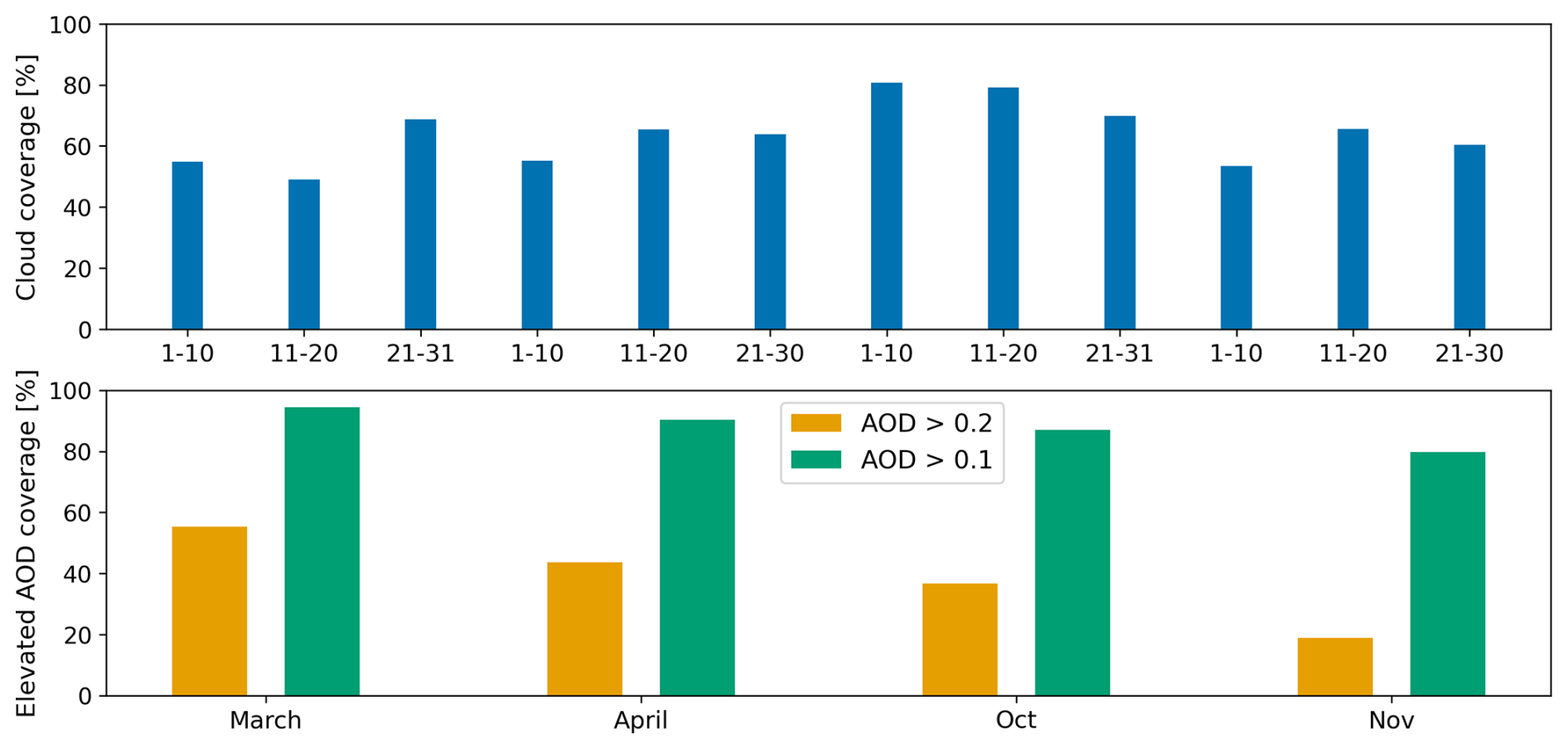
Figure 3 Monthly cloud coverage (top) and elevated AOD coverage (bottom) across our study region (10° S–20° N, mainland Africa) for March, April, October, and November 2019. Elevated AOD is shown for thresholds of 0.2 and 0.1.

October is the cloudiest month corresponding to the short rains season, with an average cloud coverage of 77 %. Most of the cloud cover is over the southern and mid-latitude areas including the tropical rainforest regions (Congo Basin, Guinean forests of West Africa, and eastern Afromontane). The cloud coverage is slightly lower for March, April, and November with an average coverage of 57 %, 62 %, and 60 %, respectively. Distributions of AOD loading over the regions are primarily influenced by seasonal biomass burning. Using an AOD threshold of 0.2, March exhibits the highest fraction of affected pixels (55 %), followed by April (44 %), October (37 %), and November (19 %). Using a stricter AOD threshold of 0.1, the corresponding values increase substantially, with March at 94 %, April at 90 %, October at 87 %, and November at 80 %. These results reflect the known seasonal cycle of biomass burning over Central and West Africa, which peaks during the late dry season in March–April and is lowest in November.

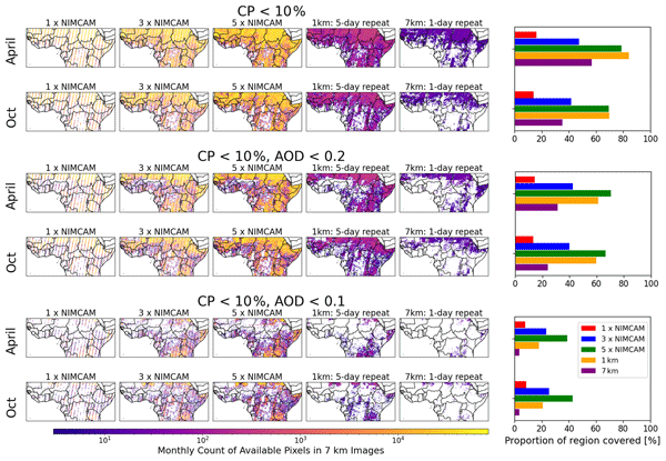
Figure 4 shows the spatial distribution of data availability following cloud masking (CP>10 %) alone, and combined cloud and aerosol masking using AOD thresholds of 0.2 and 0.1. All scenarios are evaluated on a common 7 km analysis grid, and data availability is quantified as the total number of clear-sky retrieval pixels accumulated within each 7 km cell over a 10 d observation window. We present results for April and October 2019 (with March and November shown in Appendix D3) for the NIMCAM IOD, and the 3- and 5-satellite NIMCAM constellations. NIMCAM observations are simulated at their native 60 m resolution and aggregated to the 7 km grid. For comparison, we also include a 1 km resolution, 5 d repeat scenario and a 7 km resolution, daily repeat scenario (nominally TROPOMI).

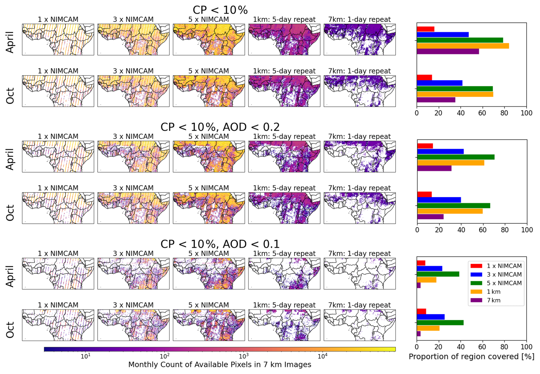
Figure 4 Total number of clear-sky retrieval pixels accumulated within each 7 km grid cell over a 10 d observation window for April and October. Results are shown for the NIMCAM IOD and the three- and five-satellite constellation mission concepts, a 1 km retrieval (5 d repeat), and a 7 km retrieval (daily repeat, nominally TROPOMI). Compared for cloud masking (CP<10 %) and AOD masking (thresholds 0.2 and 0.1). Bar charts indicate the proportion of 7 km grid cells with available data.

Looking at cloud masking alone, the NIMCAM IOD (single satellite) achieves the lowest fractional coverage, ranging from 10 %–15 % of the domain, as expected, reflecting its limited swath – in a clear-sky scenario the IOD only cover 18 % of the region. Three NIMCAM satellites improve coverage, while five NIMCAM satellites consistently surpass the TROPOMI scenario, and generally match or slightly underperform the 1 km scenario. Across all months, NIMCAM's high native spatial resolution of 60 m leads to 2–3 orders of magnitude more clear-sky pixels per 7 km cell compared to the TROPOMI case and 1 km mid-resolution scenario, as shown by the colour bar of monthly counts.

The benefits of NIMCAM's finer resolution are most evident in October, the cloudier of the two months studied. Here, three NIMCAMs outperform the TROPOMI scenario, and five NIMCAMs achieve comparable coverage to the 1 km scenario, despite the overall lower fractional coverage of the domain. Elevated cloud cover at TROPOMI resolution obscures almost the entirety of the African tropical rainforest regions, while NIMCAM's finer sampling spreads observations across a wider area of cells, reducing contiguous gaps and providing more spatially distributed information.

When additionally removing scenes with elevated AOD, data availability declines further, with the largest impacts observed in March and April and primarily affecting the northwest of the domain. At the moderate AOD threshold of 0.2, the NIMCAM IOD still shows the lowest coverage across all months, while three NIMCAM satellites surpass the TROPOMI scenario in every month except November. Additionally, the five-satellite NIMCAM constellation consistently outperforms the 1 km 5 d repeat scenario in all months except November.

Applying the stricter AOD threshold of 0.1 leads to a dramatic reduction in data availability for the TROPOMI scenario, with clear-sky coverage dropping to 4 % of the domain in March, April, and October, and 14 % in November. Under these conditions, NIMCAM's high-resolution observations become increasingly valuable. The single NIMCAM satellite now outperforms the TROPOMI scenario in all months except November, although its valid 7 km cells are more widely distributed across the domain, whereas the TROPOMI retains coverage primarily in the most northern areas. Three NIMCAM satellites exceed both the 1 km mid-resolution and TROPOMI scenarios in all months, including November, while the full five-satellite constellation achieves the highest coverage overall: April, 39 %; October, 42 %; March, 27 %; and November, 58 %.

These results demonstrate that the finer 60 m resolution of NIMCAM leads to a substantially more spatially extensive and distributed dataset, especially when clouds and aerosols remove large fractions of coarser-grid pixels. As data masking becomes stricter, the advantages of NIMCAM's high resolution and multi-satellite configurations become increasingly pronounced.

To evaluate the use of these satellite data for methane flux inversions (e.g. using GEOS-Chem and the ensemble Kalman filter, Sect. 3.4), we calculate the number of GEOS-Chem nested model grid boxes (0.25°×0.3125°) containing clear-sky observations for each 10 d study period. We compared the data density of TROPOMI against the NIMCAM IOD and the three-satellite and five-satellite constellations (Fig. 5). We find there are more observations for TROPOMI than the single NIMCAM IOD when we mask for clouds and use a AOD threshold of 0.2. However, when we adopt a stricter AOD threshold of 0.1 with the cloud masking, the NIMCAM IOD coverage exceeds TROPOMI across every 10 d period. The three-satellite and five-satellite NIMCAM constellations consistently outperform TROPOMI in grid-box availability. This relative advantage becomes more pronounced as the AOD masking criteria become more stringent. Using the 5-satellite constellation and our strict 0.1 AOD/cloud mask, NIMCAM provides up to 6 times more valid grid boxes than TROPOMI. These results demonstrate that NIMCAM's higher spatial resolution significantly enhances data availability, particularly in regions where strict quality filtering would otherwise limit observational coverage.

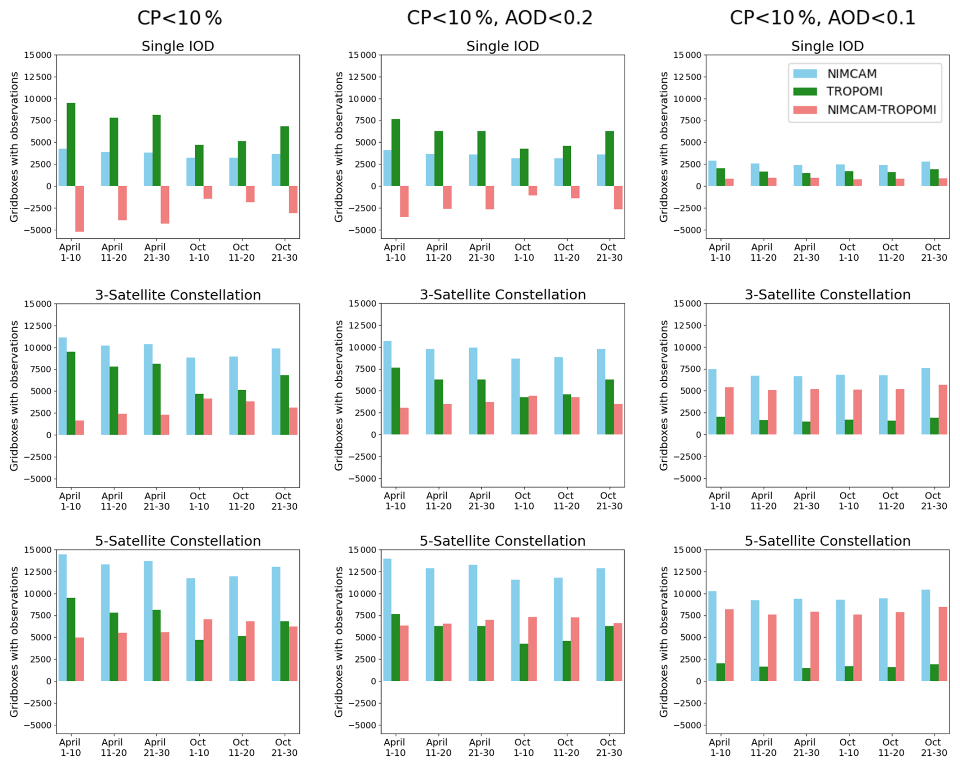
Figure 5 The number of GEOS-Chem nested model 0.25°×0.3125° grid boxes with available observations compared between NIMCAM (blue) and TROPOMI (green) and the difference (NIMCAM minus TROPOMI, red). Plotted for the 6, 10 d cycles through April, and October. Shown for a single NIMCAM IOD (top panel), a three-satellite constellation (middle panel), and the full five-satellite constellation (bottom panel). Compared when masking just for cloud (left panel), as well as cloud and AOD at 0.2 (middle panel) and AOD at 0.1 (right panel).

3.3 Improving the signal to noise of super observations of co-adding NIMCAM data

Here, we investigate how higher spatial resolution data influences random errors in accumulated methane super-observations on the GEOS-Chem nested model resolution of 0.25°×0.3125°. By comparing TROPOMI precision with estimated NIMCAM retrieval errors, mapped to the nested GEOS-Chem model grid over 10 d intervals, we quantify the impact of data co-addition. Under the assumption of uncorrelated noise, the random error scales by $\mathrm{1}/\sqrt{N}$, where N is the number of pixels contributing to each super-observation.

Analysis of TROPOMI CH₄ column data across our study region reveals an average single-pixel precision of 1.1 ppb (1.0–1.4 depending on the month). The NIMCAM single-pixel random error is estimated to be 40 ppb, based on radiative transfer simulations and retrieval algorithm modelling (Appendix B). Although this is more than an order of magnitude worse than TROPOMI at the single-pixel level, commensurate with the different science requirements, it is achieved at a substantially finer spatial resolution. The native NIMCAM pixel size is approximately 117 times smaller in linear dimension than TROPOMI, resulting in approximately 13 689 NIMCAM pixels per TROPOMI footprint. Conversely, TROPOMI provides approximately ten times higher temporal sampling than NIMCAM.

When aggregated to our GEOS-Chem nested model resolution of 0.25°×0.3125° over a 10 d window, the maximum potential sample size for NIMCAM reaches 273 780 pixels (468×585), whereas TROPOMI yields at most ∼200 measurements ($\mathrm{10}\mathrm{d}\times \sim \mathrm{20}$ pixels per day). The effective number of contributing pixels is further reduced by orbital coverage, such that the IOD, three-satellite, and five-satellite constellations sample approximately 18 %, 54 %, and 89 % of the grid, respectively.

These results are summarized in Table 2. Under ideal clear-sky conditions, the ratio of random error in NIMCAM super-observations to that of TROPOMI super-observations (${\mathit{\sigma }}_{\text{NIM}}/{\mathit{\sigma }}_{\text{TROP}}$) is 2.31, 1.33, and 1.04 for the IOD, three-satellite, and five-satellite constellations, respectively. This ratio metric is used in the following sections to assess how relative performance evolves under cloud and aerosol masking.

Table 2 Clear-sky comparison between NIMCAM (IOD, three-satellite, five-satellite) and TROPOMI, showing the average per-pixel error of retrievals, the number of potential observations per GEOS-Chem grid box in 10 d (N), and the corresponding error of the co-added super-observations.

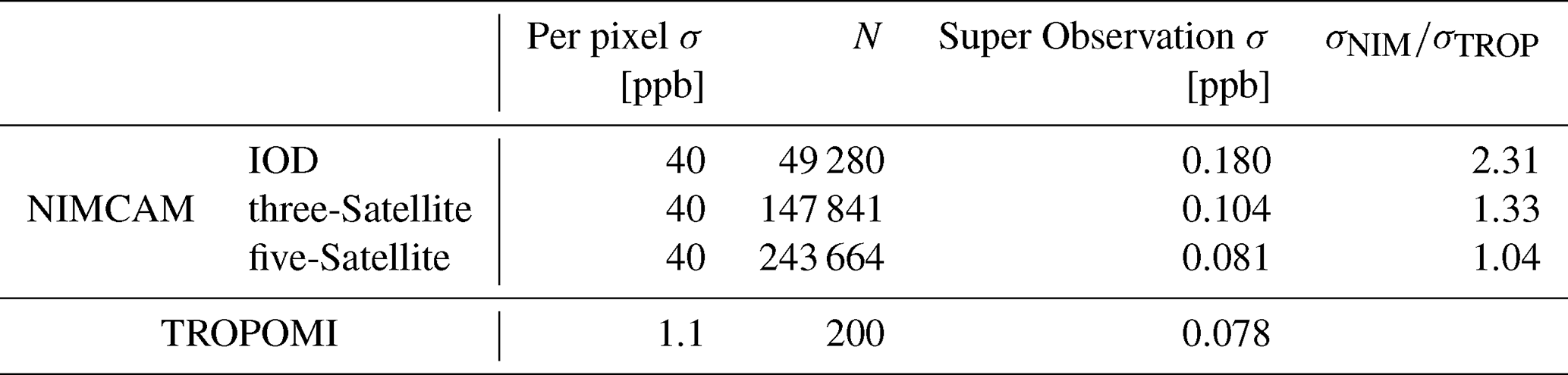
Figure 6 illustrates how the ratio between NIMCAM and TROPOMI super-observation random errors changes when progressively masking for clouds and aerosols. Across all scenarios, data masking leads to a proportionally larger increase in TROPOMI error relative to NIMCAM, such that the majority of grid cells exhibit error ratios lower than the corresponding clear-sky value (dashed line). This behaviour is particularly evident for the single-satellite IOD configuration, where the upper quartile of the distribution lies below the clear-sky reference across all time periods. This indicates that, despite its more limited spatial coverage, a single NIMCAM platform can still generate methane super-observations with random errors that remain competitive with those achieved by the three- and five-satellite constellations under realistic filtering conditions.

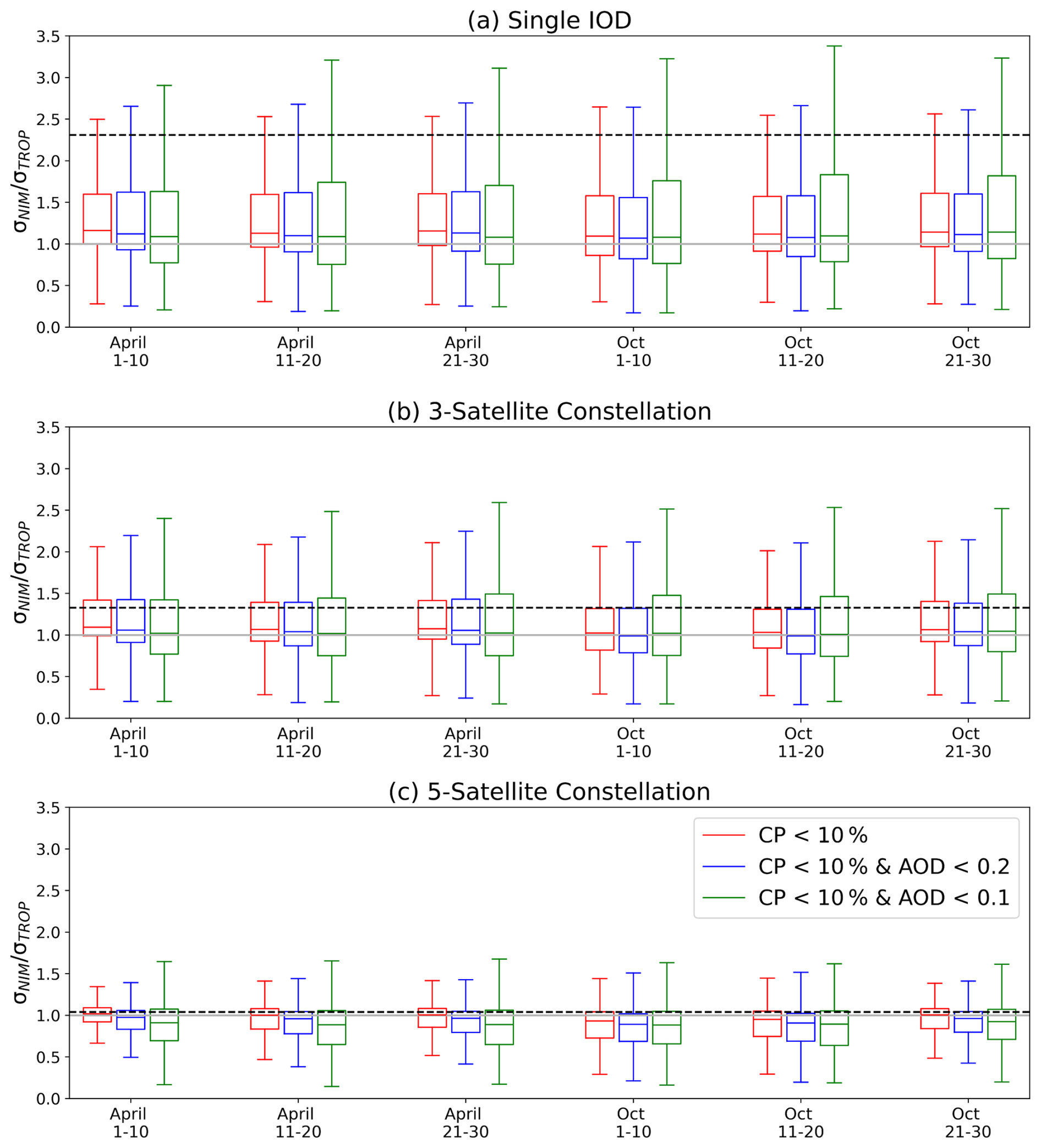
Figure 6 Statistical analysis of methane retrieval errors aggregated over a GEOS-Chem grid (0.25°×0.3125°) for 10 d intervals in April and October. Boxplots represent the NIMCAM/TROPOMI error ratio corresponding to cloud masking (red), and combined with AOD masking using thresholds of 0.2 (blue) and 0.1 (green). Presented for (a) Single satellite IOD, (b) the three-satellite constellation, and (c) the five-satellite constellation. Errors are modelled to scale by $\mathrm{1}/\sqrt{N}$, where N denotes the count of valid observations. The dashed horizontal lines in panels (a), (b), and (c) denote the baseline ratio of 2.31, 1.33, and 1.04, respectively, when all data are available.

Including AOD filtering in addition to cloud masking further enhances the relative advantage of NIMCAM, with the error ratio decreasing under AOD masking and showing additional reductions when applying the stricter AOD threshold of 0.1. Both the magnitude of the ratios and their overall trends are consistent between April and October, indicating that the behaviour is robust across seasons. Overall, these results demonstrate that high-resolution NIMCAM measurements are more resilient to data loss than TROPOMI. As cloud and aerosol filtering become increasingly stringent, NIMCAM exhibits a smaller relative degradation in effective sampling, leading to a slower growth in super-observation random error. The greatest overall benefit is seen for the 5-satellite constellation, where approximately 75 % of NIMCAM super-observations have smaller random errors than the corresponding TROPOMI super-observations (${\mathit{\sigma }}_{\text{NIM}}/{\mathit{\sigma }}_{\text{TROP}}<\mathrm{1}$) under the combined cloud and AOD filtering scenarios.

3.4 Estimating regional methane emissions using synthetic NIMCAM and TROPOMI data

Figure 7 show emission inversion estimates using simulated clear-sky observations of the NIMCAM IOD, the three and five NIMCAM constellation mission concepts, and TROPOMI for April 2019, respectively.

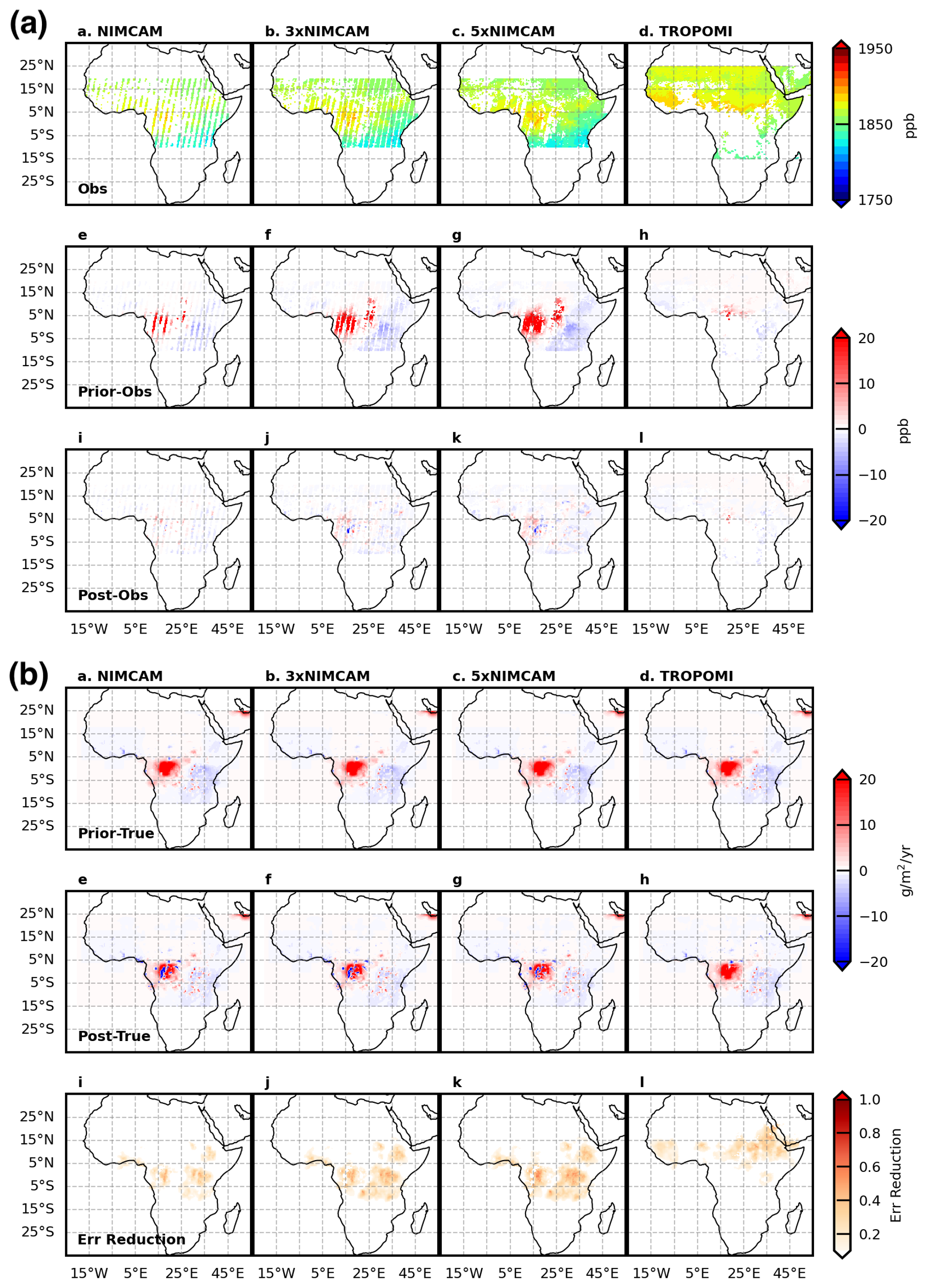
Figure 7 Synthetic methane emission inversion results for April 2019. (a) Simulated clear-sky XCH₄ observations for the NIMCAM IOD, three- and five-satellite NIMCAM constellations, and TROPOMI (top), with residuals relative to the prior (middle) and posterior (bottom). (b) Prior emission bias relative to the truth (top), posterior emission residuals (middle), and inversion fractional error reduction (bottom).

Compared to TROPOMI, the NIMCAM IOD shows data coverage across the study region instead of being focused over the broader Sahel region and Western Africa. The NIMCAM constellation fills in the observational gaps left by the IOD, with progressively more coverage over key methane-emitting regions, e.g. Congo Basin and the Sudd wetland regions in South Sudan. The biggest differences between the true values of XCH₄ and values corresponding to prior estimates are typically over the Congo Basin for the NIMCAM IOD and the constellations.

While XCH₄ differences for NIMCAM mission concepts are generally larger than those for TROPOMI, reflecting the larger retrieval random errors for NIMCAM, the density of NIMCAM super-observations provides a distinct advantage. In key regions where TROPOMI clear-sky data are sparse, the high volume of NIMCAM data significantly reduces the discrepancy between the posterior and the true emission estimates. Consequently, NIMCAM demonstrates significant theoretical potential to constrain methane emission estimates over tropical Africa during the rainy season, effectively filling critical observational gaps left by TROPOMI.

Figure 7b shows the corresponding improvements in the methane emission estimates in April. As expected, the posterior emission estimates are closer to the true values than the prior values. The NIMCAM IOD improves the emission estimates across many of the major methane-emitting regions, with performance improving progressively as the number of satellites in the constellation increases. The NIMCAM IOD outperforms TROPOMI for this month due to its ability to observe methane between clouds and between regions of elevated aerosol across the study domain. As a result, the uncertainty reduction, η, is generally larger for NIMCAM than for TROPOMI. We find that values of η begin to plateau after the three-satellite NIMCAM constellation, with only modest additional uncertainty reduction achieved by increasing the constellation size from three to five satellites. Although additional constellation members provide valuable data, the measurement uncertainty becomes small relative to errors associated with the atmospheric transport model. In other words, our ability to interpret these data is limited by the atmospheric transport model and not the data themselves.

Over the whole study region, the RMSE between the prior flux and the assumed true flux, calculated for all grid boxes with true emissions greater than 0.1 $\mathrm{g}{\mathrm{m}}^{-\mathrm{2}}{\mathrm{yr}}^{-\mathrm{1}}$, is 5.35 $\mathrm{g}{\mathrm{m}}^{-\mathrm{2}}{\mathrm{yr}}^{-\mathrm{1}}$. After assimilation, it decreases to 4.70, 3.78, 3.50, and 3.41 $\mathrm{g}{\mathrm{m}}^{-\mathrm{2}}{\mathrm{yr}}^{-\mathrm{1}}$ for the TROPOMI, one-, three-, and five-satellite NIMCAM observation systems, respectively. These correspond to overall reductions of 12.1 %, 29.3 %, 34.3 %, and 36.9 %, demonstrating substantial improvements from the NIMCAM observations but only modest additional benefit when increasing the constellation size from three to five satellites. The remaining errors are dominated by persistent overestimations in the Congo Basin, which are not fully constrained even by the five-satellite NIMCAM configuration. This highlights the challenges faced by space-based observations in regions where observational coverage is severely limited by persistently high cloud cover.

In addition, mismatches between the spatial patterns of the prior and assumed true fluxes limit the ability of neighbouring observations to correct emissions in these key regions. The assumed true fluxes are derived from a top-down inversion at coarse spatial resolution (hundreds of kilometres), resulting in spatially smoothed emission fields that can be displaced from their true locations and, in some cases, allocated over water bodies that cannot be observed by NIMCAM. Such discrepancies give rise to well-known challenges in LETKF inversions, including emission over- and underestimation and spatial misallocation. Consequently, part of the limited RMSE reduction reported here reflects the particularly demanding nature of the assumed truth scenario rather than limitations of the observing system alone. Nevertheless, mismatches between prior and true emission patterns are unavoidable in real-world LETKF applications, especially as inversion resolution increases and prior knowledge of local emissions becomes more uncertain. These limitations could be reduced through improved specification of prior uncertainties, particularly their spatial correlation structures, aided by the expanded observational constraints provided by future missions such as NIMCAM.

Figure 8 shows the same analysis but for October 2019 during the short rains across East Africa. Performance of NIMCAM is worse for this month due to more extensive cloud cover across the study region compared to April (Fig. 3). Similarly, the performance of TROPOMI is also worse for this month. After the NIMCAM data are ingested by the EnKF, we find that the posterior estimate is much closer to the truth, with substantial reductions over the Congo Basin. Unlike April, we find less evidence of the performance of the NIMCAM constellation plateauing after three satellites. This is because there are generally fewer clear-sky scenes, so the additional satellites are still providing valuable information to refine the methane emission estimates. This point is less obvious when we examine the posterior methane emission estimates. For this month the RMSE between the prior flux and the assumed truth, is 5.82 $\mathrm{g}{\mathrm{m}}^{-\mathrm{2}}{\mathrm{yr}}^{-\mathrm{1}}$. After assimilation, it decreases to 5.02, 3.66, 3.52, and 3.48 $\mathrm{g}{\mathrm{m}}^{-\mathrm{2}}{\mathrm{yr}}^{-\mathrm{1}}$ for the TROPOMI, one-, three-, and five-satellite NIMCAM observation systems, respectively. Again we see substantial improvements with high resolution NIMCAM observations but modest additional agreement from increased constellation size.

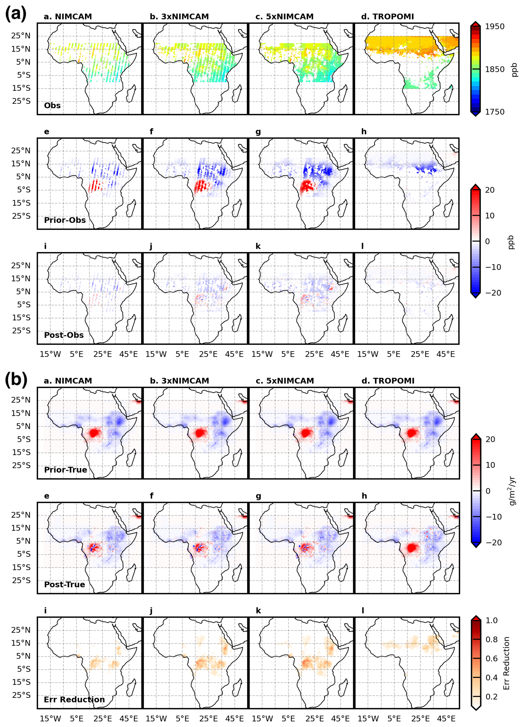
Figure 8 As Fig. 7 but for October 2019.

The results shown here assume idealised random errors in which individual retrievals are assumed to be independent and transport model error is not directly accounted for. These assumptions are used to isolate the role of observational sampling but represent a simplified inversion framework. A more realistic assessment could be achieved using a “fraternal twin” OSSE, in which different transport models are used to generate and invert the synthetic observations, thereby introducing structural model error. In practice, both transport errors and spatially correlated retrieval errors would reduce the effective information content of the observations and weaken the rate at which uncertainty decreases with increasing sampling density. The uncertainty reductions presented here should therefore be interpreted as a best-case (upper bound) estimate of achievable performance under realistic conditions. Nevertheless, the increased spatial coverage provided by high-resolution instruments such as NIMCAM remains a key advantage, particularly in regions where coarser-resolution observations provide limited valid data.

4 Concluding remarks

The results of this study underscore the unique capability of NIMCAM to bridge significant observational gaps in tropical methane monitoring. By using a high spatial resolution of approximately 60 m, NIMCAM can effectively view between fragmented cloud cover and regions of elevated aerosol optical depth that frequently obscure coarser area mappers like TROPOMI and GOSAT. In persistently cloudy regions such as the Congo Basin, where the kilometre-scale pixels of traditional sensors are often contaminated, NIMCAM's ability to retrieve clear-sky data between clouds ensures a more continuous and reliable record of wetland emissions.

While the signal-to-noise ratio of individual NIMCAM retrievals is significantly lower than that of larger flagship instruments, the high volume of clear-sky data points collected during peak emission seasons provides a robust statistical foundation for flux estimation. Our findings suggest that even conservative methane emission calculations derived from NIMCAM data offer substantial value, particularly in identifying diffuse sources within complex tropical ecosystems. The success of the NIMCAM in-orbit demonstrator further validates the mission concept and highlights the added value that a full constellation could provide in terms of temporal revisit frequency and global coverage.

We note that these results assume idealised error independence and should therefore be interpreted as an upper bound on achievable performance. Correlated retrieval errors would reduce, but not eliminate, the advantages associated with increased spatial sampling. Exploring sensitivity to different levels of correlated error would be a valuable avenue for future work.

More broadly, our study demonstrates the critical role that point source imagers play in the evolving global greenhouse gas observing system. As the field moves toward integrated multi-tiered architectures, the synergy between high-precision area mappers and high-resolution point source imagers will be essential for closing the methane budget. By providing the granular detail necessary to see between fragmented clouds and regions of elevated aerosol, instruments like NIMCAM, and the wider class of high-resolution satellite constellations, offer a scalable path to accurately quantify methane emissions from one of the world's most climate-critical regions.

Appendix A: NIMCAM spectral design and retrieval

NIMCAM uses three spectral channels. One channel is centred on a methane absorption feature at λ₁=1637.7 nm. The other two channels are located on either side of this at λ₂=1636.6 nm and λ₃=1638.7 nm and are designed to provide a measurement of surface reflectivity and absorption by other gases.

The observed intensity of reflected light through each channel C and in each pixel i is related to the surface reflectance, r_C, the incident solar radiation intensity integrated over the spectral channel, $I_{{\text{solar}}_C}$, the channel absorption cross section, σ_C, the methane slant column density, SCD, and the absorption due to background levels of gases, τ_bkg as follows:

$$\begin{array}{}\text{(A1)}& {\displaystyle }{\displaystyle }{I}_C^i=r_C{I}_{{\text{solar}}_C}{\mathrm{e}}^{-{\mathit{\sigma }}_C\text{SCD}-{\mathit{\tau }}_{\text{bkg}}}\end{array}$$

The per channel per pixel intensities $I_C^i$ are calculated from the per-pixel electron count measured during a single exposure. The intensity in Watts per pixel is calculated by division of the electron count, $N_C^i$ by the detector quantum efficiency at the channel wavelength, QE_C, and multiplication by the photon energy at the same wavelength, E_C. Images are captured using a Indium Gallium Arsenide Short-Wave Infrared detector, the noise characteristics of which lead to the addition of a random electron noise $\mathrm{\Delta }{N}_C^i$ as described in more detail below.

$$\begin{array}{}\text{(A2)}& {\displaystyle }{\displaystyle }{I}_C^i={\displaystyle \frac{(N_C^i+\mathrm{\Delta }{N}_C^i)E_C}{{\text{QE}}_C}}\end{array}$$

Detector noise (shot noise, readout noise, and dark current) is reduced via a co-addition observation scheme, where the detector frame rate is arranged such that n_along-track observations are collected for each spatial pixel, with $n_{\text{along-track}}/\mathrm{3}$ observations contributing to each of the channel averaged intensity values I_C which are calculated as follows:

$$\begin{array}{}\text{(A3)}& {\displaystyle }{\displaystyle }{I}_C={\displaystyle \frac{{\sum }_{i=\mathrm{1}}^{n_{\text{along-track}}/\mathrm{3}}{I}_C^i}{n_{\text{along-track}}/\mathrm{3}}}\end{array}$$

n_along-track is the number of pixels in the long side of the detector pixel array; this side is aligned with the instrument flight direction. For the selected camera n_along-track=640.

A linear fit to the spectrum of the surface reflectance is assumed, and differential absorption due to background gases is not considered separately but rather included in the linear fit of the surface reflectance signal. This allows the absorption due to τ_bkg to be removed. The surface reflectance is interpolated to give r₁:

$$\begin{array}{ll}{\displaystyle }& {\displaystyle }{r}_{\mathrm{1}}({\mathit{\lambda }}_{\mathrm{3}}-{\mathit{\lambda }}_{\mathrm{1}})-r_{\mathrm{2}}({\mathit{\lambda }}_{\mathrm{3}}-{\mathit{\lambda }}_{\mathrm{1}})=r_{\mathrm{3}}({\mathit{\lambda }}_{\mathrm{1}}-{\mathit{\lambda }}_{\mathrm{2}})-r_{\mathrm{1}}({\mathit{\lambda }}_{\mathrm{1}}-{\mathit{\lambda }}_{\mathrm{2}})\\ {\displaystyle }& {\displaystyle }{r}_{\mathrm{1}}({\mathit{\lambda }}_{\mathrm{3}}-{\mathit{\lambda }}_{\mathrm{2}})=r_{\mathrm{3}}({\mathit{\lambda }}_{\mathrm{1}}-{\mathit{\lambda }}_{\mathrm{2}})+r_{\mathrm{2}}({\mathit{\lambda }}_{\mathrm{3}}-{\mathit{\lambda }}_{\mathrm{1}})\\ {\displaystyle }& {\displaystyle }{r}_{\mathrm{1}}={\displaystyle \frac{\mathrm{1}}{{\mathit{\lambda }}_{\mathrm{3}}-{\mathit{\lambda }}_{\mathrm{2}}}}\left(\right({\mathit{\lambda }}_{\mathrm{1}}-{\mathit{\lambda }}_{\mathrm{2}})r_{\mathrm{3}}+({\mathit{\lambda }}_{\mathrm{3}}-{\mathit{\lambda }}_{\mathrm{1}}\left)r_{\mathrm{2}}\right)\end{array}$$

Substituting for r using the Beer–Lambert law:

$$\begin{array}{ll}{\displaystyle }& {\displaystyle \frac{I_{\mathrm{1}}}{I_{{\text{solar}}_{\mathrm{1}}}}}{\mathrm{e}}^{{\mathit{\sigma }}_{\mathrm{1}}\text{SCD}}{\mathrm{e}}^{{\mathit{\tau }}_{\text{bkg}}}={\displaystyle \frac{\mathrm{1}}{{\mathit{\lambda }}_{\mathrm{3}}-{\mathit{\lambda }}_{\mathrm{2}}}}[{\displaystyle \frac{I_{\mathrm{3}}({\mathit{\lambda }}_{\mathrm{1}}-{\mathit{\lambda }}_{\mathrm{2}})}{I_{{\text{solar}}_{\mathrm{3}}}}}{\mathrm{e}}^{{\mathit{\sigma }}_{\mathrm{3}}\text{SCD}}{\mathrm{e}}^{{\mathit{\tau }}_{\text{bkg}}}\\ {\displaystyle }& {\displaystyle }+{\displaystyle \frac{I_{\mathrm{2}}({\mathit{\lambda }}_{\mathrm{3}}-{\mathit{\lambda }}_{\mathrm{1}})}{I_{{\text{solar}}_{\mathrm{2}}}}}{\mathrm{e}}^{{\mathit{\sigma }}_{\mathrm{2}}\text{SCD}}{\mathrm{e}}^{{\mathit{\tau }}_{\text{bkg}}}]\\ {\displaystyle }& {\displaystyle \frac{I_{\mathrm{1}}}{I_{{\text{solar}}_{\mathrm{1}}}}}{\mathrm{e}}^{{\mathit{\sigma }}_{\mathrm{1}}\text{SCD}}={\displaystyle \frac{\mathrm{1}}{{\mathit{\lambda }}_{\mathrm{3}}-{\mathit{\lambda }}_{\mathrm{2}}}}[{\displaystyle \frac{I_{\mathrm{3}}({\mathit{\lambda }}_{\mathrm{1}}-{\mathit{\lambda }}_{\mathrm{2}})}{I_{{\text{solar}}_{\mathrm{3}}}}}{\mathrm{e}}^{{\mathit{\sigma }}_{\mathrm{3}}\text{SCD}}\\ \text{(A4)}& {\displaystyle }& {\displaystyle }+{\displaystyle \frac{I_{\mathrm{2}}({\mathit{\lambda }}_{\mathrm{3}}-{\mathit{\lambda }}_{\mathrm{1}})}{I_{{\text{solar}}_{\mathrm{2}}}}}{\mathrm{e}}^{{\mathit{\sigma }}_{\mathrm{2}}\text{SCD}}]\end{array}$$

The values of $I_{{\text{solar}}_{\mathrm{1}}}$, $I_{{\text{solar}}_{\mathrm{2}}}$, and $I_{{\text{solar}}_{\mathrm{3}}}$ are calculated from a known solar spectrum convolved with the measured channel transmission curves of the as-manufactured filters. The values of σ₁, σ₂, and σ₃ are calculated by convolving the same channel transmission curves with the methane absorption cross section. The values of λ₁, λ₂, and λ₃ are specified for each filter and then measured after manufacture. Equation (A4) is then solved numerically for SCD.

Appendix B: NIMCAM uncertainty

The NIMCAM vertical column density (VCD) (single pass slant column density (SCD)) uncertainty performance calculations were initially performed “per pixel” approximately 60 m ground sampling distance, including along-track co-adding across the filter elements. Figure B1 shows the VCD uncertainty (expressed as ppb and %) as a function of methane enhancement (ppb) characterised as independent (random), structured and common (systematic) together with their totals, where the characterisation follows the Quality Assurance Framework for Earth Observation (QA4EO).

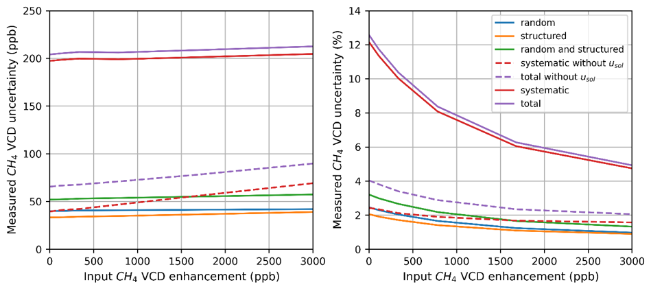
Figure B1 NIMCAM VCD “per pixel” uncertainty contributions (left, in ppb and right, as a percentage) separated into random (noise) [blue], structured (largely thermal effects on a per orbit timescale) [orange], globally systematic components [red] and total [purple] as a function of methane enhancement (ppb). Additional curves show the combined random and structured term [green], together with the systematic and total uncertainties without the literature solar irradiance (Usol) uncertainty included (red and purple dashed, respectively).

The primary source of random uncertainties is in the instrument noise, dominated by shot noise with small contributions from dark current and readout noise components (for the uncertainty calculation it is assumed the instrument transmission has been optimised for the maximum signal – no methane enhancement – to be ∼80 % of the detector Full Well Capacity (FWC) for the measured double pass SCD). The structured components are temperature-dependant terms acting on an orbital timescale dominated by filter spectral and transmission components. The common sources are dominated by pre-flight characterisation, species cross-section and solar irradiance reference knowledge alongside optical degradation assumption uncertainties. A full uncertainty budget estimation is not presented here but has been prepared for a sister, performance-led publication.

The SCD uncertainty is calculated via a Monte Carlo approach through inputting of the SCD measurement equation, variables and uncertainty in the punpy function of the NPL Community Metrology (CoMet) toolkit (De Vis and Hunt, 2026). The SCD measurement equation effectively divides the uncertainty terms into two groups, those linear with SCD (related to the species cross-sections so manifest relatively invariant in absolute terms to methane concentration) and the group outside the exp() term proportional to measured/transmitted signal and reference solar irradiance (that experience a significant up-tick in uncertainty for low methane enhancements).

The per pixel uncertainty is most relevant for an instantaneous imaging application, whereas for an inversion application the spatial and temporal averaging (alongside the cal/val strategy) need to be considered to estimate suitable uncertainties.

The structured uncertainty components are predominantly temperature-dependent and have been assessed to vary most strongly on an orbital scale. Aided by the sun synchronous orbit, on the averaging scale of daily, weekly and beyond these components will increasingly manifest randomly, so can be combined with the random component in Fig. B1 [green curve]. Over a typical 25 km footprint used in the inversion approximately 105 pixels will be averaged reducing the revised random per pixel uncertainty from ∼40 to <1 ppb (for near background level concentrations).

The higher ∼200 ppb per pixel systematic contribution for background methane levels is primarily attributed to pre-flight characterisation, in-flight differential channel degradation correction residual and reference value knowledge. These can be characterised and overwhelmingly corrected for in-flight through calibration and validation activities.

The details of in-flight calibration activities (sun-viewing operations) to quantify and monitor differential channel degradation correction and reference solar irradiance assumptions will not be expanded upon here, but do allow some separation of these terms in flight. The narrow spectral range in which the NIMCAM channels reside allow a common treatment of these systematic effects, significantly reducing their magnitude. The dominant nature of the reference solar irradiance uncertainty ($u_{I_{\text{sol}}}$) (∼160 ppb) is highlighted in Fig. 1, in that without it the per pixel systematic terms drop to ∼40 ppb (for near background methane concentrations). All the contributors are truly globally systematic, except for any differential channel transmission degradation that would evolve during the mission lifetime and required a routine solar calibration and validation activities to monitor and correct for.

The primary strategy to reduce systematic uncertainty will be addressed via validation against the TCCON network. The Total Carbon Column Observing Network (TCCON) measures column-average mole fractions of several greenhouse gases (GHGs), beginning in 2004, from over 30 current or past measurement sites around the world using solar absorption spectroscopy in the near-infrared (near-IR) region (Wunch et al., 2011). Validation against TCCON is a mature activity common to GHG satellite missions (e.g. Lorente et al., 2021). For the GGG2020 version, the XCH₄ uncertainties are quoted at approximately 0.2 % (4 ppb) for SZA<75°, rising to 0.4 % (7 ppb) at SZA ∼82° (Laughner et al., 2024).

To use TCCON to derive the overall bias, the random components need to be reduced to below the required correction level, but this has previously been shown to be met by a single 25 km footprint. The orbitx package (based on Orekit Journot et al., 2018) of the NPL Metrology for Earth Observation and Radiometry (MetEOR) toolkit (De Vis and Hunt, 2026) was used to determine the frequency of observations of the TCCON sites for a nominal NIMCAM sun-synchronous orbit (10:30 LTDN, 600 km altitude and 25 km instrument swath). For a coincidence distance of 250 and 400 km radius to the TCCON site, limited to SZA<75°, the total number of potential annual observations over all TCCON sites is approximately N₂₅₀=3692 and N₄₀₀=5748 respectively. The experience of other missions is that 10 %–20 % of potential observations pass cloud clearing and other quality checks (e.g. Parker et al., 2020) suggesting Ngood ∼ 500–800 opportunities per year. Whilst a recent example with OCO-2 validation against TCCON would suggest greater pessimism should be employed for the strictest coincident measurement quality criteria (Das et al., 2025), this level of observation statistics should be suitable for an initial bias correction one year into the mission. Typical validation convergence against TCCON achieves a mean bias estimation and sd. dev. of ≤5 ppb, although TCCON station to station variation has been seen to be nearer ±10 ppb with a st. dev. of 20 ppb (Lorente, 2021). For this study the residual (post-correction) systematic bias, for averaged over all TCCON sites has been taken as 5 ppb.

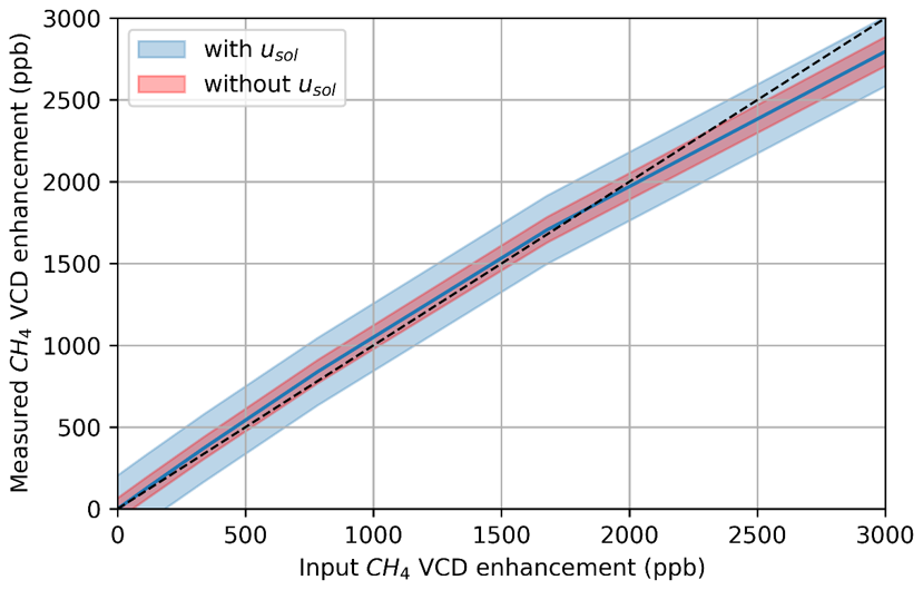
Figure B2 Simulated NIMCAM instrument VCD measurement linearity to input enhancement. The error bars show the total uncertainty [blue shading] (purple curve in B1) and total uncertainty.

Figure B2 shows the simulated measured VCD enhancement against input VCD enhancement for the NIMCAM instrument for methane enhancements up to 3000 ppb. The plot shows good linearity for low enhancements, with some underrepresentation at higher concentrations. The shape of the curve is a consequence of an assumed detector channel linear response to methane enhancement when in reality some nonlinearity in the absorption feature grown exists, that could be addressed with pre-flight characterisation activities.

Appendix C: Probabilistic sub-grid inference of MODIS AOD

To relate MODIS AOD at 1 km resolution to the NIMCAM horizontal resolution of 60 m, we adopt a probabilistic downscaling approach to estimate the number of 60 m pixels with AOD below a given threshold within each 1 km grid cell. For each 1 km cell, we compute a local standard deviation (σ) from the variability of AOD in neighbouring grid cells, which serves as an estimate of sub-grid variability. The reported AOD value is treated as the mean (μ) of a Gaussian distribution. The probability of a 60 m NIMCAM pixel within each 1 km grid cell having AOD below a certain threshold T (e.g. 0.2 or 0.1) is determined by applying the cumulative distribution function (CDF) of the Gaussian distribution:

$$\begin{array}{}\text{(C1)}& {\displaystyle }{\displaystyle }P(\text{AOD}<T)=\mathrm{\Phi }\left({\displaystyle \frac{T-\mathit{\mu }}{\mathit{\sigma }}}\right),\end{array}$$

where Φ is the CDF of the standard normal distribution. If σ=0, all sub-grid pixels are assumed to have identical AOD, and the probability is set to 0 or 1 depending on whether μ is below the threshold. Once the probability is calculated, the number of 60 m NIMCAM pixels expected to have AOD below the threshold is found by multiplying the probability by the total number of 60 m NIMCAM pixels in each 1 km cell.

We test our Gaussian assumption by using 15 samples of 60 m resolution AOD product based on Sentinel-2 imagery, processed over northern Ghana. Overall, we find our approach effectively predicts the fraction of AOD-free 60 m pixels from 1 km AOD. Figure C1 summarises the correlation coefficients and biases for all 15 samples. Correlations remain consistently high, with median values of 0.95 and 0.97 for the 0.1 and 0.2 thresholds, respectively. Biases are small, with a median of −0.02 for both thresholds. The bias is predominantly negative, indicating a slight overestimation of the number of AOD-free pixels.

Figure C2 shows the analysis on two representative cases of low and high AOD images. The fraction of AOD values below the two thresholds (0.2 and 0.1) within each 1 km grid was computed directly from the the high-resolution 60 m AOD data. Additionally, the 60 m images were downsampled to 1 km resolution, and the fraction of AOD below these thresholds was estimated using the Gaussian approach described above. The observed and predicted fractions exhibit very visually similar distributions, with high correlations and minimal bias.

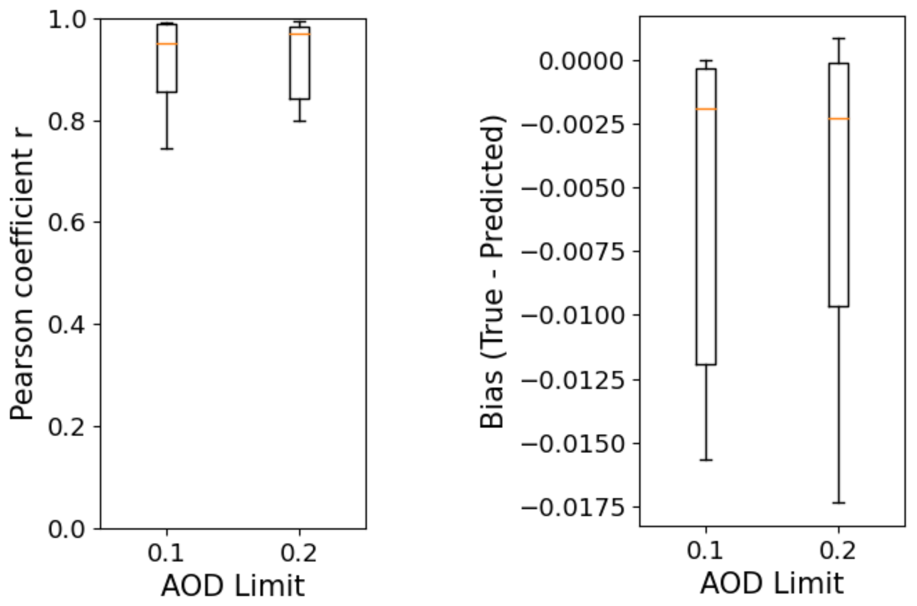
Figure C1 Boxplots showing the range in Pearson correlation, r and mean bias for the 15 processed images.

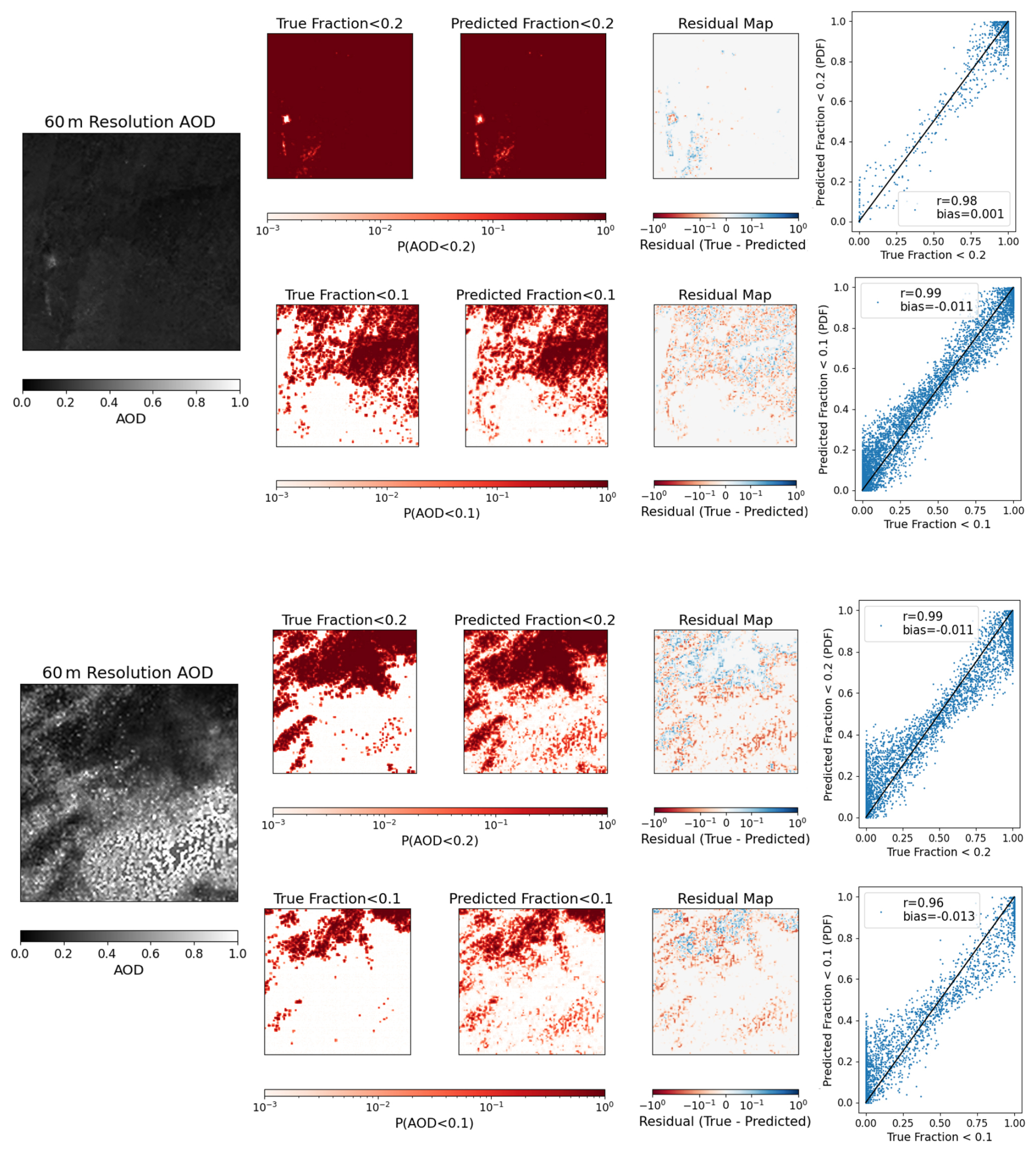
Figure C2 Two examples of high resolution AOD at 60 m. The images are gridded onto a 1 km grid and the actual fraction of data <0.2 and <0.1 are counted in each grid. The images are then downsampled to 1 km resolution and the fraction of data <0.2 and <0.1 are predicted using a CDF with Gaussian distribution. The residual map, and scatter plot shows the difference between the true and predicted fractions.

Appendix D

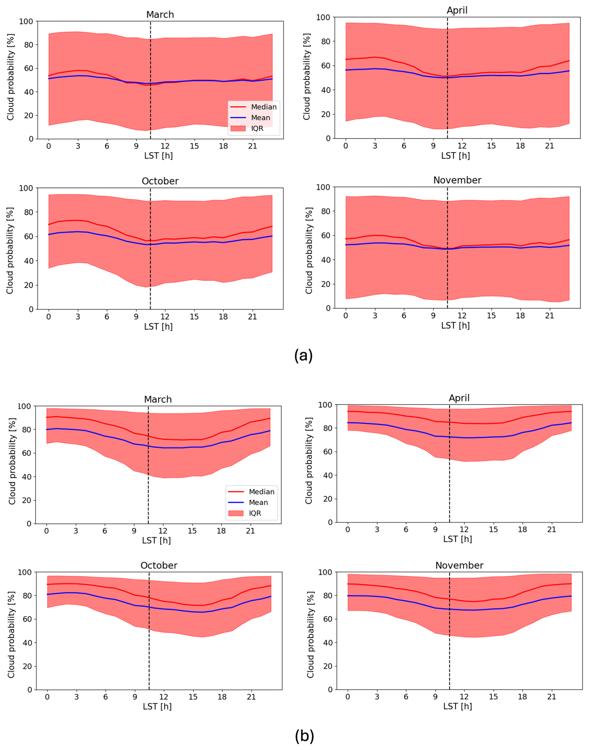
Figure D1 The diurnal variability in cloud coverage from the GEOS Forward Processing (GEOS-FP) dataset, which provides cloud information at 3 hourly temporal resolution on a 0.25°×0.3125° spatial resolution. Median (red line), mean (blue line) and IQR (red shaded) cloud fraction plotted against local solar time (LST). Black dashed line marks 10:30, the mean LST of Sentinel-2 overpass (a) Shows the cloud coverage averaged across the full African region, (b) shows the cloud coverage over the Congo Basin (Lat: $[-\mathrm{7},\mathrm{4.5}]$, Lon: [11.5,30]), which is one of the cloudiest regions in tropical Africa.

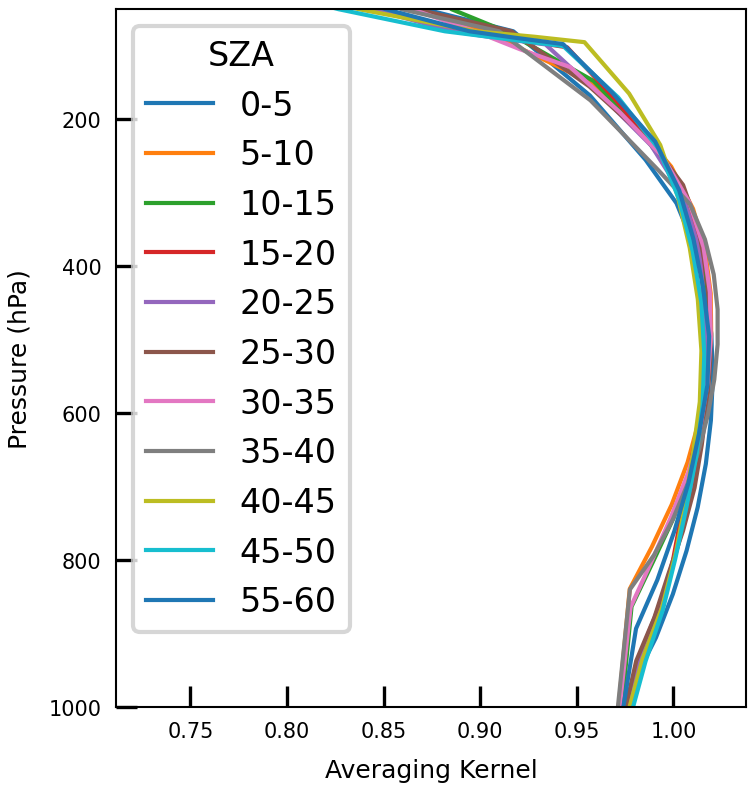
Figure D2 Averaging Kernel profiles used for both NIMCAM and TROPOMI synthetic methane observations. 11 profiles shown binned by solar zenith angle (SZA). Taken from proxy GOSAT XCH₄ retrievals over land.

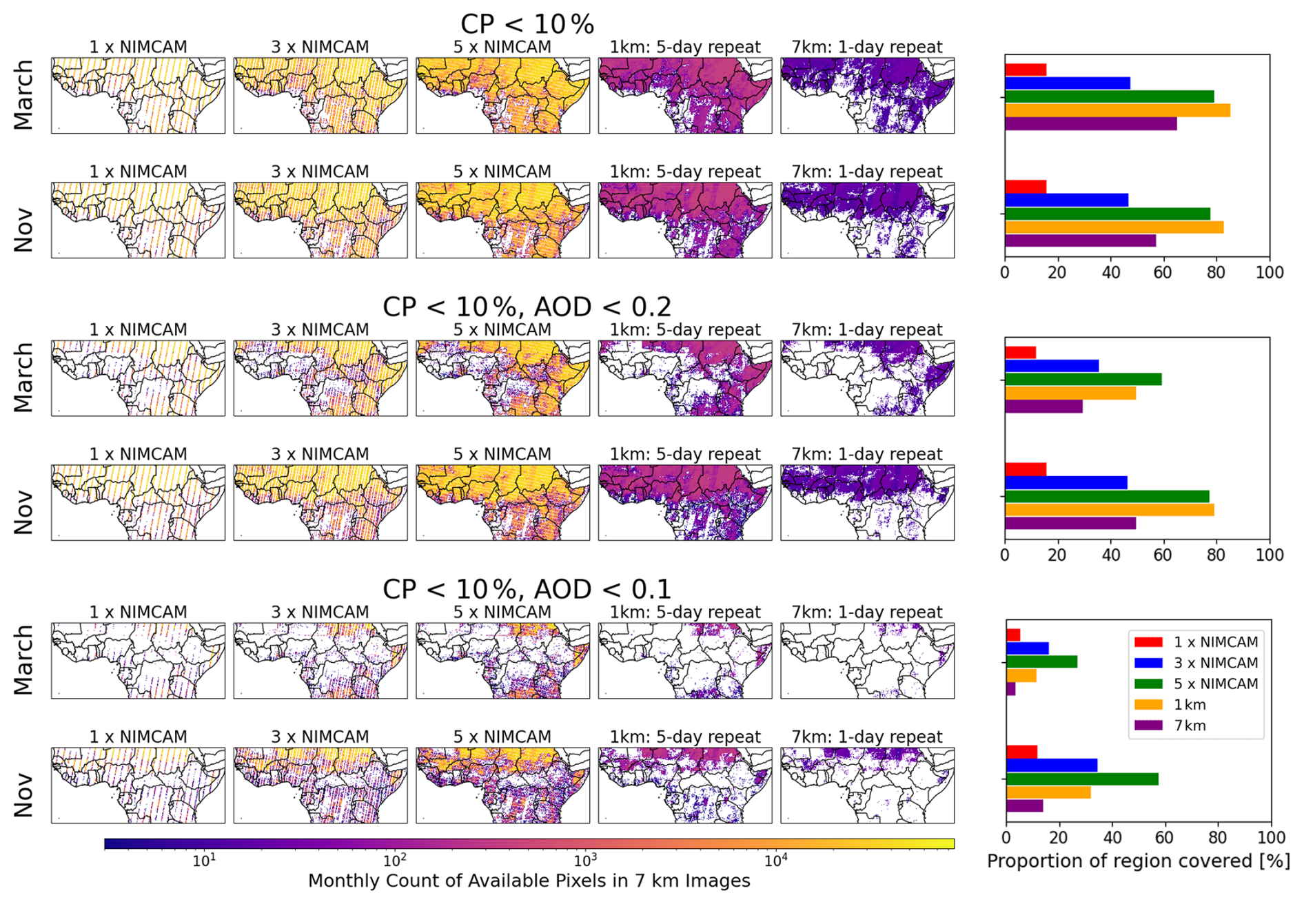
Figure D3 Total pixels recorded in March and November for the NIMCAM IOD and the three and five constellation mission concepts, 1 km retrieval (5 d repeat), and 7 km retrieval (daily repeat, TROPOMI). Compared for cloud masking (CP<10 %) and AOD masking (thresholds 0.2 and 0.1). Bar charts show the image availability proportion.