SPS30 and SEN55 PM_2.5 sensor intercomparison and validation through indoor and outdoor measurements in Arba Minch, Ethiopia

Ethiopian air pollution is understudied yet highly relevant considering population size and source abundance including solid fuel cooking, small scale waste burning and vehicle fleet. Low-cost PM_2.5 sensors can be used to mitigate this by mapping pollution exposure. We report on indoor and outdoor measurements with Sensirion sensors SPS30 and SEN55, the former extensively validated in literature, the latter not. We evaluate their use in Arba Minch, population ca. 200 000. In addition to sensor inter and intra comparison we benchmark the low-cost sensors against gravimetry. Furthermore, a separate Swedish outdoor dataset is included to extend the range of particle types and loadings and evaluate relative humidity (RH) effects using a reference-equivalent monitor (Palas FIDAS).

We found that the SEN55 consistently reports values 6 %–10 % higher than the SPS30; once this systematic offset is corrected, the sensor types are functionally identical with high precision (coefficient of variation ≤7.7 %, between-sampler uncertainty ≤1.7 µg m⁻³). Both sensors demonstrated high stability across repeated high-concentration events (>1000 µg m⁻³). While the SEN55 exhibits digital truncation at 6553.4 µg m⁻³, we find that measurements beyond the 1000 µg m⁻³ manufacturer specification remain meaningful and essential for accurate mass estimation in biomass-burning environments. The impact of relative humidity was small and consistent across both sensor types.

Our study shows that the SPS30 and SEN55 – when calibrated under circumstances of use – are stable and accurate instruments (indoor and outdoor accuracy error ≤22 %, outdoor expanded uncertainty ≤15 % in comparison to gravimetric measurements). Pragmatic, large-scale low-cost monitoring supported by mobile gravimetric validation offers the most viable path toward mitigating air pollution exposure in resource-constrained settings.

1 Introduction

The relationship between air quality and public health is well-documented, with PM_2.5 exposure directly linked to increased mortality and cardiorespiratory disease (Anderson et al., 2012; World Health Organization, 2021). The global burden of these health impacts is highest in low-income countries (World Health Organization, 2024, 2025). For a low-income country like Ethiopia, this problem is two-fold: outdoor air pollution related to open waste burning and relatively older vehicles, and indoor air pollution related to use of biomass fuels (which also contributes to outdoor air pollution).

Addressing PM_2.5 exposure is further hindered by resource limitations, leading to a lack of monitoring infrastructure. As air pollution varies across both space and time, high-resolution monitoring networks are needed for identifying pollution peaks and pinpointing human exposure (Karagulian, 2023; Li et al., 2020; Maji et al., 2017; Mushtaq et al., 2024). The reference method for PM_2.5 monitoring (gravimetry) and reference equivalent monitors are expensive regarding labour and material costs, hence generally not a feasible solution for low-income countries. In recent years, however, low-cost sensors (LCS) are gaining traction as a viable alternative to traditional regulatory sites (Karagulian et al., 2019; Kumar et al., 2015; Suriano and Prato, 2023). Their low investment and maintenance costs make it feasible to set up dense networks (Kumar et al., 2015; Morawska et al., 2018). LCS are commonly sold as pre-assembled systems, but additional cost reduction is achieved by sourcing sensors from original equipment manufacturers (OEMs) for local assembly.

Light-scattering LCS introduce inherent data quality uncertainties regarding precision (consistency between identical units) and accuracy (proximity to “the truth”). The relationship between light scattering and mass concentration to particle composition and shape varies across particle types. The accuracy of a sensor, without changing scatter to mass translation, might be good under one condition, while underperforming under another. This necessitates local validation under site-specific conditions rather than relying only on factory calibrations (Karagulian et al., 2019). Furthermore, sensor quality affects both the precision and accuracy, which varies from sensor type to sensor type. It is therefore important to validate specific sensor types, rather than to let one low-cost sensor type stand as representative of others. A specific metric of sensor quality is its performance under high particulate loads, often used as a proxy for long-term stability (Tryner et al., 2020). This is particularly relevant in the Ethiopian context, where indoor environments frequently reach high concentrations (Admasie et al., 2019; Dingemanse and Tademe, 2023; Tamire et al., 2021). Finally, humidity affects the accuracy of the scatter-to-mass translation. Increased relative humidity can lead to scattering enhancement (Zieger et al., 2013) due to hygroscopic particle growth and changed optical properties (Liu et al., 2019). The κ-Köhler theory can be used to make a physical correction for the effect of hygroscopic particle growth when particle composition is constrained (Malings et al., 2020; Tryner et al., 2020). Others make non-physical correction with RH as variable within regression analyses (Malings et al., 2020; Zusman et al., 2020).

Among OEM sensors, the Sensirion SPS30 has become popular (Wesseling et al., 2024) and is frequently selected for its precision, accuracy and durability (Gabriel and Auer, 2023; Mahajan, 2022; Mujan et al., 2021; Park et al., 2021a, b; Riediker, 2022). Comparative studies often rank the SPS30 above others in terms of accuracy and precision (Sousan et al., 2021; Tryner et al., 2020). The reaction to RH is less than some other sensors (Hassani et al., 2023; Hong et al., 2021; Tryner et al., 2020). The SPS30 is MCERTS certified for indicative ambient PM_2.5 monitoring at concentrations below 75 µg m⁻³ (CSA Group Testing UK Ltd, 2025a) and was the first OEM LCS evaluated in Ethiopia (Dingemanse and Tademe, 2023). Sensirion also offers another sensor, SEN55, which according to the company has the same specifications regarding PM sampling. Next to PM sampling, it has integrated temperature, humidity, VOC and NO_x measurements. The SEN55 is not MCERTS certified for PM_2.5 measurements. While recent studies have begun testing the SEN55 and its variants (e.g., the SEN54) (Baguio et al., 2025; Rabuan et al., 2023; Rodríguez Rama et al., 2024; Wang et al., 2025), the SEN55 performance has not yet been tested under the specific indoor and outdoor environmental conditions characteristic of low-income countries like Ethiopia. Therefore, the objective of this study is to evaluate the performance and inter-model consistency of Sensirion SPS30 and SEN55 sensors through collocated gravimetric measurements in a representative Ethiopian urban environment. By presenting data from a long-term outdoor and intensive indoor campaign in Arba Minch, Ethiopia, we specifically aim to evaluate these sensors across a wide range of real-world conditions – from low-concentration backgrounds to extreme particulate loads (>1000 µg m⁻³) characteristic of biomass-burning events. Our evaluation is structured across four key performance dimensions: (1) sensor precision and inter-unit consistency, (2) accuracy against gravimetric measurements, (3) sensor stability and digital truncation during high-concentration events, and (4) the influence of relative humidity on sensor performance.

2 Methods

2.1 Measurement locations

We conducted measurements in Arba Minch, a city in the South Regional State of Ethiopia. 70 % of annual rainfall is during two seasonal rainfall periods: September–November and March–May (Shalishe et al., 2022). Temperatures range between 15.1 and 31.2 °C, at an average of 22.4 °C (Mekonnen, 2024). Based on the latest census and projections Arba Minch is with 200 000–300 000 residents the 14th most populated city of Ethiopia (Central Statistics Agency (Ethiopia), 2013, 2023).

Data has been collected in three phases: sensors and gravimetry in outdoor air (phase 1; December 2024–May 2025), sensors and gravimetry in indoor air with expected high concentrations (phase 2; June 2025), and sensors only in a residence (phase 3; July–September 2025). Descriptions and photos of the locations are presented in Appendix A. During phase 1, measurements were conducted at two locations: close to the main entrance of the Arba Minch University campus (Outdoor 1), and inside a lab on the same campus behind an open window (Outdoor 2). PM_2.5 sources are a mixture of background concentrations, traffic passing the campus and open waste burning of leaf and plant litter. Since concentration patterns and magnitudes of Outdoor 1 and Outdoor 2 were similar, we categorized both locations as representative for outdoor air on the campus (see Appendix A2). Furthermore, while in the main text we present results for both locations combined, in Appendix D2 we show results for the locations separately. During phase 2, measurements were conducted inside two campus kitchens (Kitchen 1 and 2). These locations were selected due to their use of biomass for cooking, with expected high PM_2.5 concentrations. During phase 3, measurements were conducted behind an open window inside a residence on campus (Residence). During daytime, concentrations were like campus (Outdoor 1 and 2) concentrations, while in the evenings nearby residential sources resulted in higher concentrations.

For comparison with phase 2, Appendix G presents a reanalysis of biomass cooking measurements from other kitchens (Dingemanse and Tademe, 2023). Additionally, to substantiate the systematic nature of our results across diverse climates, Appendix H provides data from four months of background measurements in Hyltemossa, Sweden. At this location, three SPS30 and one SEN55 were collocated with a Palas Fidas (reference equivalent monitor). This supplementary dataset allows for an evaluation of the SEN55-to-SPS30 relationship and the impact of relative humidity under environmental conditions distinct from those in Arba Minch.

2.2 Instruments

2.2.1 Low-cost sensors

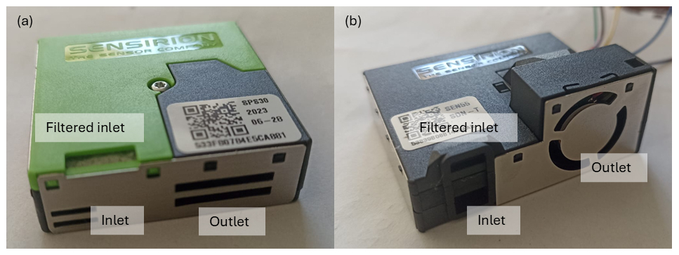
The Sensirion SPS30 is a sensor based on light-scattering (wavelength 660 nm), with one inlet for sample flow and one inlet for filtered sheath air (Fig. A1). Air is drawn into the sensor, where it passes a laser beam and photodiode. Particles in the airstream cause light scattering, which is detected by the photodiode. The detected scatter is used as measurement of mass and number concentrations. The SPS30 reports number concentrations in five bins (upper bin borders of 0.5, 1, 2.5, 4 and 10 µm) and mass concentrations in four particle sizes (PM₁, PM_2.5, PM₄, PM₁₀). As per company specifications, the PM_2.5 measurement range is 0–1000 µg m⁻³, with an uncertainty of $\mathrm{5}\mathrm{\mu }\mathrm{g}{\mathrm{m}}^{-\mathrm{3}}+\mathrm{5}\mathit{\%}$ <100 µg m⁻³, and 10 % at 100–1000 µg m⁻³ (Sensirion, 2023). The sensor can however report much higher values, well over 50 000 µg m⁻³ (Dingemanse, 2022).

The Sensirion SEN55 uses the same measurement technology for PM (light-scatter) and reports the number and mass concentration in the same size bins. Like the SPS30, it has one sample flow inlet and one filtered inlet (Fig. A1). Its measurement range and uncertainty as per company specifications is the same as the SPS30 (Sensirion, 2022). The theoretical maximum value it can report is 6553.4 µg m⁻³, as all output is truncated to a 16-bit unsigned integer with one digit. Apart from the dimensions and the output truncation, the main difference with the SPS30 is that the SEN55 has additional integrated sensor modules for temperature, relative humidity, VOC and NO_x.

Both the SPS30 and SEN55 PM_2.5 mass concentrations are factory calibrated to a TSI DustTrak DRX 8533. The SPS30 PM_2.5 number concentrations are calibrated to a TSI OPS 3330 (Sensirion, 2022, 2023). Calibration is conducted with potassium chloride (Sensirion, 2020).

2.2.2 Reference instruments

For outdoor measurements, filter samples were collected with a Leckel Low Volume Sampler (LVS6-RV; LVS) equipped with a PM_2.5 inlet. The LVS has a continuous flow rate of 2.3 m³ h⁻¹, with which it loads a 47 mm filter. The LVS6-RV is a standard reference sampler according to specifications in CEN EN 12341. In case of power interruption, upon restart of power the LVS automatically continues until the preset sampling time is reached. We tracked moments of power interruption with a power logger.

For indoor measurements, two UPAS V2.0 instruments with PM_2.5 inlet were used. The UPAS has a flow rate of 1 L min⁻¹, with which it loads a 37 mm filter.

The flow rates were validated during the measurement period with a handheld Kytola flow meter (models A-8PR and A-2BR for the LVS and UPAS, respectively). After the measurement period, the flow rates were validated with the TSI Flow Calibrator (model 4048). The LVS and UPAS flow rates were within 5 % of their expected flow rate.

Gravimetric analysis of filters was conducted with a Mettler Toledo AE240, which has a repeatability of 20 µg (Appendix B1). We estimated the LVS and UPAS expanded uncertainty (95 % confidence interval) to be respectively 6.0 % and 12.2 % (Appendix B4).

2.2.3 Relative humidity and temperature measurements

We measured relative humidity (RH) and temperature (T) with the SEN55, which has rated accuracies of ±4.5 % and 0.45 °C for RH and T, respectively (Sensirion, 2022). To verify these accuracies, we compared the SEN55 data to a collocated thermohygrograph (THG), finding correlations ≥0.96 (Appendix C1.1). The SEN55 exhibited a temperature offset that propagated into an RH offset. Since this offset is likely due to self-heating (Appendix C1.3), we assumed that the SEN55 RH and T are the best indication of the corresponding PM measurements.

2.3 Measurements

Across three boxes, six SPS30 (SPS1-6) and six SEN55 (SEN1-6) were used throughout the study. For data logging, the SPS30 and SEN55 sensors were interfaced with a microprocessor, a memory card module, and a clock module (Appendix A1). We placed the sensor systems at a height of 1 to 2.2 m (details in Appendix A2). Table 1 gives an overview of all measurement times.

Table 1 Sensor installation periods and number of gravimetric samples.

For phase 1 and phase 3, measurement frequency of all sensors was set to 1 min. For phase 2, measurement frequency was set to 10 s. Details regarding sensor data management are provided in Appendix A3. Details of gravimetric procedures and an overview of all gravimetric measurements are provided in Appendix B. We discarded eight filter samples (9 % of 85 samples, see Appendix B3).

2.4 Data analysis

We first converted raw sensor into ten-minute averages. Depending on the metric (see Sect. 2.4.1 and 2.4.2), we then used hourly or daily averages for quality evaluation. We included only hour-averages of hours that had a full set of six ten-minute averages, while we included daily averages of days that contained at least 18 h-averages.

2.4.1 Precision

For comparison of identical sensors (precision), we use the coefficient of variation (CV), also called relative standard deviation (Tryner et al., 2020). We calculated the CV with Eq. (1) (Sousan et al., 2016):

$$\begin{array}{}\text{(1)}& \text{CV}={\displaystyle \frac{\mathrm{1}}{n}}\sum {\displaystyle \frac{{\mathit{\sigma }}_i}{{\mathit{\mu }}_i}}.\end{array}$$

Where, σ_i is the standard deviation and μ_i is the mean of measurements of identical sensors during time period i, and n is the number of time periods. The duration of the time period is not prescribed. We use hourly averages since that is a common reporting period for air quality monitors. According to EPA and NIOSH, CV values below 10 % are acceptable (EPA, 2006; NIOSH, 2012).

We additionally use the between-sampler uncertainty (u_bs) as defined in the Guide for Demonstration of Equivalence (GDE) (European Commission, 2010). The u_bs must be calculated with Eq. (2) (European Commission, 2010):

$$\begin{array}{}\text{(2)}& u_{\text{bs}}=\sqrt{{\displaystyle \frac{\sum (y_{i,\mathrm{1}}-y_{i,\mathrm{2}}{)}^{\mathrm{2}}}{\mathrm{2}n}}}.\end{array}$$

Where, y_i,1 and y_i,2 are the results of parallel measurements for time period i, and n is the number of time periods. Time period length should be 24 h. The GDE prescribes to test the u_bs for all data points, as well as for datasets of all values below and above 18 µg m⁻³ separately. There are acceptable u_bs values at two levels: <2.5 µg m⁻³ for fixed reference-grade measurements (European Commission, 2010), and <5 µg m⁻³ for indicative sampling (CSA Group Testing UK Ltd, 2025a). The u_bs is an absolute value, meant for outdoor concentration measurements. With equal relative errors, high concentrations likely lead to absolute errors beyond 2.5 and 5 µg m⁻³. For the calculation of the u_bs we therefore ignored any hours with ten-minute averages beyond 1000 µg m⁻³.

2.4.2 Accuracy

For comparison of sensors with gravimetry measurements, we calculated Pearson's correlation (r), root mean square error (RMSE) and slope (S) and coefficient of determination (R²) from a linear regression model of slope only ($y=S\cdot x$), with gravimetric measurements as y and sensor measurements as x. As linear model, we used weighted least squares (WLS) regression. The regression is weighted with $\frac{\mathrm{1}}{y^{\mathrm{2}}}$ to give data points at low concentration values equal weight with those of high concentration values. Under Appendix D2, we show results of WLS of a model including intercept I ($y=S\cdot x+I$).

We also used accuracy metrics published by the National Institute for Occupational Safety and Health (NIOSH): accuracy error (AE) with accompanying bias (B). We calculated B with Eq. (3) (NIOSH, 2012):

$$\begin{array}{}\text{(3)}& B={\displaystyle \frac{\mathrm{1}}{n}}\sum \left({\displaystyle \frac{x_i}{y_i}}-\mathrm{1}\right).\end{array}$$

Where, x_i is the concentration of the sensor and y_i the concentration of the reference instrument for time period i, and n is the number of time periods. When B is larger than |10 %|, corrected data x_new must be calculated based on old data x_old with Eq. (4) (NIOSH, 2012):

$$\begin{array}{}\text{(4)}& x_{\text{new}}={\displaystyle \frac{x_{\text{old}}}{B+\mathrm{1}}}.\end{array}$$

The AE is the maximum difference between $\frac{x_i}{y_i}$, as percentage of y_i, at a 0.95 probability (NIOSH, 2012). We calculated the AE as the upper value of the confidence interval at 90 % of all values $\frac{x_i}{y_i}$. Acceptable values for AE are <25 % (NIOSH, 2012).

For outdoor conditions, we additionally use the expanded uncertainty (W_CM) as defined in the GDE. The W_CM should be tested both for the whole dataset, as well as a dataset of values >18 µg m⁻³. For the W_CM, a linear relationship between sensor and reference measurements is assumed. For this linear relationship, algorithms of orthogonal regression (OR) should be used. If slopes are significantly different from 1, and/or the intercept is significantly different from 0, data should be corrected for this. We conducted regression calculations and determinations of slope and intercept significance according to the equations shown in the GDE (GDE Sect. 9.5 and GDE Appendix B). Part of these calculations include a correction for the uncertainty of the reference method. We used 0.9 µg m⁻³ for this (see Appendix B4). There are acceptable W_CM values at two levels: for fixed reference-grade measurements <25 %, while for indicative sampling <50 % (European Union, 2015).

All presented post-correction values are based on the same observations used to establish those corrections. This approach is similar to for example MCERTS certification, where instruments can be certified using data after applying a correction derived from that same dataset.

2.4.3 High-concentration evaluation

We investigated how high particle loads affect sensor operation by checking precision during low-concentration hours (average <50 µg m⁻³), within one or two hours after an hour that contained a high concentration measurement (>1000 µg m⁻³).

We also tested the validity of data at the SEN55's digital truncation limit (6553.4 µg m⁻³, see Sect. 2.2.1). A Pearson Chi-square test was performed on two SEN55/SPS30 pairs to see if the maximum value occurrences matched significantly at both 10 min and hourly resolutions. To measure the impact of truncation, we compared the SEN55 to SPS30 correlation slopes of the complete dataset against a version excluding these maximum values. Finally, we compared five data handling strategies for high concentrations: (1) the full, untruncated dataset, (2) values >6553.4 µg m⁻³ truncated to that value (SEN55 logic), (3) values >6553.4 µg m⁻³ removed as errors, (4) data points beyond 1000 µg m⁻³ truncated to 1000 µg m⁻³ (manufacturer specification interpretation), or (5) values >1000 µg m⁻³ removed.

2.4.4 Effect of relative humidity

To check whether the SEN55 and SPS30 are affected similarly by relative humidity, we evaluated the SEN55 to SPS30 ratio across relative humidity levels.

To check for a possible hygroscopic effect, we evaluated the SEN55 to gravimetry ratio for different relative humidity bin-sizes. We did this for both the original SEN55 data, as well as SEN55 data corrected for a theoretical hygroscopic growth. We used the κ-Köhler theory to calculate the theoretical growth factor of the mass based on the relative humidity GF(RH), with Eq. (5) (Blaga, 2024; Crilley et al., 2018; Petters and Kreidenweis, 2007):

$$\begin{array}{}\text{(5)}& \text{GF}\left(\text{RH}\right)=\mathrm{1}+\mathit{\kappa }\cdot {\displaystyle \frac{\text{RH}}{\frac{{\mathit{\rho }}_{\text{particle}}}{{\mathit{\rho }}_{\text{water}}}\cdot (\mathrm{100}-\text{RH})}}.\end{array}$$

The density of water ρ_water is 1 g cm⁻³, and we used 1.65 g cm⁻³ as bulk dry particle density ρ_particle (Crilley et al., 2018). κ is a constant representing the hygroscopicity of the particles. There is high variation in hygroscopicity per particle (and the related complexity in one κ-value for particle mixtures). We could also find no studies on hygroscopicity of the Ethiopian urban and rural environment. We therefore use a κ-value suggested for continental aerosols in general: 0.3 (Andreae and Rosenfeld, 2008). We additionally show the results with a κ-value representing lower hygroscopicity (0.19), since biomass burning is part of the sources and specifically for biomass burning typically lower hygroscopicities are found (Kreidenweis and Asa-Awuku, 2014).

We only evaluate relative humidity effects for phase 1 and 3 data. The phase 2 measurements had a low relative humidity variation (40 %–60 %) with extreme concentration events, hence biasing the analysis at a limited range of relative humidity.

3 Results

3.1 Concentration levels

This section shows the conditions of our measurements. We present the concentration levels measured in the three phases (Sect. 3.1.1–3.1.3), as well as the temperature and relative humidity during the measurement period (Sect. 3.1.4).

3.1.1 Phase 1 measurements

Figure 1 shows the concentrations measured at locations Outdoor 1 and 2.

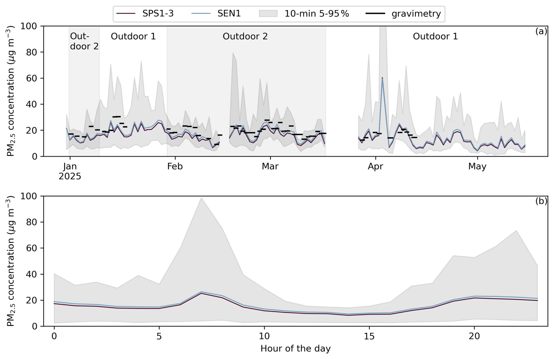
Figure 1 Gravimetry measurements, sensor daily averages (a) and sensor averages per hour of the day (b), as well as 5 %–95 % of 10 min averages, at locations Outdoor 1 and 2. Concentrations in panel (b) are from all days across both locations.

Daily averages at Outdoor 1 and 2 on average were 14.8 µg m⁻³ (min–max 4–33 µg m⁻³). Ten-minute averaged concentrations reached over 80 µg m⁻³. There is a diurnal pattern with elevated concentrations in the morning (06:00–09:00 LT) and evening (18:00–22:00 LT). The morning and evening peaks result from traffic and cooking activities.

3.1.2 Phase 2 measurements

Figure 2 shows concentrations measured in the two kitchens.

Figure 2 PM_2.5 gravimetric measurements, hourly averages and 5 %–95 % 10 min averages at Kitchen 1 (a) and Kitchen 2 (b). The top panel y-scale is limited to 3000 µg m⁻³ for visibility; only on 13 June the 95 % of 10 min averages was beyond 3000 µg m⁻³ (up to 10 000 µg m⁻³).

Concentrations at both kitchens were significantly higher than outdoor concentrations. At Kitchen 1, hourly averages regularly reached up to 1000 µg m⁻³, while at Kitchen 2 they regularly reached up to 4000 µg m⁻³. The gravimetric measurements are an indication of longer-term averages: 100–400 µg m⁻³ at Kitchen 1 and 500–2000 µg m⁻³ at Kitchen 2.

3.1.3 Phase 3 measurements

Figure 3 shows the concentrations measured at location Residence.

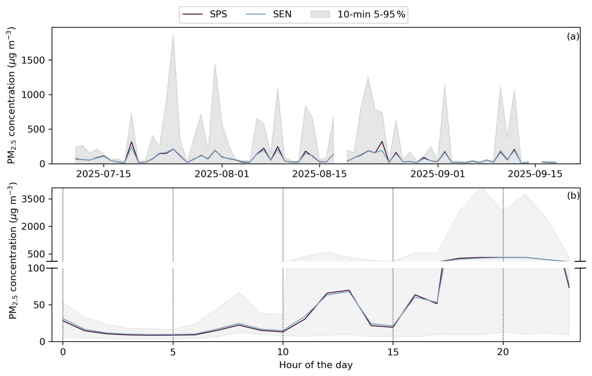
Figure 3 PM_2.5 daily averages (a) and averages per hour of the day (b), as well as 5 %–95 % of 10 min averages, at location Residence. Panel (b) shows the same data in two linear scales: 0–100 and 100–4000 µg m⁻³.

At location Residence, daily averages were in some cases higher than 200 µg m⁻³. Between 02:00 and 10:00 LT, concentrations at this location were comparable to those at Outdoor 1 and 2. However, in the afternoon and even more in the evening high concentrations were measured. Ten-minute averaged concentrations ranged up to 4000 µg m⁻³ between 18:00 and 22:00 LT.

3.1.4 Temperature and relative humidity

Daily average temperatures (T) ranged from 20 to 32 °C. Relative humidities (RH) were lower in January–March, while hourly relative humidities regularly were > 80 % in March–May. T and RH conditions during precision measurements were representative for normal conditions of Arba Minch, while relative humidities during accuracy measurements were on average lower (Appendix C2).

3.2 Precision

In the following sections, we evaluate the precision of the sensors through the between-sampler uncertainty u_bs (Sect. 3.2.1), the coefficient of variation (Sect. 3.2.2), and the possibility of improving the accuracy through sensor-specific corrections (Sect. 3.2.3).

3.2.1 Between-sampler uncertainty

Table 2 shows the between-sampler uncertainty u_bs, Eq. (2), based on daily averages with at least 18 h of data, for all SPS30 and SEN55 sensor pairs, as well as two SPS30 to SEN55 pairs.

Table 2 u_bs for collocated sensor pairs across the study locations. We calculated the u_bs based on all 24 h averages, and separately on those below and those above 18 µg m⁻³ PM_2.5 (see Sect. 2.4.1).

^* For comparing SEN55 to SPS30 sensors, we selected two SEN55 sensors that were installed in systems together with SPS30 sensors (see Appendix A2).

For both the SPS30 and the SEN55, all u_bs values are lower than the GDE requirement of 2.5 µg m⁻³ for fixed reference-grade measurements. This is the case for both datasets of values below and above 18 µg m⁻³. At higher concentrations, with a similar relative error, the error becomes bigger, hence in all cases the u_bs is higher for the datasets with higher concentrations.

The difference between SPS30 and SEN55 instruments is larger than between identical sensor types. Comparing SPS30 to SEN55 pairs results in between-sampler uncertainties of 1.0–3.0 µg m⁻³. This is below the MCERTS threshold for indicative sensors (5 µg m⁻³), but not below that of 2.5 µg m⁻³ for fix reference-grade measurements (GDE). This is especially due to measurements under higher concentrations: the highest u_bs is 3 µg m⁻³, while that of lower values is 1.14 µg m⁻³. Also, the SPS6 to SEN6 comparison results in higher u_bs values than those for SPS1 to SEN1, because we used SPS6 and SEN6 only during the high-concentration phases (2 and 3).

3.2.2 Coefficient of variation

Table 3 shows the CV, Eq. (1), based on 1 h averaged data, for all SPS30 and SEN55 sensor pairs and two SPS30 to SEN55 pairs, for both the whole dataset as well as three concentration ranges.

Table 3 Number of data points (N) and CV for collocated sensor pairs across the study locations. The CV is calculated based on all hour-averages, and separately for the ranges 0–100, 100–1000 and >1000 µg m⁻³.

^* For comparing SEN55 to SPS30 sensors, we selected two SEN55 sensors that were installed in systems together with SPS30 sensors (see Appendix A2).

For all SPS30 and SEN55 sensor pairs, the CV is lower than the threshold for acceptable values set by EPA and NIOSH (10 %). This holds for datasets of all concentration levels, including those beyond the range specified by the manufacturer (>1000 µg m⁻³). It also holds for SPS30 to SEN55 pairs.

3.2.3 Reducing variation

While the precision results of both the SPS30 and the SEN55 are below GDE, NIOSH and EPA thresholds, we can see whether the values can be lowered by distinguishing between random and continuous variations between sensor pairs. Table 4 shows the mean sensor 1 to sensor 2 ratio, and the u_bs and CV after correcting for this ratio.

Table 4 Average ratios (sensor 1/sensor 2), and u_bs and CV for collocated sensor pairs across the study locations after correcting for the average ratios.

^a The average ratio is calculated based on ten random selections by NumPy's random number generator of 30 % of the data. ^b For comparing SEN55 to SPS30 sensors, we selected two SEN55 sensors that were installed in systems together with SPS30 sensors (see Appendix A2).

After correcting for the average ratios, the u_bs and CV are in most cases reduced. Part of the difference between individual pairs is not random, but with a continuous direction. This implies that the accuracy of individual sensors can be improved if users can collocate them to establish individual sensor corrections.

For the SPS30 to SEN55 the average ratio is lower than the ratios between identical sensors (0.89–0.9, while 0.96–1.05 for identical sensors). The correction therefore has a larger effect. For uncorrected values we saw clearly higher CV and u_bs values for SPS30 to SEN55, but with correction they are in the same range as those of identical sensor type pairings. There is one notable exception: the correction does not lead to a decrease of the CV under >1000 µg m⁻³ averages (9.3 % after correction versus 8.7 % before correction). In Sect. 3.4 we will show that a separate high-concentration effect nulls the SEN55 to SPS30 ratio that is otherwise observed.

3.3 Accuracy

We present results on the sensor accuracies in comparison with gravimetric measurements subsequently for outdoor measurements (Sect. 3.3.1) and indoor measurements (Sect. 3.3.2).

3.3.1 Outdoor concentration levels

We show scatter plots of sensor versus gravimetry PM_2.5 outdoor concentrations in Fig. D2. Table 5 shows all quality metrics for comparison of sensor average values with filter measurements of the LVS under outdoor concentration levels.

Table 5 Quality metrics under outdoor conditions for PM_2.5 sensor measurements (per ID) in comparison to gravimetric measurements: number of pairings (N), Pearson correlation (r), Weighted Least Squares (WLS) slope (S) with 95 % confidence interval (CI) and R², root mean square error (RMSE, before→after correction for S), bias (B) and AE before→after correction for B, orthogonal regression (OR) significant correction (sign. corr.) and expanded uncertainty (W_CM) before→after this correction.

^a For WLS, a model with slope only is shown here. Under Appendix D2 we show results for a linear model with intercept. ^b For calculation of the W_CM, correction for slopes significantly different from one and/or intercepts significantly different from zero is required (see Sect. 2.4.2). In all cases, there were significant slopes only.

All sensors require a positive correction as they all reported lower values than the gravimetric measurements. The SPS30 sensors have slopes between 1.19 and 1.23 (significantly different from 1), while the SEN55 has a slope of 1.11 (significantly different from 1). After this correction, the accuracy errors and expanded uncertainties are all lower than the NIOSH and GDE thresholds of 25 % (10 %–12 %). The W_CM for all concentrations beyond 18 µg m⁻³ is in the same order of magnitude: between 12 % and 15 %. The 95 % confidence interval of the SEN55 slope reaches up to 1.14, while those of the SPS30 slopes start from 1.15. The slopes are significantly different from each other; the SEN55 is measuring significantly higher than the SPS30. This corresponds with the finding under Sect. 3.2 that a direct SPS30 to SEN55 comparison revealed bigger differences than those amongst identical sensor types.

When we apply the average correction factor for the SPS30 (1.21) to the SEN55 data, direct comparison with gravimetry results in an RMSE of 2.7 µg m⁻³, an AE of 12.7 %, and a W_CM of 23 %. While the values increase in comparison to correction for the SEN55-slope, the accuracy errors are still within the criterion set for reference equivalent instruments (<25 %). If one can locally calibrate a SEN55, this is preferred. However, the SPS30 and SEN55 are similar enough to allow for extrapolating data quality results of the SPS30 to the SEN55.

3.3.2 Indoor concentration levels

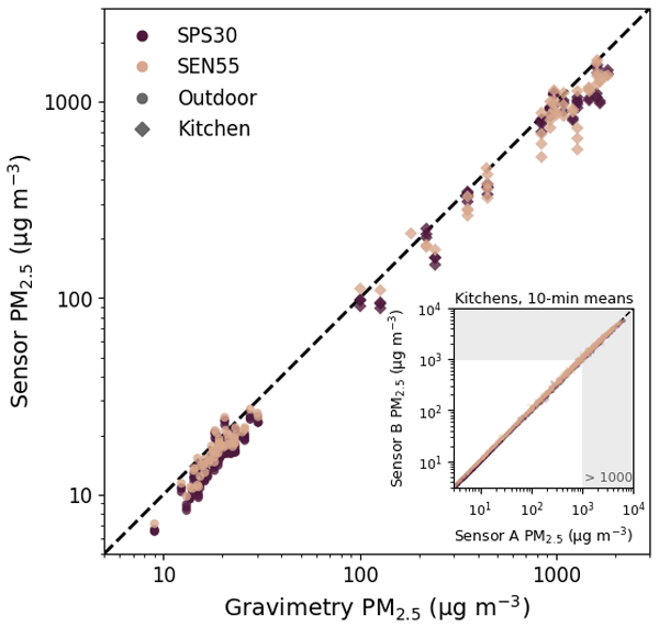
We show scatter plots of sensor versus gravimetry PM_2.5 concentrations in Fig. D3. Table 6 shows all quality metrics for comparison of sensor average values with filter measurements of the UPAS under indoor high-concentration levels.

Table 6 Quality metrics under indoor conditions for sensors (ID) in comparison to gravimetric measurements: number of pairings (N), Pearson correlation (r), Weighted Least Squares (WLS) slope (S) with 95 % confidence interval (CI) and R², root mean square error (RMSE, before→after correction for S), bias (B) and AE before→after correction for B.

^* For WLS, a model with slope only is shown here. Under Appendix D3 we show results for a linear model with intercept.

For all sensors, after correction for an individual bias, the AE is lower than the NIOSH threshold of 25 %. The individual slopes, however, range from 1.07 to 1.19 (SPS30) and 1.01 to 1.25 (SEN55). The high, highly localized and highly variable concentration patterns under these circumstances are most likely one reason for these slope differences. SEN4 and SEN5 were on the same box (see Appendix A1), and their slope is similar (1.24 to 1.25). This is the same for SPS2 and SPS3 (1.18 and 1.16). This would suggest that under high concentrations from close-by sources, location and orientation of the sensors matters. An exception to this pattern are slopes amongst SPS4-6, which all three were on the same box, but where the SPS4 slope is 1.19 versus 1.07 and 1.10 for SPS5 and SPS6.

The averaged slopes for SPS30 and SEN55 are respectively 1.14 and 1.15. When correcting data of all sensors with a slope of 1.14, accuracy errors for individual sensors range from 15 % to 22 %. In other words: while individual correction factors result in higher data quality, the accuracy error with a same correction factor for all sensors (SPS30 and SEN55 alike) is still within the NIOSH range of acceptable values (<25 %).

3.4 Sensor quality under high concentration conditions

We evaluate the precision after high concentration events (Sect. 3.4.1), the effect of SEN55 digital truncation (Sect. 3.4.2), and the effects of possible options for dealing with high concentration values (Sect. 3.4.3).

3.4.1 Precision after high concentrations

Figure 4 shows, for collocated sensor pairs, all hourly averages of all hours one or two hours after an hour with a measurement beyond 1000 µg m⁻³. All datasets are split in half, chronologically, to evaluate whether there is an effect on the sensor precision over time.

Figure 4 Hourly averages one or two hours after an hour with concentrations beyond 1000 µg m⁻³, split chronologically in two.

For all sensor pairs, the variation across them is below the EPA and NIOSH threshold of 10 %. The CVs of the first and second half of the data do not differ significantly from each other. At location Residence, across two months of almost daily high concentrations in the evening, eight sensors consistently returned to similar low readings under low-concentration conditions (Fig. E1). The precision of the sensors remains equally high, also after multiple high-concentration events.

3.4.2 Behavior at SEN55 digital truncation level

The SEN55 truncates all values beyond 6554.3 µg m⁻³ to that maximum value (see Sect. 2.2.1), while the SPS30 reports higher values. A Pearson Chi-square test based on the hour- and 10 min cutoff occurrences for two SPS30 to SEN55 sensor pairs (SPS4 to SEN3 and SPS6 to SEN6) resulted in all cases in a p-value≪0.001 (Appendix E2). The SEN55 cutoff-values are significantly matched to SPS30 values beyond the cutoff.

The extent of this effect fully depends on the number and magnitude of such occurrences. Ordinary least squares regression on hourly averages between the two SPS30 and SEN55 pairs ($\text{SEN55}\cdot \text{slope}=\text{SPS30}$) resulted in slopes of 1.06 and 1.00 for all hourly averages. When ignoring the cutoff occurrences, the slopes become 0.92 and 0.93. For measurements below 6553.4 µg m⁻³, the SPS30 is measuring lower than the SEN55. Measurements beyond the cutoff, however, by definition result in higher values for the SPS30. Under indoor conditions, the higher SEN55 measurements are compensated by the cutoff effect. This is a likely explanation for our finding of similar slopes for SEN55 and SPS30 to gravimetry under indoor conditions (Sect. 3.3.2).

The ratio of SPS30 to SEN55 of 0.92–0.93 for the above pairs' measurements below 6553.4 µg m⁻³ is similar to the ratio in slopes to gravimetry found under outdoor conditions (Sect. 3.3.1; $\mathrm{1.11}/\mathrm{1.21}=\mathrm{0.92}$). The above pairs' measurements are from phase 2 and 3, while the outdoor condition measurements are from phase 1. Also, the outdoor measurements come from other sensor units (SEN1 and SPS1-3 versus here SEN3,6 and SPS4,6). The SEN55 to SPS30 ratio is therefore found in three sensor pairs under two concentration regimes.

3.4.3 Options for dealing with high-concentration values

Data users and sensor system builders can make different choices in dealing with high-concentration values. We distinguish five situations: (1) using all data as is, (2) truncation to 6553.4 µg m⁻³, (3) removal of any value beyond 6553.4 µg m⁻³, (4) truncation to 1000 µg m⁻³, (5) removal of any value beyond 1000 µg m⁻³. Table 7 shows the bias and accuracy errors for sensors in comparison to gravimetry, for these five situations. Scatter plots are shown in Fig. E2.

Table 7 Accuracy error (AE) and bias (B) based on all SPS30 and SEN55 to gravimetry data pairs under indoor conditions, for five situations of dealing with high PM_2.5 concentration values.

The absolute bias increases with the magnitude of truncation or removal, on average from −13 % (situation 1) to −75 % (situation 5). Even without bias correction, for some sensors the accuracy error is below 25 % for both the original data (situation 1) and the data truncated to 6553.4 µg m⁻³ (situation 2). Under situation 2, the absolute bias of the SPS30 is larger than the SEN55, which is further confirmation that the SEN55 measures higher concentrations than the SPS30. When removing all values ≥6553.4 µg m⁻³ (situation 3), for all sensors bias correction is required to have accuracy errors below 25 %. Truncating to 1000 µg m⁻³ or removing these values altogether results in accuracy errors larger than the NIOSH threshold of 25 %. For indoor high-concentration circumstances, measurement values beyond the specified measurement range (1000 µg m⁻³) are required for an accurate representation of the concentration. The fact that accuracy improves upon inclusion of these values, shows that both the SPS30 and the SEN55 can be used under higher concentrations than their specified measurement range.

3.5 Effect of relative humidity

Across eight relative humidity bins of 10 % (12.5 % to 92.5 %), the average SEN55 to SPS30 ratio varied between 1.10 and 1.14 (Fig. F1). There is no significant trend in the SEN55 to SPS30 ratio with an increase in relative humidity. This implies that the SEN55 and SPS30 are affected similarly by relative humidity.

In the SEN55 to gravimetry ratios there are no significant trends with increasing relative humidity (Appendix F2). When correcting SEN55 data with Eq. (5) for GF(RH) with κ=0.3, there is a small but significant negative trend in SEN55 to gravimetry ratios (Appendix F2). A physical correction for hygroscopic growth with assumed average continental hygroscopicity leads to an increasing underestimation with increasing relative humidities. With a lower assumed hygroscopicity (κ=0.19), there is no such underestimation. In both cases, however, corrections were conducted with the SEN55 recorded RH. This RH was significantly lower than ambient RH, likely due to self-heating (Appendix C1). When using ambient RH in the correction, there is a significant overcorrection (underestimation) for both κ=0.3 and κ=0.19.

4 Discussion

4.1 Pragmatic air quality monitoring in Ethiopia

This study compared the performance of two Sensirion low-cost particulate matter sensors – SPS30 and SEN55 – under ambient and indoor conditions in Arba Minch, Ethiopia. The results demonstrate that both sensors achieved high precision, post-correction accuracy, and stability across a wide range of concentrations, with precision and accuracy metrics within relevant criteria for indicative and fixed reference-grade measurements (European Commission, 2010; NIOSH, 2012). Our findings advocate for a pragmatic shift in the “monitoring hierarchy”, particularly for resource-constrained settings like Ethiopia. Traditionally, reference equivalent monitors (REMs) are viewed as inherently superior, yet data does not always support this. For instance, the MCERTS certification of the Palas Fidas 200 showed the requirement of slope correction and expanded uncertainties up to 22.3 % (CSA Group Testing UK Ltd, 2024), while that of the uncorrected SPS30 data for its MCERTS certification ranged up to 8.9 %. Vogt et al. (2021) report for the Palas Fidas a slope and offset of 1.54 and −2.13 versus gravimetry, and a root mean squared error (RMSE) of 2.59 versus for the SPS30 1.92–2.26. Tryner et al. (2020) use the TEOM as reference for the SPS30, but need to apply gravimetric corrections to the TEOM itself. Rabuan et al. (2023) validate the SPS30 with a TOPAS due to the latter being MCERTS certified, but that MCERTS certification is under lower concentrations (<18 µg m⁻³) and with a significantly higher resulting expanded uncertainty (32.2 %) than that of the SPS30 itself (CSA Group Testing UK Ltd, 2025b). These examples highlight that some “reference” instruments introduce errors comparable to the sensors they are meant to validate, making it difficult to justify their high capital and maintenance costs.

In comparison to high-cost REM installations, the high precision and linear response of the SPS30 and SEN55 allow for a more sustainable, locally-managed strategy: deploying such sensors “as-is” and applying calibration factors retrospectively by moving mobile gravimetric units across different regions. Prioritizing long-term OEM sensor stability and simple linear corrections over proprietary “black-box” systems and sparse REM installations ensures that limited budgets expand geographic coverage and provide “higher truth” rather than merely higher-cost data.

4.2 Concentration levels in ambient and indoor environments

The outdoor concentrations in our study (average: 15 µg m⁻³; range: 4–33 µg m⁻³) align with previous ambient SPS30 validation studies, which typically report means between 7 and 35 µg m⁻³ (Dingemanse and Tademe, 2023; Gäbel et al., 2022; Hassani et al., 2023; Hofman et al., 2022b; Hong et al., 2021; Park et al., 2021b). However, this study represents the first extensive SPS30 and SEN55 validation in Ethiopia involving a mixture of traffic, biomass, and open waste burning. Compared to urban centers like Addis Ababa, with reported daily averages up to 80 µg m⁻³, our measured ambient ranges represent the lower end of the Ethiopian urban spectrum (Shlipak et al., 2026; Tefera et al., 2021).

In contrast, indoor validation occurred under high concentrations: gravimetric samples reached 2000 µg m⁻³, with hourly peaks up to 10 000 µg m⁻³. These levels significantly exceed the sensors' specified range. Aside from earlier work in Arba Minch (Dingemanse and Tademe, 2023), few studies have tested the SPS30 or SEN55 under such conditions. We found other indoor validations up to 260 and 500 µg m⁻³ (Penchala et al., 2025; Streuber et al., 2022), and only laboratory studies in a range similar to our study (Findlay et al., 2022: 1400 µg m⁻³; Sousan et al., 2021: 1250 µg m⁻³; Zaid et al., 2023: 3000 µg m⁻³). Despite being “out of range”, these concentrations reflect the reality of Ethiopian households using biomass fuels, where peaks of 3000–4000 µg m⁻³ are common (Admasie et al., 2019; Tamire et al., 2021).

4.3 Precision of SPS30 and SEN55 sensors

Both the SPS30 and SEN55 demonstrated high precision, with results meeting metrics set for reference-grade measurements. The between-sampler uncertainty (u_bs) for the SPS30 (0.23–1.4 µg m⁻³) and SEN55 (1.3–1.5 µg m⁻³) remained well below the European Commision's 2.5 µg m⁻³ threshold (2010). Similarly, the coefficient of variation (CV) for both sensors (1.4 %–5.1 %) was significantly lower than the 10 % limit recommended by the EPA and NIOSH. While some studies have reported higher CVs (e.g., Shittu et al., 2025, at 17.7 %), these are often attributed to single faulty units; our findings align more closely with studies finding u_bs values of 0.3–1.65 µg m⁻³ and CV values <10 % (CSA Group Testing UK Ltd, 2025a; Dingemanse and Tademe, 2023; Hofman et al., 2024; Penchala et al., 2025).

Crucially, this high precision persisted at concentration readings well beyond the sensors' specified range (>1000 µg m⁻³). This reinforces findings from laboratory studies using woodsmoke (Tryner et al., 2020) and coal dust (Zaid et al., 2023), which noted strong R² values (0.94) at concentrations up to 20 000 µg m⁻³. Nguyen et al. (2021) find for smoke under laboratory conditions higher CVs (16.6 %), while Sousan et al. (2021) find a low CV for salt (6.7 %), but 18.7 %–19.7 % for Arizona road dust (ARD) and oil mist. Our study is the first to confirm that this precision holds under real-world Ethiopian conditions for the SPS30 and provides the first documented precision data for the SEN55. Findings of high precision for the SPS30, as referenced by others (Gabriel and Auer, 2023; Mahajan, 2022; Mujan et al., 2021; Park et al., 2021a, b; Riediker, 2022), extents to the conditions of our study, as well as to the SEN55.

Our results demonstrate that precision can be further enhanced by accounting for individual sensor variations. Precision is often viewed as an inherent hardware trait, but factory calibration is a common part of measurement hardware. Factory calibration is fundamentally similar to an additional on-site calibration factor applied by an end-user integrating the OEM sensor into a larger system. Whether a calibration factor is determined by the manufacturer during a final check or by a user during on-site integration, the goal of correcting for sensor-specific variance remains the same.

4.4 Accuracy relative to gravimetric measurements

4.4.1 Outdoor accuracy

Under outdoor conditions, both sensors exhibited strong correlations with gravimetric measurements (r=0.89–0.91, R²=0.99). However, the raw data showed a systematic underestimation of PM_2.5 concentrations, with negative biases of approximately 17 %–20 % for the SPS30 % and 11 % for the SEN55. This resulted in correction factors (slopes) of 1.20–1.24 and 1.12, respectively. Post-correction, accuracy errors (AE; 6.3 %–10.3 %) and expanded uncertainty (W_CM; 8 %–12 %) fell well within the 25 % criterion for fixed reference-grade measurements. In contrast to our findings, some European urban studies report slopes closer to 1.0 and W_CM values of 8.9 % and 12.2 % for uncorrected data (CSA Group Testing UK Ltd, 2025a; Hofman et al., 2022a; Shittu et al., 2025). This discrepancy could stem from factory calibrations performed at higher relative humidities; in our study area's drier climate, reduced hygroscopic growth possibly drives the negative bias. Nevertheless, similar underestimations have been documented elsewhere, including outdoor slopes of 1.09–1.23 in Norway (Vogt et al., 2021), a factor of 1.15 in the Netherlands (Wesseling et al., 2021) and laboratory-confirmed out-of-box bias (Hofman et al., 2024).

4.4.2 Indoor accuracy

Both sensors maintained high linearity under indoor conditions (R²=0.96–0.99), even with concentrations going well beyond the sensor specification range. Average slopes of 1.14 (SPS30) and 1.15 (SEN55) align with a reanalysis of previous findings in Arba Minch (1.13; Appendix G). Notably, the lack of non-linear behavior at these high concentrations argues against instrumental saturation. Following correction, AE values remained below the 25 % threshold. The slightly higher errors found indoors relative to outdoors may be partially attributed to the gravimetric sampler's own uncertainty (UPAS expanded uncertainty estimated at 12.2 %). While Zaid et al. (2023) reported poor SPS30 response to coal dust above 1000 µg m⁻³, our results match the robust linearity found by Sousan et al. (2023) for concentrations up to 15 000 µg m⁻³. The observed indoor slope variations (1.01–1.25) are possibly attributable to local spatial heterogeneity, as some sensor pairs closest to each other exhibited similar slopes. Gaussian plume modelling suggests that a 0.3 m shift from the plume center can imply a 16 % difference in concentration (and from 0.3 to 0.6 m relative to plume center 41 %), a margin consistent with the individual slope variations.

4.4.3 Accuracy and particle composition

Compositional differences likely drive the on average lower slopes (lesser underestimation) observed indoors (1.14) compared to outdoors (1.21). This shift mirrors laboratory findings where the SPS30 reports higher values for wood smoke than for salts or mineral dust (Tryner et al., 2020). However, whereas Tryner et al. reported wood smoke overestimation (slope 0.6) and high variation across aerosols (0.6–2.1), our sensors continued to underestimate concentrations and had a less pronounced slope difference.

The relative stability suggests that real-world Ethiopian biomass emissions differ significantly from laboratory-grade smoke and that the sensors are more consistent under field conditions than controlled experiments might imply. To further isolate the sensor response to real-world biomass fuel particles, future research could either conduct continuous validation against high-resolution reference monitors to assess peak-level performance beyond filter-averaged data, or evaluate performance at lower ambient concentrations in residential areas with high biomass usage to evaluate the influence of aged or diluted smoke.

4.5 Equivalence between SPS30 and SEN55

Direct comparison of collocated SPS30 and SEN55 units revealed high inter-model agreement. Without correction, between-sensor uncertainties (u_bs) were 1.0–3.0 µg m⁻³, within the range for indicative sampling (≤5 µg m⁻³). Under outdoor conditions, a significant difference in slopes was observed (SPS30=1.21; SEN55=1.11). After adjusting for this slope difference, u_bs decreased to 0.41–0.72 µg m⁻³ and the CV dropped from ∼8 % to 3 %–4 %. This demonstrates that the two sensors are functionally equivalent once calibration offsets are accounted for.

The “SEN55-higher” trend persisted across indoor conditions (SPS30$/$SEN55 ratios of 0.92–0.93) and was corroborated by a 0.94 slope found during four months of background measurements in Sweden (Appendix H). While Rodríguez Rama et al. (2024) and Rabuan et al. (2023) similarly noted higher readings from the SEN54/55 compared to the SPS30, our study is the first to quantify these slopes across diverse environments. The SEN55's reduced outdoor underestimation (11 % versus 17 %–20 % for SPS30) suggests a potential factory refinement to the OEM calibration. Provided the systematic ratio between them is recognized, both sensor types are suitable for mixed deployment in monitoring networks, and existing SPS30 performance literature can be extended to the SEN55.

4.6 High-concentration events and sensor stability

Both sensors remained stable and precise following repeated exposures to high concentrations (>1000 µg m⁻³), corroborating laboratory findings by Tryner et al. (2020) where SPS30 precision held after exposures up to 33 000 µg m⁻³. However, a key functional difference emerged: SEN55 measurements are digitally truncated at 6553.4 µg m⁻³, whereas the SPS30 continues to record higher values. Statistical testing (Pearson χ², p≪0.001) confirmed that these SEN55 truncation events corresponded accurately with the SPS30's peak readings, suggesting these peaks are true physical occurrences rather than sensor noise.

Importantly, our results demonstrate that including values beyond the 1000 µg m⁻³ manufacturer specification is essential for maintaining accuracy in high-emission environments; truncating or removing data at that limit would result in unacceptably large accuracy errors. The SEN55 digital truncation did not lead to unacceptable accuracy errors, indicating that SEN55 data remain valid for the measurement range of our study. Because our validation included filter averages up to 2000 µg m⁻³ (encompassing even higher instantaneous peaks), the sensors have been tested under conditions that exceed the average concentrations typically reported for biomass-burning environments in Ethiopia (405 µg m⁻³; Enyew et al., 2023), China (85–658 µg m⁻³; Hu et al., 2014), and across Africa (up to 550 µg m⁻³; Safo-Adu et al., 2023). This suggests that both sensors are validated under the range of filter-averaged concentration levels likely to be encountered in real-world biomass fuel indoor air pollution studies.

The robust linear relationship found between filter and sensor averages further suggests that potential high-concentration errors at timeframes smaller than filter-averaged periods are minimal or equally present in both directions. While we cannot verify the accuracy of data at time frequencies below the filter-averaged periods, the consistent reporting of high values at 10 min averaged levels across both sensor types at least indicates these measurements are not random noise, but reactions to physical circumstances. Pragmatically, exposure studies generally prioritize 24 h averages over short-term plumes; our results confirm that for these relevant timescales, the sensors provide a valid and reliable representation.

4.7 Effect of relative humidity

We found no evidence of a relative humidity (RH) effect on the SPS30-to-SEN55 ratio in either Ethiopia or during four months of background monitoring in Sweden (Appendix H). This indicates that both sensors respond to RH similarly. While we found a slight trend between SEN55 and gravimetric measurements relative to RH, applying a correction based on κ-Köhler theory with κ=0.3 resulted in a reversed trend. This implies a slight underestimation by the correction, possibly because the assumed κ-factor is too high for aerosols in our study area. With κ=0.19 we did not find an underestimation. Similarly, no underestimation was observed when applying κ-Köhler correction to background measurements in Sweden (Appendix H). We can find little studies of hygroscopicity over cities with expected similar sources to Arba Minch (biomass fuels, open waste burning). Particles from biomass burning typically exhibit lower hygroscopicity, with studies reporting values between 0.01–0.19 (Kreidenweis and Asa-Awuku, 2014) and specifically 0.06–0.07 for Sub-Saharan the typical Sub-Saharan biomass fuels eucalyptus and cow dung (Mouton et al., 2023). Rissler et al. (2010) suggest a slightly lower value (0.26) for biomass burning regions. Over Cairo (Egypt), Christodoulou et al. (2024) find for smallest particle sizes (dry mobility diameters of 30 and 60 nm) 60 %–80 % to be particles with low hygroscopicity (κ 0.08–0.11); most likely black carbon and organics originating from traffic and biomass burning. However, amongst the bigger particles (90, 120, 160 nm), mixtures of atmospheric salts (eg. NH₄Cl) with significantly higher hygroscopicity (κ 0.28–0.41) are more present – originating from biomass and waste burning. Haslett et al. (2019) estimate a kappa of 0.22 over West-Africa due to the presence of both black carbon and organics with low hygroscopicity (≤0.1) and inorganic ammonium salts (0.52–0.68). Precursors of those salts, are also released by biomass burning (Andreae, 2019; Tomsche et al., 2023). It might well be that a kappa in the range of 0.15–0.25 is closer to reality of Arba Minch, but we do not know it.

More importantly, we conducted corrections with the SEN55 measured RH, which was lower than RH measured by collocated reference instrumentation, both in our study area (Appendix C1) and in Sweden (Appendix H). A likely partial explanation of lower SEN55 RH measurements is sensor self-heating (Appendix C1.3). Using the ambient RH measurements in the κ-Köhler correction led to a significant overcorrection both for our dataset (Appendix F) and the Swedish dataset (Appendix H), which suggests that internal RH is more representative of the conditions particles experience in the sensor. The sensor self-heating then acts as a drier, reducing the effect of ambient RH on hygroscopic growth. We expect the effect of internal heating we witnessed (<3 °C, lower under higher temperatures) in combination with short residence time to be negligible on enhanced evaporation of other volatile particle components such as volatile organic carbons.

Our results align with literature showing that the SPS30 appears less reactive to ambient RH fluctuations compared to other OEM sensors. For instance, Tryner et al. (2020) found that standard RH corrections led to an underestimation at high RH, while Hassani et al. (2023) observed only a slight mean bias increase (∼1 µg m⁻³) across the 60 %–100 % RH range. Hong et al. (2021) noted that while Plantower and Honeywell sensors showed high fluctuations at increasing RH, the SPS30 bias increased only slightly above 80 %, and Vogt et al. (2021) found that sensor systems with an SPS30 showed lowest dependence on RH changes. These findings are likely due to the use of ambient RH in those studies, where the internal sensor RH – lowered by self-heating – explains the diminished hygroscopic response.

In Arba Minch, daily average RH is generally below 80 % and was consistently under 70 % during our gravimetric sampling. Given the sensor's low sensitivity in this range and the possibly lower hygroscopicity of local biomass particles, we do not expect RH to cause significant accuracy errors in cities with similar climatology. While further research is required to validate performance in Ethiopian regions with higher average relative humidities, the commonality of biomass sources suggests that lower particle hygroscopicity may be a shared characteristic. This is a favorable outcome for Ethiopian monitoring: since reference-grade RH data is scarce, the limited need for complex RH-dependent corrections reduces the resource burden for maintaining accurate data.

5 Conclusions

This study provides the first validation of Sensirion SPS30 and SEN55 sensors against gravimetry under outdoor and indoor conditions in an Ethiopian city. Despite concentrations frequently exceeding manufacturer specifications, both sensors demonstrated high stability and precision (u_bs<1.72 µg m⁻³, CV<7.7 %). After applying site-specific correction factors, the sensors met sampling guidelines for accuracy, with outdoor errors below 11 % and indoor errors below 22 %.

A significant finding is the functional equivalence of the SPS30 and SEN55 once inter-model offsets are addressed. While the SEN55 consistently reports higher values than the SPS30, adjusting for this trend yields nearly identical precision metrics (u_bs<1.3 µg m⁻³; CV<3.1 %). This equivalence holds until the SEN55 reaches its digital truncation limit of 6553.4 µg m⁻³. Critically, we find that measurements exceeding 1000 µg m⁻³ are not random noise but meaningful data; ignoring or truncating values at the 1000 µg m⁻³ threshold leads to unacceptably large accuracy errors and an inability to represent the true exposure concentrations under biomass-burning conditions.

Furthermore, while relative humidity (RH) does influence readings, the effect was low and less pronounced than predicted by standard κ-Köhler with ambient RH, likely due to a combination of lower hygroscopicity of local biomass aerosols and lower sensor-internal than ambient RH. This suggests that in climates similar to Arba Minch, the SPS30 and SEN55 sensors can provide reliable data without the need for complex, resource-heavy RH corrections.

To further refine the use of low-cost sensors in Ethiopia, future research should prioritize:

• Hygroscopicity studies: investigating the specific hygroscopicity of Ethiopian biomass and open waste burning aerosols to better understand RH effects on particle measurements.

• Expanded environmental validation: conducting measurements under higher outdoor background concentrations (e.g., Addis Ababa) and higher RH regimes to establish broader regional correction factors.

• High-resolution monitoring: utilizing higher time-frequency validation under biomass burning conditions to gain deeper insight into the differing correction factors for indoor versus outdoor concentrations.

However, the most critical recommendation is to move from validation to active monitoring. Our results indicate that the SPS30 and SEN55 are already sufficiently precise and stable for large-scale application. In resource-constrained settings, limited budgets are most effectively spent by:

• Starting deployment now: utilizing these sensors immediately to build the high-density networks required to mitigate air pollution, rather than waiting for further refinement.

• Prioritizing mobile gravimetry: investing in mobile gravimetric units for validation across the country, which offers higher accuracy and better value than a few stationary reference-equivalent monitors.

• Local capacity building: instead of importing proprietary “black-box” systems, integrating OEM sensors into locally-built systems to save costs, preserve raw data (avoiding “averaging-away” high peaks), and foster technical self-reliance.

Ultimately, the SPS30 and SEN55 provide a robust, cost-effective path toward understanding the air quality challenges in Ethiopia, provided they are supported by pragmatic validation strategies.

Appendix A: Measurement installations

A1 Sensor systems

Figure A1 shows the SPS30 and SEN55 sensors.

The sensors were all connected to microprocessors (Arduino Mega or EPS32). The following set-ups were used:

• Box 1: three SPS30 and one SEN55, connected to an Arduino Mega, sensors sticking out of the box (SPS1-3, SEN1).

• Box 2: three SPS30 and one SEN55 on one Arduino Mega (SPS4-6, SEN6), and two SEN55 connected to two ESP32 (SEN2, SEN3). The six sensors were placed on a railing in front of the box.

• Box 3: two SEN55 to ESP32 individually (SEN4, SEN5) sensors placed on the top of the box.

Figure A2 shows all sensor systems used in this study.

All microprocessors had an SD module for data storage and DS3231 Real Time Clock. The Arduino Mega clock modules were set manually, while the ESP32 modules retrieved their time from an internet time server.

A2 Location and installation description

Figures A3 through A6 show the installations at all locations. Location Outdoor 2 is technically installed indoor, inside a lab behind an open window. There are no sources inside the lab, except for the occasional resuspension of particulate matter when persons are visiting the lab. At location Outdoor 2, there were a distinct morning and evening peak in the same order of magnitude as at location Outdoor 1 (Fig. D1). We therefore assume that concentrations at Outdoor 2 are from similar sources as at Outdoor 1, and for this reason use data of both locations as one “outdoor” dataset. Additionally, Appendix D2 shows results for the locations separately.

Kitchen 1 and 2 locations both are university campus restaurant kitchens, with therefore regular cooking throughout the day. Kitchen 1 is approximately 12 m×4 m surface area, with multiple cooking places. Kitchen 2 is smaller (approximately 4 m×5 m), with two cooking places. Cooking places are at ground level. Cooking is conducted with wood, with no dedicated ventilation. Both kitchens have only natural ventilation through door openings and space between the wall and the roof (see Figs. A4 and A5).

At location Outdoor 1, the LVS was placed at a height of one meter, and box 1 was placed in a wooden box for weather protection. At Outdoor 2, the LVS and box 1 were placed at similar heights close to windows of the lab. At Kitchen 1 and 2, the sensor boxes and UPAS instruments were placed in a metal cage at a height of 2 m. Horizontal distances between nearest cooking place were three and one meter for Kitchen 1 and 2, respectively. At location Residence, the sensor boxes were placed at the front entrance behind metal mesh with direct communication with the outdoor air, at a height of 2.20 m.

A3 Data management

SPS1 encountered a period of malfunctioning, after which data has been left out. Due to an unreliable battery pack, the microprocessor of SPS1-3 and SEN1 caused spurious results. This data has been left out.

In comparison with gravimetric measurements, phase 2 data of SEN1 and SEN2 are ignored in the main text analysis. SEN1 was positioned perpendicular to all other sensors and gravimetric measurements (Fig. A2). Under high concentrations, sensor orientation affects the measurements (Zaid et al., 2023). Due to power problems SEN2 encountered data loss and was left with only 6 valid pairings. For completeness and additional support for leaving it out, their data is shown under Sect. D.3.

Figure A1 SPS30 (a) and SEN55 (b) sensors.

Figure A2 Overview of three boxes with all SPS30 and SEN55 sensors used across this study.

Figure A3 Sensor and gravimetric instrument installations at locations Outdoor 1 and 2.

Figure A4 Sensor and gravimetric instrument installations at location Kitchen 1.

Figure A5 Sensor and gravimetric instrument installations at location Kitchen 2.

Figure A6 Sensor installations at location Residence.

Appendix B: Gravimetry

B1 Standard deviation of analytical balance

As per the user manual, the readability (standard deviation) of the AE240 analytical balance is 20 µg (IET, n.d.). The analytical balance at the Arba Minch University lab is not included in an official calibration scheme. Instead, with every weighing moment, control weights are weighed along. Since February 2025, three pieces of aluminium foil are used as control weights. Figure B1 shows all weights across 75 weighing moments.

Figure B1 Weight results (n=75) of three control weights, relative to their average weight.

Across 75 weighing moments, the standard deviations for the three control weights are 17, 15 and 21 µg, respectively. We can therefore assume that the standard deviation as provided by the instrument manufacturer is correct, and that the analytical balance operates as expected.

B2 Gravimetric procedures

Standard protocol involved three or more pre- and post-sampling weighings, though 27 filters subject to load-capacity testing received single intermediate weighings. Both dedicated blanks and unused sampling filters were used for correction. During a rainy period at the Outdoor 1 site (27 March–11 April), three sampling filters were repurposed as field blanks to control for humidity-induced weight discrepancies between the field and the laboratory.

To determine the final mass, the differences between all possible pre- and post-sampling weight combinations were calculated and averaged. These values were then corrected using the mean mass change observed in the corresponding blanks.

Based on the standard deviation of the analytical balance (20 µg, see Sect. B.1) and the above calculation, we calculated a theoretical standard deviation SD_T of the PM_2.5 weight with Eq. (B1):

$$\begin{array}{}\text{(B1)}& {\text{SD}}_{\mathrm{T}}=\sqrt{{\text{SD}}_{\text{field}}^{\mathrm{2}}+{\text{SD}}_{\text{blank}}^{\mathrm{2}}},\end{array}$$

where SD_field and SD_blank are calculated with Eqs. (B2) and (B3):

$$\begin{array}{}\text{(B2)}& {\displaystyle }{\text{SD}}_{\text{field}}=\sqrt{{\displaystyle \frac{{\mathrm{20}}^{\mathrm{2}}}{N_{\text{Pre}}}}+{\displaystyle \frac{{\mathrm{20}}^{\mathrm{2}}}{N_{\text{Post}}}}}\text{(B3)}& {\displaystyle }{\text{SD}}_{\text{blanks}}={\displaystyle \frac{\sqrt{\frac{{\mathrm{20}}^{\mathrm{2}}}{N_{\text{pre}}}+\frac{{\mathrm{20}}^{\mathrm{2}}}{N_{\text{post}}}}}{\sqrt{N_{\text{Blanks}}}}}.\end{array}$$

With N_pre and N_post being the number of pre- and post-weighings, and N_Blanks the number of blanks. Table B1 shows an overview of all gravimetry numbers and results.

Table B1 Overview of all gravimetric measurements, with number of pre-weighings (Pre), post-weighings (Post), blanks (B), location, sample period (Start, End), hours of power interruption (PI) during the sample, sampled volume, blank-corrected weight and theoretical standard deviation of the weight (SD_T) across pre- and post-weighing pairings. SD_T is given in µg, and in percentage relative of the total weight.

^* The LVS depends on a power supply, and stops operating during a power interruption. A power logger kept track of moments of power interruption. For filter to sensor comparison, this information was used to select only data from the sensors during which the LVS had been running.

B3 Gravimetry data management

Eight filter measurements were excluded: L21 was removed due to LVS flow instability, L49 was identified as an outlier via Grubb's test at 99 % confidence level, following GDE guidelines (European Commission, 2010), and filters U07-U12 were excluded because their theoretical standard deviation (Eq. B1) exceeded 12.5 % of total mass. The 12.5 % as threshold level was a self-selected compromise between data loss and gravimetric error magnitude.

For sensor-to-filter comparisons, all data points between start- and end-times of filter sampling were used, excluding any periods of LVS power interruption. Sensor averages were only included if they maintained at least 90 % coverage of the 10 min averages during the respective filter sampling period.

B4 Gravimetric instruments uncertainty

According to the Guide for Demonstration of Equivalence (GDE), the maximum allowable uncertainty between two reference instruments such as the LVS is 2 µg m⁻³ (European Commission, 2010). This translates to 1.41 µg m⁻³ for one instrument, at one standard deviation (68 % confidence interval). The GDE expresses expanded uncertainty (uncertainty with a 95 % confidence interval) as percentage relative to a level of 30 µg m⁻³. 1.41 µg m⁻³ translates to 4.7 % uncertainty. The expanded uncertainty (95 % confidence interval) is then 9.4 %. The error of the LVS measurement is most likely lower. We expect the main error components of the gravimetric measurements to be the gravimetry (filter weighing), and the instrument flow rate. For gravimetry with the LVS, the average standard deviation as percentage of filter weight (Table B1) was 2.2 %. Since the LVS is according to CEN EN 12341, the flow uncertainty is lower than 2 % (TUV SUD, 2025). These two main error components give a combined uncertainty of $\sqrt{{\mathrm{2.2}}^{\mathrm{2}}+{\mathrm{2}}^{\mathrm{2}}}=\mathrm{3.0}\mathit{\%}$, implying an expanded uncertainty of 6.0 %. The absolute uncertainty at a level of 30 µg m⁻³ with 3 % is 0.9 µg m⁻³.

For gravimetry with the UPAS, the average standard deviation as percentage of filter weight (Table B1) was 8.8 %. We however excluded filters from the analysis with a standard deviation beyond 12.5 % (see Sect. B.3). Without these filters, the average standard deviation becomes 3.5 %. As per company specification the flow uncertainty is 4 % (Access Sensor Technologies, 2024). This gives a combined uncertainty of $\sqrt{{\mathrm{3.5}}^{\mathrm{2}}+{\mathrm{4}}^{\mathrm{2}}}=\mathrm{6.1}\mathit{\%}$, implying an expanded uncertainty of 12.2 %.

Appendix C: Meteorology

C1 SEN55 RH and T validation

C1.1 Comparison with thermohygrograph

To validate SEN55 measurements of relative humidity (RH) and temperature (T), we collocated a thermohygrograph (THG) with the SEN55 at location Outdoor 1. A THG has an expected accuracy of 3 % and 1 K for RH and T, respectively (World Meteorological Organization, 2008). Figure C1 shows the temperature and relative humidity as measured by the THG and SEN55.

Figure C1 Temperature and relative humidity as measured by the thermohygrograph (THG) and SEN55. For the SEN55, corrected values (see Sect. C.1.2) are also shown.

At the same location, the daily averages of the SEN55 closely matched those measured by the THG (RMSE of daily averages for T and RH 1.5 °C and 7.1 %, r of 0.96 and 0.97, respectively).

C1.2 Offset and slope of SEN55

The SEN55 relative to the THG measures higher temperatures and lower relative humidities (Fig. C1). We expect that the RH error is a direct (physical) result from the T error. This implies that based on a statistical temperature correction, RH can be corrected based on physical relations.

The Clausius-Clapeyron derivative substituted into an RH change to temperature change relation gives Eq. (C1):

$$\begin{array}{}\text{(C1)}& {\displaystyle \frac{\mathit{\delta }\text{RH}}{\text{RH}}}\approx -{\displaystyle \frac{L_{\mathrm{v}}}{R_{\mathrm{v}}{T}^{\mathrm{2}}}}\mathit{\delta }T.\end{array}$$

In which L_v is the latent heat of vaporization (approximately 2.5×10⁶ J kg⁻¹ in our temperature range with a molar mass of 18.015 g mol⁻¹) and R_v is the specific gas constant (461 $\mathrm{J}{\mathrm{kg}}^{-\mathrm{1}}{\mathrm{K}}^{-\mathrm{1}}$). In our temperature range of 288–308 K, $\frac{L_{\mathrm{v}}}{R_{\mathrm{v}}{T}^{\mathrm{2}}}$ varies from 0.057 to 0.065. We therefore rewrite to Eq. (C2):

$$\begin{array}{}\text{(C2)}& \mathrm{\Delta }\text{RH}\approx -\mathrm{0.06}\cdot \text{RH}\cdot \mathrm{\Delta }T.\end{array}$$

With ΔT being T_SEN55−T_real.

We can rewrite to calculate RH_corrected based on T_SEN55, RH_SEN55 and an estimated T_real with Eq. (C3):

$$\begin{array}{}\text{(C3)}& \begin{array}{rl}{\text{RH}}_{\text{corrected}}& \approx {\text{RH}}_{\text{SEN55}}\\ & +\mathrm{0.06}\cdot {\text{RH}}_{\text{SEN55}}\cdot (T_{\text{SEN55}}-T_{\text{real}}).\end{array}\end{array}$$

We estimate T_real based on ordinary least squares (OLS) regression between T_SEN55 and T_THG. This resulted in a slope of 1.27 and intercept of −8.0 (R²=0.85). In other words, we calculated T_real with Eq. (C4):

$$\begin{array}{}\text{(C4)}& T_{\text{real}}=\mathrm{1.27}\cdot T_{\text{SEN55}}-\mathrm{8.0}.\end{array}$$

Figure C1 shows the corrected SEN55 data. With the corrected RH, the RMSE to RH_THG becomes 2.9 %. For the corrected T this is 0.62 °C. This is well within the compounded accuracy of the SEN55 specified and THG expected accuracies. Given that the physical RH correction resolves the RH error, RH seems accurately measured and the deviation from ambient is due to instrument heating.

C1.3 Reasons for temperature offset

The significant slope and intercept of 1.27 and −8.0 (Eq. C4) indicate that the SEN55 overestimates temperatures, which becomes more pronounced at lower ambient temperatures (as illustrated in Fig. C1). Figure C2 shows the hourly temperature differences (SEN55−THG).

Figure C2 Boxplots of hourly temperature differences between the SEN55 and THG measurements (SEN55−THG).

The hourly temperature difference shows a diurnal pattern (Fig. C2): the average error peaks during nighttime, coinciding with lower ambient temperatures and reduced ventilation, while the error decreases during daytime, approaching zero around 17:00 as environmental temperatures rise and air exchange likely increases. This behaviour is consistent with internal heat dissipation or self-heating. The relative impact of a sensor's internal heat becomes more significant when the gradient between sensor and environment is high and convective cooling (ventilation) is low. We therefore conclude that self-heating is a contributing factor to the observed temperature differences.

Because the SEN55 measures particles under these self-heated conditions, the internal RH is lower than the external ambient RH. Therefore, the RH reported by the SEN55 is the more accurate predictor for hygroscopic growth occurring inside the sensor's measurement chamber.

C2 Representativeness of meteorological conditions

Under outdoor conditions, measurements for precision were conducted between 31 December 2024 and 19 September 2025. Outdoor filter measurements were conducted between 13 April 2025 and 31 December 2024. Figure C3 shows daily and hourly averaged RH and T measured at location Outdoor 1 for a full year (25 December 2024–25 December 2025), and boxplots of hourly averages for the full year, precision measurement and filter measurement periods. The measurements are taken from two other sensors with BME280 relative humidity and temperature sensor. Since we focus here only on the values on average during the different periods (rather than the absolute values), we do not present validation data of the BME280.

Figure C3 Temperature (T) and relative humidity (RH) for a full year (a), and boxplots of hourly values of RH (b) and T (c). The boxplots show values of the full year, of only those during precision measurements, and only those during filter measurements.

The full year average relative humidity and temperature were respectively 47 % and 27 °C. During precision measurements, this was respectively 50 % and 26 °C, while during filter measurements this was respectively 35 % and 28 °C. On average, filter measurements have been under warmer and dryer conditions. During filter measurements, however, there have also been more humid moments: hourly averages ranged up to 80 %.

Appendix D: Gravimetry and sensor measurements

D1 Phase 1 comparison of two locations

Figure D1 shows the daily trend for SEN1 phase 1 measurements of the two locations (Outdoor 1 and Outdoor 2), as well as boxplots of hourly averages.

Figure D1 SEN1 PM_2.5 measurements at locations Outdoor 1 and 2 per hour of the day (a), and boxplots of hourly averages (b). For Outdoor 1, six of the total 1523 hourly averages were higher than 100 µg m⁻³.

Phase 1 measured concentrations of Outdoor 1 and 2 were in the same order of magnitude. The higher variability observed at Outdoor 1 compared to Outdoor 2 can be attributed to the outdoor measurement setting at Outdoor 1, which allows for a more immediate response to environmental changes. We do however assume that particle compositions and concentrations at both locations are comparable enough to use all phase 1 data together in the main text. Under Sect. D.2 we nonetheless show results for the locations separately.

D2 Outdoor sensor versus gravimetry measurements

Figure D2 shows all outdoor sensor versus gravimetry measurements. Table D1 shows results of WLS regression with intercept for these measurements.

Figure D2 Sensor versus gravimetry PM_2.5 concentrations under outdoor conditions, color-grouped by location.

Figure D3 Sensor versus gravimetry PM_2.5 concentrations under indoor conditions.

Table D1 Quality metrics under outdoor conditions for PM_2.5 sensor measurements (per ID) in comparison to gravimetric measurements: Weighted Least Squares (WLS) slope (S) and intercept (I) with 95 % confidence interval (CI) and R², and root mean square error (RMSE) after correction for S and I.

The RMSE for correction with slope and intercept has a slight improvement (slope only: 2.1–2.3; slope and intercept: 1.9–2.1). Given however that orthogonal regression gives only significant slopes (see Table 5), that the NIOSH accuracy error only accounts for a possible bias similar to a slope, and that a slope-only correction is physically more plausible (assuming the reference is the truth, a positive intercept implies that the sensors never measure below 3.5 µg m⁻³, but this is not the case), in our main analysis we present WLS with slope only.

Table D2 shows results of WLS regression without intercept for locations Outdoor 1 and 2.

Table D2 Number of data points (N), Pearson correlation (r) and weighted linear regression (WLS) results for sensor to gravimetry at locations Outdoor 1 and 2 separately. WLS results include slope (S) with 95 % confidence interval (CI) and R², and root mean square error (RMSE, before→after correction for S).

Table D3 Quality metrics under indoor conditions for PM_2.5 sensor measurements (per ID) in comparison to gravimetric measurements: Weighted Least Squares (WLS) slope (S) and intercept (I) with 95 % confidence interval (CI) and R², and root mean square error (RMSE) after correction for S and I.

Table D4 Quality metrics under indoor conditions for sensors (ID) excluded from the main text analysis, in comparison to gravimetric measurements: number of pairings (N), Pearson correlation (r), Weighted Least Squares (WLS) slope (S) with 95 % confidence interval (CI) and R², root mean square error (RMSE, before→after correction for S), bias (B) and AE before→after correction for B.

Regression slopes for Outdoor 1 and 2 do not differ significantly from each other (confidence intervals overlap across the locations for each sensor, Table D2). When applying slopes based on the pooled location data as correction factors to the sensor data (1.23, 1.21, 1.20 and 1.12 for SPS1, SPS2, SPS3 and SEN1, respectively; see Table 5), maximum post-correction AE and W_CM are respectively 16 % and 22 % for Outdoor 1 and 10 % and 11 % for Outdoor 2. In other words, there is no evidence for a significant difference between Outdoor 1 and 2, and using pooled data results does not lead to unacceptable accuracy errors for either location.

D3 Indoor sensor versus gravimetry measurements

Figure D3 shows all indoor sensor versus gravimetry measurements, including those for the discarded SEN1 and SEN2 data. Table D3 shows results of WLS regression with intercept for non-discarded measurements.

In all cases, the 95 % CI of the intercept includes 0. The average RMSE after correction with slope only is 151 and 133 µg m⁻³ for SPS30 and SEN55 respectively, which is relatively close to the RMSE after correction with slope and intercept (146 and 143 µg m⁻³). Additionally, given that the NIOSH accuracy error only accounts for a possible bias similar to a slope, and that a slope-only correction is physically more plausible, in our main analysis we present WLS with slope only.

SEN1 and SEN2 data are excluded from analysis in the main text. Table D4 shows the quality metrics for their data.

SEN1 shows an overall wide variation (Fig. D3), leading to a low r (0.53) and an RMSE significantly higher than any of the other sensors (471 µg m⁻³ versus <254 µg m⁻³ post-correction). SEN1, as part of Box1, was the only sensor positioned perpendicular rather than front-facing, and has been repositioned relative to source and collocated UPAS across the measurement period. SEN2 is quite linear (r=0.91) and closely follows SEN3 (which was positioned with SEN2 on Box 2), but has little data points (n=6). Accuracy errors for both SEN1 and SEN2 are beyond the threshold of 25 %. Given that SEN1 and SEN2 errors are connected to reasons other than sensor quality, we find it valid to leave them out of the main text analysis.

Appendix E: High value sensitivity analysis

E1 Precision around high concentration measurements

At location Residence there were regular high-concentration events in the evenings. In the night-time, concentration became low again. Figure E1 shows for three weeks across the location's measurement period the concentration, with those night-time concentrations highlighted.

Figure E1 Hourly average concentration for eight sensors at location Residence, three weeks across the measurement period. Measurements between 02:00–06:00 are highlighted, and y-axis limits are optimized for those concentrations only.

Across the whole measurement period, after high-concentration events eight sensors measured similar concentrations. The sensors could still register low concentrations with high precision.

E2 Cutoff occurrences

The SEN55 truncates all values beyond 6553.4 µg m⁻³ to that maximum value (see Sect. 2.2.1), while the SPS30 reports higher values. Table E1 shows the number of data periods that had or had not one or more of these maximum measurements, for two sensor pairs: SPS4 with SEN3 and SPS6 with SEN6.

Table E1 Contingency tables of occurrences beyond and below the SEN55 PM_2.5 cut-off, for two SPS30/SEN55 sensor pairs, for hourly and 10 min periods. Data periods that contain raw data with at least one value ≥6553.4 µg m⁻³ are classified as beyond the cut-off.

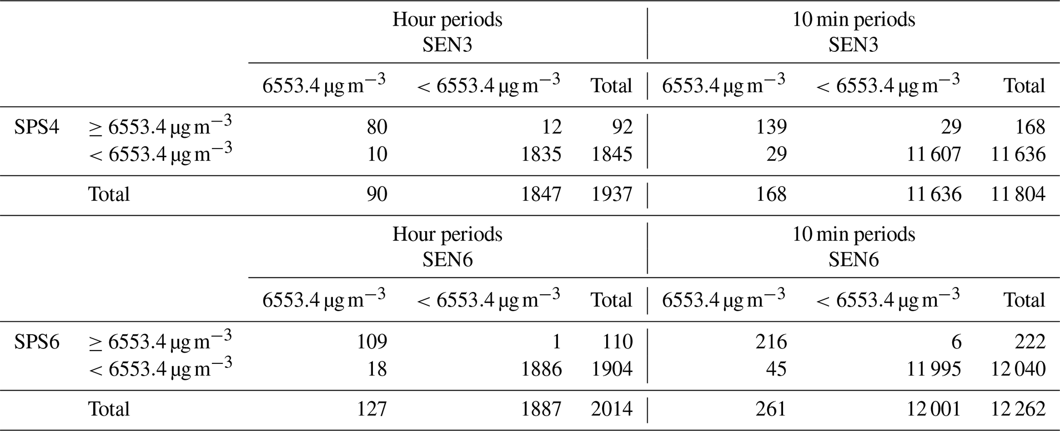
The SPS4 and SPS6 measured beyond 6553.4 µg m⁻³ during respectively 92 and 110 h, and during respectively 168 and 222 10 min periods. Of these, during respectively 80 and 109 h and 139 and 216 10 min periods the collocated SEN55 registered cut-off values. A Pearson Chi-square test based on the hour- and 10 min occurrences as shown in Table E1 resulted in all cases in a p-value≪0.001. The SEN55 cutoff-values are significantly matched to SPS30 beyond the cutoff.

E3 Effect of concentration cutoff

Figure E2 shows scatter plots for sensors versus gravimetry measurements, for five situations of dealing with high sensor values: no cut-off (S1), truncation to 6553.4 µg m⁻³ (S2), removal beyond 6553.4 µg m⁻³ (S3), truncation to 1000 µg m⁻³ (S4) and removal beyond 1000 µg m⁻³ (S5). While sensor to gravimetric measurements without cut-off are linear, truncation or removal of high-concentration measurements leads to an increasing underestimation.

Figure E2 Sensor to gravimetry comparison for five situations (S1 through S5 in panels a through e, see Sect. 3.4.3 for details), for any SPS30 (SPS) and SEN55 (SEN).

Appendix F: Relative humidity

F1 SEN55 to SPS30 ratio under RH changes

Figure F1 shows the ratio of SEN55 to SPS30 ten-minute averages, categorized in 10 % relative humidity bins.

Figure F1 SEN55 to SPS30 ratios of ten-minute averages. The boxes show 25 % to 75 % percentiles of the data (Q1 and Q3). The whiskers extent to $\mathrm{1.5}\cdot (\text{Q3}-\text{Q1})$ below Q1 and above Q3.

The average of all ratios per RH bin size varies between 1.10 and 1.14, and there is no significant trend in the ratios. An Ordinary Least Squares (OLS) regression model with $\frac{\text{SEN55}}{\text{SPS30}}=\text{RH}\cdot \text{slope}+\text{intercept}$ gives a non-significant slope (p=0.699). There is no evidence that the SEN55 to SPS30 ratio is affected by RH, and we can therefore assume that any effect from RH for the SEN55 is similar for the SPS30.

F2 Effect of hygroscopic growth

With Eq. (5) we can calculate expected growth factors based on relative humidity GF(RH). If the SEN55 measurement data is affected by hygroscopic growth as predicted by the κ-Köhler theory, we should see an increase relative to gravimetric measurements with increasing relative humidity, and no such increase when dividing the data points by their respective growth factors. Figure F2 shows the absolute and relative SEN55 to gravimetry differences (with averages per 10 % relative humidity bin), for both uncorrected and GF-corrected data with κ=0.3. Table F1 shows trends and corresponding p-values, for both κ=0.3 and κ=0.19. We present GF-corrected data both with correction based on SEN55 RH, and RH representative for ambient RH.

Figure F2 Differences between SEN55 and gravimetry measurements: absolute (SEN55−gravimetry) and relative ($(\text{SEN55}-\text{gravimetry})/\text{gravimetry}$), for uncorrected values (a, b), GF-corrected values (c, d), and GF-corrected values based on RH corrected with Eq. (C3) (e, f).

Table F1 Slopes, with p-values, of a regression between relative humidity (x) and absolute or relative SEN55 to gravimetry difference (y).

Starting from the 40 %–50 % relative humidity bin, there is a slight upward trend towards higher relative humidities (Fig. F2a and b). Across the whole range, the trend is not significant (p-value of slope for absolute difference to RH is 0.194; for relative difference this is 0.17). With κ=0.3, a correction for GF(RH) results in a slight negative trend for the relative difference (Fig. F2c and d). For the absolute difference after correction there is no significant trend, but for the relative difference the trend is significant (p-value of slope 0.026). Correction for growth factors results in a slight underestimation. When using RH representative for ambient temperatures (Fig. F2e and f), the underestimation becomes more pronounced: a significant negative trend for both the absolute and relative differences (−0.07 µg m⁻³ or −0.005 per % RH, respectively). With κ=0.19, there is no significant trend after correction with the SEN55 reported RH. With ambient RH, the significant trend in the relative difference remains (p=0.02). This supports our statement that the SEN55 reported RH is a better estimator than ambient RH for effects on SEN55 PM_2.5 measurements (see Sect. C.1).

Appendix G: Reanalysis earlier study

In our earlier work, we presented SPS30 and UPAS gravimetry measurements across three kitchens K2–K4 (Dingemanse and Tademe, 2023). Based on these measurements, we presented a slope (from Ordinary Least Squares Regression) of 0.95, a bias (B) of −8 %, and an accuracy error (AE) after bias correction of 13 %. The data file is available at https://osf.io/cezqa (last access: 4 November 2026).

In the current study, we have two changes in our analysis: we assume orientation matters (and therefore only include collocated sensors that are oriented the same as the gravimetric instrument; see Sect. A.3), and we use Weighted Linear Regression (WLS; see Sect. 2.4.2). At kitchen K2, the SPS30 was oriented downward, while the UPAS was placed above it with horizontal orientation. At kitchens K3 and K4, orientation of the SPS30 and UPAS inlets was identical.

Figure G1 shows both the original analysis, as well as OLS for only kitchens K3 and K4, and WLS for kitchens K3 and K4.

Figure G1 Measurements of collocated SPS30 and gravimetric sensors across three kitchens K2–K4 (data from Dingemanse and Tademe, 2023), with regression model lines based on OLS regression of K2 through K4 data, OLS regression of K3 and K4 data, and WLS regression of K3 and K4 data. The legend shows the corresponding slope (S) [with 95 % confidence interval] and the root mean squared error (RMSE) after correction for the slope.

When conducting an analysis identical to our current study, we find a slope of 1.13 between the SPS30 and gravimetric measurements. B and AE after bias correction for only K3 and K4 data are −12 % and 8.5 %, respectively.

Appendix H: Hyltemossa measurements

H1 Measurement installation

Three SPS30 sensors (SPS7–9) and one SEN55 (SEN7) were fixed at the Hyltemossa monitoring site. At that site there is also a Palas Fidas (reference equivalent monitor). For the Palas Fidas (PF) PM_2.5 measurements, expanded uncertainty is 5.7 %–35 % without slope correction, and with 1.06 slope correction it is 8.5 %–22.4 % (CSA Group Testing UK Ltd, 2024). The PF stands free at approximately 10 m from a wooden building. The sensors were installed under a plastic box under the roof extension of that wooden building. Figure H1 shows the installation.

Figure H1 Installation of SPS30 and SEN55 sensors (left) and a Palas Fidas (right) at Hyltemossa monitoring site.

H2 Measurements

Figure H2 shows data measured between 27 May and 12 September 2025.

Figure H2 Hourly average measurements of PM_2.5 and relative humidity (RH) by SPS30 and SEN55 sensors and Palas Fidas (PF) at Hyltemossa.

Apart from an event at 10 June (during which data of the Palas Fidas is missing), concentrations ranged between 0 and 20 µg m⁻³. The relative humidity as reported by the Palas Fidas regularly capped off at 100 %, while that of the SEN55 reported continuously lower values. The lower values can be due to self-heating (see Sect. C.1.3), but are most likely also due to a difference in measurement locations: in the open field for the PF versus next to the building for the SEN55 (see Fig. H1). For evaluating the effects of RH on the PM_2.5 concentrations (Sects. H.3 and H.4), we use the RH as reported by the SEN55, because both self-heating and difference in location imply that the SEN55 RH is the best representation of the RH affecting the sensor measurements.

H2.1 Intra-sensor comparison

Table H1 shows the between-sampler uncertainty (u_bs) and coefficient of variation (CV) for pairs of sensors.

Table H1 u_bs and CV for collocated sensor pairs at Hyltemossa, Sweden.

The three SPS30 have a high precision. The CV based on hourly averages between sensor pairs (Eq. 1) ranges from 1.5 % to 3.2 %. The between sampler uncertainty (u_bs, Eq. 2) ranges between 0.07 to 0.18 µg m⁻³. This is lower than the GDE, NIOSH and EPA thresholds of 10 % and 2.5 µg m⁻³ for CV and u_bs, respectively.

The SPS30 to SEN55 u_bs and CV are also below these thresholds, but higher than those of SPS30 to SPS30. Ordinary Least Squares (OLS) regression between SEN55 and SPS30 hourly values ($\text{SPS30}=\text{slope}\cdot \text{SEN55}+\text{intercept}$), results in a slope of 0.94 (confidence interval at 95 % 0.93–0.94). The intercept is close to zero (0.03 µg m⁻³). The slope is significantly different from 1. The SEN55 is measuring significantly higher than the SPS30.

H2.2 Sensor to Palas Fidas comparison

Figure H3 shows scatter plots of the PM_2.5 measurements for the sensors versus the Palas Fidas hourly and daily averaged data.

Figure H3 Sensor versus Palas Fidas (PF) comparison at Hyltemossa. The line shows the model prediction resulting from Ordinary Least Squares regression.

Slopes of SPS30 to PF range from 0.92 to 0.98 (reflecting a slight underestimation of the SPS30), while that of the SEN55 is 1.04–1.06 (a slight overestimation). The difference in slopes result from the SEN55 measuring higher than the SPS30.

H3 The effect of relative humidity on SEN55 to SPS30 ratio

Figure H4 shows the ratio of SEN55$/$SPS30 ten-minute averages, categorized in 10 % relative humidity bins.

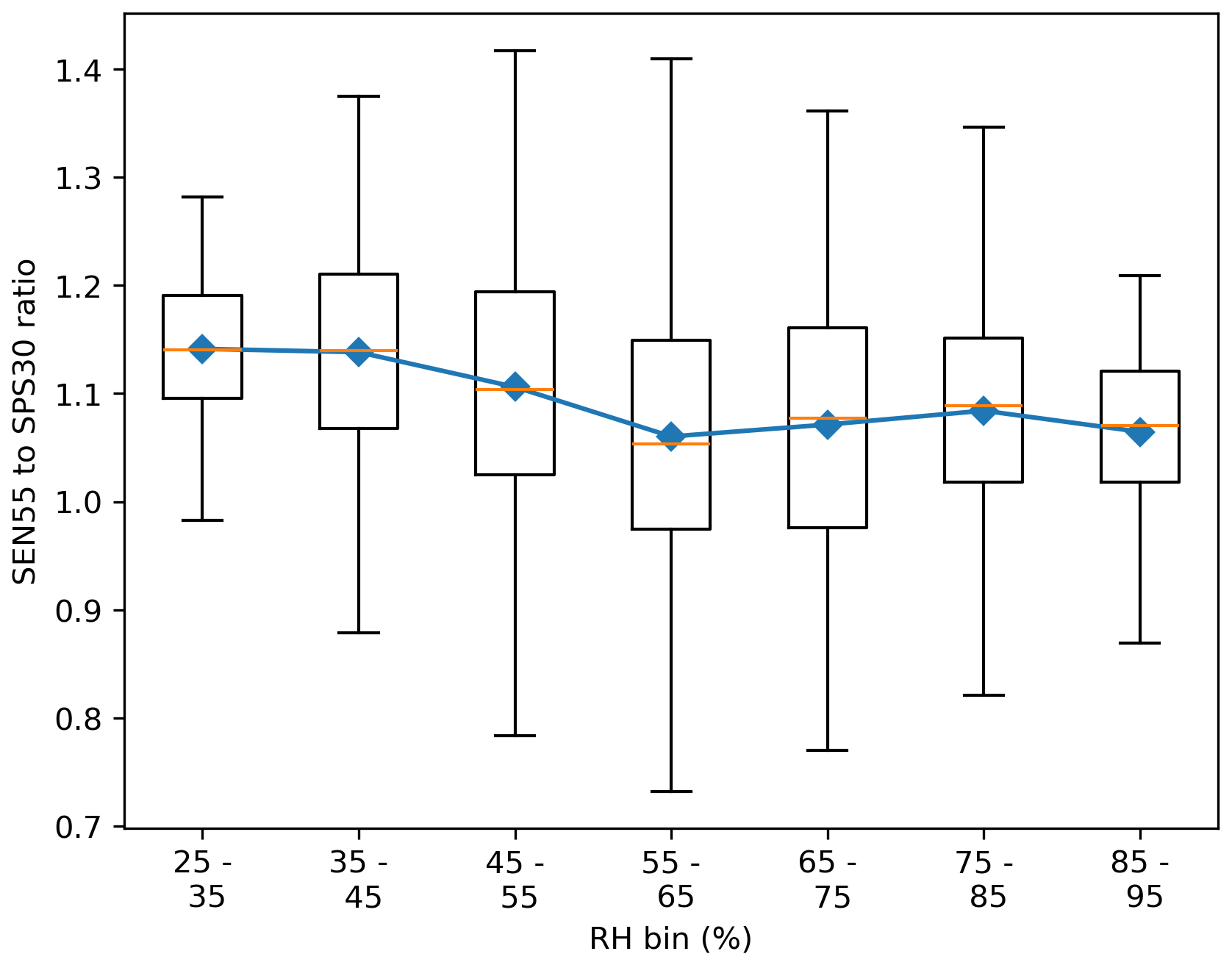
Figure H4 SEN55 to SPS30 ratios of ten-minute averages at Hyltemossa. The boxes show 25 % to 75 % percentiles of the data (Q1 and Q3). The whiskers extent to $\mathrm{1.5}\cdot (\text{Q3}-\text{Q1})$ below Q1 and above Q3. The blue line and markers show the average per bin.

Only on the lower end of relative humidities (25 %–65 %) there is a downward trend. Although an OLS regression indicates a statistically significant negative slope ($-\mathrm{6}\times {\mathrm{10}}^{-\mathrm{4}}$ per % RH, p<0.001), the magnitude of the effect is small, corresponding to a change of ∼4 % across the full RH range. There is no evidence for a meaningful effect of RH on the SEN55 to SPS30 ratio, and we can therefore assume that any effect from RH for the SEN55 is similar for the SPS30.

H4 The effect of relative humidity on sensor to Palas Fidas ratio

Since any effect of RH is similar for the SEN55 and SPS30 (see Sect. H.3), we only evaluate the effect of RH for the SEN55 versus the Palas Fidas measurements. With Eq. (5) we can calculate expected growth factors based on relative humidity GF(RH), with a κ-value of 0.3 (as measured in rural South-Sweden) (Fors et al., 2011). If the SEN55 measurement data is affected by hygroscopic growth as predicted by the κ-Köhler theory, we should see an increase relative to gravimetric measurements with increasing relative humidity, and no such increase when dividing the data points by their respective growth factors. Figure H5 shows the absolute and relative SEN55 to Palas Fidas differences (with averages per 10 % relative humidity bin), for both uncorrected and GF-corrected data. We present GF-corrected data both with corrections based on SEN55 RH, and based on PF RH.

Figure H5 Differences between SEN55 and Palas Fidas (PF) hourly averages: absolute (SEN55−PF) and relative ($(\text{SEN55}-\text{PF})/\text{PF}$), for uncorrected values (a, b), GF-corrected values (c, d), and GF-corrected values based on PF RH (e, f).

Starting from the 50 %–60 % relative humidity bin, there is an upward trend towards higher relative humidities (Fig. H5a and b). The trend across the whole range of relative humidities is significant (0.05 µg m⁻³ change in absolute difference per % RH and 0.01 change in relative difference per % RH, p≪0.001), implying an estimated 3 µg m⁻³ change over the 30 %–90 % humidity range. When corrected with κ-Köhler, there is a slight significant downward trend in the absolute difference (Fig. H5c, −0.01 µg m⁻³ change in absolute difference per % RH). In other words, the SEN55 concentrations are affected by relative humidity, at a level close to what is calculated with the κ-Köhler theory. The correction is conducted with the SEN55 measured relative humidity. When using the relative humidity as reported by the Palas Fidas, the calculated growth factors are significantly higher, resulting in an extreme underestimation (Fig. H5e and f).