A tuneable framework for outlier detection in PM_2.5 air sensor networks during wildland fire smoke events

In recent years the use of air sensors has rapidly expanded across North America to measure fine particulate matter (PM_2.5), particularly in response to increasing air quality impacts from wildland fire. With the benefit of enhanced spatial and temporal coverage, the scientific community and the public have come to rely on sensor networks as valuable sources of air quality information. With an increasing variety of sensor devices being deployed, there is a need to validate and harmonize PM_2.5 data between different device types. While significant attention has been given to calibration and correction equations to improve the accuracy of a given sensor's measurement, there is a need to develop tractable and generalizable methods of identifying malfunctioning or unreliable sensors, given the maintenance, siting, and operation of many of these devices is unknown. In this paper, we propose a method of identifying outlier PM_2.5 sensors, defined as those whose measurements deviate strongly from other local measurements due to hardware faults or to hyper-local environmental conditions that are not representative of typical ambient air quality conditions. While detecting outliers during typical conditions is a fairly straightforward task, detecting outliers during smoke events is challenging due to real, erratic shifts in PM_2.5 concentrations. Here, we present a novel method of detecting outliers within sensor networks by combining measures from information theory and machine learning. We first define a tuneable, rule-based detection function that balances the Shannon entropy of a local network against the information content of an individual sensor's measurement. We then use this function, together with additional information-theoretic and short-term temporal features, to train a gradient-boosted decision tree for automated outlier detection. Hourly PM_2.5 measurements from various device types were collected for 11 smoke events across North America in 2024 and 2025, and a stratified sample of sensor data were perturbed to simulate 5 commonly seen faults. In each of these cases, we assessed each method's ability to detect the simulated faults. We demonstrate that either of these methods can act as an adjustable data validation procedure when applied to both real-time air quality reporting and retrospective analysis for smoke impacts.

1 Introduction

Smoke from wildland fire affects millions in North America each year, contributing to thousands of deaths and a multitude of adverse health outcomes (Reid et al., 2016; Gould et al., 2024). The fine particulate matter (PM_2.5, particles with aerodynamic diameters smaller than 2.5 µm) released from wildland fire smoke is of particular concern, as exposure is strongly associated with a number of negative health effects (Schwartz et al., 1996; Pope et al., 2002; Brook et al., 2010). Populations in North America are being exposed to substantially higher levels of smoke-related PM_2.5 now than they were two decades ago, with wildfire smoke contributing up to one-quarter of annual-average PM_2.5 exposure across the United States (Burke et al., 2021; Burke et al., 2023). Recent projections indicate that increases in wildfire smoke could result in tens of thousands of additional deaths annually in the United States by mid-century, with associated economic damages on the order of USD 600 billion annually (Qiu et al., 2025). Evaluating these health impacts requires estimation of population-level exposure to PM_2.5 at a fine spatiotemporal resolution using ground-based air quality observations.

While many parts of North America, particularly large population centres, are covered by regulatory PM_2.5 monitoring networks, these stations are sparse in smoke-prone regions (Kelp et al., 2022). This limits the ability to accurately assess exposure levels in the communities most frequently affected (Larkin, 2019). Additionally, these observational gaps make it difficult to resolve the full extent and progression of smoke events in space and time, as smoke events are episodic and highly variable in duration, magnitude, and spatial extent. With increasing frequency of smoke events, a large number of publicly owned, “low-cost”, outdoor PM_2.5 sensors have been deployed across North America in recent years, with over 18 000 on the AirNow Fire and Smoke Map in 2025 (https://fire.airnow.gov, last access: 7 April 2025). Sensor networks have shown promise in increasing the resolution and accuracy of population-level exposure models, furthering understanding of the distribution of air quality impacts (Clements et al., 2017; Morawska et al., 2018; Bi et al., 2020; deSouza et al., 2020; Keyes et al., 2023; Raysoni et al., 2023).

While expanded monitoring across the United States has furthered our ability to assess wildfire smoke exposure, sensors come with their own set of challenges. Sensors are being developed by a variety of manufacturers, each with unique hardware designs, firmware configurations, and proprietary calibration strategies, making data harmonization across networks a growing challenge. While substantial attention has been given to increasing the accuracy of sensor measurements through calibration and correction equations to account for source pollutant characteristics and environmental factors (Zimmerman et al., 2018; Malings et al., 2020; Barkjohn et al., 2021; Raheja et al., 2023), significant challenges remain. Sensors vary in build quality, stability, and the operation and maintenance practices they receive, and may fail unexpectedly through hardware defects or insufficient protection from environmental elements. Common faults include power loss, communication failure, data corruption, hardware malfunction, and firmware error (Barkjohn et al., 2025a). When aggregating air quality data, faulty sensors often manifest as statistical outliers within a network, either as persistently low or high extreme values, flatlined readings, abrupt baseline shifts, or unusual divergence from collocated measurements. Even if the device is performing as intended, privately operated sensors may produce aberrant measurements. They may be sited incorrectly, exposed to an emission source at close range, or deployed deliberately to capture conditions of interest: a homeowner may site a sensor at their own property, while a clean-air agency may place sensors to capture prescribed smoke or other emissions in an area of concern. We define these as hyper-local conditions that influence a single sensor, such as a barbecue, a house fire, woodstove emissions, an outdoor sensor being moved indoors during a smoke event, or other personal-use scenarios. These can alter public health messaging that is reliant on community measurements and confound network-scale analyses. As sensor networks continue to expand, enabling broader spatiotemporal coverage, it will be increasingly important for users of sensor data to implement automated fault detection and normalization strategies that can identify these outliers without sacrificing data integrity.

Automatic fault detection is especially challenging due to the unequal spatial distribution of sensors (deSouza and Kinney, 2021) and the highly variable scale and magnitude of smoke events, which can produce gradients of PM_2.5 concentrations that may be sharp, patchy, and transient over small distances (Jaffe et al., 2020), and further exacerbated by terrain, where topographic features can channel, pool, and disperse smoke in ways that decouple nearby sensors (Kochanski et al., 2019). To overcome these challenges, a useful definition of representativeness must be agnostic of sensor manufacturer, scale with varying network densities, and account for the timing and variability of PM_2.5 concentration shifts across networks. Additionally, methods must account for the fact that many sensors are intentionally deployed in pollutant hotspots (Madhwal et al., 2024; Sablan et al., 2024) where elevated concentrations or abrupt spatial variability may be real and meaningful rather than indicative of faulty measurements (Barkjohn et al., 2025a). Thus, a robust outlier detection framework will need to maintain tolerance for disagreement within the network during smoke intrusion into a region, while maintaining sensitivity to correctly identify true faults.

Recent work has explored graph-based methods that utilize the collective behaviour of sensor networks to validate sensor measurements. These include graph signal processing (Ferrer-Cid et al., 2022) and graph neural networks (GNNs). GNNs learn the relationships between nodes (here, sensors) to predict each node's reading and flag departures from those predictions (Deng and Hooi, 2021). They have been applied to a large low-cost PM_2.5 network (Wu et al., 2023), and Ferrer-Cid et al. (2025) review graph-based approaches to sensor data quality. However, such approaches depend on either gradual measurement variation or a historical relationship between network members, both of which may break down during wildfire smoke events. GNNs and other machine learning methods are reliant on extensive training data, which is scarce for sensor faults. Models may be biased towards learned historical relationships between sensors, which suit spatially continuous fields and stable sensor biases, such as temperature, but not episodic phenomena like smoke. The difficulty is illustrated by Zafeirelli et al. (2026), who applied temporal and spatial outlier methods to PurpleAir data during the August 2021 Athens wildfires and found that separating sensor errors from genuine smoke-driven signals required combining methods with distinct sensitivities to localized and widespread events.

In this work, we build on this general idea of network-informed detection but adapt it to the complexity of smoke events by designing a generalizable approach that infers a device's validity from a local network of nearby devices (which may include both regulatory-grade PM_2.5 monitors and sensors), tolerates local network disagreement, incorporates temporal variability, and remains robust to the shifting structure of inter-sensor relationships during smoke events. By using a dataset of PM_2.5 observations during 11 smoke events across North America in 2024 and 2025, we simulate common fault types in existing sensor networks and optimize an algorithm to identify them. Using measures of entropy and information from the field of information theory, we define and optimize a rule-based equation that is tuned for identifying outliers at an hourly resolution. We then expand upon this concept and train a gradient-boosted decision tree model using our outlier detection function in the feature set. The results from these models, and their practical implications when applied to continental-scale sensor networks, are discussed.

2 Data Sources and Study Design

2.1 Study Design Overview

This study proceeds in two phases. The first focuses on method development, parameter tuning, and benchmarking using a selection of curated smoke events (Sect. 2.3) and sensor networks, where we create a semi-synthetic dataset with introduced sensor faults. This phase includes an evaluation against conventional neighbour-comparison methods (Sects. 3 and 4). The second applies a subset of these methods to 9 months of continental-scale data and validates the detections by hand (Sect. 5).

For phase one, we collected ground-based PM_2.5 observations during 11 wildfire smoke events that occurred in North America in 2024 and 2025. Data were collected from several types of PM_2.5 measurement devices including regulatory permanent monitors, temporarily deployed reference-grade monitors, state-developed sensors, and publicly deployed sensors that were active during the smoke events. Air quality devices were grouped into networks at several spatial distance thresholds, creating lookup tables between any given device and its neighbouring devices. For each smoke event, a random, stratified sample of devices was selected to have its data perturbed to simulate a fault. This included both monitors and sensors, and for the purpose of our analysis, these devices were treated the same. Five types of faults were introduced to each device, perturbing the data of only one unit at a time during a given event. In total, 176 devices were used to simulate potential outliers, resulting in 880 different scenarios to evaluate the ability of our methods to detect perturbations.

In phase two, we test whether the methods and parameterizations developed in phase one generalize beyond the curated events. We applied eight parameterizations of the outlier detection methods to 9 months of air quality data (1 January–30 September 2025), drawn from the same device types and data sources as phase one, extended to all reporting devices across the United States (including Alaska and Hawaii) and Canada: 19 562 unique PM_2.5 devices reporting at least once during the period. This window spans both network-scale baseline conditions and smoke events of varying magnitudes and network structures, allowing us to evaluate whether tuning on semi-synthetic perturbations transfers to real-world variability. We manually evaluated flagged detections to determine whether they represented faulty devices, hyper-local events, or misclassifications (i.e., well-performing sensors).

2.2 Air Quality Data

Air quality data were collected for four different categories of devices: Permanent monitors, temporary monitors, state-developed sensors, and publicly owned sensors. These data came from AirNow, the Western Regional Climate Center temporary monitor archive, and the PurpleAir API. State-developed sensors included SensWA and SensOR networks. The temporary monitors have shown reasonable agreement with the Federal Reference Method network (Schweizer et al., 2016), state-developed sensors are operated and corrected according to state data-quality practices (Washington State Department of Ecology, 2024a, b; State of Oregon Department of Environmental Quality, 2023, 2026; Molina Rueda et al., 2023; Johnson, 2024), and PurpleAir data were screened for agreement between their duplicate measurement channels (Barkjohn et al., 2022). Sensor measurements were corrected using device-appropriate correction equations, including the extended United States-wide PurpleAir correction (Barkjohn et al., 2025b), to improve comparability with monitor measurements. Device-specific hardware, correction procedures, quality criteria, and processing details are provided in the Supplement and Table S1.

2.3 Smoke Event Selection

We define a smoke event as a geographic region impacted by elevated PM_2.5 concentrations from wildland fire. The sites used in this study were selected from known events in 2024–2025 with sufficient PM_2.5 monitor and sensor coverage that the extent of impacted devices in the region was evident in the observational data. There were 10 geographic sites used, and 11 total events (Fig. 1, Table 1), with one geographic area used for both an event caused by regional wildfire (WF) smoke, and another event due to a local prescribed fire (Rx).

Figure 1 Map showing the location and geographic extent of the 10 geographic sites used, and PM_2.5 monitors and sensors with recorded observations during the study period. (Basemap sources: Esri, USGS, NGA, NASA, CGIAR, NOAA | Powered by Esri.)

The events were identified by manual judgement rather than by a programmatic detection scheme. Candidate events were drawn from either known events, or by reanalysing air quality impacts over the study period and were contextualized using satellite fire detections and smoke plume extents from NOAA's Hazard Mapping System (HMS; Rolph et al., 2009; Brey et al., 2018) and known fire incidents from the National Interagency Fire Center (NIFC, https://www.nifc.gov/, last access: 14 September 2026). Events were attributed to prescribed fire when they occurred outside the climatological fire season (NWCG, 2026) and coincided with small, short-lived satellite fire detections nearby. Event windows were then delineated by inspection of network PM_2.5 time series, bounded by the return to lower ambient concentrations. We deliberately did not derive events from a satellite-based smoke product, given that such products can indicate smoke aloft as well as surface impacts, and translating them into surface smoke days requires regionally calibrated filtering (Liu et al., 2024), a research problem outside the scope of this study. For our purpose of smoke-impacted periods in which to detect outliers, hand curated events are sufficient, and per-event characterization (satellite fire detections, satellite-derived smoke plume coverage by day, and network AQI time series) is provided in the companion materials (Illson, 2026b).

These site extents are analyst-defined bounding regions used to subset devices for analysis and do not necessarily delineate the full extent of smoke.

Table 1 Site names, smoke source (wildfire, WF or prescribed, Rx), spatial extent, and the date ranges used in capturing the smoke event. Includes the number of monitors (Permanent or Temporary) and the number of sensors (PurpleAir, SensOR, or SensWA), and the number of devices (includes both monitors and sensors) perturbed to simulate outliers.

Consideration was given to selecting a diverse range of sites and smoke events. Rather than focusing solely on regions with the most frequent smoke events, sites were chosen to represent a range of conditions, including urban and rural settings, impacts from both WF and Rx smoke, localized vs. regional smoke events, topographically complex vs. flat regions, dense vs. sparse networks of sensors, and differing environmental regions (additional details Illson, 2026b).

3 Methods

3.1 Network Generation

To construct local networks of monitors and sensors, one-to-many lookup tables were generated at multiple proximity thresholds, grouping any given PM_2.5 monitor or sensor to others based at that proximity. First, each measurement location was assigned a unique identifier based on a combination of the devices' given ID and latitude/longitude coordinate pair. This was necessary because many sensors and temporary monitors relocate or may report coordinate differences over time. Device coordinates were reprojected into the North America Albers Equal Area Conic projection (ESRI:102 008) to enable distance calculations in meters. Neighbouring units were then identified using a pairwise two-dimensional Euclidean distance threshold, implemented with the libpysal Python package (Rey and Anselin, 2007).

Networks were generated at eight spatial thresholds, ranging from 2.5–20 km in 2.5 km increments. We further reduced the number of network proximities for evaluation by considering the spatial distribution of devices and the need to balance proximity with a sufficient number of neighbouring devices. Considering the first law of geography that “everything is related to everything else, but near things are more related than distant things” (Tobler, 1970), smaller thresholds may produce networks that capture shared conditions, however, identifying faulty behaviour within a network also requires a minimum number of devices to establish consensus. This balance was complicated by the uneven distribution of sensors across North America (deSouza and Kinney, 2021). The PurpleAir sensors are disproportionately concentrated in California, especially so in the 9 counties that comprise the Bay area – Alameda, Contra Costa, Marin, Napa, San Mateo, Santa Clara, San Francisco, Solano, and Sonoma. At the time of analysis in early 2025, we found 18 % of all PM_2.5 monitors and sensors in North America were located within these 9 counties, with the overwhelming majority being PurpleAir sensors. At 21 220 km², these counties cover only 0.23 % of the total United States land area, yet disproportionately skew our results for how many neighbouring devices a sensor or monitor will have at a given proximity (Fig. S1 in the Supplement). To strike a balance between spatial proximity and sufficient network density, we focused on thresholds where at least half of the devices located outside the Bay Area counties had three or more neighbours. This ensured more consistent network structure across the broader sensor distribution. For our analysis, we elected to use networks 5 km and larger, ensuring that at least half of devices had at least three neighbours.

Network connectivity evolves over various spatial thresholds, and in complex terrain, this can link devices in different drainage basins. An example can be seen in Fig. 2, at the Methow Valley, WA site. This has the potential to introduce network disagreement, when wildland fire smoke becomes trapped in valleys due to radiative feedbacks that reinforce local stability and suppress mixing (Kochanski et al., 2019). In very dense networks, such as Los Angeles, CA, these one-to-many networks can become incredibly large and redundant, with devices having greater than 200 connections even at modest thresholds. To maintain tractability and reduce computational requirements, we limited the tuning networks to a maximum of 20 neighbouring devices, keeping only those closest to our device of interest.

Figure 2 Example of PM_2.5 sensor networks in the Methow Valley, WA, generated using two spatial thresholds: 7.5 and 20 km. Each point represents a PM_2.5 monitor or sensor, and lines indicate connections based on the selected proximity threshold. As the distance increases, overall network connectivity increases, linking devices across drainages. Line colour corresponds to device latitude, to help trace where connections originate. (Basemap: © MapTiler; © OpenStreetMap Distributed under the Open Data Commons Open Database License (ODbL) v1.0; for further information, please see https://www.openstreetmap.org/copyright/en, last access: 14 September 2026.)

3.2 Simulated Fault Generation

A semi-synthetic dataset was constructed by injecting simulated faults into the real-world PM_2.5 time series data from each of the smoke events. For each event, we collected eligible devices (both monitors and sensors) that had at least three neighbours within 5 km. A random subset of these eligible devices was sampled. We sampled 40 % of eligible devices if fewer than 25 devices were present within the site footprint, 10 % if more than 100 were available, and 20 % otherwise. For the purpose of our analysis, these devices were treated the same because the method is intended to detect departures from local network agreement rather than instrument-specific failure modes. This choice also broadens the method's applicability across device classes, including temporary monitors and future PM_2.5 devices with different noise characteristics, sampling intervals, or correction workflows.

For each selected unit, five unique fault types with different perturbations were applied, introducing only one into a network within a smoke event at a time. The perturbations occurred for a continuous interval, randomly ranging from 8–48 h in duration, keeping within a 3 h buffer from the beginning or end of the time series. Fault types were designed to emulate realistic sensor anomalies:

1. Fixed high (Fault type 1). The device becomes fixed at a high value, intermittently dropping out due to either failing QA/QC or electronic malfunction.

2. Off then low (Fault type 2). The device goes offline, then returns reporting a lower value – such as when an outdoor sensor is moved indoors.

3. Stuck value (Fault type 3). The device becomes stuck and reports a single value without responding to ambient conditions.

4. Amplification (Fault type 4). The device measurement is amplified by a random factor increasing it by 75 %–100 % of the original value.

5. Noise (Fault type 5). Erratic and high-frequency noise is applied to the value.

Figure 3 illustrates examples of each of these perturbations applied to a device. The code to generate similar synthetic faults is provided in the supplemental material.

Figure 3 Time series showing how a randomized, synthetic fault is applied to a PM_2.5 device. Time series of hourly averaged PM_2.5 measurements converted into EPA AQI for a single sensor (solid black line) and devices within its network (dashed grey lines) during a smoke event. The top-left panel shows the unperturbed time series for reference. The remaining panels display the impact of each fault type, highlighted by the shaded period. Background is coloured by EPA AQI category ranges.

3.3 Information-Theoretic Outlier Detection

3.3.1 Applicability of Information Theory

For this work, we investigated whether the fundamental measures of information theory could validate a PM_2.5 sensor's measurements within the context of its local network. The two principal concepts, entropy and information content, offer potential utility in interpreting sensor and network behaviour.

In the context of a PM_2.5 sensor network, entropy measures the variability of measurements within the network: the degree of disorder, or unpredictability, in what nearby devices report. High entropy reflects disorder or instability, such as conditions where smoke intrusion is causing nearby devices to report drastically different measurements. Conversely, low entropy indicates a broad agreement and stability across the network. The information content of a device within its network reflects the unexpectedness, or surprise, of a given value being seen relative to its network. This allows us to not only characterize the state of the network as a whole, but to identify individual devices that deviate from their local network. These information-theoretic concepts work together, allowing us to accommodate networks of varying size and device type, while providing measures of disorder whose interpretation remains consistent across network scales, even during smoke events.

It is important to note that Shannon entropy and Shannon information (Shannon, 1948) were formulated for discrete variables. In both public health and regulatory contexts, PM_2.5 values are typically converted into discrete air quality categories, such as the EPA's Air Quality Index (AQI) (https://www.airnow.gov/aqi/, last access: 14 September 2026) or the Canadian Air Quality Health Index (AQHI) (Stieb et al., 2008). These categorical bins are tractable, widely understood, and grounded in communicable risk levels, making them a natural starting point in determining whether two sensors are in agreement. This categorization avoids overemphasis on minor numerical differences and simplifies the categorical comparison that our detection rule optimizes. We consider it sufficient for broad outlier detection, with the practical benefit that flagged disagreements correspond to the categories immediately visible on public health resources such as AirNow and the Fire and Smoke Map.

Information theoretic methods inherently scale with network density, adapting to situations with many or few neighbouring observations without the need for reparameterization. Moreover, because these measures quantify uncertainty itself, they remain meaningful in disordered and rapidly evolving networks, making them robust to the complex, shifting patterns that occur during smoke events. Entropy has been used in guiding the design and evaluation of environmental monitoring networks in hydrometry (Keum et al., 2017), and mutual information underpins classical algorithms for sensor placement (Krause et al., 2008); in PM_2.5 networks specifically, value of information has recently been applied to design placement strategies under multimodal data fusion (Choi and Hummel, 2026). Here we apply these measures to a different task: characterizing the instantaneous state of a PM_2.5 network. One of the key advantages of applying information theory in this context is that it enables the detection framework to defer classification during periods of high uncertainty when the network becomes disordered, avoiding premature characterizations during rapidly evolving smoke events. Because the approach is contingent on network agreement, its sensitivity can be tuned to tolerate varying levels of disorder across spatial proximities or event types, from highly localized anomalies to region-wide smoke intrusions. This prevents the removal of potentially valuable data under unstable conditions, while allowing temporal averaging and threshold adjustments to modulate the aggressiveness of outlier detection as desired.

3.3.2 Rule-based Detection Equation

We define a rule-based outlier detection equation that uses a set of adjustable thresholds to flag measurements that match specified criteria. The equation relies on conditional logic to assess a given device's measurement relative to its local network. This equation is applied to a single device at a time, and utilizes the current measurement of the device and the current measurements within its network. All measurements are assigned to categorical bins rather than compared as numeric concentrations and we used the AQI and a custom bin set that modified the AQI thresholds to soften the transitions. This binning aligns flagged disagreements with the air quality categories that public health officials and the public act on (AirNow, 2026).

First, we compute the network entropy H_k for device k, which reflects the degree of disorder in the distribution of observed categorical AQI bin values x∈X, reported by the device and its local network:

$$\begin{array}{}\text{(1)}& H_k=-\sum _{x\in X}p\left(x\right){\log }_{\mathrm{2}}\left(p\right(x\left)\right)\end{array}$$

where p(x) is the proportion of neighbouring devices whose measurements fall into AQI bin x. A lower entropy value indicates that neighbours are clustered in a small number of categorical bins (more ordered, less uncertain). Conversely, a higher entropy value indicates a broader distribution of observed bins.

Second, we compute the information content I_k of the device's bin category with respect to its network, representing how uncommon that value is relative to observed bins in the network:

$$\begin{array}{}\text{(2)}& I_k=-{\log }_{\mathrm{2}}\left(p_k\right)\end{array}$$

Higher values of information content indicate observations that deviate more strongly from expectation, carrying greater “surprise” in the information-theoretic sense. Such measurements are less probable within the local distribution. In this context, they correspond to more surprising or infrequent bin classifications relative to those of neighbouring devices.

Third, we calculate the bin deviation D_k, defined as the absolute difference between a device's bin index and the mean bin index of all other devices in the same local network at the same time step. For a network of N devices, where B_k denotes the bin index assigned to device k:

$$\begin{array}{}\text{(3)}& D_k=\left|B_k-{\displaystyle \frac{\mathrm{1}}{N-\mathrm{1}}}\sum _{\begin{array}{c}j=\mathrm{1}\\ j\ne k\end{array}}^N{B}_j\right|\end{array}$$

Here, the summation is taken over all devices in the network except device k, and the summation represents the mean bin index of the remaining N−1 devices. Note that B_k refers to the bin index (an integer from 1 to the number of bins), distinct from the bin boundaries x used to define concentration intervals in Eq. (1). Because information content is based on the probability of discrete bin values, it reflects how rare a value is within the network but not how far that value is from the norm. For example, an observation in a rarely occupied bin will yield the same information content whether it is close or far in measurement space. A network with 49 observations in the lowest AQI bin and 1 in the highest produces the same entropy as one with 49 in the lowest and 1 in the second-lowest bin. D_k captures this distinction, quantifying how far in measurement space an observation of B_k may be from the network average.

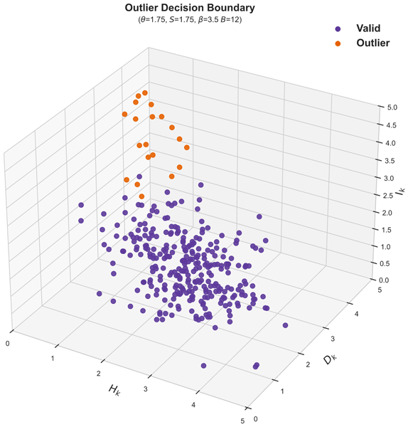
Finally, the detection rule is implemented using a conditional logic statement, which flags a unit as an outlier only if all three conditions are met:

$$\begin{array}{}\text{(4)}& {\mathrm{\text{Outlier}}}_k=\left\{\begin{array}{ll}\text{True},& \text{if}{I}_k^{\left(r\right)}\ge \mathit{\theta }\text{and}{H}_k^{\left(r\right)}\le S\text{and}{D}_k^{\left(r\right)}\ge \left(\frac{B}{\mathit{\beta }}\right)\\ \text{False},& \text{otherwise}\end{array}\right.\end{array}$$

I_k – Information value of device k, H_k – Network entropy value for device k's network, D_k – Absolute difference between device's bin and the mean network bin, r – spatial proximity threshold for defining the network around device k, θ – Information coefficient, S – Network entropy coefficient, β – Bin coefficient, B – Number of possible bin values.

This equation flags outliers by evaluating a device's measurement against its local network at a given spatial proximity r. We can adjust several inputs and thresholds, with the overall goal being to select instances where a device's measurement (i) exists in an ordered network (low entropy); (ii) has a high information content relative to the network; and (iii) is sufficiently distant from the average bin category of the network (see Fig. 4). We adjust the bin coefficient β by the number of possible bin values B. This is an attempt to help the equation remain transferrable across different binning schemes or air quality index classification systems.

Figure 4 Three-dimensional visualization of the decision boundary created by the outlier detection equation. The decision rule optimizes for outlier detection given the device measurements in the context of the device's network. We tune the equation for measurements that (i) exist in an ordered network (low entropy); (ii) have a high information content relative to their network; and (iii) are sufficiently distant from the average bin category of the network.

3.4 Parameter Tuning

The goal of tuning our equation is to maximize the number of hours in this time series where we correctly identify the perturbed measurements (recall), while not misclassifying any valid measurements (precision). For our rule-based equation, there are a total of 5 configurable inputs, which may be tuned to optimize its performance. These are: (1) the local network at proximity r; (2) the number of bins B and what concentration ranges they represent; (3) how much network entropy to allow S; (4) how much information is required θ; and (5) how many bin steps are sufficiently far away in measurement space D_k.

We selected both the F₁ score and F_β score (β=0.5) as objective functions to tune our thresholds with, reflecting two tuning priorities: balanced performance (F₁) and precision-weighted performance (F_β=0.5). In a classification context, the F₁ score gives equal weight to precision and recall, F_β=0.5 increases the weight on precision relative to recall meaning that F_β=0.5 will generally lead to fewer false positives and also fewer real outliers being flagged than F₁. Compared with accuracy, F₁ and F_β scores are more appropriate for imbalanced datasets such as ours where outliers are relatively rare. Metrics such as area under the receiver operating characteristic curve (AUC-ROC) and precision-recall curves are less directly applicable in this context, as our decision rule outputs discrete class labels rather than continuous scores. The F₁ and F_β scores provide interpretable summaries of this trade-off of the classifier performance at a given parameter set.

To ensure meaningful optimization and keep computational runtime within reason, we constrained the parameter search space. For example, entropy thresholds had to allow some variability while excluding cases of complete disorder, and bin deviation thresholds needed to distinguish measurements that were meaningfully different in measurement space. Without such constraints, it is possible to arrive at configurations that minimize false positives by trivially classifying nearly all data as valid.

We conducted a grid search applying 8400 unique parameter combinations to 880 time series containing a synthetic fault, totalling over 7.2 million evaluation runs. The parameter sweep utilized spatial proximity thresholds ranging from 5000–20 000 m in 2500 m increments, S and θ limits from 1.4–2.3 (in 0.1 increments), β from 1.5–4.0 (0.5 increments), and two binning strategies: EPA AQI and a modified EPA AQI (hereafter the “modified AQI”; denoted “pct” in method identifiers after the percentage-based overlap of its transition bins) where bins were added to overlap the breakpoints between categories (Fig. S2). These breakpoints covered the lower 10 % of the next highest category and the upper 10 % of the next lower category, which result in a doubling of categorical bins, totalling 12 bins. This modified EPA AQI was done to test softening the transitions of the AQI categories, since for example a sensor could be only 1 µg m⁻³ higher than its neighbours and be in a different AQI category. This search enabled us to identify parameter configurations that achieved optimal trade-offs between detection sensitivity and false positive rates across fault types and network configurations.

The grid search was conducted entirely on the 880-series semi-synthetic benchmark; no synthetic data were held out for testing, and independent evaluation of the tuned configurations comes from the continental-scale application (Sect. 5). Within the search, each configuration was scored against the measurable-outlier criterion evaluated at that configuration's own bin coefficient β. This reflects a scoping choice, since the bin coefficient jointly sets the detection threshold and what is defined as a measurable outlier. Note that this criterion compares the perturbed measurement with the device's own unperturbed value, measured in categorical bins; it is distinct from the bin deviation (Eq. 3), which compares a device with its neighbours.

3.5 Gradient-Boosted Decision Tree

While the rule-based detection equation provides a straightforward and interpretable method for identifying outliers, two limitations follow directly from its construction. First, it can only flag deviations large enough to register categorically, a fault that does not shift the measurement far enough categorically is invisible by design. Second, it evaluates each hour as an independent snapshot, with no temporal context from the device or its network. To address both, we extend the detection framework with the antecedent behaviour of the device and its local network, seeking signals that a device is diverging from its neighbours before, or without, a categorical deviation ever appearing. This temporal context is aimed particularly at faults that may go undetected. How, for example, can a faulty device be identified when both its measurements and its network are very low, or very high?

Machine learning is particularly well suited to this task, offering the ability to model complex, nonlinear relationships from multivariate time series data. Gradient-boosted decision trees (GBDTs), in particular have stood out as a powerful and commonly used class of model that excels in classification problems (Friedman, 2001; Chen et al., 2018; Bentéjac et al., 2021). We chose to use the popular eXtreme Gradient Boosting (XGBoost) software package (Chen and Guestrin, 2016), due to its ease of use and robust history of application to a wide range of problems in the environmental sciences and beyond. XGBoost fits the structure of this problem since our features are tabular and heterogeneous, a setting in which gradient-boosted trees consistently perform as well as or better than more complex model classes, without feature scaling or architecture design (Grinsztajn et al., 2022; Shwartz-Ziv and Armon, 2022). The algorithm natively handles the missing values that are routine in sensor networks and the severe class imbalance of our training data; trained models are computationally light enough for hourly scoring across tens of thousands of devices; and feature-importance measures keep the model's decisions partially interpretable.

3.5.1 Model Features

Several model features were generated to characterize the recent-to-current behaviour of the measurement signal, with the idea that naturally fluctuating PM_2.5 measurements during a smoke event might behave differently than those being recorded by a faulty sensor. These include features on a per-device basis which measure the relative variability of PM_2.5 measurements, the trending directionality of measurements over a time window, recent outages, the range of recent measurements within a time window, the entropy of recent measurements within a time window, and how these values contrast with the behaviour of the local network. Also included were the information theoretic measures of device entropy and information within its local network, a true/false flag for whether our rule-based equation detected an outlier, and some network density data quantifying how many devices existed within various proximities. The full set of features, along with the time windows used in their generation, are listed in Table S2.

For our information theoretic features (measurement entropy, network entropy, device information, and outlier detection flag), we had to constrain our runs to use the parameter inputs discussed in Sect. 3.3. We trained the model using a total of 8 parameter sets, varying several factors. We used a central cluster of proximities (7500–12 500 m), two binning strategies (the EPA AQI and the modified AQI; Sect. 3.4), and two settings of the entropy and information thresholds drawn from the tuned configurations.

3.5.2 Model Training

We trained several binary classification models using XGBoost to detect our synthetic faults, trying to identify measurements that had been perturbed by one of our fault methods. Each model was trained using differing combinations of features, parameterizations passed through from the rule-based equation methods used, and alternative PM_2.5 binning strategies. All variations underwent identical training protocols. Performance of the top models will be described in the next section.

Labels for the supervised classification come from the fault-injection process: every device-hour within a perturbation window is a positive example, every other device-hour a negative one. This training target, an induced fault hour, is intentionally broader than the measurable-outlier criterion used to evaluate the rule-based equation, because the model is asked to identify every hour of an induced fault, not only the hours in which the fault produces a measurable change. By design, the perturbed measurements (fault occurrence) in our training data were rare compared to true observations, and the dataset exhibited significant class imbalance, with only ∼1 % of the observations labelled as perturbations, corresponding to a positive-to-negative ratio of approximately 1:90. To address this, the model was configured to apply increased weight to the minority class during training, directly proportional to this imbalance.

These models were trained and evaluated using five-fold cross-validation. In each fold, the data was split into training and validation subsets, allowing the model to be assessed on unseen data. For each fold, approximately 80 % of the data were used for training and 20 % for validation. We used a maximum tree depth of seven and applied conservative regularization, including subsampling of both rows and features, to reduce the risk of overfitting and encourage generalization. The models were trained using the binary logistic loss function and its performance was evaluated using multiple metrics, including the F₁ score, F_β=0.5, (AUC-ROC), overall classification accuracy, and the log loss of the predicted probabilities.As with the rule-based equation, models were trained and cross-validated exclusively on the 880-series benchmark; out-of-sample performance is assessed on the continental-scale data (Sect. 5).

Given the class imbalance, we dynamically optimized the decision threshold for classification in each fold. This threshold was selected based on a precision-recall curve to maximize the F₁ score. To select the most representative and effective model during training, we retained the one that achieved the highest F₁ score across all folds. This approach, combined with regularization and threshold tuning, helped ensure that the final model maintained the best sensitivity to perturbations while limiting false positives.

After assessing model performance across parameter thresholds, binning strategies, and feature sets, configurations that consistently yielded the highest F₁ scores were advanced for evaluation on real-world data. The final feature sets evaluated used the features from Table S2, along with the two best parameter sets at spatial proximities of 7500 and 12 500 m.

3.6 Baseline Comparison Methods

We benchmarked the detection equation and the XGBoost models against three conventional statistical measures to compare neighbours, each computed on the same networks and hourly measurements as our methods: the absolute neighbour deviation (Shekhar et al., 2003; Janeja et al., 2010), the neighbour z-score (Shekhar et al., 2003; Zhang et al., 2010; van Zoest et al., 2018; Chen et al., 2018; Wei et al., 2020), and the robust z-score (Rousseeuw and Croux, 1993; Leys et al., 2013). The two z-score rules (the neighbour z-score and the robust z-score) were evaluated at their conventional cutoffs of 3 (Shekhar et al., 2003) and 3.5 (Iglewicz and Hoaglin, 1993), and all three rules were additionally evaluated at the cutoff that maximized their performance on our benchmark (50 µg m⁻³, 8, and 8, respectively), so that the comparison reflects neither an untuned reference nor an unrealistically favourable configuration.

Because these methods flag outliers on different measurement scales, comparisons involving the detection equation were scored against a common, method-independent definition of a measurable outlier: a perturbed device-hour in which the modified AQI bin of the perturbed measurement differs from the bin of the underlying true measurement by at least one sixth of the total number of bins ($B/\mathrm{6}$). Unlike the tuning criterion in Sect. 3.4, which scores each configuration against its own β, this definition is fixed across these comparisons and independent of measurement scale. Comparisons involving the XGBoost models instead use their training target of any perturbed hour, since that is the quantity those models are built to predict. The bin deviation (Eq. 3) is reported only as a diagnostic rather than as a competing method, because it is computed from the same bin space as this definition and the comparison would be circular.

A broad range of outlier detection techniques could be applied to this problem, such as temporal filters on a device's own record, density- and cluster-based detectors, learned models, etc. The comparison metrics presented here are not intended to be exhaustive. We limit it to instantaneous neighbour-comparison rules, which share the constraints of our data. Temporal self-comparison methods, such as interquartile-range filtering of a device's own distribution, assume a stable per-device baseline, which was an assumption that smoke events specifically violate (see Zafeirelli et al., 2026, who examine this temporal–spatial contrast for PurpleAir sensors during the August 2021 Athens wildfires).

4 Results: Semi-Synthetic Benchmark

4.1 Rule-Based Detection Performance

We evaluate the performance of our equation with respect to two considerations: its ability to detect the perturbed device at least once during the event, and how well it classifies measurable outliers (perturbed measurements whose modified AQI bin differs from the original measurement's bin by at least the categorical threshold, $B/\mathit{\beta }$) across fault types and locations. Figure 5 highlights the need for this measurable outlier definition and shows two cases where our equation is operating as designed but not classifying all perturbed measurements. Figure 5a shows how the equation will not classify measurements during periods when the network entropy is high, and detection becomes uncertain. Similarly, Fig. 5b highlights a case where the synthetic fault never deviated from local conditions enough to qualify as an outlier, and therefore the perturbation is not a measurable outlier. All metrics are computed per evaluated device: precision, recall, and F₁ follow their standard definitions over that device's hours, and the false-positive rate is the fraction of unperturbed device-hours that were flagged.

4.1.1 Detection by Fault Type

Across all induced faults where there was at least one instance of a synthetic measurement deviating from the original measurement's category, the equation successfully identified the outlier in 95.7 % of time series events across all fault types and parameter configurations, demonstrating strong overall sensitivity to our outliers. When broken down by fault type, detection rates varied moderately (Table 2). Fault fixed high (type 1) achieved the highest success rate, with the outlier detected in 98.5 % of perturbations. Fault types off then low and stuck value (2 and 3) followed, with detection rates of 90.7 % and 90.0 %, respectively. The amplification fault (type 4) was the most challenging, with a lower success rate of 82.8 %, indicating that this class of fault may present more subtle or intermittent signatures. Fault type noise (5) matched the overall performance, with 95.7 % of cases resulting in successful detection. These results suggest the general method is broadly effective across fault types as identifying an outlier from a composite time series, though performance may vary depending on the specific characteristics of the fault and parameter configurations used. These high detection rates were achieved while maintaining a very low rate of false positive detections. Across all configurations, events and fault types, the mean false positive rate was only 1.04 % with a minimum of 0.91 % for fixed high faults (type 1), and a maximum of 1.74 % for noise faults (type 5). When selecting the optimal parameter configuration for each fault type, in every test example the method demonstrated an ability to detect that given fault at least once during the smoke event.

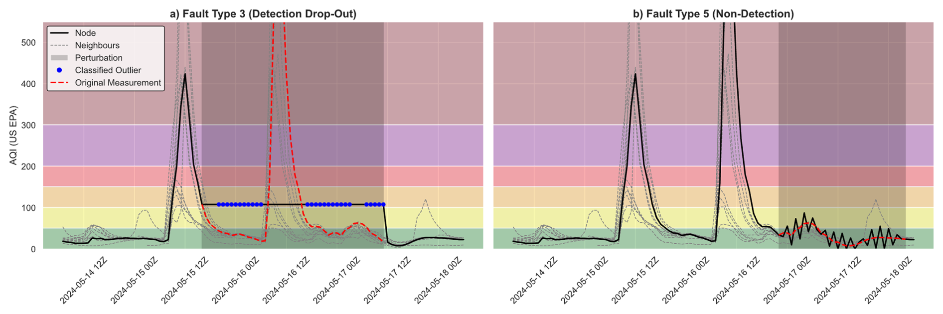
Figure 5 Time series of two different synthetic faults applied to a device, with its neighbouring network. The original device measurements shown as a black line. In panel (a), we do not classify the perturbed measurements as an outlier while either entropy is high (disorder in network), or the local network measurement average is nearby in measurement space. In panel (b), our equation skipped the noise perturbation (fault type 5) entirely due to it being contained within the same categories as the network – we do not consider this event to contain measurable outliers.

4.1.2 Parameter Configurations and Fault-Type Sensitivity

The overall classification performance of the equation varied substantially in response to fault types and parameter configurations (Fig. S3). The optimal parameter configurations exhibit both high F₁ and F_β=0.5 scores, often exceeding 0.9, which is indicative of strong recall and precision. In its optimal parameter configuration, fault type 1 was the most reliably detected, achieving an F₁ score of 0.97. Fault types 2 and 3 followed with F₁ scores of 0.86, while fault type 4 was 0.83, and fault type 5 was 0.78 in its optimal configuration and when there were measurable outliers present (>1). These results highlight that some fault types, such as type 1, are easier to separate using our equation. Fault type 1 not only achieves the highest median score but also exhibits the tightest distribution, indicating that many parameter configurations perform well across our events and different networks. In contrast, fault types 4 and 5 show wider distributions and lower central scores.

When examining the configurations that produced the highest F₁ scores for each fault type, no single parameter set was optimized for more than a single fault type. The information theoretic parameter values tended to be clustered in their test ranges in the top-performing configurations, suggesting partial generalizability. Notably, entropy limits were consistently in the upper end of the tested range, with all fault types preferring values≥2.0, indicating the importance of an ordered network. Conversely, information limits tended to cluster lower in the range suggesting that moderate to strict informational divergence thresholds are sufficient to distinguish perturbations from baseline variation. In terms of spatial configuration, the optimal proximity varied widely for each fault type, ranging from 5000–20 000 m, implying that specific fault detectability may be at least partially scale-dependent. This diversity may reflect differences in how each fault type manifests relative to its neighbouring sensors. Finally, there was no clear optimal binning strategy across faults: fault types 1, 4, and 5 favoured the modified AQI binning, while fault types 2 and 3 favoured the standard EPA AQI categories. The Canadian AQHI bins, evaluated in an earlier exploratory search, produced closely aligned results and were not carried into the final grid.

Table 2 Summary table for specific fault type detection performance where n measurable outliers>1. Shows the percentage of fault occurrences where our equation detected the outlier at least once under any parameter set tested, the optimal parameter set derived from our grid search, and the F₁ and false positive rate for the optimal parameter set.

Performance was poor for characterizing the portions of the perturbation window when there were no measurable outliers (see Fig. 5b). When device measurements were perturbed but did not deviate categorically from the original valid measurement, or from the network's consensus bin category, they were frequently not detected. The F₁ score for fault type 1 remained the highest at 0.96, dropped to 0.33 for fault type 2, and then between 0.04–0.1 for the remaining faults. The higher F₁ score for fault type 1 is likely due to other devices within network not maintaining extreme PM_2.5 levels for extended periods of time.

The variation in per-fault performance is unique to each fault type, because the magnitude of the induced perturbations follows from the failure modes they were designed to mimic. From first principles, more extreme perturbations should be easier to identify. The five fault types differ roughly eightfold in how far they move a device from its network: the fixed-high fault (type 1) shifts the reading typically well above the detection threshold, whereas the off-then-low, stuck-value, amplification, and noise faults move it by a median of one to two bins, at or below the threshold by construction. A rule that thresholds categorical deviation cannot, and should not, classify a perturbation that never produced a categorical deviation; the low per-fault scores on faults 3–5 therefore reflect how subtle those failure modes are.

4.1.3 Comparison with Baseline Methods

The baseline comparison is scored against the fixed, method-independent label of Sect. 3.6 rather than the β-dependent criterion used for Table 2; because the fixed label also counts perturbations below the equation's design threshold, the equation's scores here sit below those in Table 2. Evaluated only against measurable outliers, the equation reaches $F_{\mathit{\beta }=\mathrm{0.5}}=\mathrm{0.892}$ with 96.9 % of faulty devices detected at least once (291 qualifying series), consistent with Table 2; that criterion moves with β, however, and cannot serve as a common target across methods. Against the three conventional neighbour-comparison rules on the same 590 benchmark series (using a 7.5 km proximity network and the 12-bin modified AQI), the tuned equation and the baseline methods separate into two regimes split between precision and recall. On precision-weighted objective (F_β=0.5), the rule-based equation leads (0.797, vs. 0.778 for absolute neighbour deviation, 0.765 for the neighbour z-score, and 0.723 for the robust z-score), holding a false-positive rate near 1 % while still catching roughly three-quarters of faulty devices at least once. At the per-fault optima its false-positive rate is similarly stable across fault types, remaining below 0.4 % on four of the five, where the baselines range from roughly 1.5 %–5 %. Under an F₁ objective, which weights recall equally, the ranking inverts: the conventional rules, tuned to fire more readily, reach higher F₁ (up to 0.743 for absolute deviation), but at the cost of three- to four-fold higher false-positive rates. The rule-based equation is a precision instrument; the neighbour rules, as applied here, favour recall. These statements are based on each of the methods being tuned to the synthetic fault events, and further tuning of the equation or the baseline methods could adjust to the operational cost lying in false alarms or in missed outliers.

This separation between precision and recall is sharpest during smoke events. Splitting evaluated hours into ambient and smoke-elevated conditions (any non-perturbed neighbour above 35.5 µg m⁻³, the USG breakpoint), the rule-based equation's false-positive rate rises only modestly during smoke impacts (0.57 % to 1.30 %), while absolute neighbour deviation rises far more steeply: from 44 to 1102 false positives (0.06 % to 2.34 % of evaluated hours), roughly a twenty-five-fold increase in count, as elevated neighbours widen the spread that a fixed concentration threshold reacts to (Table S4). The equation's resilience follows from its scale independent construction: entropy and information respond to the ordering and agreement of the network, not to absolute concentration, so a uniform smoke elevation that lifts every device together does not by itself trigger a flag. One honest exception is proportional drift (fault type 4), where absolute deviation genuinely outperforms the equation (F_β=0.5 0.719 vs. 0.515), because a multiplicative error scales with concentration and is exactly what a concentration-difference rule is built to catch, whereas a bin-based rule is comparatively blind to it. In principle, the rules could be combined by concentration regime. In practice, the regime is not known in advance, since identifying smoke impact is itself part of the detection problem, and each rule's advantage in one regime is paid for in the other (Table S4). The tuned equation is the method whose false-positive behaviour remains most stable across the smoke boundary.

These comparisons are intended to be context rather than a verdict. The semi-synthetic faults were constructed to tune the information-theoretic equation, and both the fault types and the measurable outlier definition are expressed in the same bin-shift quantity the equation thresholds on, so the benchmark cannot by itself establish which method or parameterization is best in operation. The full operating-point and smoke-stratified results for every method are given in Tables S3 and S4; the continental-scale evaluation provides the independent test.

4.2 Gradient-Boosted Decision Tree Performance

We evaluated our XGBoost model performances relative to slightly different considerations than the information-theoretic equation. We considered its ability to detect the perturbed device at least once during the event, but also how well it classifies any perturbations (both measurable and non-measurable outliers) during the window of time where we altered a device's measurements. The goal is for the added contextual information from antecedent measurements and neighbouring devices to train and inform our ML model when devices are deviating in behaviour, independent of the categorical rulesets that constrain our rule-based, information-theoretic equation. We limit our evaluation of the training results to avoid broader claims about model performance across real-world conditions and reduce the risk of over-interpreting behaviour that may be biased toward the smoke events included in training.

After applying a classification threshold of 0.95 on the model's predicted probability (only flagging perturbations when the XGBoost model assigned ≥95 % probability to the positive class), we assess preliminary results. Table 3 summarizes performance against this target, alongside the baseline methods of Sect. 3.6 re-optimized against the same target for context. The perturbed device was identified at least once in 97.0 % of series, performance by fault type followed the same ordering as the rule-based equation, with proportional drift (fault type 4) remaining the most difficult, and the false-positive rate across the full dataset was 0.26 % of evaluated device-hours.

These results are indicative of a strong reliance on the information-theoretic outlier flag, and other information-theoretic inputs. In aggregate across all model variants, the most influential feature predictors were the rule-based equation outlier flag and the information value of the unit, followed by short-term variability measures (3 h AQI range) and neighbour-based difference features. Feature importance is based on mean gain, which measures how much a feature improves the model's ability to correctly separate perturbed from non-perturbed measurements when it is used in a decision split.

Table 3 XGBoost performance against its training target (every device-hour within a perturbation window) on 835 perturbations, with comparisons. The information-theoretic equation is not shown because its outlier flag is an input feature of the XGBoost model, so the two are not independent.

4.3 Method Comparison

Across all trained XGBoost models, we see significant advantages in ability to classify the perturbed measurements that did not meet the measurable outlier qualifications that constrained the rule-based equation. The XGBoost classifier significantly outperformed the rule-based detection equation in characterizing the perturbation window as a whole. Because the XGBoost learns patterns from a broader feature set, it could identify perturbed periods even when deviations were too subtle to qualify as measurable outliers under rule-based thresholds. Without the manual outlier constraint, the highest-performing XGBoost model achieved an F₁ score of 0.88 for accurately detecting a perturbation, compared to 0.42 for the rule-based method, while achieving a false positive rate below 1 %. Interestingly, the difference between the methods flipped when we limited our performance exclusively to the perturbation window where n measurable outliers>1 (approximately 67 % of the synthetic perturbations). In this case, our best XGBoost model had an F₁ score of 0.45, and our rule-based detection equation had an F₁ of 0.87. This discrepancy likely reflects differences in design intent: the XGBoost model was optimized to recover all labelled perturbations, including weak or ambiguous cases, whereas the manual method primarily flags perturbations with major categorical deviations. These findings confirm the semi-synthetic training regime can produce a generalizable signal, but the operational utility of this model ultimately depends on its performance when applied to real sensor networks. Without a comprehensive manually validated set of known faulty sensors, synthetic perturbations can only approximate real-world conditions, and we remain cautious about overfitting to artifacts of the simulated faults.

The two methods are therefore best read as answering different questions on different targets, and their scores should not be combined into a single progression. Against the every-perturbed-hour target, the XGBoost model reaches $F_{\mathit{\beta }=\mathrm{0.5}}=\mathrm{0.930}$ at a false-positive rate of 0.26 %, while the baseline methods, given full threshold sweeps against the same target, reach 0.62–0.71 at false-positive rates of 2.2 %–2.8 % (Table 3); the model's false-positive rate is also essentially flat across the smoke boundary (0.26 % ambient, 0.25 % with smoke present), where comparison methods degrade. Against the measurable-outlier target, the rule-based equation remains the stronger classifier. In combination, the rule-based equation provides a precise, interpretable flag for categorical deviations and, through its network entropy limit, defers judgement when the network itself is disordered. The learned model extends detection to perturbations too subtle to produce a categorical deviation, at the cost of training data, in-sample evaluation, and a heavy dependence on the rule-based equation's flag among its input features. The model was also trained exclusively on the five known fault types, and its performance may not translate to the broader and less structured faults present in operational data.

5 Results: Continental-Scale Evaluation

5.1 Evaluation Setup and Validation Protocol

Here, we applied four parameterizations of the information-theoretic equation, and four of the corresponding pre-trained XGBoost model (Table S5) to all hourly sensor and monitor data over the United States (including Alaska and Hawaii), and Canada. For each device reporting a measurement at a given hour, we collected its network measurements and derived the appropriate statistics and features to include in the information-theoretic detection equation and the pretrained XGBoost model. If any method produced a positive outlier flag, that device-hour was retained as a candidate event for validation. Networks for the continental application retained up to 50 nearest neighbours per device.

The information-theoretic parameters chosen represent a set that was stable and performed well across the various fault types and events for both our rule-based equation and XGBoost models. We used a high prediction-probability threshold of our XGBoost model to limit false positives.

To assess detection accuracy and characterize outlier types, we manually validated a stratified random sample of flagged events spanning consecutive-hour bins. These consecutive-hour bins, which we may refer to as persistence, are the duration of consecutive hours a device was flagged for by a given detection method (for example, info_7500_pct). Validation was conducted by hand using the best judgment possible, though we acknowledge this approach introduces inherent bias regarding what constitutes a malfunctioning monitor or sensor. Visual inspection utilized diagnostic plots showing (1) 24 h AQI time series for the flagged device alongside its network neighbours, and (2) spatial context maps displaying network device locations coloured by contemporaneous AQI values. For each detection, we examined time series patterns, spatial coherence with neighbouring devices, nearby wildfire activity (using satellite fire detections, known fire locations, and smoke plume data) to assign two independent labels: an outlier classification (misclassified, hyper-local event, faulty sensor, or unknown) and a smoke status assessment (no smoke, local smoke, regional smoke, or unknown). In each of these events, we judged to the best of our ability whether there was smoke from a wildland fire source present.

In validation, we labelled an event as hyper-local when a single device sharply deviated in behaviour from its neighbouring devices in a manner consistent with our definition of hyper-local events: conditions that would not be relevant outside the immediate vicinity of the device, and perhaps solely of interest to the device owner (examples shown in Fig. 9). Because brief, self-resolving instrument issues can be observationally indistinguishable from such events, this label may also include a small number of short-lived device malfunctions. These may include debris being lodged in the sensor, a sensor being intentionally placed near an emissions source, or a sensor being moved indoors to monitor the air-purifier performance during a smoke event.

Our smoke presence assessment is defined as follows. No smoke event implies the absence of any smoke event, although ambient pollution sources, dust events, or local woodstove emissions may be present. Local smoke events were categorized as those where part of a network was being impacted by a smoke event, though some of the network was unaffected. Regional smoke events were defined as a smoke event that was impacting the entire network, although the impact does not need to be equal across the network.

Events were sampled to ensure representation across consecutive-hour bin durations. The validation process iteratively sampled unlabelled events while excluding previously classified detections, ultimately yielding 465 manually labelled episodes stratified across both detection methods and persistence categories. This retrospective analysis was conducted from remote, after-the-fact inspection. There is no way to definitively verify whether a given device was truly malfunctioning without physical inspection or understanding on-site conditions at the time of flagging. Despite these limitations, the standardized visual protocols and explicit labelling criteria help reduce uncertainty in our ground-truth determinations.

5.2 Detection Performance and Persistence

The manual validation of 465 detection events reveals distinct performance characteristics between the information-theoretic and XGBoost methods across different episode durations (Fig. 6; Table S6). Unlike the model development phase, which employed F₁ scores, the validation analysis focuses on positive predictive value: the percentage of flagged events representing true outliers. Misclassification rates vary considerably with episode persistence: single-hour events show elevated false positive rates (31 %–51 %), but accuracy improves rapidly with even modest persistence. By 3 consecutive hours, misclassification rates drop to 6 % for the information-theoretic method and 15 % for XGBoost, demonstrating that brief persistence filtering substantially improves precision. This relationship suggests two complementary approaches to reducing false positives: applying persistence thresholds that require multiple consecutive flagged hours, or extending the temporal averaging window beyond one hour (e.g., 3 h rolling averages) to smooth transient fluctuations. For sustained episodes with persistence beyond 13 consecutive hours, both methods achieve performant accuracy, with 95 %–98 % of detections representing genuine outliers (either faulty devices or hyper-local events). The information-theoretic method exhibits particularly high specificity for sensor malfunctions in longer episodes (98 % faulty devices for 24+ h), while XGBoost demonstrates more balanced detection across outlier categories.

The duration-stratified validation results reflect fundamental characteristics of true sensor malfunctions and localized air quality phenomena. Short-duration events (2–6 h) frequently capture legitimate hyper-local air quality variations, with 53 %–76 % classified as hyper-local events in the 2–5 h bins, suggesting these brief anomalies often represent real localized phenomena. Short episodes may also include intermittent hardware issues that self-resolve, such as temporary obstructions (debris, insects) or environmental interference. In contrast, genuine sensor malfunctions typically persist for extended periods, the predominance of broken sensors in episodes exceeding 13 h (86 %–97 %) reflects the sustained nature of hardware failures. These findings indicate that even modest persistence thresholds (≥3 consecutive hours) effectively reduce misclassifications, while longer thresholds ($\ge \mathrm{12}-\mathrm{13}\mathrm{h}$) reliably isolate sensor malfunctions and sustained outlier behaviour, with the caveat that brief flagging events may represent either transient real-world phenomena or self-resolving instrument issues rather than algorithmic error.

Figure 6 Accuracy of both information-theoretic detection and XGBoost detection across persistence bins. For each consecutive hour that a device is repeatedly flagged as an outlier by either method, accuracy increases that it is either a faulty device or experiencing a hyper-local event.

Standard and modified AQI binning approaches demonstrated nearly identical performance when flagged independently (78.4 % vs. 76.7 % correct classification). However, increased persistence substantially improved both approaches: filtering for events persisting beyond 3 consecutive hours reduced misclassification from 21 %–23 % to 11.3 % for either binning approach alone. Information-theoretic flags consistently outperformed XGBoost across all temporal scales, exhibiting 7.2 % misclassification compared to 26.4 % for XGBoost-only detections. This performance gap narrowed substantially when filtering for persistence>3 h (5.2 % vs. 12.6 %). The elevated misclassification rate for XGBoost-only detections may reflect the method's sensitivity to patterns that are discussed in the next section. Information-theoretic flags maintained robust performance even for shorter-duration events.

While individual parameter choices influenced performance, consensus between different parameter sets provided a strong validation signal. Outliers flagged by multiple methods, binning strategies, or network scales demonstrated substantially reduced misclassification rates across all configurations, suggesting that methodological agreement may offer robust validation. Consensus between AQI binning parameters demonstrated the strongest effect: events flagged by both the standard and modified AQI binning approaches achieved 96.1 % correct classification (n=152). AQI binning strategy consensus combined with increased persistence (>3 h) demonstrated exceptional performance (99.1 % correct classification, n=106), since transient anomalies (<3 h) constitute the primary source of error in our classification.

5.3 Performance During Smoke Events

The following smoke-related findings based on the 465 manually validated detections had an imbalanced distribution across smoke conditions: no-smoke events comprise the majority of validations (76 %, n=352), while regional smoke events represent more limited coverage (13 %, n=60), and local smoke events are notably underrepresented (7 %, n=32). This imbalance, particularly for local smoke, limits interpretation of observed patterns. This is further complicated by local smoke being the most ambiguous case to define from retrospective observation, and by its labelling criteria, it is characterized by network disagreement and transient conditions. Wood smoke sources were not included in the local smoke category, as we tried to identify only wildland fire sources.

While considering these limitations, we explore whether the presence of smoke may potentially influence both detection accuracy and the distribution of outlier types. Misclassification rates show variation by smoke context: local smoke events exhibit high false positive rates (50 %, n=32), while regional smoke (15 %, n=60) and conditions without smoke events (14 %, n=352) display substantially lower misclassification. After increasing persistence to >3 h, misclassification drops for each smoke presence scenario, with local smoke still exhibiting the highest false positive rates (36.8 %, n=19), and regional smoke (11.3 %, n=53) and no smoke (4.8 %, n=231) dropping substantially (Fig. 7).

Figure 7 Distribution of outlier classifications that persist>3 consecutive hours, based on whether there was suggestion of wildland fire smoke present. The no smoke class represents typical ambient conditions, local smoke is defined by a portion of the network being impacted from smoke, and regional smoke indicates that there is a smoke event that is larger than the network occurring.

In the selected cases with a persistence>3 h, local smoke was more often labelled in networks with approximately half the neighbour density of other smoke conditions (on average 12.8 vs. 23.6 neighbours per device at 7500 m; median 7 vs. 19), suggesting these events are concentrated in more isolated or rural locations, closer to fire locations, or that these sparser networks did not fully capture the extent of the smoke. This sparsity is consistent across network scale, though less pronounced at 12 500 m (23.7 vs. 34.0 neighbours per device), indicating that the error rate may be structural in part. This pattern suggests that smoke events that are not impacting this entire network may be more difficult to distinguish from sensor anomalies using these methods, whereas widespread regional smoke provides clearer spatial context for validation. When examining the network proximity used by our detection methods, events flagged exclusively by the 7500 m network showed 0 % misclassification (n=3), while those flagged only by the 12 500 m network exhibited 50 % misclassification (n=10), and events flagged by both networks showed intermediate rates (33 %, n=6). This pattern suggests that local smoke phenomena may be more reliably validated when detected by denser networks, whereas farther devices introduce uncertainty.

Figure 7 also illustrates why incorporating a measure of continuous hours flagged (persistence) could improve the performance of these methods. Local smoke and the transition periods that disrupt network agreement where outliers may be flagged during these windows are disproportionately short-lived. Persistence therefore acts as a temporal counterpart to the entropy limit: where the entropy gate defers judgement when the network is disordered within a given hour, a persistence threshold defers judgement across hours, requiring disagreement to outlast the transition before it is acted on. The same deferral could equally be tuned through the entropy parameters or through a minimum neighbour consensus.

When viewing the spatial and temporal distribution of the manually validated detections that had a smoke type association in Fig. 8, these patterns become visible: local smoke events cluster in the mountainous West, while regional smoke events are more geographically dispersed. The temporal distribution shows misclassification rates (dashed lines) tracking more closely with local smoke during the late-summer wildfire season, reinforcing that spatially limited smoke events in sparse networks pose the greatest challenge for accurate classification. However, given the limited sample size of local smoke events (n=32), this relationship warrants further investigation with a larger validation dataset.

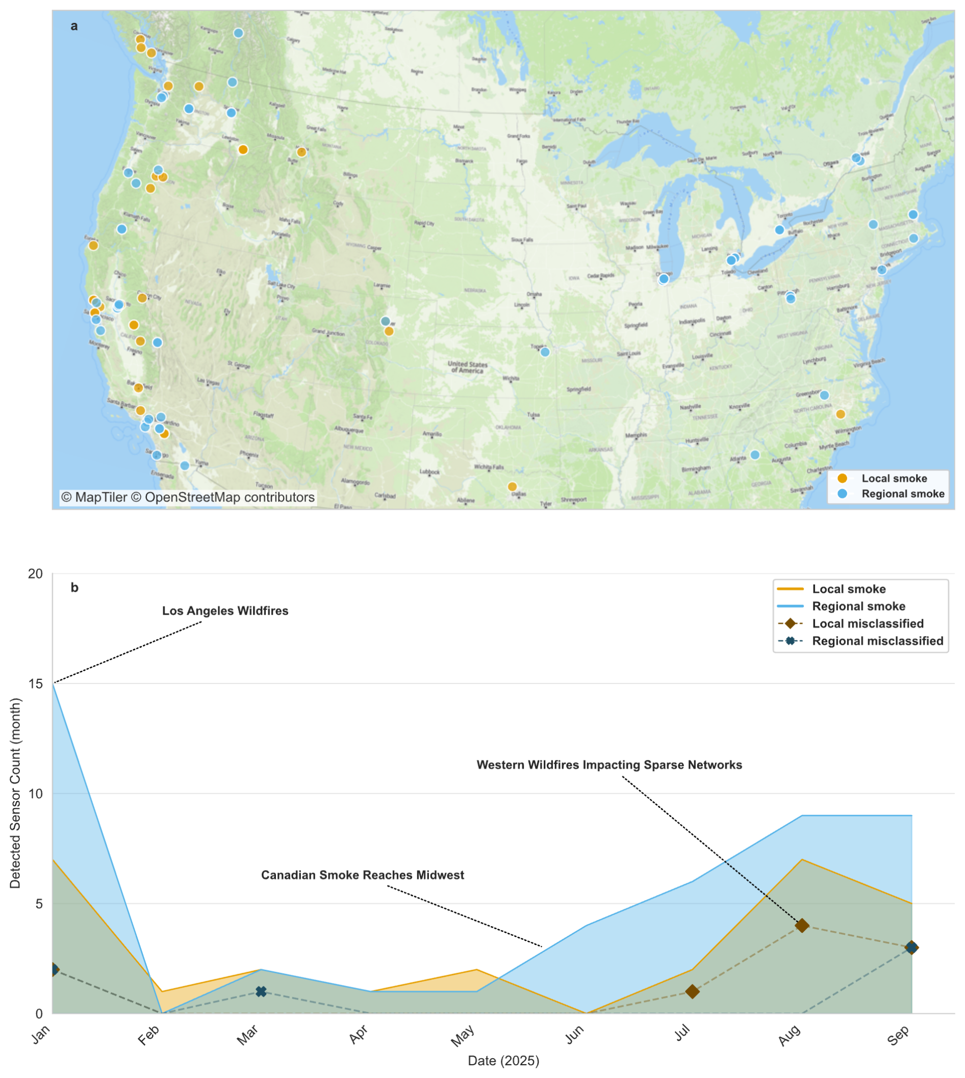
Figure 8 Spatial and temporal distribution of manually validated detections that had an associated smoke event. (a) Geographic locations of local smoke (orange) and regional smoke (blue) events. (b) Monthly counts of manually validated detections, constrained to be unique by both device ID and smoke type to avoid duplicates. Dashed lines indicate misclassifications (false positives). Annotations highlight notable smoke episodes during the study period (January–September 2025). (Basemap: © MapTiler; © OpenStreetMap Distributed under the Open Data Commons Open Database License (ODbL) v1.0; for further information, please see https://www.openstreetmap.org/copyright/en, last access: 14 September 2026.)

Continuing with our cases with persistence>3 h, faulty sensors were more likely to be detected in either the no smoke or regional smoke cases. Within our flagged events with no smoke present, 71 % of flagged events represent genuine sensor malfunctions, rising to 74 % during regional smoke events but dropping to only 11 % during local smoke conditions. This pattern suggests that regional smoke may amplify the detectability of a malfunctioning device, while local smoke events may mask sensor failures or are themselves frequently misclassified as sensor problems. Hyper-local classification shows variation across smoke conditions (11 %–23 % for regional smoke and no smoke; 53 % for local smoke), indicating that truly localized phenomena might be identified regardless of local smoke conditions.

5.4 Hyper-Local Events Versus Faulty Devices

Both outlier detection methods were trained on synthetic measurement signals that arise not only from malfunctioning devices, but also from PM_2.5 conditions that affect only the sensor in question. In reality, the hyper-local events validated in our 9 months of air quality data may be due to siting near a localized emission source (Fig. 9a), indoor placement during a smoke event (Fig. 9b), or other intermittent hardware issues that self-resolve. These events manifest in a single device and may not be representative of ambient air quality relevant to the local population. The distribution of classification type across persistence bins in Table S6 demonstrates both methods' abilities to separate these hyper-local phenomena from truly faulty devices that provide no usable data.

Figure 9 Two examples of persistent hyper-local events from the manual validation. (a) A device deviating from ambient conditions in an extreme way while nearby devices remained unaffected; the event lasted roughly six hours, with four hours flagged by all detection methods. (b) A sensor potentially moved indoors: during a regional smoke event, this privately owned device passed QC checks, but reported significantly muted concentrations compared to its neighbours, and the outlier became apparent only once the network encountered smoke. Colours in the right panels represent EPA AQI category. (Basemap: © MapTiler; © OpenStreetMap Distributed under the Open Data Commons Open Database License (ODbL) v1.0; for further information, please see https://www.openstreetmap.org/copyright/en, last access: 14 September 2026.)

For the information-theoretic method, the first persistence bins with acceptably low misclassification rates are those lasting 3 h or more, where hyper-local events account for ∼76 % of validated detections and device faults remain comparatively uncommon. With more consecutive hours of flagging, the classification shifts decisively: once events persist beyond 13 h, validated cases are overwhelmingly attributed to faulty devices, exceeding 90 %. XGBoost shows the same transition. At 3 h, hyper-local events represent ∼77 % of validated cases with misclassification well below 20 %. But for longer-duration detections beginning around 13 h, faulty devices dominate, rising to $>\mathrm{85}\mathit{\%}-\mathrm{90}\mathit{\%}$ of validated outcomes. Across both methods, these low-misclassification bins exhibit a consistent pattern: short-duration detections are primarily hyper-local phenomena, whereas long-duration detections correspond almost exclusively to a broken or faulty device. By stratifying flagged outliers by their persistence, the methodology provides a practical means of separating hyper-local events from faulty devices.

Broken sensors exhibit significantly lower coefficient of variation (CV=30.5 %, median=11.5 %) compared to hyper-local events (CV=67.6 %, median=52.4 %), reflecting their tendency to report constant or near-constant values. This distinction in time series measurement variability may provide an additional signal for differentiating malfunctioning sensors from hyper-local events, complementing persistence thresholds.

6 Discussion

6.1 Operational Configuration and Tuning Levers

Because fault types are not known in advance, parameters must be chosen without reference to any one of them. Although the best-performing configuration differed by fault type (Sect. 4.1.2), performance was flat near the optimum: under the fixed, method-independent label of Sect. 3.6, at each proximity and binning tested, the configuration that performed best across all fault types scored within 0.014 of each fault type's own optimal F_β=0.5. A practical policy is to tune once across a representative mix of fault types, select the proximity from network density (Sect. 3.1), and match the objective and persistence threshold to the application. The configuration applied at continental scale (Table S5) was set by judgement to be more conservative than this optimum, trading sensitivity to subtle faults for fewer false alarms.

Stratifying detections by persistence offers an operational lever for tailoring how detected outliers may be interpreted and used. For air-quality messaging purposes that prioritize a unified, population-level communication, a lower persistence threshold (e.g., >3 h) may be appropriate. At these durations, a large fraction of hyper-local events and almost all faulty devices may be filtered out while misclassification rates remain very low. This ensures that public messaging reflects regional air-quality conditions rather than transient, sensor-specific anomalies.

For applications that benefit from retaining fine-scale PM_2.5 variability, such as neighbourhood level exposure assessments or high-resolution monitoring, a higher persistence threshold (e.g., >12 h) is more suitable. At this threshold, misclassification is very low, and the vast majority of flagged devices are due to hardware or persistent faults. Configuring parameters and persistence thresholds thus allow this detection framework to be tailored to specific operational contexts, balancing trade-offs between public health messaging and fine-scale PM_2.5 exposure.

Time-series information could be incorporated into the framework fairly simply as well. An additional withhold-classification on a rolling statistic of a device's own record, such as the coefficient of variation over the previous several hours, would defer outlier classification until measurements have somewhat stabilized, complementing the network-based entropy gate and persistence thresholds with an explicitly temporal feature.

6.2 Network Structure, Terrain, and Local Smoke

Defining sensor networks that are appropriately grouped, such that they behave predictably in response to a pollution source, is a significant challenge. Wildland fire events introduce unique smoke regimes that are tightly coupled to fire behaviour, local meteorology, and surrounding topography. As a result, each event produces novel PM_2.5 patterns across a network, and any previously established predictive relationships within networks may become irrelevant under new conditions.

To guard against unwanted outlier flagging, we must consider the sharp gradient that PM_2.5 concentrations may take across a network during a local smoke event, and tune our detection method parameters accordingly. In one local smoke case (Fig. S5), the information-theoretic detections misclassified a valid sensor for 2 consecutive hours due to a nearby fire. To avoid potentially filtering out valid data, we might lower our network entropy threshold, increase our persistence requirements, or leverage the CV on recent measurements, using dynamic behaviour to verify.

Interestingly, the XGBoost method did not classify this event as an outlier; while speculative, this may be the use of antecedent measurement features used in the model, which assess whether a device's recent behaviour is both dynamic and consistent with that of neighbouring sensors. Future work could expand the machine learning training datasets to include either real or synthetic events of this nature that reflect transient smoke that may temporarily create a sharp gradient across a network. It might also be valuable to incorporate additional data sources profiling nearby fire and emissions sources.

Another complication arises when networks are grouped across drainages, which may function as separate airsheds. When the sensor distribution is sparse, imbalanced between drainages, or when the PM_2.5 source is localized, a Euclidean-based distance threshold, such as the one used in this study, may generate disorderly networks. We considered network generation methods that accounted for terrain, and explored the creation of terrain-aware networks using a least-cost path approach (Hart et al., 1968) that used slope as a cost surface. Although this approach increases computational burden and complexity to network generation, early results indicate that these terrain-informed networks exhibit stronger internal consistency among sensors, suggesting improved ability to reduce misclassifications in topographically complex regions.

Figure 10 illustrates this scenario, which shows a network of sensors generated by both methods, using a 7.5 km distance threshold. The primary node was frequently misclassified as an outlier in the winter months, when overnight woodsmoke pollution would settle in the western drainage and remain confined there. The lone sensor in the eastern drainage, left unimpacted, would be flagged using our detection methods if our network was comprised of cross-drainage devices. When terrain is incorporated into network generation, this device's neighbour count is reduced to the single station at the southern end of its own drainage, which appropriately separates the distinct airsheds.

Figure 10 Example of a sensor network in which the primary node was frequently misclassified as an outlier. The left panel shows a network constructed using a Euclidean distance threshold, whereas the right panel shows a terrain-aware network generated using a least-cost path approach with a DEM as the cost surface. This difference in network construction reduces the sensor's neighbour count from 16 to 1, preventing it from being flagged as an outlier in situations where air-quality impacts are confined to the neighbouring drainage. (Basemap: © MapTiler; © OpenStreetMap Distributed under the Open Data Commons Open Database License (ODbL) v1.0; for further information, please see https://www.openstreetmap.org/copyright/en, last access: 14 September 2026. Terrain shading derived from NASADEM (NASA JPL, 2020).)

The elevated misclassification rate during local smoke events reflects how these events are classified, rather than from the correlation length of wildfire smoke in general. Local smoke events were categorized as those where a portion of the network was impacted by smoke, while most of the network was unaffected. Large, transported plumes impact entire networks at once, as wildfire smoke routinely travels regional to continental distances (Zhang et al., 2025), and produces strong network consensus. Smaller sources or sharp plume gradients will impact a network differently. Prescribed and small fires produce less smoke, which disperses over shorter distances and interacts strongly with terrain (Miller et al., 2019). These impact smaller portions of a network, or even individual sensors, making those devices appear anomalous. By construction, local smoke events are therefore the cases in which the network is most disordered, and they represent the hardest classification task for any method performed using a single snapshot in time and built on network agreement. Figure S5 illustrates this regime, with smoke from the nearby Mount Underwood fire impacting part of the Port Alberni network in complex coastal terrain.

6.3 Device Response to PM_2.5 Sources and Sensor Types

The PM_2.5 measurement technologies unique to each device type may respond differently to specific types of particulate sources, particularly when particle size distributions shift toward coarse diameters. Regulatory grade (FEM/FRM) monitors reliably capture PM_2.5 concentrations during both dust storms and wildfire smoke, but many optical sensors common in networks such as PurpleAir (which use the Plantower PMS5003/6003) struggle to properly size and measure larger particles (roughly>1 µm) (Ouimette et al., 2024; Kuula et al., 2020), leading to an underestimation when coarse particles dominate (Jaffe et al., 2023). While steps are being taken towards dust-specific correction algorithms for PMS sensor data (Kaur et al., 2025), this remains a current limitation of our methodology, which assumes a relatively uniform response to particulate matter between network devices. When a majority of sensors in a network share the same Plantower hardware, and a small number of nearby regulatory grade monitors respond correctly to a dust event, the “correct” devices can become outliers (Example Fig. S4). This configuration can undermine methods that rely on neighbourhood agreement. Although this mismatch is less problematic when dust and smoke co-occur, it highlights a fundamental limitation: network-informed detection assumes that sensors and monitors respond similarly to the same pollutant source.

This work evaluated outlier detection on a network of data from permanent monitors, temporary monitors, PurpleAir sensors, SensOR sensors, and SensWA sensors. All devices except for the PurpleAir sensors are solely operated and maintained by air quality experts. Sensors that are not set up by air quality experts may not be sited correctly leading to outlier results because they are located near a hyper-local emission source, the location may not be accurately reported, or the sensor may have been moved inside to understand indoor air quality without updating the location or sensor type. This may have led to many of the issues identified in the operational dataset. There are many other air sensors deployed across the United States with some having similar user deployment methods to PurpleAir. Other networks may have much less frequent siting issues than PurpleAir depending on who and how they are set up.

PurpleAir removes problematic data based on duplicate measurements. SensOR and SensWA sensors also have duplicate sensors to more easily identify issues. Many other sensors on the market do not have duplicate measurements (Barkjohn et al., 2025a) potentially making these outlier detection methods useful for other air sensor types. In addition, different types of sensors may have different common failure patterns than PurpleAir (e.g., repeat zeros, outliers, baseline shift, influences leading to variable relationships with air monitors) (Barkjohn et al., 2025a). They may also have different outlier patterns due to different sampling or averaging intervals (e.g., <1 h sampled for solar devices). These outlier removal methods may perform better or worse for other sensor types depending on their common failure patterns.

Many sensors and monitors have varying uncertainty depending on the measurement type and the concentration range (Agrawal et al., 2025; Khan et al., 2024; Hagler et al., 2022). Sensor response often decreases at high concentration due to saturation or particle coincidence (Agrawal et al., 2025; Kim et al., 2025) and uncertainty can be further influenced by the correction applied to sensor data. The correction applied to PurpleAir sensors in this paper was developed using collocation PM_2.5 data up to 1500 µg m⁻³ and it accounts for nonlinearity above 300 µg m⁻³ (Barkjohn et al., 2022). However, uncertainty may still be higher at these elevated concentration levels compared to lower concentrations, where more training data is available and monitor measurements are more reliable. It is unknown what concentrations range was used in developing the SensWA corrections and it will vary since many different corrections were used. Although a median regression is used for PM_2.5 $\text{data}>\mathrm{100}\mathrm{\mu }\mathrm{g}{\mathrm{m}}^{-\mathrm{3}}$ it is unknown if it will extrapolate accurately to any data outside the concentration range used for correction development and/or if higher concentration data may be underestimated. SensOR use a linear fit so higher concentration data may be underestimated. If we are most interested in AQI category estimation, the highest break point (Very Unhealthy to Hazardous) is 225.5 µg m⁻³. So even if some sensor types underestimate at $\text{concentrations}>\mathrm{225.5}\mathrm{\mu }\mathrm{g}{\mathrm{m}}^{-\mathrm{3}}$, it will not matter for AQI categorization. Variations in correction and uncertainty across concentration ranges may result in differing outlier detection performance among sensor types.

The demonstrated outlier detection framework offers some resilience to these differences through the bin deviation measure D_k shown in Eq. (3) and the flexibility of binning strategy (e.g., the standard AQI, the modified AQI, or custom bin sets). These can be tailored to the variability of a given sensor type or network, particularly at concentration extremes where correction differences are largest, but bin categorization or AQI classification differences are minimal.

6.4 Expanding Machine Learning Applications

Although our machine learning model produced substantial “chatter,” with a high volume of detections overall, and approximately half of the 1 h detections ultimately validated as misclassifications, this behaviour likely reflects limitations in the chosen parameter sets and the perturbation types used in the semi-synthetic training dataset. Retraining the model on a broader context of event types, including human validated events would likely improve classification performance and reduce false positives. Despite these limitations, results in the higher persistence range demonstrate that machine learning models trained on semi-synthetic data can achieve strong performance.

Importantly, the XGBoost methods identified several types of faulty behaviour that the information-theoretic approach could not capture. The models were able to (a) anticipate emerging outliers based on antecedent device behaviour before categorical divergence from neighbouring sensors occurred, and (b) detect problematic signals associated with device malfunction, such as unchanging measurements, implausible variability, or frequent outages. These capabilities suggest that machine learning methods may serve as a more skilful mode of detection when trained on a more comprehensive set of real and synthetic fault scenarios. The capacity of machine learning to leverage a broader and more diverse set of features than our simple rule-based methods is a significant advantage. With quality labelled training data (which requires considerable curation effort), machine learning models could incorporate contextual features, such as nearby fire activity or seasonal patterns, to assess whether flagged readings reflect genuine smoke influence rather than sensor faults or distinguish between hyper-local events and true device faults. However, these capabilities come at the cost of interpretability. Simple equations offer auditable decision logic, whereas machine learning models are less transparent, making them better suited to contexts where explainability is not imperative. Future work should focus on improved training datasets and targeted feature engineering to develop a more robust and generalizable framework than rule-based detection alone can provide.

More sophisticated network methods (Sect. 1) such as GNNs share this dependence on training data, and are reliant on large annotated datasets, which are scarce for sensor faults, and may bias models toward the conditions observed in past events. Time-series foundation models offer a pathway to avoid sensor and network specific training. These models can be applied zero-shot, either to detect anomalies directly from reconstruction error (Goswami et al., 2024) or to supply the forecasts against which residual-based detectors compare (Ansari et al., 2024). In both cases, a measurement is judged against model output, so performance during smoke events depends on predicting the smoke itself. For PM_2.5, zero-shot forecasts fell short of a trained model during California wildfire smoke (Huang et al., 2026), and how zero-shot detectors fare in events like those explored in this paper remains an open question.

We purposely used naive XGBoost models trained on synthetic data to narrow the scope of this study and keep its focus on the tuneable outlier detection equation. It is plausible that, given proper annotation, an XGBoost or more sophisticated machine learning methods trained on real outliers over a larger corpus of data would meaningfully outperform the methods presented here; future work could incorporate the information-theoretic measures developed for sensor networks in this study as features to further such models. We believe there is value in initially exploring large sensor networks through more simplistic and explainable methods. The tuneable equation requires no training data and rests on interpretable quantities that remain visible to the operator, so its behaviour can be changed by adjusting a threshold rather than by re-weighting and re-validating a model.

Physically informed spatiotemporal models offer a complementary path forward. Our networks encode proximity alone, whereas formulations such as the stochastic advection–diffusion model of Choi and Hummel (2025) represent pollutant transport explicitly, and could supply physically grounded expectations of inter-device agreement as a plume moves through a network. Coupling such models with the information-theoretic flags developed here is a natural extension to this work.

7 Conclusions

This work presents a generalizable framework for identifying outlier behaviour in PM_2.5 sensor networks during wildfire smoke events by integrating information-theoretic metrics into both a rule-based equation, as well as a gradient-boosted decision-tree classifier. We applied synthetic perturbations designed to mimic the sensor failures commonly observed in the field to real-world air quality data during 11 different smoke events, demonstrating that an information-theoretic rule-based method can reliably detect statistical outliers with low false-positive rates, while remaining tolerant of the network disorder that occurs during smoke intrusions. Because all comparisons are made in larger, categorical bins on data from monitors and sensors that have been corrected to be comparable, the framework generalizes across device types. We show this methodology complements, not replaces, device-specific calibration and correction. Extending this approach with machine learning features that incorporate short-term dynamics and network-aware behaviour allowed us to capture a broader range of anomalous signatures, including subtle precursor cues and faulty sensor behaviour that may have otherwise gone undetected. When these methods were applied to 9 months of operational data from more than 19 000 devices across the United States and Canada, both approaches showed strong performance in detecting outliers, with accuracy increasing substantially when devices were flagged between consecutive hours. Stratifying devices by their number of consecutive hours being flagged separates outlier types between hyper-local events and sustained sensor malfunctions. This persistence filtering is a practical mechanism for tailoring detection aggressiveness to specific operational contexts: lower thresholds (3+ h) effectively balance precision and recall for applications prioritizing population-level air quality communication, while higher thresholds (12+ h) reliably isolate hardware malfunctions. Extending temporal averaging on measurements, with windows beyond one hour (e.g., 3 h rolling averages), may similarly focus detection on sustained anomalies.

While overall performance was encouraging, this application was intentionally non-prescriptive. The flexibility of both detection approaches, (particularly the tunability of parameter thresholds, persistence criteria, or additional rulesets), means that these tools can be readily adapted to specific operational priorities. For example, the framework could be configured conservatively for regional public-health messaging, where false positives must be minimized, or tuned to retain maximum sensitivity for fine-scale PM_2.5 monitoring in research contexts. Both methods are computationally efficient, requiring minimal processing time per device-hour, and consensus between different parameter sets or binning strategies substantially reduced misclassification rates while adding negligible computational overhead. Future work could expand the representation of real-world fault scenarios, refine network generation methods in complex terrain, and potentially incorporate contextual information such as nearby wildland fire events. These developments could support more reliable automated quality assurance for PM_2.5 sensors, aiding in exposure assessment and supporting public health communication during wildfire smoke and other pollution events.