
the Creative Commons Attribution 4.0 License.
the Creative Commons Attribution 4.0 License.
 | 16 Nov 2026
Characteristics of multiple-trip echoes observed by EarthCARE Cloud Profiling Radar

Takuji Kubota
Hiroaki Horie
Yuichi Ohno
Observations from the EarthCARE Cloud Profiling Radar (CPR) frequently contain spurious cloud signals caused by mirror images, multiple-scattering (MS) tails, and satellite mirror images (SMIs). These multiple-trip echoes are produced when transmitted radar pulses follow longer-than-nominal propagation paths and return within the reception window of subsequent pulses. Distinguishing and removing them is essential for scientific analyses using CPR observations. This study characterizes global properties of the multiple-trip echoes and evaluates the performance of the identification methods implemented in the JAXA Level 2A CPR one-sensor Echo product (CPR_ECO). For mirror images and MS tails, we adopt modelling approaches previously proposed for CloudSat-based analyses, whereas for SMIs we introduce a new method that exploits their characteristic altitude and Doppler-velocity signature associated with line-of-sight satellite-velocity contamination. Evaluations using collocated Atmospheric Lidar (ATLID) measurements, which provide CPR-independent cloud-top information, objectively show that the method properly identifies most of the multiple-trip echoes. Global statistical analyses using the identification flag reveal distinct geographical distributions, seasonal variations, vertical structures, and surface-state-dependent occurrence conditions among the three echo types. Mirror images are the most frequent type, and their distribution broadly follows cloud occurrence, with a preference for ice-free ocean. MS tails are concentrated in tropical and subtropical convective regions under strongly attenuating conditions. In contrast, SMIs occur almost exclusively over surfaces with specular reflection, where the normalized radar cross section is larger than 25 dB, such as melting sea ice and land with surface-water cover. These results provide a basis for improving multiple-trip echo identification and for addressing overlap cases in which spurious echoes contaminate genuine cloud signals.
- Article
(17550 KB) - Full-text XML
- BibTeX
- EndNote


The Earth Cloud Aerosol and Radiation Explorer (EarthCARE) (Illingworth et al., 2015; Wehr et al., 2023; Kubota et al., 2026) satellite was successfully launched on 28 May 2024. The primary objective of EarthCARE is to better understand the effects of clouds and aerosols on the Earth's radiation budget, one of the largest sources of uncertainty in current numerical weather prediction and climate models. To this end, EarthCARE carries four synergistic instruments, namely a radar, a lidar, a multispectral imager, and a broadband radiometer, enabling simultaneous observations of the vertical and horizontal distributions of clouds and aerosols, their particle properties, and their interactions with radiative energy at the top of the atmosphere. The onboard Cloud Profiling Radar (CPR), developed by the Japan Aerospace Exploration Agency (JAXA) and the National Institute of Information and Communications Technology (NICT), is a W-band (94 GHz) nadir-pointing radar. The CPR can extend the climate record of cloud vertical structure established by CloudSat (Stephens et al., 2002), with improved sensitivity (e.g., Xu et al., 2026). Most importantly, the CPR provides the first Doppler velocity measurements from a satellite-borne cloud radar, enabling global observations of cloud dynamics and providing new constraints on particle microphysical properties and vertical air motion (Aoki et al., 2026; Galfione et al., 2025; Kim et al., 2026; Hotta et al., 2026; Roh et al., 2025; Seiki et al., 2025).
The CPR determines the altitude of target hydrometeors from the time delay between the transmission of a radar pulse and the reception of the backscattered signal. However, when the signal follows a longer-than-nominal propagation path owing to processes such as those illustrated in Fig. 1, it is received later than the nominal timing expected for the direct echo path. If the round-trip time of longer path echo exceeds one pulse repetition interval (PRI), the longer path echo appears within observation window and its range is indistinguishable from echoes associated with subsequently transmitted pulses, resulting in range ambiguity. Consequently, the signal is detected as a spurious echo at an aliased altitude determined by the unambiguous range, Ru, given by
where c is the speed of light and PRF is the pulse repetition frequency.
Mirror images are one of the most common spurious echoes in spaceborne radar observations of this kind (Battaglia, 2021; Li and Nakamura, 2002; Meneghini and Atlas, 1986). They represent inverted virtual images of clouds below the surface, formed when the radar signal is reflected by the surface and illuminates the target from below, opposite to the direct path (Fig. 1a). When aliased by Ru, these below-surface images appear in the upper part of the observable range as second-trip echoes. Mirror images have been identified in CloudSat observations (Battaglia, 2021), as well as in Ku- and Ka-band spaceborne radar measurements (Hirose et al., 2023; Li and Nakamura, 2002).
Another type of second-trip echo is the multiple-scattering (MS) tail, which appears as an elongated tail-like echo produced by multiple scattering within deep clouds containing strongly scattering hydrometeors (Fig. 1b). In this case, repeated scattering within the cloud increases the effective propagation path length and delays the return signal, causing the echo to appear at an aliased range (Battaglia and Simmer, 2008). Such MS tails are known to occur frequently in CloudSat observations, particularly in deep convective systems (Battaglia, 2021; Battaglia et al., 2010, 2011).
EarthCARE/CPR measures Doppler velocity using a pulse-pair processing technique, in which Doppler velocities are derived from coherent phase measurements between successive pulses. Such measurements can suffer from Doppler spectrum broadening and velocity aliasing (Hagihara et al., 2023; Kobayashi, 2002; Sy et al., 2014). To mitigate the degradation in Doppler accuracy, EarthCARE/CPR operates at a high pulse repetition frequency (PRF) of 6.1–7.5 kHz, higher than the 3.7–4.4 kHz used by CloudSat. This higher PRF, however, reduces Ru, causing second-trip echoes to be aliased to lower altitudes within the observable range. Battaglia (2021) therefore predicted that such echoes would occur frequently enough to be non-negligible in EarthCARE observations.
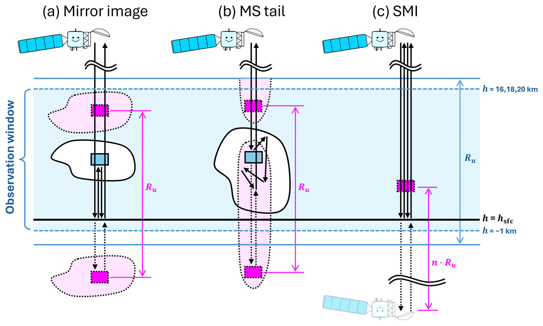
Figure 1Schematic presentation of three types of multiple-trip echoes: (a) mirror images, (b) MS tails, and (c) SMIs. Ru is the unambiguous range and n is the number of pulse repetition intervals (PRIs) between the expected and actual receive windows of the SMI-signal, typically ranging from 17 to 20.
On the other hand, satellite mirror images (SMIs), which had not been anticipated before the launch of EarthCARE, have recently been identified as another type of spurious echo caused by range ambiguity. As illustrated in Fig. 1c, they are artifacts produced when the transmitted radar signal follows a path involving two round trips between the satellite and the surface before being received by the antenna. They appear at altitudes corresponding to the satellite altitude aliased multiple times by Ru, and can therefore be regarded as a form of “multiple-trip” echo. SMIs occur only when surface reflection is extremely efficient, and tend to appear over sea ice in summer and over inland water surfaces. They are also characterized by Doppler velocities that are anomalous compared with those of genuine clouds. The contamination by these echoes, which was not observed by CloudSat, may also be viewed as a consequence of the highly accurate nadir pointing of EarthCARE/CPR, which is designed to minimize Doppler-velocity contamination by horizontal wind components.
Distinguishing and removing these spurious echoes, collectively referred to here as multiple-trip echoes, is essential for cloud analyses using CPR observations. Using EarthCARE/CPR observations, Imura et al. (2026) demonstrated that the occurrence frequency of second-trip echoes caused by mirror images and MS tails depends on latitude and varies among the three CPR observation modes with different PRFs, namely the 16, 18, and 20 km modes. In this study, we characterize the global properties of multiple-trip echoes and evaluate performance of the methods to identify the multiple-trip echoes. The methods for modeling mirror images and MS tails are based on the framework reviewed by Battaglia (2021), whereas a new identification method is introduced for SMIs. Section 2 describes the datasets used in this study. Section 3 presents the identification methods for the three types of multiple-trip echoes, together with their technical background. In Sect. 4, the performance of the identification method is evaluated by comparison with cloud observations from Atmospheric Lidar (ATLID), which is also onboard the EarthCARE satellite. Section 5 presents global statistical analyses based on the identification flag, focusing on the geographical distribution, seasonal variation, and occurrence conditions of multiple-trip echoes in relation to surface condition. Finally, Sect. 6 summarizes the conclusions of this study.
2.1 EarthCARE/CPR
The EarthCARE mission processing chain is summarized by Eisinger et al. (2024). This study documents the technical details and evaluation results of the mirror echo flag in the JAXA L2A CPR one-sensor Echo (CPR_ECO) product version Cc (JAXA, 2024a). The CPR_ECO product uses the L1B CPR one-sensor products (CPR_NOM) as input and provides radar reflectivity factor (Z) and Doppler velocity (V) at horizontal integration lengths of 1 and 10 km, together with signal quality flags and ground-clutter detection. In downstream products, such as JAXA EarthCARE L2A and L2B cloud products (Sato et al., 2025), cloud detection is performed based on the flag information from CPR_ECO.
In the analyses presented in Sects. 4 and 5, we used the mirror echo flag together with the 1 km integrated Z and V. For V, we used values after bias correction (JAXA, 2026; Puigdomènech Treserras et al., 2025) and unfolding correction (Hagihara et al., 2023). Echo occurrence was determined using a threshold of signal to noise ratio larger than −7 dB for the 1 km integrated data. In Sect. 3, the same product was used for illustrative examples, and CPR_NOM version Da or Db (JAXA, 2024b) was additionally used for the analysis related to line-of-sight satellite-velocity contamination in Sect. 3.3.
CPR is operated in three observation modes with different upper boundaries of the observation window: the 16, 18, and 20 km modes (Imura et al., 2026). The 16 km mode uses the highest PRF and therefore provides the highest Doppler-velocity precision, but its smaller Ru makes second-trip echoes more likely to appear at lower altitudes in the observation ranges. In contrast, the 20 km mode uses the lowest PRF and has lower Doppler-velocity precision, but benefits from a larger Ru. The 18 km mode has intermediate characteristics.
EarthCARE products are provided as eight segments per orbit, labeled A–H starting from 22.5° S on the ascending node. For file identification, a “frame” is defined by appending this segment label to the orbit number. For example, frame 01418D in Figure 2 means orbit number 1418 and its fourth segment (67.5–22.5° N).
For the statistical analyses, 20 months of data from August 2024 to March 2026 are utilized. During this period, the use of the three observation modes changed with time. As described in detail by Imura et al. (2026), the 16 km mode was used at higher latitudes, whereas the tropical and subtropical regions were observed in the 20 km mode before 8 July 2025 and in the 18 km mode thereafter. The transition latitude between these regimes was 60° before 26 November 2025 and 40° thereafter.
2.2 EarthCARE/ATLID
ATLID is a High Spectral Resolution LIDAR (HSRL), operating in the ultraviolet spectral domain (355 nm) (Wehr et al., 2023; do Carmo et al., 2021). ATLID provides independent cloud-top information that is not affected by CPR multiple-trip echoes. We used the JAXA EarthCARE L2A ATLID one-sensor Cloud Aerosol product (ATL_CLA) version Cb (Nishizawa et al., 2026; JAXA 2024c), which provides lidar-based masks for clouds and aerosols, as well as backscatter coefficients and extinction coefficients. In this study, ATLID-detected cloud areas were extracted using the target mask in ATL_CLA. For the backscatter signal, we used the 1 km integrated backscattering coefficients, without attenuation correction.
2.3 Surface type classification
Multiple-trip echoes are expected to be related to surface conditions. In Sect. 5, each CPR horizontal grid point was classified according to surface types, namely ice-free ocean, sea ice, snow-covered land, and land with or without surface-water cover. For land-ocean classification, we used the land-ocean mask from the Global Land One-km Base Elevation topographic dataset (GLOBE; Hastings and Dunbar, 1999), which covers the globe on a 30 arcsec grid. The mask was interpolated onto the CPR horizontal grid, namely the Joint Standard Grid (JSG) defined in Eisinger et al. (2024). Sea ice was identified when the sea-ice fraction in the Auxiliary ECMWF Meteorological analysis and forecast fields interpolated onto the JSG (AUX_2D) was greater than zero. Snow-covered land was identified when the snow depth in AUX_2D exceeded 0.01 m of water equivalent.
The presence of surface-water cover over land was determined using the Global Surface Water dataset (GSW; Pekel et al., 2016). Because the distribution of surface water varies seasonally, we used the Monthly Recurrence dataset, which provides the monthly mean recurrence frequency of surface water for the period 1984–2021. The original 30 m data were resampled to a 0.01° grid, and the mean recurrence frequency within each grid cell was defined as the surface-water fraction, fSW. Because GSW is derived from Landsat visible imagery, data are missing in high-latitude regions during polar night. These missing values were replaced by the minimum fSW among months with valid observations. The 0.01° gridded data were then interpolated onto the JSG to assign fSW to each CPR horizontal grid point. In addition, land pixels where the snow depth in AUX_2D exceeded 0.01 m of water equivalent were classified as snow-covered land, assuming that the surface was covered by snow or ice.
2.4 CloudSat-CALIPSO
As a complementary dataset for the discussion, we used observations from the Cloud Profiling Radar (CPR) onboard CloudSat, which is a W-band nadir-pointing spaceborne radar without Doppler capability. CloudSat was launched in April 2006. In Sect. 5.3, we used observations through 2010, before the mission transitioned to daylight-only operations following a battery anomaly. Radar reflectivity and cloud-mask data were obtained from the 2B-GEOPROF R05 product (Marchand et al., 2008), and bins with cloud-mask values of 30 or 40 were classified as clouds.
CloudSat conducted exact nadir-pointing observations with an incidence angle of 0° from 7 July to 15 August 2006, and we analyzed a case observed during this period in Sect. 5.4.2. Ru was calculated using the PRI provided in the CloudSat 1B-CPR product (Tanelli et al., 2008). We also used collocated observations from the Cloud-Aerosol Lidar with Orthogonal Polarization (CALIOP) onboard the Cloud-Aerosol Lidar and Infrared Pathfinder Satellite Observations (CALIPSO; Hunt et al., 2009), specifically the 532 nm attenuated backscattering coefficient from the Level 1B Version 4.10 product (Winker, 2016).
In this section, the identification methods for the three types of multiple-trip echoes are described.
3.1 Mirror images
The method for estimating the echo power of mirror images from direct cloud echoes was presented by Meneghini and Kozu (1990). From the geometrical configuration shown in Fig. 1a, the altitude hm at which the mirror image produced by a hydrometeor target at altitude ht appears as a second-trip echo is given by
where Hsfc is surface elevation. The reflectivity of the mirror image, ZMI (dBZ), is then expressed as follows:
where Hsat is the satellite altitude, k is the specific attenuation, σ0 is the normalized radar cross section, Γ is the Fresnel reflection coefficient of the surface, and θ3dB is the 3 dB beamwidth. The second term represents the difference in the conversion factor from received power to reflectivity associated with the radar range distance. The third term represents the 4-way path integrated attenuation between the hydrometeor target and the surface, which is caused by atmospheric gases or hydrometeors. The last term represents the reduction caused by surface reflection and surface scattering (mirror loss). When ht is very close to the surface, mirror loss is smallest and takes an approximately constant value independent of σ0. As ht increases, the loss becomes larger, whereas it decreases with increasing σ0 (Fig. 1 of Battaglia, 2021). Here, Γ = 0.608, θ3dB=0.095°, and the specific attenuation k (dB km−1) was calculated from reflectivity Z (mm6 m−3) using the empirical relation k=0.0325Z, derived by Protat et al. (2019) from W-band radar observations of tropical cirrus clouds. Figure 2a shows a time-height cross-section of a deep stratiform cloud system observed by the CPR, in which widespread mirror images appear above 15 km altitude. Figure 2b shows the ZMI estimated for the same cross-section using Eq. (3) and it reproduces the spatial pattern of the observed radar reflectivity aloft, Zobs, with a comparable magnitude.
For the identification of mirror echoes, we first calculated the difference between the observed and estimated Z, in dB, as
If the mirror-echo intensity at a given altitude could be estimated perfectly, ΔZMI would be 0 dB, and become negative when the observed echo includes a genuine cloud contribution or when the mirror-image echo is weaker than the background noise level. However, accurate prediction is challenging because of uncertainties in the hydrometeor attenuation, and a variety of scattering properties depending on surface conditions (the third and fourth terms of Eq. 3). We therefore flagged detected echoes at altitudes satisfying ΔZMI(h)>g(h) as likely mirror images. Here, g(h) is an empirically determined altitude-dependent threshold chosen to decrease with height, reflecting the greater likelihood of mirror-image occurrence at higher altitudes. Two thresholds were introduced to indicate two confidence levels, “certain” and “possible”. In CPR_ECO version Cc, , where c0 is a constant set to −20 for the “possible” category and −10 for the “certain” category. Over land, diffuse scattering from rough surfaces causes greater loss of the signal, which leads to an overestimation of ZMI. To account for this effect, g(h) is increased by 20 dB over land. Figure 2c shows the resulting classification, which successfully flags false echoes at high altitudes.
Figure 3a shows the joint histogram of Zobs and ZMI for echoes classified as “certain” mirror images by CPR_ECO during 2025. The slope of the linear regression is close to unity, indicating that the relative variations in echo intensity are well reproduced by the estimate. However, ZMI has a positive bias of 2.67 dB, and most cases fall within approximately dB. This bias may be attributable to an underestimation of losses due to attenuation and surface reflection. For example, the empirical k–Z relationship for stratiform rain at W band is given by k=0.047Z0.94 (Fairall et al., 2018), indicating stronger attenuation than for cirrus clouds. Furthermore, the present calculation uses attenuated Z, resulting in an underestimation. In addition, the loss associated with surface reflection can also be larger than the assumed value because of surface roughness, vegetation, partial water coverage, and roughness of the water surface.
Applying the lower threshold on ΔZMI used in this study reduces the risk of misclassifying strong spurious echoes as genuine cloud echoes, which would be particularly problematic for subsequent cloud analysis. On the other hand, no upper threshold is imposed on ΔZMI, because ZMI can be overestimated owing to the effects described above. Although this criterion may incorrectly classify weak genuine clouds as mirror images, we confirmed that it does not result in excessive removal of true echoes near cloud top in Sect. 4.
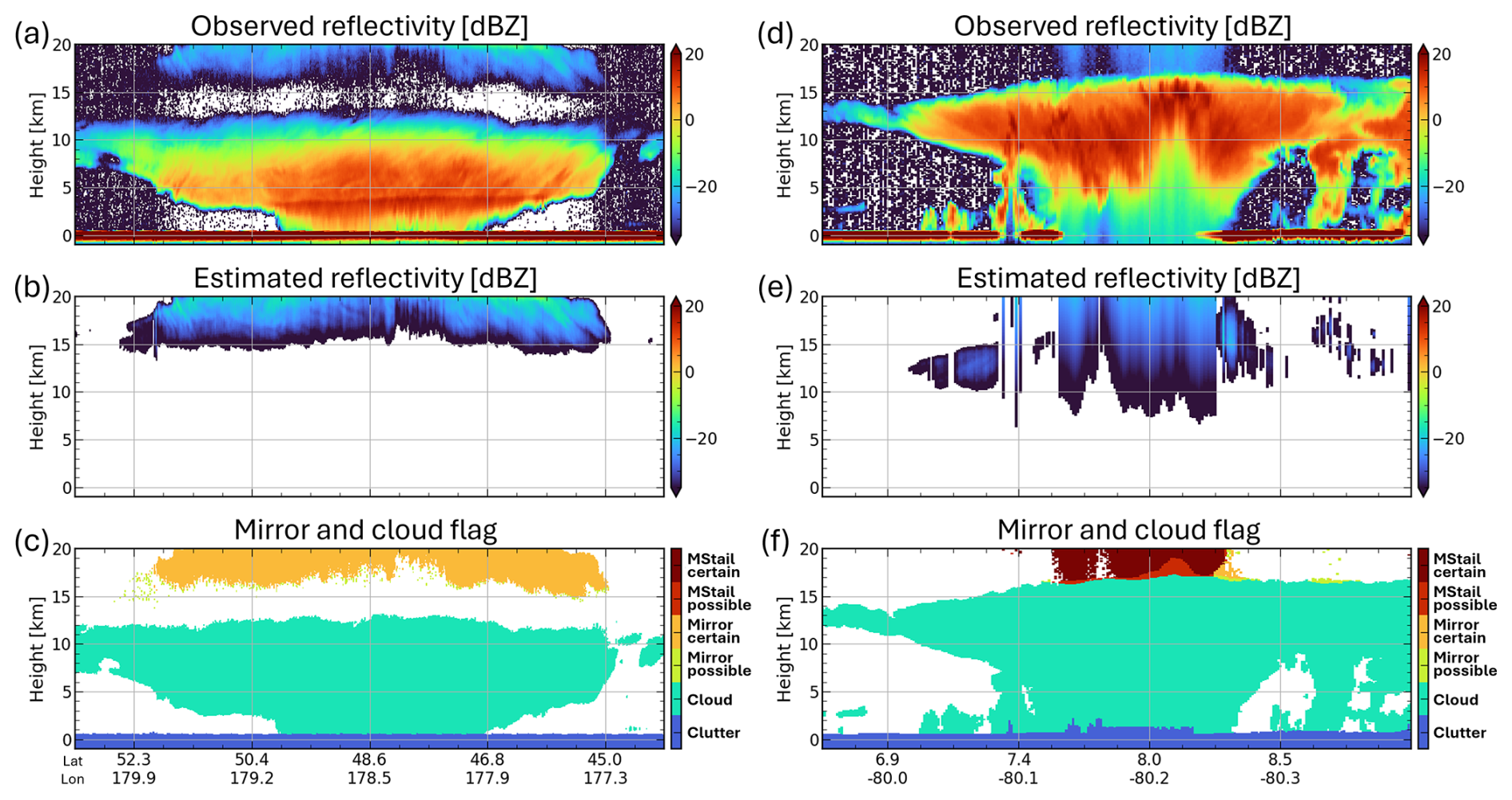
Figure 2Distance-height cross sections of CPR observations for (a–c) a case with prominent mirror images on 28 August 2024 (frame 01418D) and (d–f) a case with prominent MS tails on 16 September 2024 (frame 01717A). Panels (a, d) show the radar reflectivity factor, panels (b, e) show the estimated reflectivity of mirror images (ZMI) and MS tails (ZMStail), and panels (c, f) show the echo-type identification based on the CPR_ECO mirror echo flag.
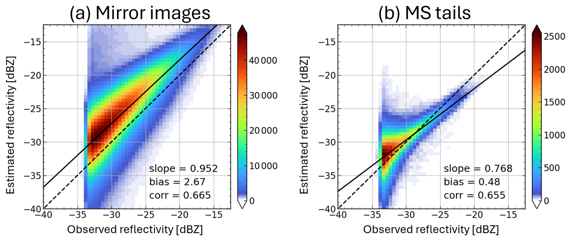
Figure 3Joint histograms of observed and estimated radar reflectivity factor for echoes classified as certain (a) mirror images and (b) MS tails during 2025.
3.2 Multiple-scattering (MS) tails
Figure 2d shows an example of MS tails observed by the CPR. In deep convective clouds, multiple scattering often produces downward-extending tail-like echoes, which are sometimes folded back aloft at the unambiguous range, Ru. Ideally, this phenomenon should be simulated using a 1D radiative transfer code (Hogan and Battaglia, 2008) or more sophisticated Monte Carlo methods (Battaglia and Simmer, 2008). In practice, however, such approaches are limited by their computational cost and by uncertainties in the properties of the scattering particles. As a practical alternative for estimating the MS-induced reflectivity profile, Battaglia (2021) proposed fitting the observed profile with the following function:
where, α, β, and γ are fitting parameters. Above h=hc, the function is exponential, whereas below that level, the function is linear, with a slope equal to that of the exponential function at h=hc, namely c=βγexp(γhc). In this study, c=1.5 dB km−1 and γ=0.25 km−1 were used. Note that hc is introduced empirically to limit the slope and does not necessarily have a unique physical interpretation associated with radar signals or microphysics. During the fitting procedure, data within ±1000 m of the surface elevation were excluded to avoid contamination by surface clutter. The fitted function was then extrapolated and folded at Ru to estimate the echo expected to appear at upper levels.
Figure 2e presents an example of the estimated ZMStail profile. As for the detection of mirror images, the difference between the observed and estimated Z was calculated by , and echoes were flagged according to whether ΔZMStail>g(h) was satisfied. When mirror images and MS tails occurred simultaneously, the larger of the estimated ZMI and ZMStail was used for flagging. Figure 2f shows the resulting classification and demonstrates that the false echoes aloft can be successfully identified. In some areas, the estimated ZMStail extends downward to altitudes where it overlaps with genuine cloud echoes. However, because its intensity is weaker than that of the cloud echo, no flag is assigned in those regions. The histogram shown in Fig. 3b also confirms that the observed and estimated Z values are in reasonable agreement.
3.3 Satellite mirror images (SMIs)
3.3.1 Occurrence altitude
Figure 4 shows an example in which SMIs produce continuous anomalous echoes at a specific altitude over Arctic sea ice in summer. Although their reflectivity is comparable to that of nearby cloud echoes, their Doppler velocities show little spatial variability and exhibit periodic values suggesting an artificial origin. The altitude at which SMIs appear is determined by substituting ht=Hsat in Eq. (2), yielding
The dashed line in Fig. 4a indicates the HSMI altitude estimated from Eq. (6), which agrees well with the observed anomalous echo layers.
When the surface is at sea level, SMIs appear persistently near HSMI=2.4 km. This is because the PRF is controlled as a function of satellite altitude to ensure the required vertical observation range (Imura et al., 2026). Figure 5a and b show the variations in PRF and Hsat over one orbit. Even within the same observation mode, the PRF varies with Hsat.
Figure 6 shows a radar timing diagram of the radar transmission and reception windows, together with the received pulses from the surface and the SMI. Transmission and reception windows alternate, and successive pulses are transmitted in the intervals of PRI before the return from the first transmitted pulse is received. The PRI is controlled according to Hsat so that the return from Earth's ellipsoid (Hsfc=0) is always received Δt(≃16 µs) before the next pulse transmission. The corresponding round-trip travel time, ΔT, therefore satisfies
where n is a positive integer typically ranging from 17 to 20. The SMI pulse travels twice the path length of the first-trip surface echo and is therefore received after a travel time of 2ΔT. Consequently, after the 34th reception timing in this example, the SMI pulse is received Δt earlier than the surface echo from the 18th transmitted pulse. This timing difference corresponds to an apparent altitude of km, explaining why the SMI consistently appears near this altitude.
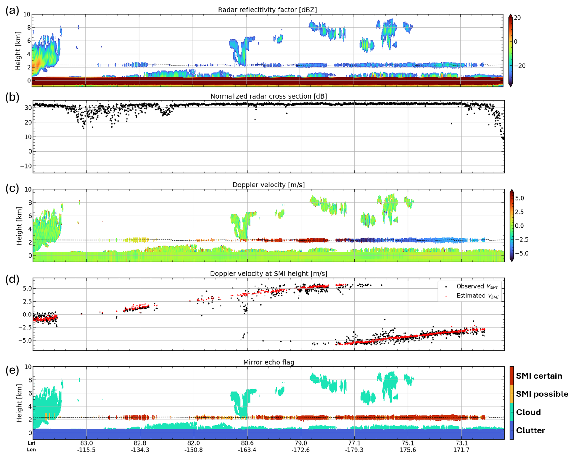
Figure 4CPR observations for a case with prominent SMIs on 4 August 2025 (frame 06725C). Panels (a, c, e) show the vertical cross section of (a) radar reflectivity factor, (c) Doppler velocity, and (e) the echo-type identification based on the CPR_ECO mirror echo flag. Panel (b) illustrates the normalized radar cross section σ0. Panel (d) illustrates the observed and estimated Doppler velocity at HSMI, plotted only where dBZ.

Figure 5(a) PRF; (b) Hsat; and (c) VLOS and expected VSMI calculated assuming Vsfc=0 during one orbit of orbit number 06198 on 1 July 2025.

Figure 6Timing diagrams of the radar transmission and reception windows, together with the received pulses from the surface and the SMI, for an example in the 20 km mode at a satellite altitude of approximately 400 km.

SMIs can also occur over elevated inland water surfaces. Figure 7 shows SMIs generated over the Salar de Uyuni in the Andean Plateau. Because the surface is located at an elevation of approximately 3.7 km, the SMIs appear at about 10 km, as predicted by Eq. (6). Additional echoes suggestive of SMIs are also seen over the foothill region on the left side of the figure, which coincide with the locations of inland water bodies. The strong surface returns may raise the possibility of unanticipated instrumental artifacts associated with receiver saturation, including compression or clipping of the received signal and a possible delayed electronic response. However, the observed echo altitudes are consistent with the predicted SMI geometry, supporting the interpretation that these echoes are generated by the proposed SMI mechanism rather than by a saturation-related instrumental artifact.
3.3.2 Estimation of Z and V for SMIs
In principle, the received power of an SMI echo can be estimated from the radar equation by treating the spacecraft as an effective point target observed through two specular surface reflections:
where Pt is transmitted power, G is the CPR antenna gain at boresight, λ is the wavelength of the radio wave, σsat is the effective radar cross section of the spacecraft, Rsfc is the effective surface reflection factor, and Aatm is the one-way path integrated attenuation. Although Rsfc could be constrained from the first-trip surface echo, this is difficult because the receiver is typically saturated, as indicated by the measured σ0 leveling off at approximately 30 dB (Figs. 4b and 7b). One possible contribution to σsat is structural scattering from the electrically large 2.5 m reflector and other spacecraft components. Another possible contribution is antenna-mode scattering, in which part of the power received by the antenna is reflected at impedance mismatches in the feed system and subsequently reradiated (Munk, 2003; Shrestha et al., 2008). However, the radar cross sections associated with both structural scattering and antenna-mode scattering are unknown, making a more quantitative estimate difficult.
Instead, the Doppler velocity at the SMI altitude, VSMI, can provide a useful diagnostic. The raw Doppler velocity measured by the CPR contains a contribution from the satellite velocity in the line-of-sight direction, VLOS. Because an SMI involves an additional round trip between the satellite and the surface, its Doppler velocity, VSMI, contains an additional VLOS contribution relative to that of the first-trip surface echo as follows:
where VN is the Nyquist velocity. The dominant contribution to VLOS arises from vertical motion of the satellite associated with altitude variations along the orbit (Fig. 5b and c). Its magnitude can reach approximately ±30 m s−1 and can be determined from the satellite telemetry. A smaller contribution to VLOS results from the CPR's antenna beam mis-pointing caused by thermal distortion of the CPR main reflector, uncertainties in the satellite attitude determination, and residual calibration errors (Puigdomènech Treserras et al., 2025). This component also varies systematically over the orbit, but its amplitude is only about 0.3 m s−1.
Ideally, V(Hsfc) would be zero after VLOS-correction. In practice, however, small residual velocities on the order of 0.1 m s−1 remain because of uncertainties in VLOS and variations in surface scattering properties, including effects associated with nonuniform beam filling (NUBF) and the strong incidence-angle dependence of specular reflection. We therefore use the observed V(Hsfc) explicitly rather than assuming it to be zero.
Figures 4d and 7d compare the VSMI predicted from Eq. (9) with the observed Doppler velocity, Vobs(HSMI), demonstrating that the predicted and observed values are in good agreement. In Fig. 4d, the expected and observed VSMI gradually shifts toward more positive velocities from the left to the right side, with folding at VN near 78° N. This feature results from the variation in satellite altitudes as shown in Fig. 5c. Relatively weak noise contamination in VSMI and the corresponding V(Hsfc) may also indicate specular reflection, because only the portion of the radar beam directed very close to the specular direction contributes to the received signal, thereby effectively narrowing the beamwidth.
3.3.3 Identification criteria
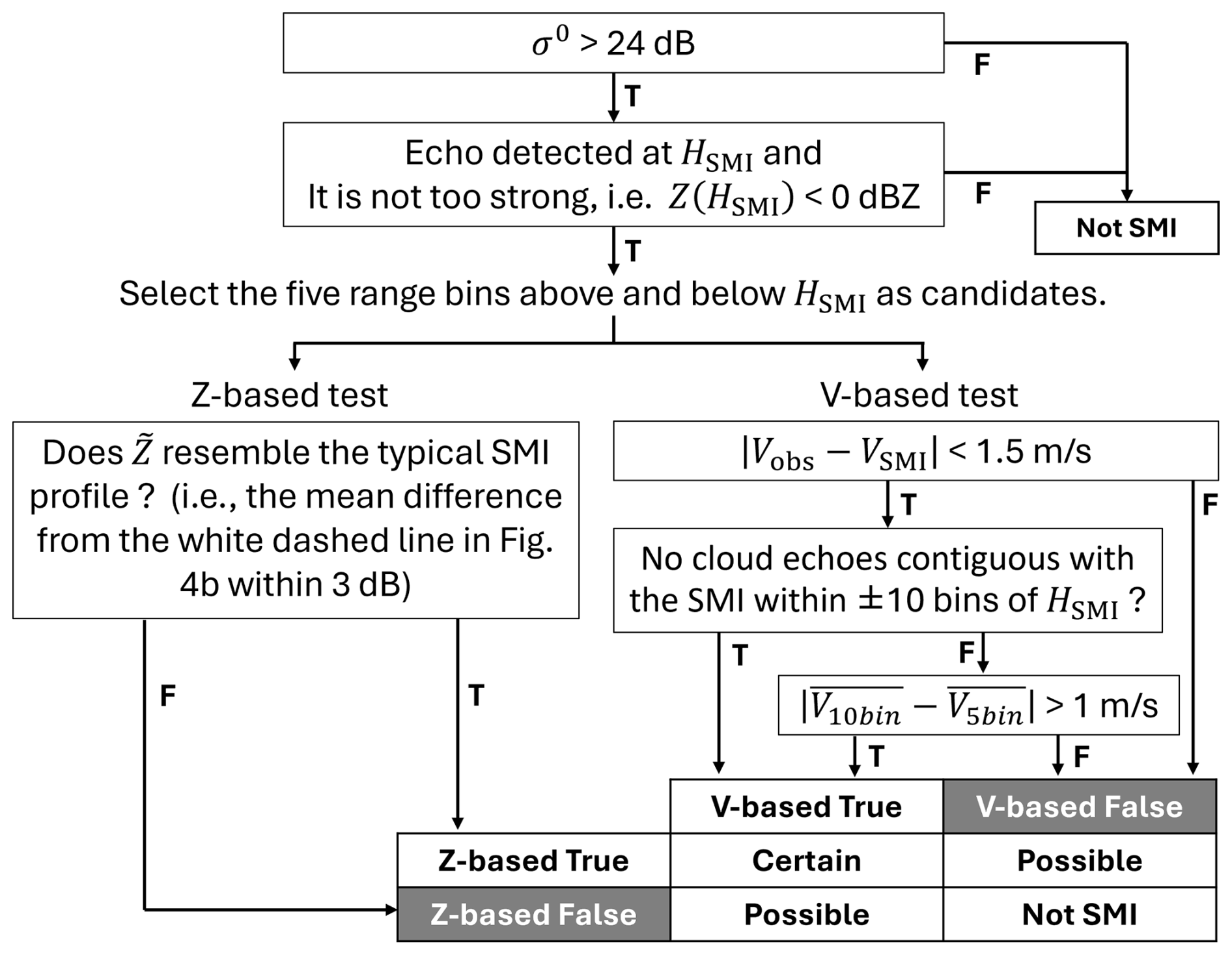
Figure 8 shows contoured frequency by altitude diagrams with relative height, , on the vertical axis. The horizontal axes represent (a) the observed reflectivity, Z(h′), (b) the Z relative to that at HSMI, in dB, , and (c) the difference between the observed Doppler velocity and VSMI, namely . These histograms were compiled from cases in which an echo was detected at h=HSMI. To retain only cases with a high likelihood of SMI occurrence, we selected profiles satisfying σ0>27 dB and having Z(HSMI) higher than the mean Z averaged over the five bins immediately above and below HSMI. At each altitude, the counts were normalized by the total number of observations.
Figure 8a shows that the occurrence frequency of echoes attributed to SMI is concentrated within ±500 m of HSMI, and that most of these echoes are weak, typically below −20 dBZ. The vertical profiles of peak at HSMI and are consistent with the radar's along-range point target response to a strong surface return, as indicated by the white dashed line in Fig. 8b. In addition, Fig. 8c shows that the occurrence frequency of is concentrated around 0 within ±500 m of HSMI, indicating that the VSMI estimated from Eq. (9) agrees well with the observed Doppler velocity of echoes produced by SMI. These results indicate that both the vertical profiles of and the Doppler velocity at HSMI provide useful diagnostics for identifying SMIs.

Figure 8Contoured frequency by altitude diagrams for SMI-detected profiles with height relative to HSMI on the y-axis. The CPR_NOM from August 2024 to June 2025 was used. (a) The observed radar reflectivity (Z), (b) the Z relative to that at HSMI, in dB, and (c) the difference between the observed Doppler velocity and VSMI.
Figure 9 summarizes the detection flowchart developed from the above findings. First, cases with sufficiently strong surface backscatter (σ0>24 dB) are selected. We then select cases in which an echo is detected at HSMI and its reflectivity is not too strong. For the echoes extracted in this way, two tests are applied: one based on Z and the other on V. In the Z-based test, the profile of is compared with the white dashed reference line in Fig. 8b, and only cases with deviations smaller than a prescribed threshold are retained. This step retains only echoes showing the characteristic feature of a peak at HSMI, thereby reducing the risk of misidentifying real cloud echoes as SMIs. In the V-based test, the profile of Vobs is compared with VSMI. If their difference is smaller than a prescribed threshold, the echo is considered consistent with an SMI. However, because VSMI can occasionally be close to Vobs of real clouds, an additional comparison is made with Vobs of the surrounding contiguous echoes. Only cases in which this difference exceeds a threshold are identified as SMIs. Finally, by combining the Z-based and V-based tests, the confidence level is assigned as “certain” when both tests are satisfied, whereas the level is assigned as “possible” when only one test is satisfied.
Collocated ATLID measurements provide cloud detections that are unaffected by the multiple-trip echo problem that occurs in CPR observations. Therefore, by examining whether the cloud-top heights (CTHs) derived from the two instruments are consistent, we can assess whether clouds are being properly removed in the CPR algorithm. Figure 10 shows an example of CPR and ATLID observations of a stratiform precipitation system over the midlatitude ocean. Because ATLID signals are strongly attenuated within clouds, ATLID cannot observe the internal cloud structure. However, it can detect upper-level clouds, especially ice clouds, with higher sensitivity than CPR. Therefore, the ATLID-derived cloud top height (CTHATL) is generally expected to be at the same altitude as, or higher than, the CPR-derived cloud top height (CTHCPR). In this case, however, CPR echoes are observed above the ATLID cloud top, clearly suggesting the presence of second-trip echoes, which are produced here by mirror images. The shading in Fig. 10c represents the multiple-trip echo identification flag produced from CPR-only information by the CPR_ECO mirror echo flag. The flagged region is consistent with the ATLID cloud top, indicating that the spurious echoes are appropriately identified.
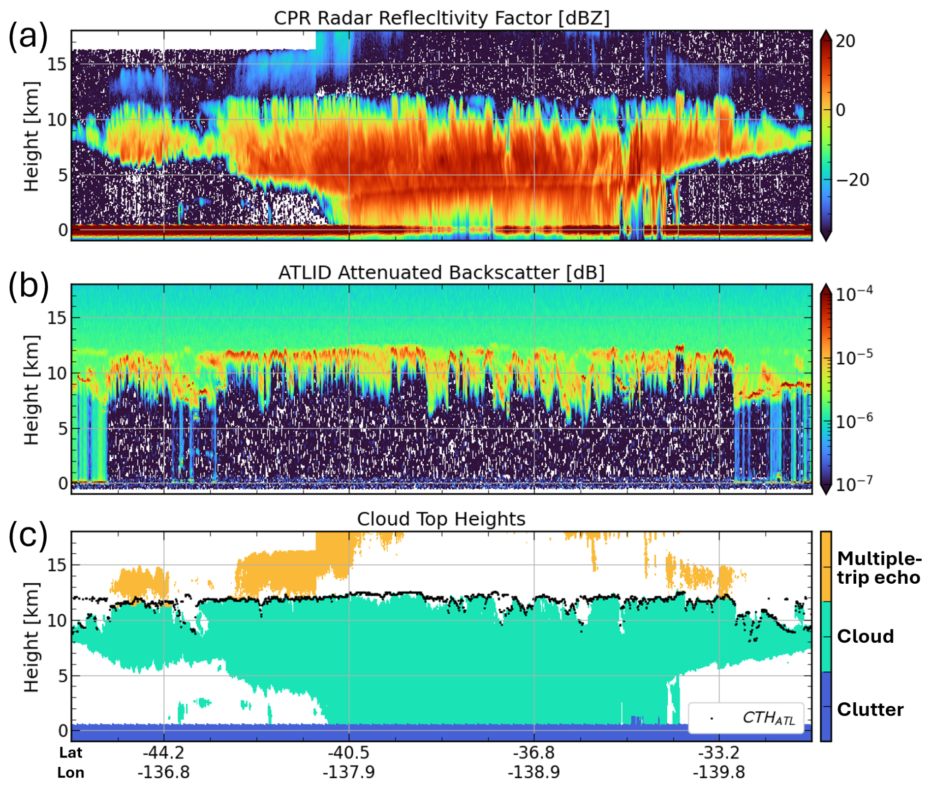
Figure 10Vertical cross-sections of CPR and ATLID observations for a case on 16 February 2026 (frame 09779H). (a) CPR radar reflectivity factor, (b) ATLID attenuated backscattering coefficients, (c) CPR cloud identification mask with ATLID-derived cloud top heights in black dots.
To evaluate the validity of the identification scheme of multiple-trip echoes, we performed a statistical analysis based on ATLID-derived CTHs. Figure 11 shows joint histograms of CPR and ATLID CTHs, accumulated over 20 months of data from August 2024 to March 2026. In Fig. 11a and b, the vertical axis represents CTHCPR before the removal of multiple-trip echoes, whereas Fig. 11c shows CTHCPR after their removal. Figure 11b is identical to Fig. 11a except that the color scale is logarithmic.
As shown in Fig. 11a and b, the CTHCPR and CTHATL mostly lie along the one-to-one line, indicating generally good agreement. However, there are distinct frequency maxima concentrated near 16, 18, and 20 km independent of the value of CTHATL. The three altitudes correspond to the upper boundaries of the three observation modes, and these correspond to cases erroneously identified as cloud top because of second-trip echoes due to mirror images and MS tails. In addition, CTHCPR shows a frequency peak near 2.5 km regardless of CTHATL. This altitude corresponds to the expected height of SMIs when the surface is near sea level, indicating that SMI artifacts are sometimes misidentified as cloud tops. After flag application, these artificial peaks, both at high altitudes and near 2.5 km, are largely suppressed in Fig. 11c, confirming that the multiple-trip echo artifacts are successfully removed.

Figure 11Joint histograms of ATLID-derived (CTHATL) and CPR-derived cloud top heights (CTHCPR). The vertical axis in (a, b) represents CTHCPR before the removal of multiple-trip echoes, whereas the vertical axis in (c) represents CTHCPR after their removal. The counts are normalized by the total number of observations. Panel (b) is identical to panel (a) except that the color scale is logarithmic.
On the other hand, Fig. 11b also shows a small number of cases below the one-to-one line, where CTHATL is higher than CTHCPR. In particular, when CTHATL exceeds 14 km, CTHCPR remains mostly around 12–16 km, almost independently of CTHATL. These cases are dominated by optically thin ice clouds that are detected by ATLID but remain below the detection sensitivity of CPR. They may also include cases in which aerosols are misclassified as clouds in the ATL_CLA product. Conversely, there are also cases in which CTHCPR is higher than CTHATL. These may include cases in which the ATL_CLA product classifies clouds as aerosols or as “unknown” targets, as well as situations in which the W-band radar detects cloud tops at higher altitudes than the lidar in the lower to middle troposphere, as reported by Hagihara et al. (2014). Although outside the scope of this study, such radar-lidar discrepancies may provide useful information on the properties of optically thin particles aloft and could contribute to future improvements in particle property retrieval algorithms.
Figure 12 shows profiles of the CPR echo fraction for each CTHATL bin, separated by the 16, 18, and 20 km observation modes. The red solid line in each panel indicates the lowest altitude at which mirror images can appear, assuming that the ATLID cloud top coincides with the true CPR cloud top. This altitude is calculated from Eq. (2) with Hsfc=0 using the maximum PRF for each observation mode: 7500, 7150, and 6550 Hz for the 16, 18, and 20 km modes, respectively. Before flag application (Fig. 12a–c), echoes are observed in the region above both the red line and the black one-to-one line, where mirror images are expected to appear as second-trip echoes, with frequencies about one order of magnitude lower than those of genuine cloud echoes. After flag application, these echoes are removed, as shown in Fig. 12d–f.
The apparent tendency for second-trip echoes to extend more frequently into the lower troposphere in the 18 km mode (Fig. 12b) than in the 16 km mode (Fig. 12a) is primarily attributable to the different latitude bands in which the two modes are operated (Imura et al., 2026). The 18 km mode is used at lower latitudes and therefore includes observations of tropical deep clouds, allowing second-trip echoes to appear at lower apparent altitudes. In contrast, the 16 km mode is operated only at higher latitudes, where cloud tops are generally lower and the corresponding second-trip echoes remain at higher altitudes.
In Fig. 12b and c, the CTHATL ranges in which second-trip echoes show frequency maxima exhibit a bimodal structure, with peaks at approximately 5–13 and 14–17 km. These two peaks are associated with mirror images and MS tails, respectively. This suggests that, for deep clouds with high cloud tops, strong attenuation suppresses the occurrence of mirror images, whereas MS tails become more likely to occur. The lack of a distinct MS-tail peak in Fig. 12a can be explained by the fact that MS tails are primarily confined to tropical regions, as discussed in Sect. 5, while the 16 km mode has been used only poleward of 40°. A more detailed comparison of the second-trip echo occurrence among observation modes is provided by Imura et al. (2026).
Furthermore, Fig. 12b and c indicate that second-trip echoes are sometimes connected to the upper parts of clouds rather than being clearly separated from them, although their occurrence frequency is low and is visually emphasized by the logarithmic scale. Even in such cases, the spurious echoes are identified in a manner broadly consistent with CTHATL, without excessive removal of genuine cloud echoes. However, when CTHATL exceeds 14 km, CPR tends to identify the cloud top at a lower altitude because of its lower sensitivity (Fig. 11). Therefore, a more detailed assessment of how well the method separates spurious echoes from genuine cloud echoes in such cases, mainly those involving MS tails, remains a subject for future work.

Figure 12Mean vertical profiles of the CPR echo fraction for each CTHATL bin (a–c) before and (d–f) after the flag application. Results are shown for the three observation modes: (a, d) 16 km, (b, e) 18 km, and (c, f) 20 km mode. Red lines indicate the lowest altitude at which mirror images can appear, assuming that the ATLID cloud top coincides with the true CPR cloud top.
5.1 Geographical location and seasonal variations
To characterize the geographical and seasonal distributions of multiple-trip echoes in EarthCARE/CPR observations, we performed a statistical analysis for the period from August 2024 to March 2026 using the mirror echo flag. Figure 13 presents annual-mean maps of the occurrence frequency for each echo category, namely all echoes, clouds, mirror images, MS tails, and SMIs, together with the frequency of strong CPR surface backscatter (σ0>24 dB), sea-ice occurrence, and land surface water occurrence. A column was classified as containing a given echo type when that echo was detected in at least five bins (∼500 m). Because a simple average over all observations would be affected by month-to-month differences in the number of samples, the annual mean was calculated after normalizing by the number of observations in each month so that all months contributed equally.

Figure 13Maps of annual-mean occurrence frequency for each echo category: (a) all echo types, (b) clouds, (c) mirror images, (d) MS tails, and (e) SMIs, as well as the frequency of (f) strong CPR surface backscatter with σ0>24 dB, (g) sea-ice occurrence, and (h) inland-water occurrence.
Among the three types of multiple-trip echoes, mirror images (Fig. 13c) show the highest occurrence frequency. Their spatial distribution closely resembles that of cloud occurrence (Fig. 13b), with frequent appearances over the tropics and along the midlatitude storm tracks. Mirror images also tend to occur more frequently over the ocean than over land, consistent with the higher surface reflectivity of the ocean. On the other hand, they are absent over the subtropical eastern ocean basins, where low-level clouds dominate, because mirror images associated with low-cloud-top clouds do not reach the second-trip observation window. Figure 14 presents 3 month seasonal-mean zonal averages for each echo type for December–February (DJF), March–May (MAM), June–August (JJA), and September–November (SON), together with the occurrence frequency of strong surface backscatter. The seasonal migration of mirror images in Fig. 14c is consistent with the north-south shifts of the Intertropical Convergence Zone (ITCZ) and the midlatitude storm tracks seen in Fig. 14a. Their occurrence frequency is higher in the Southern Hemisphere midlatitudes, where the ocean-covered area is larger.
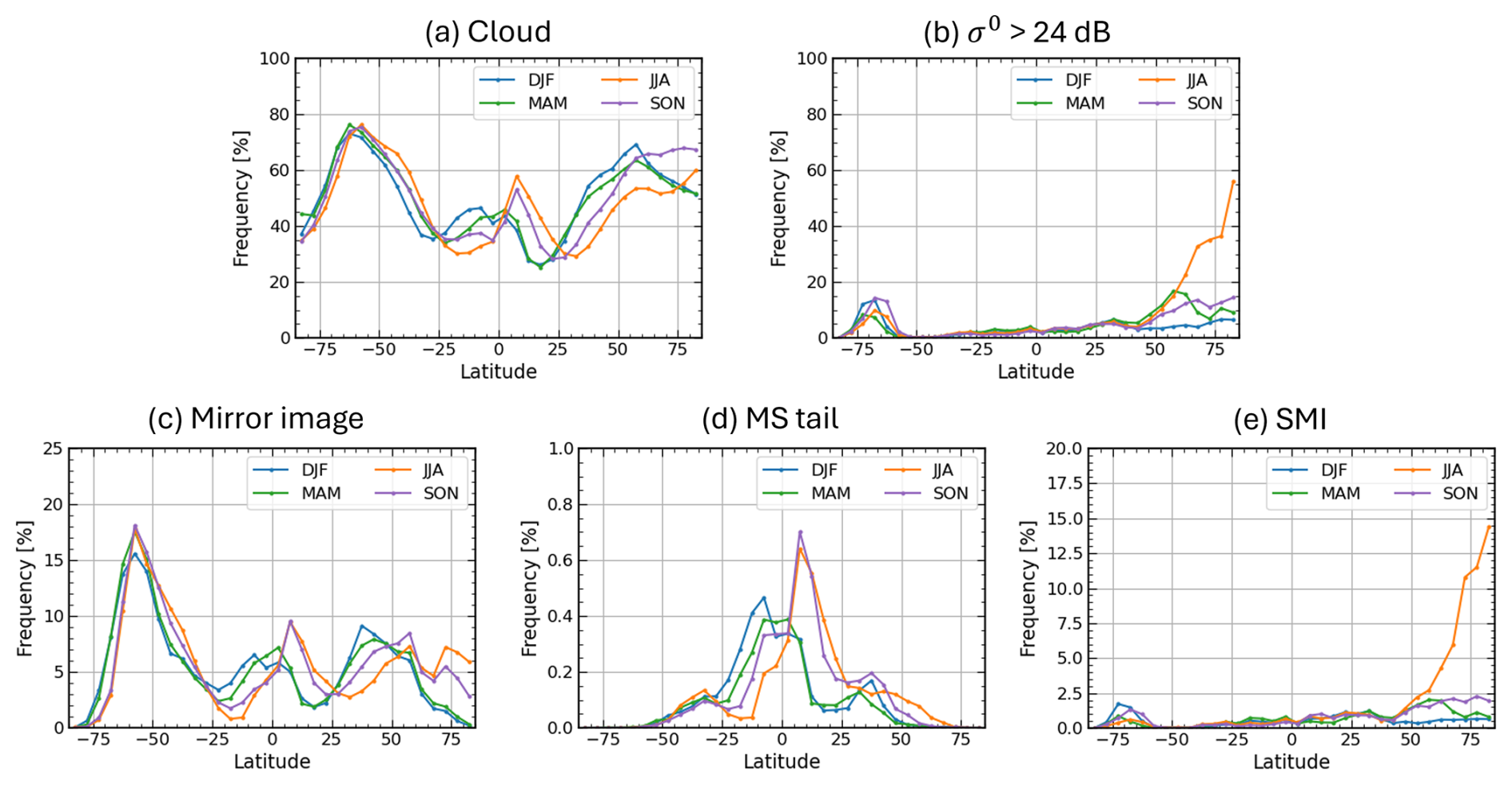
Figure 14Latitudinal dependence of the seasonal mean occurrence frequency of (a) clouds, (b) strong CPR surface backscatter with σ0>24 dB, (c) mirror images, (d) MS tails, and (e) SMIs. Each line indicates 3 month averages for December–February (DJF), March–May (MAM), June–August (JJA), and September–November (SON).
MS tails occur less frequently than mirror images and exhibit a more scattered spatial distribution, with no clear land-ocean contrast (Fig. 13d). They are most frequent in the tropics, particularly around the Maritime Continent and along the ITCZ, suggesting a close correspondence with the distribution of deep convection. The seasonal evolution shown in Fig. 14d is also consistent with the seasonal migration of cloud occurrence in the tropics shown in Fig. 14a.
Whereas mirror images and MS tails occur only in the presence of clouds, regions with a high occurrence frequency of SMIs are independent of cloud occurrence and instead correspond closely to regions of strong surface backscatter (Fig. 13e and f), as expected from their generation mechanism (Fig. 1c). These regions coincide well with sea-ice-covered areas in the Arctic Ocean and along the Antarctic coast, as well as inland areas covered by water surfaces such as major rivers, lakes, and wetlands. This spatial correspondence suggests that SMIs are generated by specular reflection of the transmitted radar pulses at the smooth surface. As shown in Fig. 14b and e, surface backscatter over sea ice is often particularly strong during summer when surface melting or refreezing is likely to occur, and the occurrence frequency of SMIs is enhanced in the corresponding seasons. Unless these SMIs are properly removed, cloud occurrence frequency would be overestimated, causing the apparent distribution to resemble that shown in Fig. 13a rather than the true distribution shown in Fig. 13b.
5.2 Dependence on surface conditions
The previous section suggested that the occurrence of each echo type is linked to distinct surface conditions. In this section, we further clarify these relationships through an analysis stratified by σ0 and surface type. Figure 15 shows the dependence on σ0 of (a) the number of observations and (b) the relative occurrence frequency for each echo type, and (c) the probability density function (PDF) for each surface type. The relative occurrence frequency is defined as the number of occurrences of a given echo type divided by the total number of observations for each σ0 value. As described in Sect. 2, surface type is classified into six categories: ice free ocean, sea ice, snow-covered land, and land with surface-water fraction (fSW) of 0 %, 0 %–50 %, and > 50 %. Note that the σ0 used here is not corrected for attenuation. Therefore, in the presence of attenuation by precipitation or other hydrometeors, the observed σ0 can be lower than the value expected from the intrinsic surface properties.
The attenuated σ0 distributions of the number of observations and the number of detected cloud echoes in Fig. 15a exhibit two distinct peaks, around 5–10 dB and around 30 dB, respectively. These peaks correspond to differences in the reflective properties of the underlying surface types. The former peak coincides with the peak in the σ0 PDF for ice-free ocean, which covers a large portion of the globe, and is also close to the PDF peaks over land without surface water and over snow-covered land. In contrast, the latter peak corresponds to the PDF peak over land with surface-water cover (fSW>0). This secondary peak arises from receiver saturation in the CPR, whereby surface backscatter stronger than the saturation level is recorded near that level, approximately 29 dB before 26 November 2024 and approximately 32 dB after the Signal Processing Unit was switched from the redundant system to the nominal system (Imura et al., 2026). Sea ice shows a bimodal σ0 PDF. The peak near 5 dB is similar to that for snow-covered land, suggesting that diffuse scattering by snow particles dominates in these cases. By contrast, the other peak near 30 dB is likely associated with specular reflection from sea-ice surfaces undergoing surface melting or refreezing during summer.

Figure 15The dependence on σ0 of (a) the number of observations and (b) the relative occurrence frequency for each echo type, namely all echo types, clouds, mirror images, MS tails, and SMIs. (c) The dependence on σ0 of the probability density function (PDF) for each surface type, namely ice-free ocean, sea ice, snow-covered land, and land with surface-water fraction (fSW) of 0 %, 0 %–50 %, and > 50 %. σ0 is not corrected for attenuation.
The distribution of mirror images is also bimodal, similar to that of cloud echoes (Fig. 15a). In the σ0 range of 0–10 dB, which corresponds to the primary maximum in occurrence frequency, the relative occurrence frequency of mirror images is about 5 % or higher. A second maximum appears near σ0∼30 dB, where the relative occurrence frequency of mirror images is particularly high, reaching 10 %–80 %. In contrast, the occurrence frequency is low at low σ0 values ( dB). This is likely because the transmitted radar pulse is strongly attenuated by hydrometeors along the four-way path between the target and the surface (the third term in Eq. 3), such that little energy remains to be reflected back to the CPR antenna. Figure 16 shows the fractional distribution of surface types for cases in which each echo type was detected. Compared with cloud echoes, mirror images occur preferentially over ice-free ocean (87 %), consistent with the peak at moderate σ0 values shown in Fig. 15. Over land, the fraction of cases without surface-water cover is substantially smaller for mirror images than for cloud echoes. This is likely attributable to the inefficient reflection of the transmitted radar pulse from rough land surfaces, that is, to small values of Γ in Eq. (3).

Figure 16The fractional distribution of surface types for all observations and for cases in which each echo type was detected. The surface-type classification is the same as that used in Fig. 15c.
MS tails occur preferentially at low σ0, with a relative occurrence frequency of about 5 % for dB. This is consistent with the fact that attenuation is also strong in the types of clouds in which multiple scattering typically occurs, such as deep convection. The surface type at the time of occurrence is predominantly ocean, accounting for about 80 % of the cases, suggesting that the amount of inland surface water is not a major controlling factor. Because MS tails are concentrated mainly in the tropics, they are not observed over sea ice or snow-covered land.
Figure 15a shows that SMIs occur only at high σ0 as inferred in the previous section. In particular, when σ0 is near the saturation level of about 30 dB, their relative occurrence frequency reaches approximately 20 %–60 %, which is comparable to that of genuine cloud echoes. The discontinuity in the frequency distribution at 24 dB in Fig. 15a arises because a lower threshold in σ0 is imposed in the classification procedure (Fig. 9). The surface-type distribution associated with SMI occurrence is also distinct from those of the other echo types, with sea ice and land with surface-water cover being the dominant categories because they can produce near-saturated σ0 values (Figs. 15c and 16).
5.3 Zonal mean latitude-height distributions
Figures 17a–o show zonal-mean height distributions of echo occurrence frequency, mean radar reflectivity factor, and mean Doppler velocity for each echo category, namely all echoes, clouds, mirror images, MS tails, and SMIs, averaged over the 7 month period from December 2024 to June 2025. During this analysis period, the latitude separating the observation modes remained unchanged, with the 20 km mode operated equatorward of 60° latitude and the 16 km mode poleward of 60°. Cloud echoes were defined as echoes that were not classified as any type of multiple-trip echo. In addition, to exclude residual second-trip echoes that may have been missed by the flag, suspected echoes more than 500 m above CTHATL and above the lowest possible mirror-image altitude were excluded. The lowest possible mirror-image altitude was calculated for each observed profile in the same manner as the red line in Fig. 12. Note that echo occurrence frequency (the first column in Fig. 17) is displayed on a logarithmic scale, so even very low occurrence frequencies appear visually enhanced.
The occurrence frequency of mirror images is higher than that of the other types of spurious echoes. Its vertical distribution resembles an upside-down version of the cloud echo fraction, suggesting that, as anticipated by Battaglia (2021), there are cases in which mirror images overlap with genuine clouds at altitudes around 12–16 km. Although the echo fraction of MS tails is smaller than that of mirror images, they also extend into altitude ranges in the tropics where genuine clouds are present, suggesting the possibility of overlap.
It should be noted that the present analysis is based on a binary classification according to the presence or absence of the flag, and therefore does not include cases in which mirror images overlap with actual clouds. In particular, the lower boundary of the mirror-image frequency distribution is fixed at around 12 km between approximately 30° S and 30° N. In reality, however, mirror images in the tropics may extend to lower altitudes, which implies that the true occurrence frequency of mirror images may be underestimated.
The mean reflectivity of mirror images and MS tails is typically around −30 to −25 dBZ, which is weaker than that of genuine clouds at the same altitude (Fig. 17h and k). However, near cloud top in latitude bands where overlap between genuine clouds and second-trip echoes is suspected, the mean reflectivity reaches values around −20 dBZ, higher than in latitude bands without such overlap (Fig. 17b). This suggests that the second-trip echo signal may be superimposed on genuine cloud echoes.
Figure 17p and q show the cloud echo fraction and mean reflectivity observed by CloudSat, averaged over the corresponding months from 2007 to 2010. They are closely consistent with those from EarthCARE/CPR (Fig. 17d and e), indicating that statistical properties of clouds can be reasonably reproduced when second-trip echoes are properly removed. The more frequent echo occurrence and lower mean reflectivity observed by EarthCARE compared with CloudSat are consistent with the higher sensitivity of EarthCARE/CPR, whose minimum designed detectable reflectivity is approximately −35 dBZ, compared with approximately −29 dBZ for CloudSat.
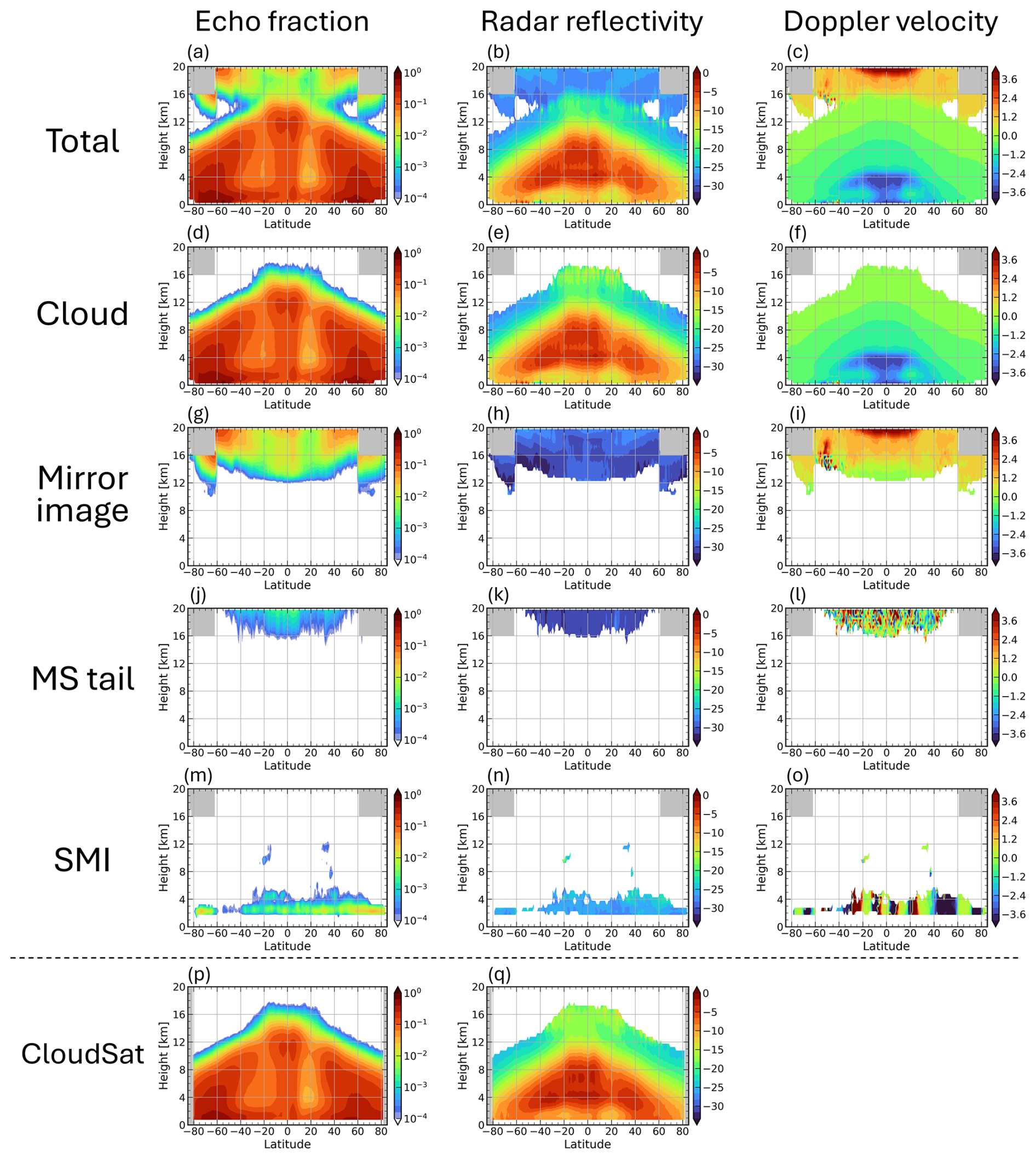
Figure 17(a–o) Zonal-mean height distributions of echo occurrence frequency, mean radar reflectivity factor, and mean Doppler velocity for each echo category, namely all echoes, clouds, mirror images, MS tails, and SMIs observed by EarthCARE/CPR, averaged over the 7 month period from December 2024 to June 2025. (p, q) Zonal-mean height distributions of echo occurrence frequency and mean radar reflectivity factor observed by CloudSat averaged over the corresponding months from 2007 to 2010.
Above 15 km in the tropics, the mean reflectivity is anomalously large, reaching approximately −15 dBZ compared with that at midlatitudes in both Fig. 17e and q. This may be because, in deep convective systems extending to altitudes of 15–17 km in the tropics, relatively large ice particles are transported into the upper troposphere, resulting in enhanced radar reflectivity at these altitudes (Field et al., 2007; Yuan et al., 2011). For EarthCARE, however, the contribution of second-trip echoes cannot be completely excluded. In overlapping cases, the power of second-trip echoes may be superimposed on genuine cloud echoes, or weak cloud-top echoes may be masked by second-trip echoes, causing only relatively strong echoes to be identified as clouds. As shown in Fig. 3, the estimated reflectivity of second-trip echoes still involves considerable uncertainty. Further improvement in the estimation of second-trip echo and subtraction of its contribution from the observed reflectivity would therefore be desirable for better treatment of such overlapping cases.
The primary occurrence altitude of SMIs is approximately 2.5 km, which is consistent with the altitude expected over the ocean at sea level from Eq. (6). In some regions at northern and southern midlatitudes, SMIs are also identified at elevated altitudes (Fig. 17m). These cases originate from lakes or flooded salt flats over high-terrain regions such as the Tibetan Plateau and the Andes. The mean reflectivity of SMIs is around −25 to −20 dBZ comparable to that of clouds (Fig. 17n), so they may be misidentified as shallow stratiform clouds if they are not properly removed.
The Doppler velocities of multiple-trip echoes exhibit distinct characteristics depending on the echo type. Since mirror images of the cloud are obtained by the reflected radar power from the surface, the Doppler velocity of a mirror image signal becomes opposite sign to the direct cloud echo. Under the assumption of perfect nadir pointing, the Doppler velocity of mirror images, VMI, is therefore given by
Consistent with this, the vertical distribution in Fig. 17i is approximately the sign-reversed counterpart of that for direct cloud echoes. In contrast, the Doppler velocity in bins affected by MS tails, VMStail, appears essentially random because it arises from multiple scattering (Fig. 17l). The Doppler velocity of SMIs depends on the line-of-sight satellite-velocity contamination, VLOS, as given by Eq. (9). Because VLOS includes the apparent upward and downward motion of the surface during the satellite orbit, SMI Doppler velocity exhibits a clear latitudinal dependence (Fig. 17o). These distinct Doppler-velocity signatures are potentially useful not only for identifying SMIs, for which Doppler velocity is already included in the classification criteria (Fig. 9), but also for detecting mirror images and MS tails. This suggests that further improvements in the detection scheme could be achieved by making use of Doppler-velocity information.
5.4 Incidence angle dependence of SMIs
5.4.1 Zero Doppler observation of EarthCARE/CPR
If the occurrence of SMI echoes is indeed associated with specular reflection at the surface, even a slight off-nadir pointing of the CPR beam should suppress their occurrence. During a one-day period from 15 to 16 November 2024, covering 16 orbits (frames 02652G–02668F), a special operation referred to as the “Zero Doppler” observation was conducted. In this mode, the spacecraft attitude was controlled so that the CPR beam remained perpendicular to the satellite velocity vector. This operation was designed to minimize VLOS, but consequently caused the beam direction to deviate from the local surface normal. We therefore examined whether the occurrence of SMIs was reduced during this period.
Figure 18a and d show global maps of SMI occurrence frequency during the Zero Doppler observations and during the subsequent 16 nominal orbits (frames 02668G–02684F), respectively. The occurrence frequency of SMIs is clearly lower during the Zero Doppler observations than during the nominal observations. Figure 18b and e show maps of the CPR beam incidence angle relative to the WGS84 Earth ellipsoid, averaged over the respective period, while Fig. 18c and f show their zonal mean values. Under nominal observations, the incidence angle is generally on the order of 0.01°, indicating the CPR beam is closely aligned with the local surface normal. In contrast, the incidence angle during the Zero Doppler observations exhibits a clear latitudinal dependence. The latitude bands in which SMIs are observed in Fig. 18a broadly correspond to regions where the incidence angle is smaller than approximately 0.05–0.1°. Since the 3 dB beamwidth of the CPR is approximately 0.095°, SMIs are expected to occur preferentially when the incidence angle is smaller than roughly half of the 3 dB beamwidth, or approximately 0.05°. The results shown in Fig. 18 are consistent with this expectation and provide further evidence supporting the proposed SMI-mechanism.

Figure 18Maps of (a, d) SMI occurrence frequency and (b, e) CPR beam incidence angle on the Earth ellipsoid, together with (c, f) the zonal mean incidence angle, for the Zero Doppler observations (frame 02652G–02668F) and the subsequent nominal observations (frame 02668G–02684F).
5.4.2 CloudSat's nadir pointing observation
The occurrence conditions of SMIs discussed above suggest that similar echoes can also occur in other spaceborne radars. CloudSat conducted nadir-pointing observations with an incidence angle of 0° from 7 July to 15 August 2006. To avoid receiver saturation associated with specular surface reflection, the pointing direction was subsequently changed to 0.16° off nadir on 15 August 2006. Figure 19 shows a CloudSat observation over the Arctic Ocean on 1 August 2006, during the period of exact-nadir observations. An echo is observed near 5.5–6 km, indicated by the dashed line, where an SMI is expected to appear according to Eq. (6). At the same time, σ0 reaches a plateau near 25 dB, suggesting that the receiver reached saturation due to specular reflection at the surface. No corresponding signal is observed in the 532 nm backscatter measured by the CALIPSO lidar, confirming that the radar echo is spurious rather than a genuine cloud echo. Unlike for EarthCARE, the expected SMI altitude in CloudSat is not constant because its PRF is controlled differently from the scheme described in Eq. (7). These results confirm that SMIs are not unique to EarthCARE and can also occur in other nadir-pointing spaceborne radars when the condition for specular surface reflection is satisfied.

Figure 19CloudSat (a) radar reflectivity factor and (b) σ0, together with (c) the CALIPSO lidar 532 nm attenuated backscatter coefficient, during CloudSat nadir observations on 1 August 2006 (orbit 01389).
In EarthCARE/CPR observations, multiple-trip echoes generated by mirror images, multiple-scattering (MS) tails, and satellite mirror images (SMIs) occur frequently. Distinguishing these echoes from genuine clouds is therefore an essential prerequisite for scientific analyses using CPR observations. This study presents a robust methodology for identifying these three types of false echoes, implemented as the mirror echo flag in the JAXA Level 2A CPR one-sensor Echo product (CPR_ECO). The performance of the method was evaluated through comparison with collocated cloud-top height observations from the ATLID. The results demonstrate that most of the mirror images and MS tails are removed, and that apparent SMIs are also properly identified and screened out. Furthermore, global statistical analyses using this flag reveal distinct type-dependent characteristics in the geographical distributions, vertical distribution, and seasonal variations.
For second-trip echoes, namely mirror images and MS tails, Battaglia (2021) proposed modeling methods based on CloudSat observations and emphasized their importance for EarthCARE, whose higher PRF is required as a trade-off for its Doppler capability. In this study, we implemented these methods and demonstrated that they are highly effective for identifying these echoes. We also introduced a new identification method for SMIs, which were not observed by CloudSat but appear in EarthCARE/CPR observations as a consequence of its highly accurate nadir pointing. Because SMIs typically occur at an altitude of approximately 2.4 km, they can be difficult to distinguish from genuine clouds using reflectivity-based criteria alone. We therefore showed that their Doppler velocity can be estimated from the surface Doppler velocity by accounting for satellite velocity contamination in line-of-sight, and incorporated this information into the identification procedure to make the method more robust.
Collocated ATLID measurements provide cloud-top heights that are independent of CPR and unaffected by the multiple-trip echo problem. The objective evaluation of the CPR identification method using CTHATL demonstrated that most second-trip echoes caused by mirror images and MS tails are appropriately removed. In addition, the artificial frequency maximum of CTHCPR near 2.5 km, which is caused by SMIs, is also eliminated, confirming that SMIs are successfully screened out. This framework provides a basis for evaluating future refinements of the flag and for quantifying the frequency with which multiple-trip echoes overlap with genuine clouds. Although outside the scope of this study, the properties and distributions of clouds detected by ATLID but missed by CPR, as well as the converse cases reported at low to mid-levels in the CloudSat era by Hagihara et al. (2014), are also worthy of future investigation.
The statistical analyses showed that the geographical distributions, seasonal variations, and vertical structures differ among echo types, and that these differences are closely related to surface conditions associated with their respective generation mechanisms. Mirror images, the most frequent type of multiple-trip echo, exhibit spatial distributions that closely resemble those of clouds. They occur preferentially over ice-free ocean, where surface backscatter is stronger than over land, but occur less frequently when attenuation by precipitation is strong. MS tails are less frequent than mirror images, but their distribution resembles that of clouds in the tropical and subtropical regions, and they occur preferentially under strongly attenuating conditions with dB. SMIs exhibit a distinct dependence on surface properties, occurring only for σ0 values above approximately 25 dB, approaching the CPR receiver saturation level of approximately 30 dB. Their occurrence is strongly concentrated over sea ice affected by summer surface melting and over land with surface-water cover. Analysis of the special observation period with slightly off-nadir pointing showed that SMIs occurred only when the incidence angle relative to the local surface was smaller than approximately half of the CPR beamwidth, supporting the interpretation that their occurrence is associated with specular reflection at the surface. SMIs were also identified during the period when CloudSat operated at exact nadir. These results suggest that SMIs are not unique to EarthCARE/CPR and may occur in other nadir-pointing spaceborne radars when the conditions are satisfied.
On the other hand, the current identification method sometimes leaves second-trip echoes at high altitudes. This is likely because the estimation of mirror-image intensity is sometimes unsuccessful owing to uncertainties in the attenuation by hydrometeors and in the surface return efficiency. Another remaining limitation is that identification alone cannot fully address cases in which multiple-trip echoes overlap with genuine cloud echoes. Exploiting the distributional characteristics of each echo type, their relationships with surface conditions, and the statistical properties of Doppler velocity shown in Sect. 5 may help reduce these uncertainties. These constraints could support further refinements of the flagging procedure and, ultimately, enable estimation of the contaminated reflectivity and Doppler velocity in overlap cases.
A promising direction for future work is to develop methods for removing multiple-trip echoes from CPR observations using synergistic products from both the CPR and ATLID. Further improvements may also be achievable for CPR-only products, for example through machine-learning approaches trained with collocated ATLID observations.
All EarthCARE products (https://doi.org/10.57746/EO.01jdvd0xm10ema4rxwbpcd0dn1, JAXA, 2024a; https://doi.org/10.57746/EO.01jdvcydwjf63vpdbjp, JAXA, 2024b; https://doi.org/10.57746/EO.01jkwjk45jrx9frz6c11, JAXA, 2024c) used in this study can be downloaded from the JAXA G-Portal. The multiple-trip echo identification flag used in this study is available as the mirror echo flag in CPR_ECO version Cb and later. The CloudSat products (1B-CPR; 2B-GEOPROF) used in this study have been downloaded from the CloudSat Data Processing Center.
The supplement related to this article is available online at https://doi.org/10.5194/amt-19-7445-2026-supplement.
SA developed the identification method for multiple-trip echoes, implemented it in the CPR_ECO product, carried out the data analysis, and prepared the initial draft of the manuscript. TK, HH, and YO contributed to the development of the identification method, interpretation of the results, and preparation of the manuscript.
The contact author has declared that none of the authors has any competing interests.
Publisher's note: Copernicus Publications remains neutral with regard to jurisdictional claims made in the text, published maps, institutional affiliations, or any other geographical representation in this paper. The authors bear the ultimate responsibility for providing appropriate place names. Views expressed in the text are those of the authors and do not necessarily reflect the views of the publisher.
This article is part of the special issue “Early results from EarthCARE (AMT/ACP/GMD inter-journal SI)”. It is not associated with a conference.
The authors thank the members at ESA-JAXA EarthCARE Joint Mission Advisory Group (JMAG) and Quality Working Group (QWG). We are grateful to Dr. Kaya Kanemaru for suggesting the possibility that the spurious echoes observed near 2.5 km originate from satellite mirror images. This paper was edited for English language quality using an AI-based tool.
This work was supported by JST, ARiSE, Japan (grant no. JPMJAR2639).
This paper was edited by Hajime Okamoto and reviewed by two anonymous referees.
Aoki, S., Kubota, T., and Turk, F. J.: Exploring vertical motions in convective and stratiform precipitation using spaceborne radar observations: insights from EarthCARE and GPM coincidence dataset, Atmos. Meas. Tech., 19, 79–100, https://doi.org/10.5194/amt-19-79-2026, 2026.
Battaglia, A.: Impact of second-trip echoes for space-borne high-pulse-repetition-frequency nadir-looking W-band cloud radars, Atmos. Meas. Tech., 14, 7809–7820, https://doi.org/10.5194/amt-14-7809-2021, 2021.
Battaglia, A. and Simmer, C.: How does multiple scattering affect the spaceborne W-band radar measurements at ranges close to and crossing the sea-surface range?, IEEE Trans. Geosci. Remote Sens., 46, 1644–1651, https://doi.org/10.1109/TGRS.2008.916085, 2008.
Battaglia, A., Tanelli, S., Kobayashi, S., Zrnic, D., Hogan, R. J., and Simmer, C.: Multiple-scattering in radar systems: A review, J. Quant. Spectrosc. Radiat. Transf., 111, 917–947, https://doi.org/10.1016/j.jqsrt.2009.11.024, 2010.
Battaglia, A., Augustynek, T., Tanelli, S., and Kollias, P.: Multiple scattering identification in spaceborne W-band radar measurements of deep convective cores, J. Geophys. Res., 116, https://doi.org/10.1029/2011jd016142, 2011.
do Carmo, J. P., de Villele, G., Wallace, K., Lefebvre, A., Ghose, K., Kanitz, T., Chassat, F., Corselle, B., Belhadj, T., and Bravetti, P.: ATmospheric LIDar (ATLID): pre-launch testing and calibration of the European Space Agency instrument that will measure aerosols and thin clouds in the atmosphere, Atmosphere, 12, 76, https://doi.org/10.3390/atmos12010076, 2021.
Eisinger, M., Marnas, F., Wallace, K., Kubota, T., Tomiyama, N., Ohno, Y., Tanaka, T., Tomita, E., Wehr, T., and Bernaerts, D.: The EarthCARE mission: science data processing chain overview, Atmos. Meas. Tech., 17, 839–862, https://doi.org/10.5194/amt-17-839-2024, 2024.
Fairall, C. W., Matrosov, S. Y., Williams, C. R., and Walsh, E. J.: Estimation of Rain Rate from Airborne Doppler W-Band Radar in CalWater-2, J. Atmos. Oceanic Technol., 35, 593–608, https://doi.org/10.1175/JTECH-D-17-0025.1, 2018.
Field, P. R., Heymsfield, A. J., and Bansemer, A.: Snow Size Distribution Parameterization for Midlatitude and Tropical Ice Clouds, J. Atmos. Sci., 64, 4346–4365, https://doi.org/10.1175/2007JAS2344.1, 2007.
Galfione, A., Battaglia, A., Puigdomènech Treserras, B., and Kollias, P.: First insights into deep convection by the Doppler velocity measurements of the EarthCARE Cloud Profiling Radar, Atmos. Meas. Tech., 18, 6747–6763, https://doi.org/10.5194/amt-18-6747-2025, 2025.
Hagihara, Y., Okamoto, H., and Luo, Z. J.: Joint analysis of cloud top heights from CloudSat and CALIPSO: new insights into cloud top microphysics, J. Geophys. Res.-Atmos., 119, 4087–4106, https://doi.org/10.1002/2013JD020919, 2014.
Hagihara, Y., Ohno, Y., Horie, H., Roh, W., Satoh, M., and Kubota, T.: Global evaluation of Doppler velocity errors of EarthCARE cloud-profiling radar using a global storm-resolving simulation, Atmos. Meas. Tech., 16, 3211–3219, https://doi.org/10.5194/amt-16-3211-2023, 2023.
Hastings, D. A. and Dunbar, P. K.: The global land one-kilometer base elevation (GLOBE) digital elevation model, version 1.0, NOAA National Geophysical Data Center, Boulder, CO, USA, available at: http://www.ngdc.noaa.gov/mgg/topo/globe.html (last access: 10 November 2026), 1999.
Hirose, M., Okada, K., Kawaguchi, K., and Takahashi, N.: Removing interfering signals in spaceborne radar data for precipitation detection at very high altitudes, J. Atmos. Ocean. Technol., 40, 969–985, https://doi.org/10.1175/JTECH-D-22-0114.1, 2023.
Hogan, R. J. and Battaglia, A.: Fast lidar and radar multiple-scattering models. Part II: Wide-angle scattering using the time-dependent two-stream approximation, J. Atmos. Sci., 65, 3636–3651, https://doi.org/10.1175/2008JAS2643.1, 2008.
Hotta, H., Suzuki, K., Kikuchi, M., Aoki, S., and Kubota, T.: Characteristics of tropical clouds with strong updrafts revealed by Doppler-velocity measurements from EarthCARE/CPR, Atmos. Chem. Phys., 26, 11605–11626, https://doi.org/10.5194/acp-26-11605-2026, 2026.
Hunt, W. H., Winker, D. M., Vaughan, M. A., Powell, K. A., Lucker, P. L., and Weimer, C.: CALIPSO lidar description and performance assessment, J. Atmos. Oceanic Technol., 26, 1214–1228, https://doi.org/10.1175/2009JTECHA1223.1, 2009.
Illingworth, A. J., Barker, H. W., Beljaars, A., Ceccaldi, M., Chepfer, H., Clerbaux, N., Cole, J., Delanoë, J., Domenech, C., Donovan, D. P., Fukuda, S., Hirakata, M., Hogan, R. J., Huenerbein, A., Kollias, P., Kubota, T., Nakajima, T., Nakajima, T. Y., Nishizawa, T., Ohno, Y., Okamoto, H., Oki, R., Sato, K., Satoh, M., Shephard, M. W., Velázquez-Blázquez, A., Wandinger, U., Wehr, T., and van Zadelhoff, G.-J.: The EarthCARE satellite: The next step forward in global measurements of clouds, aerosols, precipitation, and radiation, Bull. Am. Meteorol. Soc., 96, 1311–1332, https://doi.org/10.1175/BAMS-D-12-00227.1, 2015.
Imura, Y., Aoki, S., Kubota, T., Nakatsuka, H., Ohno, Y., and Okamoto, H.: Observation modes of EarthCARE/CPR with different Doppler measurement accuracy: evaluation of their applicability, Atmos. Meas. Tech., 19, 5617–5631, https://doi.org/10.5194/amt-19-5617-2026, 2026.
JAXA: EarthCARE/CPR L2A CPR one-sensor Echo Product, JAXA [data set], https://doi.org/10.57746/EO.01jdvd0xm10ema4rxwbpcd0dn1, 2024a.
JAXA: EarthCARE/CPR L1B CPR one-sensor Received Echo Power Products and Doppler Product, JAXA [data set], https://doi.org/10.57746/EO.01jdvcydwjf63vpdbjp0vz6v64, 2024b.
JAXA: EarthCARE/ATLID L2A ATLID one-sensor Cloud Aerosol Products, JAXA [data set], https://doi.org/10.57746/EO.01jkwjk45jrx9frz6c11x4rs8e, 2024c.
JAXA: EarthCARE JAXA Level 2 Algorithm Theoretical Basis Document (L2 ATBD), JAXA, https://www.eorc.jaxa.jp/EARTHCARE/document/doc_index_e.html (last access: 12 May 2026), 2026.
Kim, J., Tan, I., Kollias, P., Puigdomènech Treserras, B.: First EarthCARE CPR Observations of dynamics–microphysics coupling in marine cold-air outbreak clouds, Geophys. Res. Lett., 53, e2025GL121514, https://doi.org/10.1029/2025GL121514, 2026.
Kobayashi, S.: A unified formalism of incoherent, quasi-coherent, and coherent correlation signals on pulse-pair Doppler operation for a cloud-profiling radar: Aiming for a space mission, J. Atmos. Ocean. Technol., 19, 443–456, https://doi.org/10.1175/1520-0426(2002)019<0443:AUFOIQ>2.0.CO;2, 2002.
Kubota, T., Kikuchi, M., Muto, M., Hashimoto, M., Imura, Y., Maruyama, K., Hoffmann, A., Hummel, T., Koopman, R., Malina, E., Rusli, S., Tzallas, V., von Bismarck, J., and Frommknecht, B.: Summary of the EarthCARE Science and Validation Workshop 2025 – Early achievements and future perspectives for the Earth Cloud Aerosol and Radiation Explorer (EarthCARE) satellite mission, J. Eur. Meteorol. Soc., 100037, https://doi.org/10.1016/j.jemets.2026.100037, 2026
Li, J. and Nakamura, K.: Characteristics of the mirror image of precipitation observed by the TRMM precipitation radar, J. Atmos. Ocean. Technol., 19, 145–158, https://doi.org/10.1175/1520-0426(2002)019<0145:COTMIO>2.0.CO;2, 2002.
Marchand, R., Mace, G. G., Ackerman, T., and Stephens, G.: Hydrometeor Detection Using Cloudsat – An Earth-Orbiting 94-GHz Cloud Radar. J. Atmos. Oceanic Technol., 25, 519–533, https://doi.org/10.1175/2007JTECHA1006.1, 2008.
Meneghini, R. and Atlas, D.: Simultaneous ocean cross section and rainfall measurements from space with a nadir-looking radar, J. Atmos. Ocean. Technol., 3, 400–413, https://doi.org/10.1175/1520-0426(1986)003<0400:SOCSAR>2.0.CO;2, 1986.
Meneghini, R. and Kozu, T.: Spaceborne Weather Radar, Artech House, Norwood, MA, 208 pp., ISBN 978-0890063828, 1990.
Munk, B. A.: Finite Antenna Arrays and FSS, John Wiley & Sons, Hoboken, New Jersey, USA, https://doi.org/10.1002/0471457531, 2003.
Nishizawa, T., Kudo, R., Oikawa, E., Higurashi, A., Jin, Y., Sugimoto, N., Sato, K., and Okamoto, H.: Algorithms to retrieve aerosol optical properties using lidar measurements on board the EarthCARE satellite, Atmos. Meas. Tech., 19, 729–744, https://doi.org/10.5194/amt-19-729-2026, 2026.
Pekel, J.-F., Cottam, A., Gorelick, N., and Belward, A. S.: High-resolution mapping of global surface water and its long-term changes, Nature, 540, 418–422, https://doi.org/10.1038/nature20584, 2016.
Protat, A., Rauniyar, S., Delanoë, J., Fontaine, E., and Schwarzenboeck, A.: W-Band (95 GHz) Radar Attenuation in Tropical Stratiform Ice Anvils, J. Atmos. Ocean. Technol., 36, 1463–1476, https://doi.org/10.1175/JTECH-D-18-0154.1, 2019.
Puigdomènech Treserras, B., Kollias, P., Battaglia, A., Tanelli, S., and Nakatsuka, H.: EarthCARE's cloud profiling radar antenna pointing correction using surface Doppler measurements, Atmos. Meas. Tech., 18, 5607–5618, https://doi.org/10.5194/amt-18-5607-2025, 2025.
Roh, W., Satoh, M., Matsugishi, S., Aoki, S., Kubota, T., and Okamoto, H.: Vertical motions in clouds from EarthCare satellite and a global storm-resolving modeling, Sci. Rep., 16, 2622, https://doi.org/10.1038/s41598-025-32256-8, 2025.
Sato, K., Okamoto, H., Nishizawa, T., Jin, Y., Nakajima, T. Y., Wang, M., Satoh, M., Roh, W., Ishimoto, H., and Kudo, R.: JAXA Level 2 cloud and precipitation microphysics retrievals based on EarthCARE radar, lidar, and imager: the CPR_CLP, AC_CLP, and ACM_CLP products, Atmos. Meas. Tech., 18, 1325–1338, https://doi.org/10.5194/amt-18-1325-2025, 2025.
Seiki, T., Horie, H., Hagihara, Y., Aoki, S., and Noda, A. T.: Global identification of dominant ice-particle growth in cirrus clouds using EarthCARE satellite observations, EGUsphere [preprint], https://doi.org/10.5194/egusphere-2025-4819, 2025.
Shrestha, S., Balachandran, M. D., Agarwal, M., Zou, L.-H., and Varahramyan, K.: A method to measure radar cross section parameters of antennas, IEEE T. Antenn. Propag., 56, 3494–3500, https://doi.org/10.1109/TAP.2008.2005541, 2008.
Stephens, G. L., Vane, D. G., Boain, R. J., Mace, G. G., Sassen, K., Wang, Z., Illingworth, A. J., O'connor, E. J., Rossow, W. B., Durden, S. L., Miller, S. D., Austin, R. T., Benedetti, A., and Mitrescu, C.: The cloudsat mission and the a-train, B. Am. Meteor. Soc., 83, 1771–1790, https://doi.org/10.1175/BAMS-83-12-1771, 2002.
Sy, O. O., Tanelli, S., Takahashi, N., Ohno, Y., Horie, H., and Kollias, P.: Simulation of EarthCARE Spaceborne Doppler Radar Products Using Ground-Based and Airborne Data: Effects of Aliasing and Nonuniform Beam-Filling, IEEE Trans. Geosci. Remote Sens., 52, 1463–1479, https://doi.org/10.1109/TGRS.2013.2251639, 2014.
Tanelli, S., Durden, S. L., Im, E., Pak, K. S., Reinke, D. G., Partain, P., Haynes, J. M., and Marchand, R. T.: CloudSat's Cloud Profiling Radar After Two Years in Orbit: Performance, Calibration, and Processing, IEEE Trans. Geosci. Remote Sens., 46, 3560–3573, https://doi.org/10.1109/TGRS.2008.2002030, 2008.
Wehr, T., Kubota, T., Tzeremes, G., Wallace, K., Nakatsuka, H., Ohno, Y., Koopman, R., Rusli, S., Kikuchi, M., Eisinger, M., Tanaka, T., Taga, M., Deghaye, P., Tomita, E., and Bernaerts, D.: The EarthCARE mission – science and system overview, Atmos. Meas. Tech., 16, 3581–3608, https://doi.org/10.5194/amt-16-3581-2023, 2023.
Winker, D. M.: CALIPSO LID L1 Standard HDF File – Version 4.10, NASA Langley Atmospheric Science Data Center DAAC, https://doi.org/10.5067/CALIOP/CALIPSO/LID_L1-STANDARD-V4-10, 2016.
Xu, Z., Kollias, P., Sasikumar, S., Battaglia, A., Puigdomènech Treserras, B., and McLinden, M. L. W.: EarthCARE Cloud Profiling Radar observations of the vertical structure of marine stratocumulus clouds, Atmos. Chem. Phys., 26, 4619–4632, https://doi.org/10.5194/acp-26-4619-2026, 2026.
Yuan, J., Houze, R. A., and Heymsfield, A. J.: Vertical Structures of Anvil Clouds of Tropical Mesoscale Convective Systems Observed by CloudSat, J. Atmos. Sci., 68, 1653–1674, https://doi.org/10.1175/2011JAS3687.1, 2011.
- Abstract
- Introduction
- Data
- Identification methods of multiple-trip echoes
- Evaluation using collocated ATLID observation
- Observed characteristics of multiple-trip echoes
- Conclusions and future work
- Data availability
- Author contributions
- Competing interests
- Disclaimer
- Special issue statement
- Acknowledgements
- Financial support
- Review statement
- References
- Abstract
- Introduction
- Data
- Identification methods of multiple-trip echoes
- Evaluation using collocated ATLID observation
- Observed characteristics of multiple-trip echoes
- Conclusions and future work
- Data availability
- Author contributions
- Competing interests
- Disclaimer
- Special issue statement
- Acknowledgements
- Financial support
- Review statement
- References