Mapping stratospheric nitric acid (HNO₃) patterns in the extratropics with nadir-viewing infrared sounders – a retrieval perspective

With this paper, we aim to demonstrate how stratospheric HNO₃ can be retrieved from nadir hyperspectral infrared (IR) measurements such that it is largely uncorrelated with tropospheric HNO₃ and most other interfering signals. This is achieved by decomposing the set of HNO₃ sensitive channels into orthogonal vectors that isolate the stratospheric HNO₃ signal for use in the retrieval. Such a nadir-IR HNO₃ product could add useful information to the monitoring of some stratospheric chemical processes affecting ozone in the extratropics, especially once the state-of-the-art Microwave Limb Sounder (MLS) on Aura is decommissioned in 2026. Nitric acid is typically used as indicator species for heterogeneous chemical processing inside the winter polar stratospheric vortices. The proposed stand-alone stratospheric HNO₃ retrieval would be an improvement over the only other nadir-IR HNO₃ product available today, namely FORLI (Fast Optimal Retrieval on Layers for IASI), which is a stratosphere + troposphere correlated profile retrieval affected by uncertainty in tropospheric water vapor at the time of measurement. We demonstrate the potential of this new stratospheric nadir-IR HNO₃ retrieval strategy using the Community Long-term Infrared Microwave Combined Atmospheric Processing System (CLIMCAPS) as the retrieval framework with measurements from CrIS (Cross-track Infrared Sounder) on the Joint Polar Satellite System 1 (JPSS-1) during the Northern Hemisphere winter of 2019/2020. Future work will focus on optimizing and validating CLIMCAPS HNO₃ retrievals for operational deployment.

1 Introduction

Measurements of HNO₃ help explain O₃ chemical processes, especially in the extratropical stratosphere, where seasonal O₃ holes form to the detriment of life on Earth. Instruments on Earth-orbiting satellites provide the bulk of the observations necessary to monitor O₃ loss. Two types of modern-era space-based instruments have the ability to observe stratospheric gases, namely limb-viewing sounders, such as MLS (Microwave Limb Sounder; Waters et al., 2006), and nadir-viewing sounders, such as IASI (Infrared Atmospheric Sounding Interferometer; Chalon et al., 2017). The most basic distinction one can draw as far as stratospheric observations go is as follows: limb sounders have higher vertical resolution but more limited spatial coverage with narrow instrument swath widths, while nadir sounders have lower vertical resolution yet more extensive spatial coverage with much wider swath widths. Compared to MLS, the limited vertical sensitivity of nadir infrared (IR) sounders to HNO₃ prohibits the observation of multiple stratospheric layers, which can impede their ability to observe smaller, less predictable events. MLS was launched on the National Aeronautics Space Administration (NASA) Earth Orbiting System (EOS) Aura satellite in 2004. Two decades later, MLS remains unmatched in its ability to measure the chemical state of the atmosphere, from the upper troposphere to the mesosphere. In fact, MLS observations of atmospheric chemistry (15 species in total) have transformed our understanding of stratospheric processes. In contrast, IASI instruments – like all nadir sounders – measure the atmosphere from the boundary layer to the top of atmosphere (TOA) in wide swaths (∼ 2000 km) from pole to pole. But their orbital configuration is not the only distinction to highlight. IASI is an IR sounder and, unlike microwave sounders such as MLS, cannot measure the atmospheric state through clouds. However, despite its scientific significance, MLS is the only instrument of its kind in operational orbit, and its record of stratospheric observations will end once Aura is decommissioned within the next couple of years. IASI, on the other hand, is one of many IR sounders in space and well supported with plans to continue measuring the atmosphere for the next 2 decades. A detailed comparison is beyond the scope of this paper, but such a basic distinction serves the purpose of our work described here.

While MLS retrievals of HNO₃ have been critically important to understanding and modelling stratospheric processes (e.g., Brakebusch et al., 2013; Santee et al., 2008), the use of IASI HNO₃ retrievals has not been as widespread. For those studies that do exist, the IASI HNO₃ product is presented as a column-integrated quantity (stratosphere + tropospere) in demonstrations that largely avoid the Arctic region, where vortices are both smaller and shorter-lived than those in the Antarctic (Ronsmans et al., 2018; Wespes et al., 2022). This paper presents a method for HNO₃ retrievals from the Cross-track Infrared Sounder (CrIS; Glumb et al., 2002; Strow et al., 2013) that allows the separation of stratospheric HNO₃ from the spectrally correlated information content about the troposphere.

As stated earlier, IASI is one of many nadir-IR sounders in space. The Atmospheric InfraRed Sounder (AIRS) initiated the modern era of IR sounding capability when it was launched in 2002 on Aqua (Aumann et al., 2003; Pagano et al., 2003) in a sun-synchronous orbit with ∼ 01:30/13:30 equatorial crossing time. In 2011, CrIS was launched on the Suomi National Polar Partnership (SNPP) payload to continue the AIRS record with observations of the atmosphere at ∼ 01:30/13:30 equatorial crossing time. CrIS has since been launched on a series of payloads, collectively known as the Joint Polar Satellite System series (JPSS +), with JPSS-1 in 2017, JPSS-2 in 2022, and two additional JPSS payloads planned in the next decade. Like IASI, CrIS is poised to continue its record well into the 2040s. Despite this long record, however, a science-quality HNO₃ product was largely absent for AIRS and CrIS until CLIMCAPS V2.1 (Community Long-term Infrared Microwave Combined Atmospheric Processing System) was released in 2018 (Smith and Barnet, 2023a). HNO₃ was never before considered a target variable in the suite retrieved from the heritage AIRS Level 2 retrieval system (Susskind et al., 2003), and it features in the NOAA-Unique Combined Atmospheric Product System (NUCAPS) suite only as an experimental by-product (Barnet et al., 2021). The full suite of CLIMCAPS V2.1 retrieval products includes atmospheric temperature (T_air), eight gaseous species (H₂O_vap, CO₂, O₃, N₂O, CH₄, HNO₃, CO and SO₂), as well as cloud and Earth surface properties (see Table 1 in Smith and Barnet, 2023a). FORLI (Ronsmans et al., 2016), in contrast, retrieves only CO, O₃ and HNO₃. Analysis of the FORLI HNO₃ product for IASI, therefore, relies on estimates of stratospheric T_air from external sources, while the CLIMCAPS product from AIRS and CrIS provides coincident observations of T_air and HNO₃.

The goal of this paper is to demonstrate how stand-alone estimates of stratospheric HNO₃ can be retrieved from nadir IR measurements such that they are largely uncorrelated with coincident tropospheric signal and noise (or the signal-to-noise ratio, SNR, in short). This is achieved by decomposing the set of HNO₃ sensitive channels into orthogonal vectors that isolate the stratospheric HNO₃ SNR from most of the tropospheric SNR that would otherwise correlate with the stratospheric HNO₃ retrieval. The work presented here is novel and promises to improve upon the status quo by enabling a stand-alone stratospheric HNO₃ product from nadir IR measurements. We use CLIMCAPS as the bedrock system for this demonstration because it allows the selection of individual eigenfunctions generated by the orthogonal decomposition of the measurement SNR matrix at runtime. As described in detail elsewhere (Smith and Barnet, 2019, 2020), CLIMCAPS dynamically regularizes a subset of orthogonal vectors during its Bayesian inversion to harness the measurement signal when it is high and damp the measurement signal when it is low. FORLI, on the other hand, employs a more traditional Optimal Estimation (OE) approach as put forth by Rodgers (2000) wherein the IR measurement is regularized using a statistical estimate of uncertainty about the target variable. The FORLI approach to regularization has the disadvantage that it does not account for variation in SNR from scene to scene, which can lead to an over- or under-estimation under some conditions. We show here how the stratospheric HNO₃ signal measured by nadir IR sounders, such as AIRS, IASI and CrIS, projects into a single eigenfunction that can be isolated from most of the tropospheric SNR otherwise coincident in the HNO₃-sensitive IR spectral channels. Future work will build on this with an optimization and validation of the CLIMCAPS HNO₃ product for operational deployment.

In support of the stated goal, we identified two objectives: (1) determine the CLIMCAPS algorithm configuration that would enable an independent stratospheric HNO₃ retrieval and (2) visually contrast our experimental CLIMCAPS HNO₃ retrieval against state-of-the-art MLS HNO₃ during the Northern Hemisphere winter of 2019/2020 when a strong vortex formed. The MLS algorithm retrieves stratospheric HNO₃ and thus allows an apples-to-apples visual comparison with the nadir-IR stratospheric HNO₃ product proposed here. A comparison against FORLI HNO₃, which is a stratosphere + troposphere correlated profile retrieval (Ronsmans et al., 2018), would require more sophisticated methods to account for the product differences. Of importance here is demonstrating the viability of the CLIMCAPS retrieval approach for a nadir IR stratospheric HNO₃ product.

It should be noted, however, that nadir IR HNO₃ retrievals, irrespective of retrieval approach, can never match the accuracy and precision of those retrieved by the limb-viewing MLS. As we will demonstrate later, MLS observes a much stronger HNO₃ spatial feature inside the Arctic vortex throughout the season because of its ability to measure stratospheric HNO₃ minima/maxima in much narrower pressure layers with greater sensitivity to small-scale changes. Nadir IR sounders, on the other hand, are sensitive to lower stratospheric HNO₃ across a single broad pressure layer, which limits its ability to observe localized minima/maxima. But what nadir IR sounders lack in stratospheric vertical resolution, they more than make up in their ability to broadly measure significant changes in stratospheric HNO₃ across ∼ 2000 km wide swaths with at least two orbital cycles per day in the low latitudes and as many as 14 cycles per day in the high latitudes.

The motivation for the work presented here is based on the fact that the Aura spacecraft carrying MLS is currently scheduled to be decommissioned within the next year. At that stage, the scientific community will lose a critical source of observations of stratospheric O₃ and the chemical and physical processes affecting it. While a nadir IR HNO₃ product cannot continue the MLS record, it can help fill the inevitable data gap until a next-generation space-based MLS-like observing capability is restored. We envisage that CLIMCAPS soundings could prove useful in monitoring polar processes with an HNO₃ product indicating polar stratospheric cloud (PSC) formation. Additionally, the day-to-day variations (relative changes) in CLIMCAPS HNO₃ abundances over the course of a season, as well as anomalies from a long-term climatology, might convey meaningful information even if the absolute magnitudes are biased. In this sense, observations from nadir-IR sounders may have a place alongside those from OMPS/LP (Ozone Mapping and Profiler Suite Limb Profiler; Flynn et al., 2006) to characterize future seasonal O₃ processes in the extratropical stratosphere (Wargan et al., 2020). OMPS/LP was first launched on SNPP and will continue on JPSS + alongside CrIS. OMPS/LP is similar to MLS in that it makes high-vertical-resolution limb measurements, but instead at much shorter wavelengths in the ultraviolet (UV) to near-IR range. Unlike CrIS, OMPS/LP depends on reflected sunlight for all observations and lacks any sensitivity to stratospheric HNO₃. OMPS/LP primarily observes daytime PSCs, other aerosols, and O₃ in the upper troposphere/lower stratosphere (UTLS). Despite the benefits offered by its limb-viewing geometry, OMPS/LP has no ability to observe atmospheric conditions during the dark polar winters when stratospheric vortices typically form. This means that, without MLS, the future of stratospheric O₃ studies will depend on observations from an ensemble of sources, which may routinely include both CLIMCAPS and OMPS/LP soundings.

The CLIMCAPS V2.1 product is publicly available at NASA GES DISC (Goddard Earth Science Data and Information Service Center) for Aqua (2002–2016; Smith, 2024a), SNPP (2016–2018; Smith, 2024c) and JPSS-1 (2018–present; Smith, 2024b). Our work in this paper will determine the system upgrades for a future CLIMCAPS V3 release. We present CLIMCAPS V3 improvements for T_air and O₃ in a different paper (Smith and Barnet, 2025) and focus our discussion here on the retrieval of stratospheric HNO₃.

In Sect. 2, we present our scientific rationale. Section 3 outlines the CLIMCAPS retrieval approach, which we contrast with the Bayesian Optimal Estimation (OE) framework put forward by Rodgers (2000) that has been widely adopted in many retrieval systems, including the one used for MLS and FORLI. In practice, however, the implementation of Rodgers (2000) OE varies greatly as considerations are made for different instruments and target retrieval parameters. Needless to say, a detailed comparison of retrieval systems is beyond the scope of this paper, but by making this distinction between CLIMCAPS and the generalized Rodgers (2000) framework, we aim to clarify how the CLIMCAPS system design differs from this theoretical standard and thus allows the separation of tropospheric HNO₃ from stratospheric HNO₃ during measurement inversion. We characterize 5 CLIMCAPS configurations for retrieving stratospheric HNO₃ in Sect. 4 and conclude by identifying a preferred configuration for future implementation, which we showcase as a series of maps through the northern winter/spring of 2019/2020, when the Arctic vortex was particularly large and strong. We display the MLS HNO₃ product (Version 5) against the experimental CLIMCAPS HNO₃ retrieval to highlight some of the fundamental differences between these two observing systems and make the case for how a nadir-IR product such as CLIMCAPS may contribute to stratospheric polar studies in future. We summarize our recommendations for future upgrades to the CLIMCAPS HNO₃ product in Sect. 5.

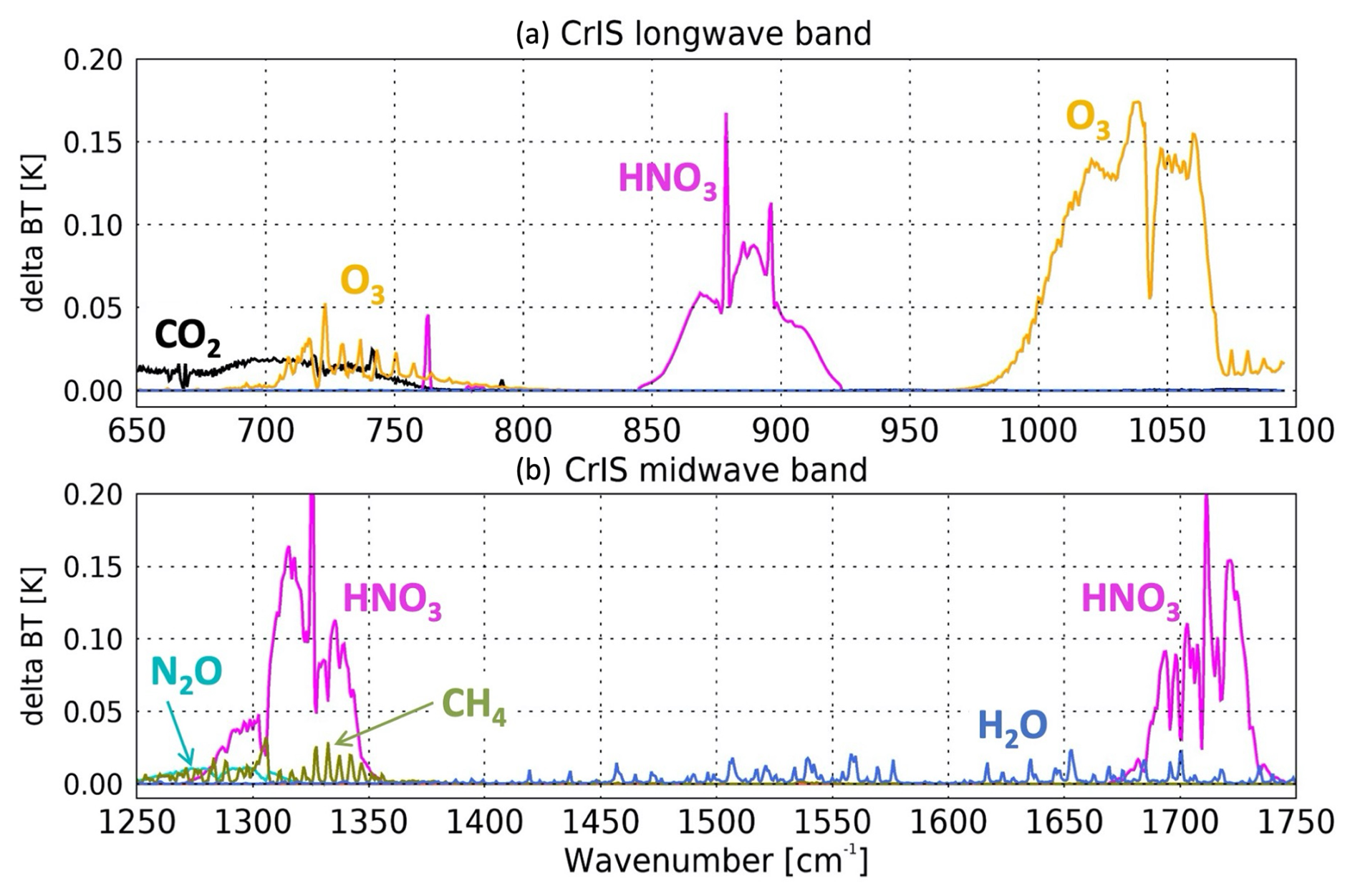
Figure 1 Lower stratospheric (30–90 hPa) trace gas absorption spectra as the absolute delta brightness temperature (BT) for six atmospheric gases active in the thermal IR as measured by CrIS in the (a) longwave (650–1095 cm⁻¹) and (b) midwave (1210–1750 cm⁻¹) bands. These delta-BT spectra were calculated using the SARTA forward model and CLIMCAPS L2 retrievals as state parameters on 3 December 2019 at (76.7° N, 124.1° E). Each gas was perturbed by a fraction in the stated pressure layers as follows: H₂O_vap by 10 %, O₃ by 10 %, HNO₃ by 40 %, CH₄ by 15 %, N₂O by 5 % and CO₂ by 1 %. The CrIS shortwave IR band (2155–2550 cm⁻¹) is absent in this figure because neither O₃ nor HNO₃ are spectrally active in this spectral region.

2 Scientific Rationale

The characterization and monitoring of chemical O₃ loss is one of the primary applications for satellite retrievals of stratospheric HNO₃. In short, HNO₃-containing and ice PSCs initiate the chemical reactions that lead to O₃ loss inside polar vortices (e.g., Solomon, 1999). In addition to playing a key role in the conversion of stratospheric chlorine from benign into reactive O₃-destroying forms, HNO₃ is also involved in the deactivation of chlorine into reservoir forms at the end of winter. Therefore, the degree of chemical O₃ loss within any given polar vortex depends on the temperature and the presence of HNO₃. If PSC particles grow large enough for efficient sedimentation, then HNO₃ can be removed irreversibly from parts of the lower stratosphere (known as denitrification). It is not just the absolute temperature but also the thermal history of an air parcel that affects the state of PSCs and thus the rate of denitrification (Lambert et al., 2016; Murphy and Gary, 1995; Toon et al., 1986). These are complex chemical processes that can be monitored only with an ensemble of observations covering the chemical (e.g., HNO₃ and O₃) and physical (e.g., T_air and PSCs) state of the atmosphere.

Nadir-IR sounders measure HNO₃ with peak sensitivity in the lower stratosphere (30–90 hPa), which is also where PSCs mainly form (e.g., Tritscher et al., 2021). Moreover, AIRS, CrIS and IASI (all in low-Earth orbit) make their measurements in wide swaths (∼ 2000 km) with polar crossings every ∼ 90 min irrespective of sunlight. In other words, not only do nadir-IR sounders observe HNO₃ in the area of interest for O₃ monitoring, but they do so with the ability to generate full-cover maps, both daytime and nighttime. Ronsmans et al. (2018) illustrate this with global maps of FORLI HNO₃ retrievals.

In Fig. 1, we highlight some of the CrIS spectral features to emphasize its sounding capability. CrIS measures the IR spectrum in three distinct bands: longwave IR (650–1095 cm⁻¹), midwave IR (1210–1750 cm⁻¹), and shortwave IR (2155–2550 cm⁻¹). We limit our focus in Fig. 1 to the two CrIS bands that report significant sensitivity to HNO₃, namely the longwave and midwave bands. The absorption features in Fig. 1 were calculated as the absolute difference in brightness temperature (delta-BT) [Kelvin] given a perturbation of the target variable. We used the Stand-alone AIRS Radiative Transfer Algorithm (SARTA; Strow et al., 2003) to calculate these delta-BT spectra with a CLIMCAPS sounding (i.e., the full suite of retrieved variables) as the background atmospheric state. Each target variable was perturbed in the lower stratospheric pressure layers (30–90 hPa), while keeping its value in all other layers constant.

Note the 3 distinct absorption signals for HNO₃ (centred about 890, 1325 and 1725 cm⁻¹) and two for O₃ (centred about 725 and 1025 cm⁻¹). Signals for HNO₃ and O₃ in the longwave band (Fig. 1a) are in the spectral window regions ∼ 850–900 and 1000–1050 cm⁻¹, respectively, which means that these channels have strong sensitivity to the thermodynamic structure of the troposphere, i.e., clouds, surface emissivity and T_air. The HNO₃ signal centred at 1325 cm⁻¹ in the midwave band is, in turn, weakly sensitive to lower stratospheric N₂O and CH₄. We, therefore, regard N₂O and CH₄ as spectral interference (or geophysical noise) in this HNO₃ band. Similarly, the HNO₃ signal centred at 1725 cm⁻¹ has weak sensitivity to stratospheric H₂O_vap. Even though observations of H₂O_vap can be very useful in characterizing chemical processing, the midwave IR band does not have sufficient sensitivity to stratospheric H₂O_vap, relative to all sources of signal and noise, to yield stable retrievals in this part of the atmosphere. Nadir IR sounders are primarily sensitive to tropospheric H₂O_vap, which CLIMCAPS retrieves with high accuracy (Smith and Barnet, 2020, 2023a). As far as O₃ goes, the stratospheric signal centred at 725 cm⁻¹ is not only much weaker than the one centred at 1025 cm⁻¹, but it is also affected by CO₂ and T_air errors. Even though CrIS is a nadir-viewing IR sounder with much lower vertical resolution than MLS, our aim with Fig. 1 is to demonstrate the potential for optimizing CLIMCAPS HNO₃ and O₃ retrievals with respect to the number and spectral range of available IR channels.

3 Retrieval experiments and technical overview of CLIMCAPS

Here we describe the experimental setup for optimizing and characterizing CLIMCAPS HNO₃ retrievals. We give a generalized overview of the CLIMCAPS retrieval approach to clarify how we are able to separate stratospheric and tropospheric HNO₃, while simultaneously minimizing all known sources of geophysical noise in the longwave IR window region (∼ 11 µm). In simplified terms, CLIMCAPS employs the Bayesian inversion equation, as popularized by Rodgers (2000), to iteratively retrieve a set of atmospheric state variables from nadir IR measurements as follows:

$$\begin{array}{}\text{(1)}& \begin{array}{rl}\widehat{x}& =x_{\mathrm{a}}+{\left({\mathbf{K}}^{\mathrm{T}}{\mathbf{S}}_{\mathit{ϵ}}^{-\mathrm{1}}\mathbf{K}+{\mathbf{S}}_{\mathrm{a}}^{-\mathrm{1}}\right)}^{-\mathrm{1}}{\mathbf{K}}^{\mathrm{T}}{\mathbf{S}}_{\mathit{ϵ}}^{-\mathrm{1}}\\ & \times \left[(y-F(x_i\left)\right)+\mathbf{K}(x_i-x_{\mathrm{a}})\right]\end{array}\end{array}$$

where $\widehat{x}$ is the retrieved value of target variable x at iteration i+1, x_a the a priori estimate of x, x_i the retrieved value of x at iteration i, K the Jacobian of the forward model F, S_ϵ the measurement error covariance matrix that quantifies spectral uncertainty, S_a the a priori error covariance matrix, y the instrument measured IR spectrum, and F(x_i) the TOA spectrum calculated by the forward model using a set of background atmospheric state variables.

In Eq. (1), the matrix, S_a, regularizes the degree to which y alters x_a in solving for $\widehat{x}$ such that the smaller the values in S_a, the more $\widehat{x}$ resembles x_a. Stated differently, if x_a approximates the true state of x at the time of measurement (i.e., low uncertainty about x_a, thus small S_a), then the SNR of y will be suppressed (strongly regularized) and x_a will remain largely unaltered in $\widehat{x}$. If, on the other hand, x_a is a generalized estimate (e.g., static climatology) with no bearing on the true state of x at the time of measurement (i.e., high uncertainty about x_a, thus large S_a), then the SNR of y will be weakly regularized and $\widehat{x}$ will have a large departure from x_a. This, however, does not guarantee accuracy in $\widehat{x}$, because the spectral channels sensitive to x measure both signal and noise; if a measurement with small SNR (high noise) is not sufficiently regularized then $\widehat{x}$ could be dominated by errors. But to correctly define S_a for the sake of accuracy in $\widehat{x}$, one needs knowledge of the true state of x at the time of measurement, which is an onerous task given that AIRS, CrIS and IASI measure a wide range of atmospheric conditions across the globe, day and night. In practice S_a is often calculated offline as a generalized, statistical estimate of uncertainty about x_a, which limits the accuracy of $\widehat{x}$.

CLIMCAPS differs from Eq. (1) according to the approach detailed in Susskind et al. (2003) to enable a long-term product with global coverage where $\widehat{x}$ deviates from x_a only when the measurement SNR is quantifiably high to ensure accuracy under a broad range of Earth system conditions. Most importantly, CLIMCAPS does not employ S_a as regularization term but instead regularizes Eq. (1) by diagonalizing the ${\mathbf{K}}^{\mathrm{T}}{\mathbf{S}}_{\mathit{ϵ}}^{-\mathrm{1}}\mathbf{K}$ matrix (or, decomposition onto a set of orthogonal eigenvectors that it then subsets, damps or filters based on the magnitude of the corresponding eigenvalues (λ_j, where 1 < j ≤ number of retrieval layers) and how they relate to a pre-determined static threshold, λ_c (this is discussed in detail in Smith and Barnet, 2020). We derive λ_c empirically for each target variable such that eigenvectors dominated by signal (λ_j > λ_c) are used in the retrieval of $\widehat{x}$, while those dominated by noise (λ_j < λ_c) are filtered out. We should note that CLIMCAPS uses SARTA to calculate finite differencing Jacobians as the K_k,l matrix (where 1 ≤ k ≤ total number of channels and, 1 ≤ l ≤ 100 SARTA pressure layers) that it transforms onto the coarser retrieval pressure grid (on j layers) in solving for $\widehat{x}$. Once retrieved, CLIMCAPS transforms $\widehat{x}$ back onto the 100 SARTA layers for ease of ingest into downstream applications. In each transformation, CLIMCAPS uses S_a in calculating the null space uncertainty as described in Smith and Barnet (2019). The course pressure layers CLIMCAPS uses for each retrieval variable were empirically derived offline as a series of overlapping basis functions to account for the strength and pressure-dependence of the measurement information content (Maddy and Barnet, 2008).

CLIMCAPS defines S_ϵ as an off-diagonal matrix representing uncertainty from all sources of noise affecting (y−F(x_i)), not just y. These include, instrument noise, errors in the measurement and forward model, as well as uncertainty about the atmospheric state needed in the calculation of F(x_i) at each retrieval step, which we refer to as the background atmospheric state, or x_b (Smith and Barnet, 2019). In our case here, where $\widehat{x}$ is HNO₃, x_b includes T_air, H₂O_vap, O₃, CO, CH₄, N₂O, CO₂ as well as Earth surface temperature and emissivity. The instrument noise is random and quantified as the noise equivalent delta temperature (NEdT). The measurement error term includes the systematic, correlated errors introduced by apodization of the radiance measurement (in the case of CrIS, Smith and Barnet, 2025) and as well as the random amplification of NEdT and introduction of systematic errors due to cloud clearing (Smith and Barnet, 2023b). The errors in the forward model, F, is calculated empirically offline to account for all random and systematic sources affecting the accuracy of F(x).

Table 1 details the eight pressure layers CLIMCAPS uses in its HNO₃ retrieval as the hinge points and effective averages. The CLIMCAPS HNO₃ a priori estimate, x_a is a single, static climatological profile that it uses for all retrievals globally. It is also the same profile SARTA employs for its TOA radiance calculations, which is the one developed by the Air Force Geophysical Laboratory (AFGL; Anderson et al., 1986). The AFGL HNO₃ profile represents a global average ranging between 0.01–1.0 ppb in the UTLS, which is orders of magnitude smaller than the stratospheric values retrieved for HNO₃ in the extratropics during wintertime. Future work could focus on re-evaluating this AFGL profile for use as HNO₃ x_a, but the solution is not a simple replacement with a different estimate. As depicted in Eq. (1), $\widehat{x}$ depends on adding measurement SNR to x_a, which means that whenever x_a is high relative to the true state of x, $\widehat{x}$ will be biased high. Given the large dynamic range of HNO₃ during the polar wintertime months, we argue that it is preferable for x_a to be very small so that the retrieved product depict elevated HNO₃ values only where the true state (x_true) is high. Stated differently: when x_true is very small then the corresponding IR measurement SNR for HNO₃ is very low and $\widehat{x}$ will approximate x_a. Conversely, when x_true is large, the measurement SNR is large and $\widehat{x}$ will have a large departure from x_a. This is all the more important for a target variable like stratospheric HNO₃ that is very difficult to represent with an accurate x_a at each space and time retrieval footprint because of the lack of real-time observations. We can have confidence in CLIMCAPS HNO₃ retrievals because $\widehat{x}$ will be low whenever x_true is low, and $\widehat{x}$ will significantly depart from x_a only when the measurement SNR is large.

Table 1 Summary of the 2 CLIMCAPS HNO₃ algorithm components – Bmax and channel selection – tested in this study. Four different Bmax values and 2 different channel selections define 5 experimental setups in total, R1–R5. The righthand column specifies the 9 pressure hinge points and 8 effective mean values of the pressure layers on which CLIMCAPS retrieves HNO₃.

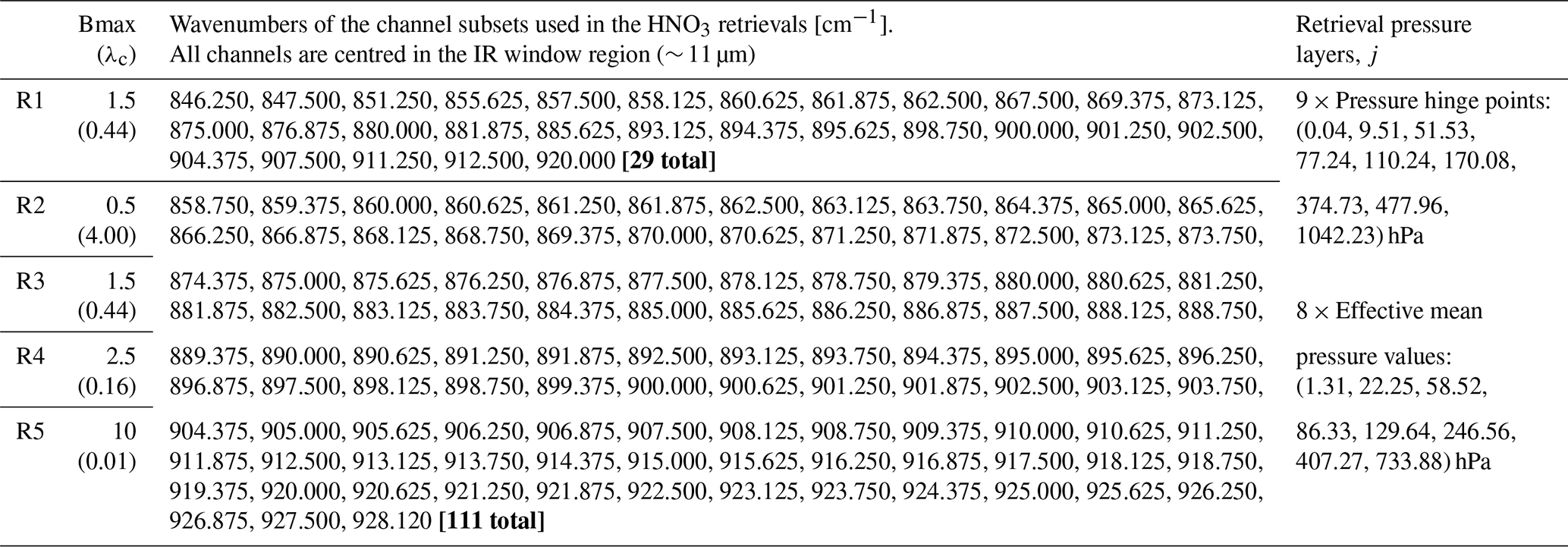
For the sake of demonstrating the feasibility of a nadir-IR stratospheric HNO₃ product in this paper, we focus our experiments on the spectral channel sets and regularization mechanism. Table 1 (column 3) lists the two channel subsets we test, with each subset centred on the 11 µm (∼ 900 cm⁻¹) HNO₃ absorption band (Fig. 1). In addition, the empirical threshold value, λ_c that CLIMCAPS employs for HNO₃ in the regularization of its inverse solution (Eq. 1) is given in Table 1, column 2. CLIMCAPS derives λ_c at run-time using the input scalar variable, Bmax, as follows:

$$\begin{array}{}\text{(2)}& {\mathit{\lambda }}_{\mathrm{c}}=[\mathrm{1}/(\text{Bmax}{)}^{\mathrm{2}}]\end{array}$$

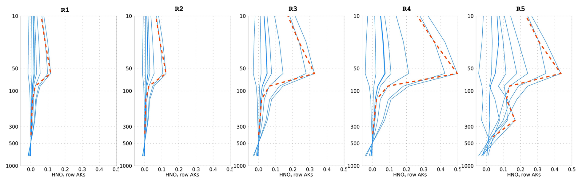
Figure 2 The eight CLIMCAPS averaging kernel (AK) functions (blue lines) for an HNO3 retrieval on 2 February 2020 at 70.9° N, 80.9° E according to each of the five experimental configurations, (left) R1 to (right) R5. CLIMCAPS retrieves HNO₃ on 8 broad pressure layers as defined in Table 1. The dashed red line is the diagonal vector of the 8 × 8 AK matrix to summarize the peak SNR of each AK function.

Both CLIMCAPS and the real-time NUCAPS system have their origins in the heritage AIRS retrieval system (Susskind et al., 2003) and share many algorithm components, as described in Berndt et al. (2023). Historically, HNO₃ was added to the NUCAPS retrieval sequence primarily to improve the T_air SNR (Fig. 1 in Berndt et al., 2023 summarizes this step-wise approach). CLIMCAPS V2.1 takes a similar stepwise retrieval approach, as illustrated in Smith and Barnet (2023a). At every retrieval footprint, CLIMCAPS calculates an averaging kernel (AK) matrix according to Eq. (2) in Smith and Barnet (2020) where each row, or AK, quantifies the SNR of the retrieval system for a target variable about each pressure layer. Stated differently, we can interrogate the AKs to determine the degree to which the SNR at a specific pressure layer is correlated across all other layers. For each HNO₃ retrieval with eight pressure layers, CLIMCAPS, therefore, generates an 8 × 8 AK matrix, or eight AKs across eight pressure layers. Figure 2 depicts the eight AKs of an HNO₃ retrieval on 2 February 2020 at (70.9° N, 80.9° E) for each of the 5 experimental configurations (Table 1). We should note that CLIMCAPS calculates TOA radiance spectra with SARTA, which requires the input state variables to be defined on 100 pressure layers (Strow et al., 2003). These are also the layers on which we report the Level 2 product (Smith and Barnet, 2023a) for ease of ingest into applications downstream. At run-time, however, the profile retrievals are performed on a reduced set of broad pressure levels to more closely represent the information content the measurements have for each target variable (Maddy and Barnet, 2008).

Figure 2 shows that the CLIMCAPS HNO₃ AKs have relatively sharp peaks in the lower stratosphere (∼ 50–90 hPa). By comparison, the FORLI HNO₃ AKs (see Fig. 2 in Ronsmans et al., 2016) are smooth curves with broad peaks (∼ 10–700 hPa) that span the mid-troposphere to stratosphere. The difference in AKs between these two nadir-IR retrieval systems tells us how each system quantifies and harnesses the SNR of the nadir IR measurements with respect to the target variable; FORLI HNO₃ has significant correlation across most of the retrieval layers (which is why they aggregate their product into a single value spanning the stratosphere and troposphere), while CLIMCAPS HNO₃ correlates predominantly across the lower stratospheric layers (which is why we can propose a stand-alone stratospheric product in this paper). Looking more closely at the 5 experimental configurations in Fig. 2, we see that the R1 and R2 configurations have AK values approximating zero in the troposphere (i.e., pressures > 100 hPa) with peaks at ∼ 70 hPa, which is favorable for retrieving lower stratospheric HNO₃ because it means no correlation with tropospheric SNR. However, compared to R3–R5, the R1 and R2 stratospheric SNR is very low overall and thus not ideal. The R5 configuration, in contrast, presents AKs with peaks in both the mid-troposphere and the lower stratosphere, which means that their SNR about HNO₃ is strongly correlated across the troposphere and stratosphere. For a stand-alone stratospheric HNO₃ product, we are interested in a system configuration yielding AKs with distinct, large (relatively speaking) peaks centred about ∼ 70 hPa and approximating zero in the troposphere, which is why R3 and R4 are attractive options for a future CLIMCAPS HNO₃ product. We explain this in more detail later.

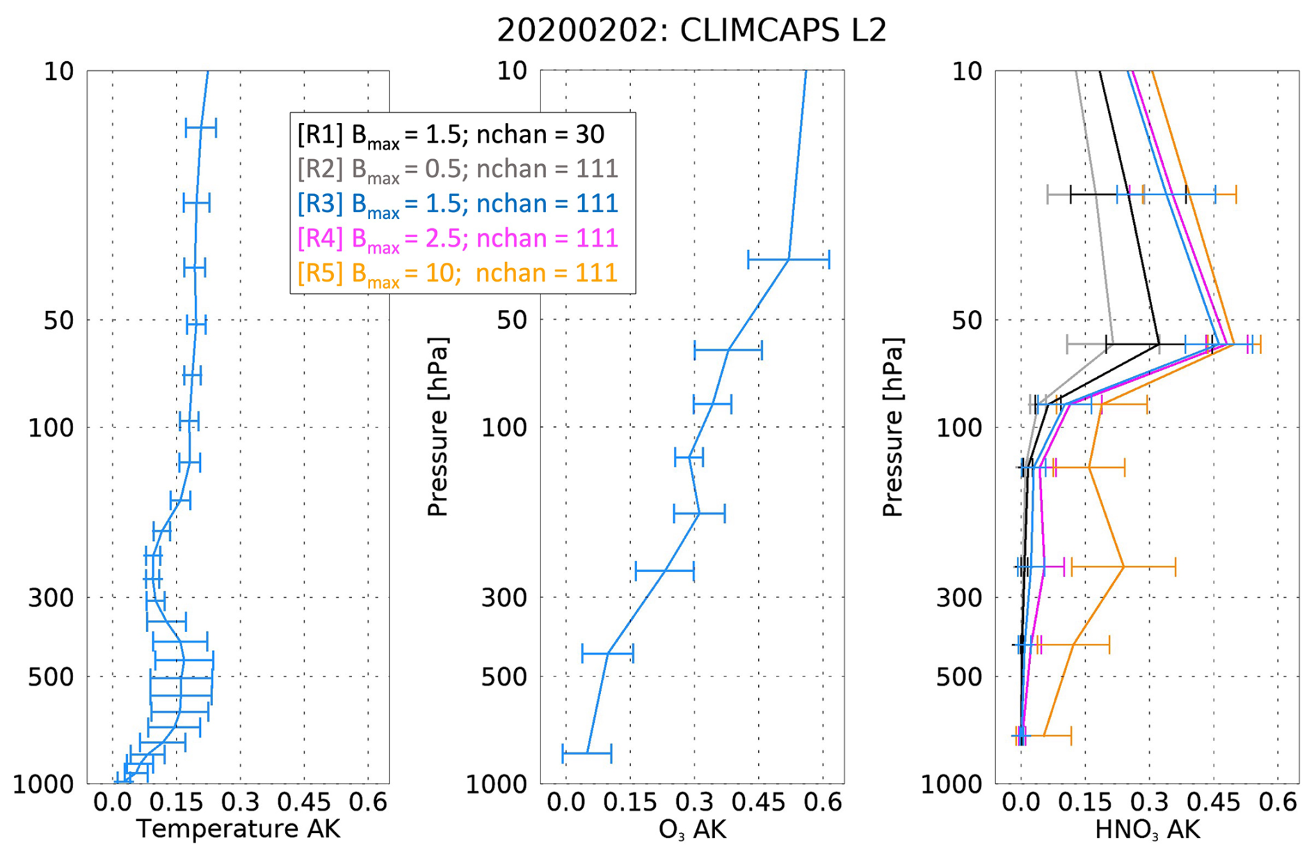
Figure 3 CLIMCAPS averaging kernel diagonal vectors (AKDs) for (left) atmospheric temperature, (middle) O₃ and (right) HNO₃. These pressure-dependent profiles represent the average of all diagonal vectors from the AK matrices reported in the Level 2 product file for each retrieval parameter at every footprint north of 40° latitude on 2 February 2020. The horizontal bars are calculated as the standard deviation of the AKDs to indicate variance with pressure and across the 5 experimental configurations for HNO₃.

In Fig. 2, we also plot the AK matrix diagonal vector (AKD) as a dashed red line for R1–R5. The AKD captures the maximum of each AK and is an effective way to summarize the SNR quantified by the AK matrix. We can then aggregate any number of AKDs statistically as a mean profile with standard deviation error bars (e.g., Fig. 3) for an estimate of system performance within a study region and the degree to which its SNR varies across space and time (Smith and Barnet, 2020, 2025).

An AKD with values significantly greater than zero across two or more pressure layers indicate a system's ability to retrieve the target quantity across those pressure layers. The AKD error bars, on the other hand, can be interpreted as a system's sensitivity to variations in conditions at the time of measurement. However, as discussed in more detail elsewhere (Smith and Barnet, 2025), larger AK peaks and/or variation do not necessarily imply a better system or more accurate retrieval since the exact quantification of measurement SNR under all conditions is very difficult; signal may be misinterpreted as noise and vice versa. The best one can do when designing a Bayesian retrieval system is establish a SNR that yields the desired results with adequate accuracy under most conditions.

As stated earlier, Table 1 lists the two experimental HNO₃ channel sets used here. Experimental run R1 represents the operational CLIMCAPS V2.1 set-up with Bmax = 1.5 and a 30-channel subset selected from the longwave IR window band (850–920 cm⁻¹, or ∼ 11 µm). The only difference between R1 and the operational V2.1 product is that the forward model (or rapid transmittance algorithm) error spectrum (RTAERR) is set to zero in R1. As identified in Smith and Barnet (2025), the V2.1 RTAERR for the CLIMCAPS-CrIS retrieval configuration is too high relative to the CLIMCAPS-AIRS configuration, and we made the recommendation that a future CLIMCAPS V3 release should update the RTAERR accordingly. An overestimated RTAERR lowers retrieval SNR by damping measurement signal, whereas an underestimated RTAERR destabilizes the SNR by allowing forward model noise to be interpreted as signal during retrieval. SNR can be destabilized when the noise is high relative to the signal, or when the noise fluctuates dramatically relative to the signal from scene-to-scene. Additionally, SNR can be destabilized when the noise (random and systematic) is not well-characterized and quantified such that it is wrongly interpreted as signal instead. Similarly, SNR can be destabilized when signal is wrongly interpreted as noise. Here, we simply set RTAERR = 0 for all 5 experimental runs to avoid measurement damping for the sake of illustrating the CLIMCAPS HNO₃ retrieval approach. An operational configuration would require the accurate representation of RTAERR across the full IR spectrum to account for errors introduced by SARTA; however, previous experience suggests that the magnitude of RTAERR is very small and on the order of the instrument noise for most channels. So, while RTAERR = 0 is technically an under estimation, it is close in magnitude to the real RTAERR and therefore not destabilizing. Historically, RTAERR was installed as an attempt to lower the weight of channels that had poor spectroscopic laboratory measurements or a large RTAERR value. In 1995, in the pre-launch AIRS era, this term was expected to be rather large – on the order of ∼ 1 °K for many channels – especially in the water band region. After the AIRS launch, the RTA fitting procedure was improved and more recent laboratory spectroscopy measurements were incorporated so that over time, the RTAERR term was reduced to very low values (< 0.01 °K for most channels). We now simply ignore the few remaining channels that have high RTA errors so that setting RTAERR = 0 is no longer deemed an issue for stability. The HNO₃ channel subset used in R2–R5 employs all available CrIS channels in the ∼ 11 µm band to maximize HNO₃ SNR (111 channels in total). Note that we avoid selecting channels from the two other HNO₃ absorption bands (Fig. 1) because they are spectrally more complex, with multiple sources of interfering signals that manifest as geophysical noise in the retrieval. The IR window region, on the other hand, provides a strong SNR for stratospheric HNO₃ because the predominant source of geophysical noise is from the troposphere, which CLIMCAPS separates out ahead of the inversion step.

We varied Bmax in the R2, R4 and R5 experimental runs from low to high: 0.5, 2.5 and 10.0, respectively (Table 1). Eigenvalues are a dimensionless quantity that represents the HNO₃ SNR. CLIMCAPS uses λ_c in its regularization of the Bayesian inverse solution at run-time (Eq. 1). A measurement eigenfunction is used without any damping (i.e., determined 100 % in the retrieval) when its eigenvalue (λ_j) exceeds λ_c. In contrast, the eigenfunctions for which λ_j < λ_c are either regularized (damped) or removed from the solution space altogether (filtered). The regularization factor, Rfac_i, determines how the eigenfunctions are treated as follows:

$$\begin{array}{}\text{(3)}& {\text{Rfac}}_j={\displaystyle \frac{{\mathit{\lambda }}_j}{({\mathit{\lambda }}_j+\mathrm{\Delta }\mathit{\lambda })}},\text{ where }\mathrm{\Delta }\mathit{\lambda }=\sqrt{{\mathit{\lambda }}_{\mathrm{c}}}\sqrt{{\mathit{\lambda }}_j}-{\mathit{\lambda }}_j\end{array}$$

When 0.05 < Rfac_j < 1.0, the corresponding eigenfunction is damped anywhere between 0.01 % to 95 % as determined by the relation 100.0(1−Rfac_j). All eigenfunctions for which Rfac_j ≤ 0.05 are simply removed (or damped 100 %) because the assumption is that these high-frequency eigenfunctions are dominated by noise relative to the target variable. In summary, a high Bmax corresponds to a low λ_c, which means that Rfac_j will be higher overall with a larger set of eigenfunctions satisfying the conditions λ_j > λ_c. If Bmax is too low for a target variable, then the measurement signal may be overdamped such that the top eigenfunctions all have λ_j≪λ_c. Conversely, if Bmax is too high, then measurement noise may be underdamped, with higher-order eigenfunctions – that contain mostly noise relative to the target variable – contributing to the solution. In such cases, the retrieval SNR is destabilized, which can result in retrievals that do not converge or AKs that are misshapen. We consider Bmax to be optimized for a target variable when it enables CLIMCAPS regularization to effectively function as a noise filter during run-time. It is worth emphasizing that these eigenfunctions represent the orthogonal vectors of the measurement SNR matrix, ${\mathbf{K}}^{\mathrm{T}}{\mathbf{S}}_{\mathit{ϵ}}^{-\mathrm{1}}\mathbf{K}$, where S_ϵ represents all errors in (y−F(x)) as discussed earlier.

Table 2 illustrates how Bmax works in practice for seven profile retrievals – T_air, H₂O_vap, CO₂, O₃, CH₄, CO and HNO₃ – given the R4 CLIMCAPS configuration. Tabulated like this, it becomes clear how the measurement signal for T_air, H₂O_vap, CO₂, O₃ and CH₄ is spread across multiple eigenfunctions and, in contrast, concentrated into a single dominant eigenfunction for CO and HNO₃. All eigenfunctions with Rfac values less than 5 % are removed (filtered) from the solution space and thus treated as containing only noise relative to the a priori estimate. The measurement SNR matrix, ${\mathbf{K}}^{\mathrm{T}}{\mathbf{S}}_{\mathit{ϵ}}^{-\mathrm{1}}\mathbf{K}$, projected onto an orthogonal vector space like this captures the signal by the first few eigenfunctions, while the noise separates out into the remaining eigenfunctions. Looking more closely at H₂O_vap, we see that EF1 is fully determined in the retrieval (no damping), while EF2 is damped 55 %, EF3 82 %, EF4 87 % and EF5 93 %. It is different for T_air, for which EF1 through EF8 are all damped to some degree, with EF1 9 % and EF8 95 % as the extremes. When we look at O₃, we see by far the highest EF1 eigenvalue of all the variables listed. This can be explained by the fact that nadir-IR sounders have very strong sensitivity to stratospheric O₃ in the 1000–1100 cm⁻¹ band (Fig. 1) and almost negligible sensitivity to other background state variables in this spectral region. In addition to a high SNR for EF1, the O₃ EF2 and EF3 have eigenvalues that are relatively high as far as nadir-IR trace gas signals go, indicating the presence of a tropospheric O₃ signal. As demonstrated in Smith and Barnet (2020, 2025), the nadir-IR sounder sensitivity to tropospheric O₃ is high enough to warrant a profile product, which Gaudel et al. (2024) evaluated as part of the Tropospheric Ozone Assessment Report 2 (TOAR-II).

Table 2 Eigenvalues and DOFS from an R4 run for seven retrieval variables – T_air, H₂O_vap, CO₂, CO, CH₄, O₃ and HNO₃ – at a single retrieval footprint. Row 1 reports the static Bmax threshold (and corresponding λ_c value) that CLIMCAPS employs at run-time to determine the degree of regularization for the Bayesian inverse solution. Row 2 details the eigenvalues (λ_j) and corresponding regularization factor, Rfac_j,of the top eight eigenfunctions (EF1–EF8). No eigenvalues with Rfac_j < 5 % are considered in the retrieval (or damped 100 %). The bottom row reports the DOFS calculated as the sum total of all Rfac_j values.

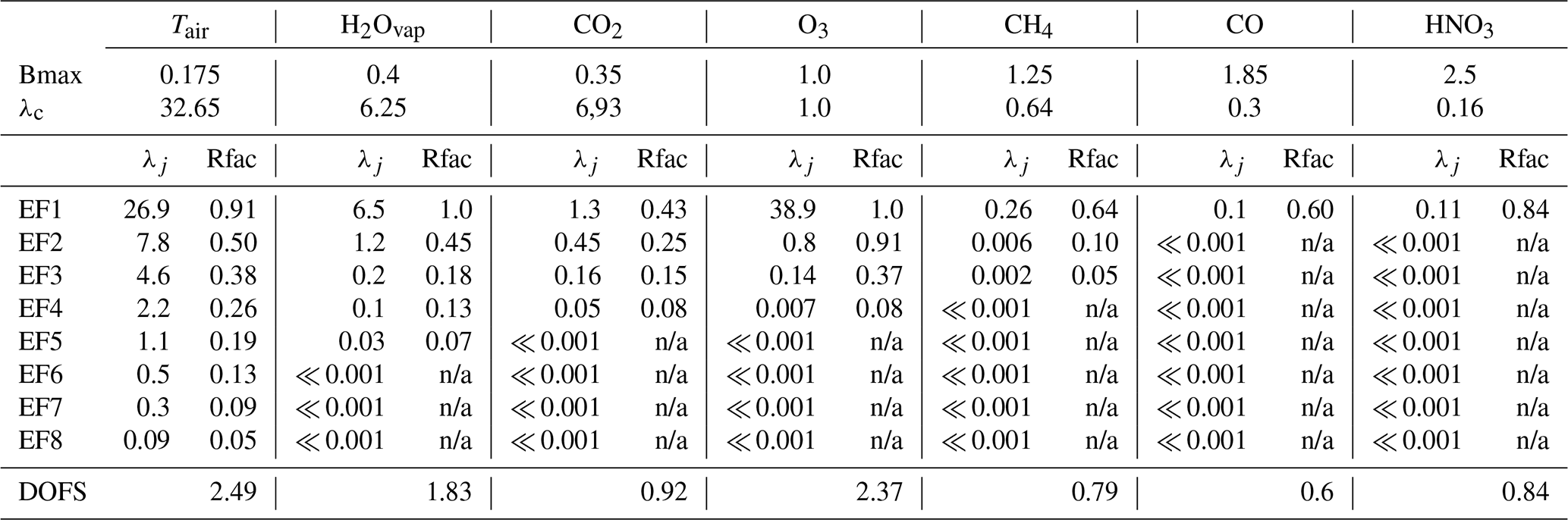
n/a: not applicable.

There is a direct relation between CLIMCAPS regularization and the retrieval AKs. A system that is over-regularized (i.e., where signal is quantified as noise) will have AK peaks approaching zero, and a system that is under-regularized (i.e., where noise is quantified as signal) will have AK peaks approaching one. All measurements have some degree of noise, so AK peaks typically range between zero and one (Smith and Barnet, 2020). CLIMCAPS has a comprehensive error (and uncertainty) quantification scheme that accounts for the manner in which prevailing atmospheric and Earth surface conditions affect measurement SNR. This means that CLIMCAPS AKs can be used as a diagnostic metric in the analysis of system performance and the interpretation of product differences in inter-comparison studies. Another useful metric is the degrees of freedom for signal (DOFS) that is calculated as the trace of the AK matrix (or sum total of the AKD) to indicate the number of independent pieces of information that can be retrieved about the target variable, given the measurement SNR at a specific space and time location. DOFS = 1 means a single distinct quantity, DOFS = 2 means two distinct quantities, and so on. However, nadir-IR retrieval DOFS are rarely whole numbers, and the signal available for a target variable about a pressure layer is never noise-free, so in practice DOFS is a fractional value. Table 2 summarizes the CLIMCAPS DOFS for seven retrieval variables given the R4 configuration on 2 February 2020. Note how the DOFS for T_air, O₃ and H₂O_vap all exceed one, indicating measurement SNR for multiple atmospheric layers. In contrast, the DOFS for CO₂, CH₄, CO and HNO₃ are all below one. Upon closer inspection, we can see that the SNR (given by the eigenvalues, λ_j) for CO₂ and CH₄ are spread across multiple eigenfunctions, while CO and HNO₃ depend on the SNR from a single eigenfunction. This indicates that the information for CO₂ and CH₄ is not only low but also spread across multiple pressure layers, which is why we recommend integrating the retrievals into total column values ahead of their use in applications (Frost et al., 2018; McKeen et al., 2016; Smith et al., 2021). The SNR for CO and HNO₃, in contrast, is concentrated into a single eigenfunction, which indicates that the retrieved quantity is concentrated in a single pressure layer; as seen in the HNO₃ AKs (Fig. 2), it is centred in the lower stratosphere.

Another mechanism CLIMCAPS employs to maximize the SNR for each target variable is channel selection. We calculate the statistical probability of each IR channel to observe the target variable offline using the method described in Gambacorta and Barnet (2013). This means that the channel subsets are static across all retrieval footprints for a given product version (see Smith and Barnet, 2025 Supplement for a list of all the CLIMCAPS V2.1 channel sets). However, future system upgrades and reprocessing of the multi-decadal record can readily employ different channel subsets, so there is no requirement for the channel subsets to be fixed for all future versions of CLIMCAPS. In contrast, the degree to which the signal is captured (and noise is filtered) from the orthogonal measurement subset (eigenfunctions) is determined dynamically for each retrieval footprint at run-time. Given the changing climate, we consider this an important capability, especially for a multi-decadal product like CLIMCAPS, which cannot risk biasing its observational time-series with static assumptions about a priori uncertainty and its covariance, $\mathit{\delta }{x}_{{\mathrm{HNO}}_{\mathrm{3}}}\mathit{\delta }{x}_{{\mathrm{HNO}}_{\mathrm{3}}^{\mathrm{T}}}$, as the regularization term. The goal of the CLIMCAPS HNO₃ product we propose here is to observe polar climate processes, not reflect static assumptions.

CLIMCAPS retrieves cloud top pressure and cloud fraction, but only for the troposphere, so it does not have the ability to report on PSCs that initiate heterogeneous chemical processing in the polar stratosphere. Another factor to keep in mind is that CLIMCAPS performs “cloud clearing” on each cluster of 3 × 3 instrument fields-of-view (FOVs; ∼ 15 km at nadir) and retrieves all geophysical variables on the aggregated footprint (∼ 50 km at nadir). Cloud clearing uses spatial information to remove the spectral cloud signal from each measurement before inversion (Smith and Barnet 2023b), and it allows CLIMCAPS to quantify (and propagate) measurement error due to clouds in all atmospheric state retrievals. This not only helps stabilize the SNR, but also affords the ability to derive meaningful quality control (QC) metrics. One of the criteria in the CLIMCAPS QC flag is to reject retrievals with high error due to cloud contamination. All CLIMCAPS retrievals, therefore, represent the atmosphere around cloud fields, not inside them.

We ran CLIMCAPS on the JPSS-1 Level 1B files of CrIS and ATMS (Advanced Technology Microwave Sounder). We refer to the experimental configuration employed in this paper simply as CLIMCAPS to indicate that the results apply to all sounder configurations in general and to distinguish it from the operational implementation of CLIMCAPS V2.1 at the GES DISC. The Level 2 retrieval files report values on the nadir-IR sounder instrument grid. There are 45 scanlines per file, and each scanline spans nearly 2000 km with 30 retrieval footprints along track, such that the spatial resolution at nadir is ∼ 50 km and at edge-of-scan ∼ 150 km. These satellites orbit the Earth from pole to pole, so their wide swaths have significant overlap at high latitudes. A number of custom configurations for creating gridded Level 3 files are possible, depending on the target application. For the sake of illustration and clarity of argument, we aggregated the CLIMCAPS retrievals from all ascending JPSS-1 orbits (∼ 13:30 local equator overpass time) onto 4° equal-angle global grids. Before aggregation, we vertically integrated the T_air, O₃ and HNO₃ profiles over all pressure layers in the 30–90 hPa range. Only those retrievals that passed CLIMCAPS QC were aggregated. We added DOFS to the suite of gridded variables to help interpret the results. CLIMCAPS QC is a simple “yes/no” flag derived from a large array of diagnostic metrics that includes errors due to cloud clearing, T_air, H₂O_vap, and cloud fraction. As our understanding of product applications matures, we envisage future CLIMCAPS upgrades to include customized QC metrics, especially for the trace gas species.

Table 3 A summary of the top 5 HNO₃ eigenvalues for 2 distinct retrieval footprints as processed by each experimental configuration, R1–R5. The eigenfunctions of the radiance measurements are dependent on channel selection but independent of λ^′ (Eq. 2), which is an empirical scalar that determines the CLIMCAPS Bayesian regularization factor, Rfac_j (Eq. 3). The DOFS for each configuration and footprint is listed to indicate the correlation between information content and the degree to which the eigenfunctions are regularized (i.e., sum of all Rfac values).

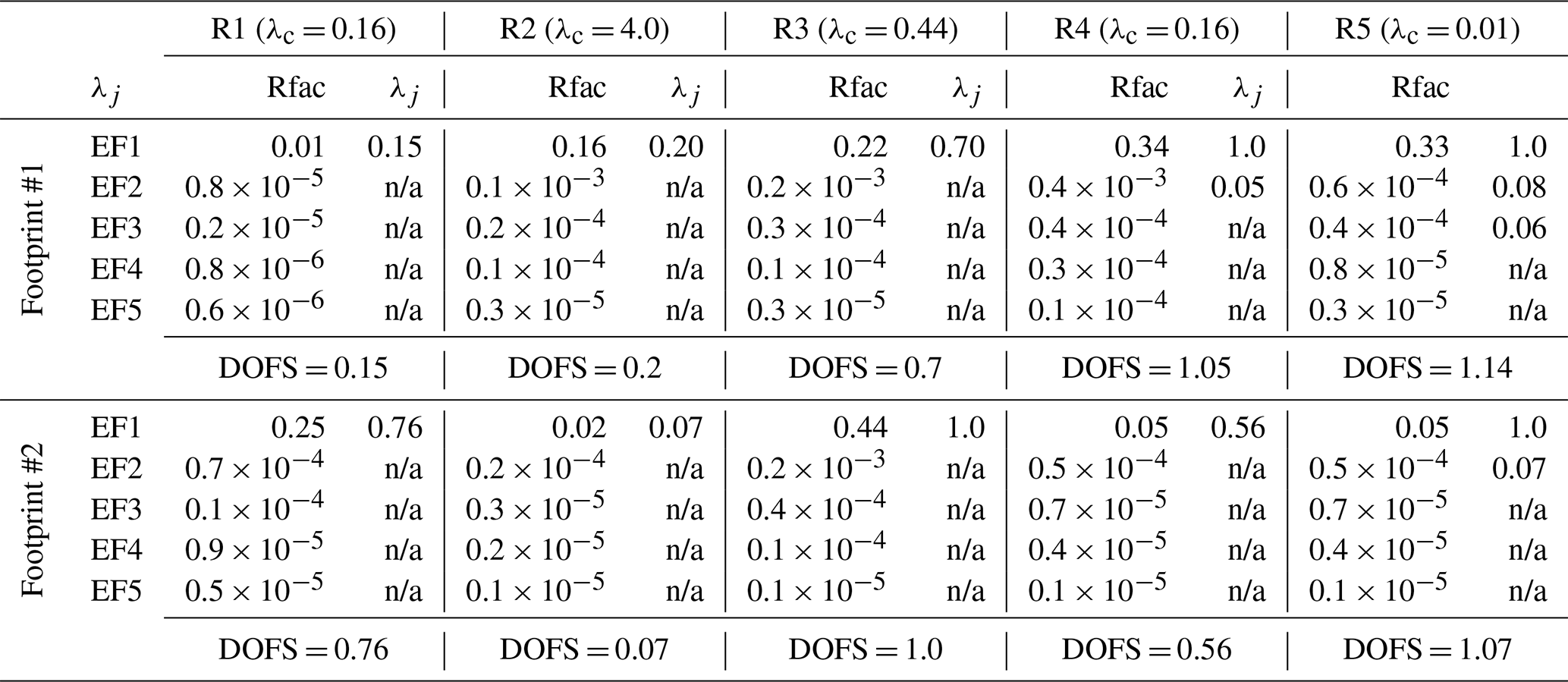
n/a: not applicable.

4 Results and Discussion

Having described the dynamic regularization mechanism of the CLIMCAPS inversion in Sect. 3, we now turn our attention to evaluating the five experimental runs, R1–R5. Figure 3 depicts the AKDs (mean profile and standard deviation error bars) for all CLIMCAPS retrievals of T_air, O₃ and HNO₃ poleward of 40° N latitude on 2 February 2020. The first point to note is that the T_air and O₃ AKD profiles have error bars for more pressure layers than the HNO₃ AKD. This is because nadir-IR sounders generally have higher information content for T_air and O₃ relative to that for HNO₃. CLIMCAPS, accordingly, has a unique set of basis functions for each profile variable to allow the measurements to reliably map into retrieval space given the available information content. The higher the DOFS on average, the more retrieval layers are warranted. These retrieval layers are static across all retrieval footprints.

There are 5 HNO₃ AKDs in Fig. 3, corresponding to the 5 experimental runs. As mentioned, R1 is closest to the CLIMCAPS V2.1 configuration, except that RTAERR = 0. The HNO₃ AKs for all 5 runs have peak sensitivity in the lower stratosphere, 30–90 hPa. We selected all available CrIS channels in the longwave IR window region (850–920 cm⁻¹) for the R2–R5 CLIMCAPS runs to maximize measurement SNR for the sake of illustration. This is the same spectral region exploited for HNO₃ retrievals from GLORIA (Oelhaf et al., 2019) and IASI (Ronsmans et al., 2016). With everything else held constant, the only parameter that varies among R2 (grey), R3 (blue), R4 (magenta) and R5 (gold) is Bmax. It is, therefore, all the more remarkable to see how the corresponding HNO₃ AKDs vary, not only in vertical structure, but also in their deviation about the mean in each effective pressure layer. R2 registers the lowest values for HNO₃ AKs overall, and R5 the highest. R3 and R4 result in AKs with similar vertical structure and variance, with R4 having slightly higher AKD values in the middle to upper troposphere.

In general, we know that IR sounder information content varies with ambient conditions, especially in the troposphere, where atmospheric variables have a large dynamic range in response to Earth surface and weather events (Smith and Barnet, 2019, 2020). So, we expect CLIMCAPS AKs to reflect this dynamic range with standard deviation error bars > 0.0. In general, Bayesian AKs with larger (smaller) peaks indicate an inverse solution with stronger (weaker) dependence on the measurement relative to the a priori estimate. In principle, AK = 0 indicates that the solution is the a priori estimate, and AK = 1.0 indicates that the solution is entirely measurement-based with no dependence on an a priori estimate. But measurements contain both signal and noise, so neither of these extremes manifest in reality. While a strong contribution from the measurement (sharply peaked AK) could be interpreted as preferable (e.g., to compensate for a priori uncertainty), one should always keep in mind that measurements contribute noise along with signal. So, a large AK value may very well indicate that the retrieval is dominated by measurement noise, not signal. This is why dynamic regularization of the inverse problem at run-time has proven to be such a robust mechanism for CLIMCAPS retrievals since the eigenvalue decomposition of each measurement SNR matrix helps filter noise. This simplifies error quantification during retrieval and minimizes the probability that retrievals are contaminated by measurement noise that is difficult to identify and quantify otherwise. Note that by “measurement noise”, we do not simply mean the instrument error spectrum (or noise equivalent delta temperature, NEdT). Rather, measurement noise encapsulates all spectral information not directly related to a target variable. For example, the CrIS channels sensitive to mid-tropospheric CH₄ are also sensitive to mid-tropospheric H₂O_vap (Smith and Barnet, 2023a). If the target variable is CH₄, then H₂O_vap should be treated as geophysical noise, and vice versa. Smith and Barnet (2019) explain how we account for the many sources of measurement noise in CLIMCAPS.

Table 3 tabulates the eigenvalues and regularization factor (Rfac_j) relative to HNO₃ for the first 5 eigenfunctions (EF1–EF5) of each experimental run. We report these values for two retrieval footprints independent of each other as well as the footprint represented in Table 2. Bmax determines the eigenvalue threshold, λ_c. In turn, Rfac_j depends on the corresponding eigenvalue, λ_j as well as λ_c. Table 3 illustrates the degree to which the HNO₃ eigenfunctions are regularized in the inverse solution at run-time. The EF2 eigenvalue is orders of magnitude smaller than the one for EF1, and all remaining eigenvalues (EF3–EF5) are roughly the same order of magnitude as EF2. As shown in Table 2, this is not the case for all CLIMCAPS retrieval variables. What it tells us is that most (if not all) of the signal for stratospheric HNO₃ compresses into a single eigenfunction that can readily be isolated from most (if not all) tropospheric signal and noise. With this table and associated discussion, we aim to illustrate how CLIMCAPS regularization works in practice and the things we consider when planning a system upgrade. The results presented in this paper help us identify which experimental configuration to adopt, test and refine for a future V3 public release. An in-depth quantification of the eigenfunctions across all retrieval footprints, and especially the type of conditions of interest to seasonal monitoring in the extratropics, will be the focus of future work. Our objective here is simply to draw broad conclusions about each experimental configuration for the sake of identifying the path forward.

Comparison of the eigenvalues in Table 3 to the AKD profiles in Fig. 3 illuminates the observed differences. At the extremes are R2 (Bmax = 0.5) and R5 (Bmax = 10.0). The former harvests signal exclusively from the first eigenfunction in both cases, while the latter does so from 2 or more. This difference manifests in the R2 AKDs (grey) approaching zero in the troposphere, while the R5 tropospheric AKDs (gold) not only exceed 0.0 by a significant margin, but they also display a large dynamic range. Additionally, of all 5 runs, the R2 AKDs register the lowest values in the stratosphere overall. We attribute this to overdamping. With Bmax set to 0.5, R2 has the highest threshold for determining whether an eigenfunction should be damped in the retrieval, with λ_c = 4.0. We have yet to observe a CLIMCAPS HNO₃ eigenvalue exceeding 4.0. This means that the first HNO₃ eigenfunction will always be damped in R2, irrespective of signal strength. Not only does λ_c determine which eigenfunctions to damp, it also determines the degree to which they are damped, such that the larger the difference between λ_c and λ_j, the smaller the Rfac_j values, and the higher the degree of damping. R2 illustrates how CLIMCAPS has the ability to overdamp nadir-IR measurements to the detriment of the inverse solution. Given that our objective with CLIMCAPS is to harvest as much of the available measurement signal as possible, while simultaneously accounting for most of the known sources of measurement noise, the value assigned to Bmax is an important consideration.

There is more to diagnose from the results presented in Table 3. R5 has the highest Bmax (lowest λ_c) of all the runs, yet in the stratosphere its AKDs approximate those from R3 and R4 (Fig. 3). Moreover, irrespective of retrieval configuration, the HNO₃ AKDs are always much smaller than 1.0, even at their peak around 50 hPa. We deduce that there must be an upper limit to the measurement signal for HNO₃, regardless of system parameters. In Table 3, we see that the eigenvalues of EF1 are always much less than 1.0, unlike those for T_air, H₂O_vap, O₃ and CO₂ (Table 2). This is because nadir-IR sensitivity to stratospheric HNO₃ is low even if the system is optimized.

When DOFS = 1.0, it means that the measurements contain one piece of information about the target variable. But this does not imply that one piece of measurement signal perfectly maps into one piece of atmospheric retrieval during inversion. For CLIMCAPS products, it simply means that the equivalent of one eigenvector determined the inverse solution in all pressure layers at a specific retrieval footprint. One can expand this argument as follows: the R1–R3 configurations rarely have DOFS exceeding one. As seen in Fig. 3, these are also the AKDs with tropospheric values approaching zero. Only R4 and R5 have tropospheric AKDs visibly greater than zero, and they are also the only two configurations often yielding DOFS > 1.0. This leads us to conclude that EF1 contains most of the available stratospheric signal for HNO₃, while EF2 and EF3 almost exclusively quantify tropospheric signal and noise. This clear distinction between EF1 and the other eigenfunctions is not the case for all retrieval variables. Table 2 illustrates that T_air, for example, depends on multiple eigenfunctions, all partially damped but none completely undamped. Wespes et al. (2007) reported that the DOFS of retrievals from IMG radiances range between 0.7 and 1.8 and concluded that this implied the ability of IMG measurements to provide two independent pieces of HNO₃ information – tropospheric and stratospheric partial columns. While a similar range is recorded for IASI HNO₃ DOFS (Ronsmans et al., 2016; Wespes et al., 2022), the retrievals are nonetheless presented as total column values. When a HNO₃ retrieval system, like FORLI, regularizes its Bayesian inversion along the full atmospheric column, without the ability to filter measurement noise at run-time, the stratospheric and tropospheric retrievals are correlated because their spectral SNR is correlated. A total column is, therefore, the only way to report such a retrieval to obtain a stable product. We argue that the CLIMCAPS approach to Bayesian inversion, on the other hand, benefits HNO₃ specifically because the stratospheric and tropospheric SNR can be decomposed into two separate eigenfunctions. This, of course, does not mean that it is the only Bayesian approach with the ability to distinguish an independent piece of stratospheric HNO₃ information. Compared to FORLI, however, CLIMCAPS has this novel capability.

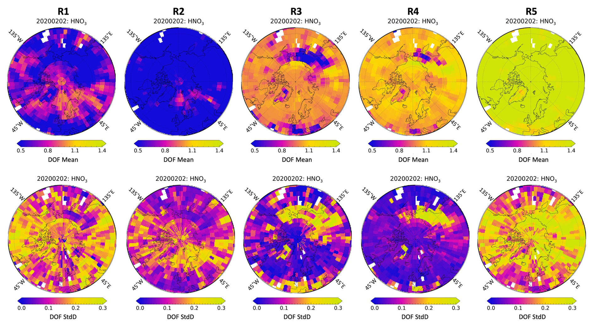
Figure 4 CLIMCAPS information content metrics, as the degrees of freedom for signal (DOFS), aggregated onto a 4° equal-angle grid poleward of 40° N latitude. (Top row) Average of the HNO₃ DOFS. (Bottom row) Standard deviation (SD) of the HNO₃ DOFS. (Left to right) The 5 experimental configurations as defined in Table 1.

Another aspect worth noting is that both R1 and R3 have Bmax = 1.5 (λ_c = 0.44), yet stratospheric R1 AKDs (Fig. 3, black) are significantly smaller than those from R3 (blue). This is due to the fact that the R1 eigenfunctions are derived from 30 nadir-IR channels and those for R3 from 111 channels. It is tempting, therefore, to conclude that this supports the use of all available channels during retrieval, but that would be an over-simplification. Figure 1 (as well as Fig. 2 in Smith and Barnet, 2020) illustrates how nadir-IR measurements are highly mixed signals of multiple Earth system variables. We also know, empirically, that measurement SNR with respect to a target variable varies substantially because it depends on ambient conditions. One can enhance the effectiveness of CLIMCAPS regularization during inversion by pre-selecting measurement subsets with a high probability of SNR > 1.0. This means selecting channels with high sensitivity and low geophysical noise (interference from background state variables) with respect to the target variable.

Figure 4 summarizes our discussion of DOFS for R1 through R5 with maps of the NH centred on the North Pole on 2 February 2020. The gridded average of DOFS, which we refer to as avg(DOFS) from here on, is displayed in the top row, with the standard deviation of the gridded DOFS, or SD(DOFS), on the bottom. R1 and R3 yield similar spatial patterns for avg(DOFS) but different patterns for SD(DOFS). With the R1 eigenfunctions derived from 30 channels, unlike 111 in R3, it is possible that the smaller channel set lowers R1 SNR to the point that its retrieval DOFS become unstable (i.e., highly variable). Given what we have learned from the values reported in Table 3, we argue that it is preferable for HNO₃ DOFS to approximate 1.0 – never to exceed it – and for EF1 to be fractionally damped only for the cases where the measurement SNR is low to begin with, such as where stratospheric HNO₃ concentrations are low. It is, therefore, interesting to compare R3 and R4. Their SD(DOFS) patterns are similar in that SD(DOFS) is high wherever avg(DOFS) is low, despite the R3 avg(DOFS) being much lower overall and R4 avg(DOFS) approximating 1.0 across most of the study area. We can make sense of this when we revisit Tables 2 and 3, which show that Rfac_j can have a large dynamic range – and thus high SD(DOFS) – for small variations in all λ_j < λ_c. So even though R3 may yield a relatively stable HNO₃ retrieval given its low SD(DOFS) across most of the study region, its avg(DOFS) indicate that EF1, or the eigenfunction with most of the stratospheric HNO₃ signal, is probably overdamped. Of all 5 cases, we argue that R4 yields the closest representation of what is needed for a stratospheric HNO₃ product aimed at science objectives related to ozone chemistry. In contrast, R2 and R5 epitomize what is not desirable in a stratospheric HNO₃ product, but for different reasons.

The maps in Fig. 4 indicate that R2 SD(DOFS) is low wherever R3 SD(DOFS) is high (and vice versa), even though their avg(DOFS) maps show not dissimilar patterns. As discussed earlier, the R2 configuration is associated with a very high λ_c, relatively speaking. And, the higher the λ_c, the larger the difference between λ_EF1 and λ_c, leading, in turn, to a lower Rfac_j and lower retrieval DOFS overall. In fact, the R2 difference between λ_c and λ_EF1 is so large that EF1 is always strongly damped, i.e., Rfac_j is small and DOFS low. This is why the R2 avg(DOFS) is overall significantly lower than that of all other configurations in Fig. 4.

In contrast, R5 avg(DOFS) exceeds 1.0 across the whole study area. This is not ideal because it means that the stratospheric HNO₃ retrieval is correlated with tropospheric noise. Two regions of the R5 SD(DOFS) map stand out as having values significantly higher than the background, namely the zones centred about (i) (40–90° N, 50–120° E), or the Siberian landmass, and (ii) (40–60° N, 40–160° W), which is North America. The Earth surface, boundary layer conditions and tropospheric weather processes are highly variable over land. When HNO₃ DOFS > 1.0, the measurement SNR for tropospheric conditions contributes to the retrieval as higher-order eigenfunctions that are damped anywhere between 0.01 % to 95 % according to Rfac_i. This leads us to conclude that it may be worth considering a customized HNO₃ configuration for future CLIMCAPS upgrades. For example, the Rfac of EF2 (and all higher-order eigenfunctions) can be set to a static value (≤ 0.05) to always filter higher-order eigenfunctions, except EF1, to cap DOFS at 1.0 and thus isolate the stratospheric HNO₃ SNR. Of course, more research would need to be done to determine if such an approach is feasible under all conditions (i.e., demonstrate EF2 is always tropospheric), but CLIMCAPS could support such a customization in principle.

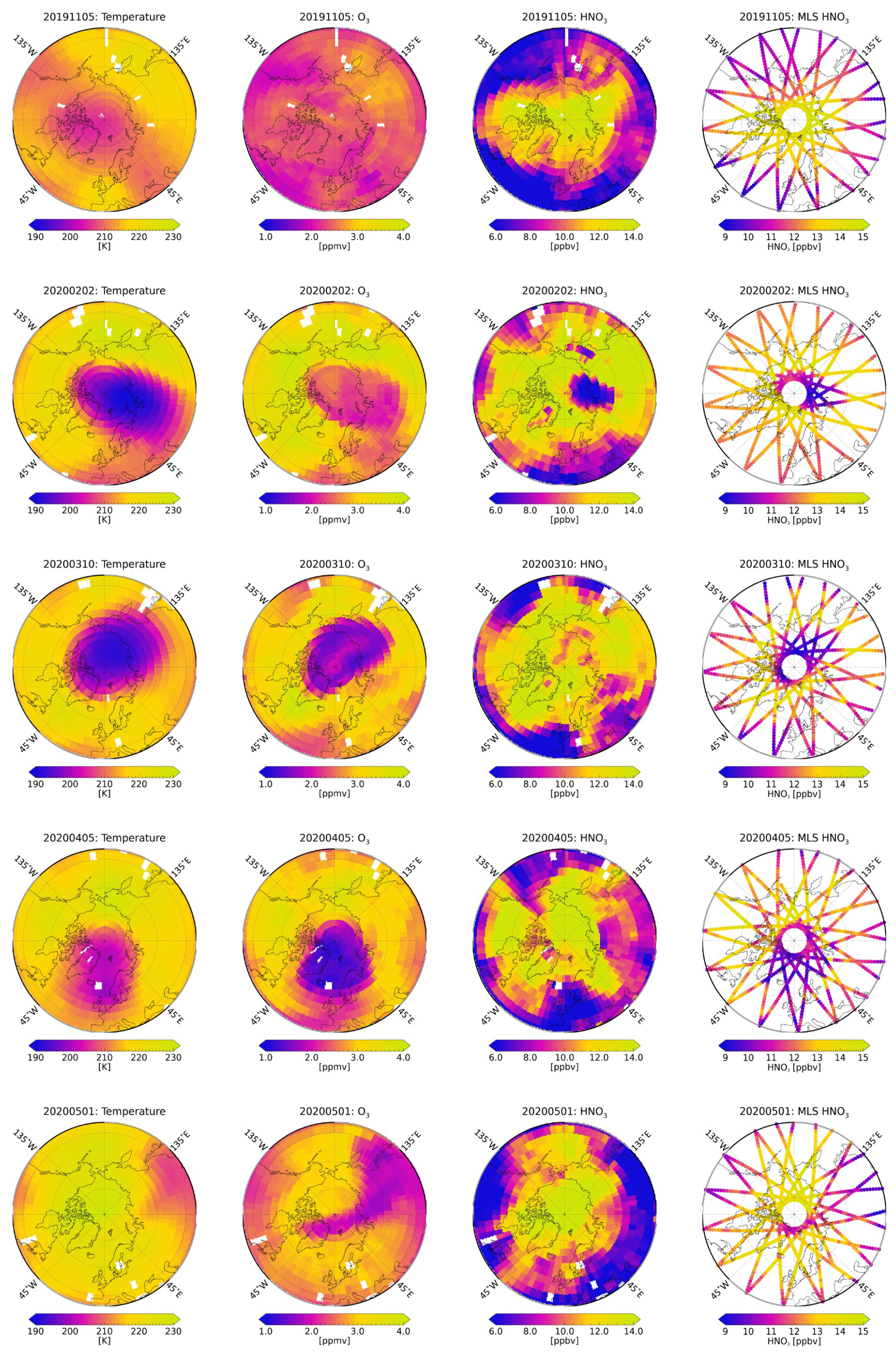
Figure 5 A time series of lower stratospheric CLIMCAPS retrievals of Tair, O₃, and HNO₃ produced by the R4 experimental configuration aggregated onto a 4° equal-angle grid throughout the 2019/2020 Northern Hemisphere winter 635 season poleward of 40° N latitude. The column on the right represents the MLS V5 Level 2 profile HNO3 retrievals at 1.5° intervals. Both the CLIMCAPS and the MLS profile products were vertically integrated across their respective retrieval layers spanning 30–100 hPa.

We contrast the CLIMCAPS HNO₃ retrievals from the R4 experimental configuration with those from limb-viewing MLS in Fig. 5 for 5 d spanning the Northern Hemisphere winter of 2019/2020. CLIMCAPS HNO₃ has global coverage (90° S to 90° N) and is presented here as spatial averages on a 4° equal-angle grid. The MLS product is the Level 2 V005 HNO₃ mixing ratio (Manney, 2021) that has near-global coverage (82° S to 82° N) and profile retrievals spaced 1.5° along the orbital track with roughly 15 orbits per day. We integrated both profile products across their retrieval layers spanning 30–100 hPa for ease of comparison. This figure depicts the formation and dissipation of the Arctic vortex as illustrated by the coincident CLIMCAPS retrievals of stratospheric T_air and O₃. We present CLIMCAPS V3 improvements for T_air and O₃ in a different paper and focus our discussion here on the comparison between MLS and CLIMCAPS retrievals of HNO₃. It is clear that MLS observes a much stronger HNO₃ spatial feature inside the Arctic vortex throughout the winter season. Note how the spatial patterns of CLIMCAPS HNO₃ strongly align with those from MLS at the onset of the vortex in November, and again as HNO₃ reaches its first distinct seasonal feature in February. By March, however, the CLIMCAPS HNO₃ feature weakens relative to that from MLS and by April is largely absent as the temperatures in the vortex start to rise. By May, the vortex has dissipated (as seen in the CLIMCAPS temperature and O₃ maps), along with the distinct seasonal HNO₃ feature in both products. It is worth noting that CLIMCAPS HNO₃ registers a strong low-HNO₃ feature (such as that visible on 2 February 2020) only when coincident with wintertime minima in both temperature and O₃, never outside of the conditions indicating the presence of the winter polar vortex (not shown). Additionally, note the strong agreement in spatial patterning between MLS HNO₃ and CLIMCAPS O₃ throughout the season, while the same cannot be said for the colocated CLIMCAPS HNO₃ at this stage. It is worth reminding the reader here that a mature, optimal CLIMCAPS HNO₃ product does not exist yet. Figure 5 presents CLIMCAPS retrievals produced by the experimental R4 configuration, which is only a first step towards achieving a viable stratospheric nadir IR HNO₃ product in future. It will be interesting to determine the degree to which the CLIMCAPS HNO₃ retrieval can be optimized for a better correlation with MLS HNO₃ throughout the lifetime of the Arctic vortex.

One aspect that needs further investigation is how Earth surface conditions affect the HNO₃ retrieval. The 850–900 cm⁻¹ spectral region sensitive to HNO₃ (Fig. 1) is colloquially known as the IR window region because it is predominantly sensitive to Earth surface conditions, and specifically to surface emissivity and skin temperature. This means that CLIMCAPS needs to accurately account for Earth surface conditions as a source of geophysical noise during each HNO₃ retrieval. That the HNO₃ retrievals are consistently elevated over some parts of Greenland (∼ 45° W) relative to the surrounding HNO₃ retrievals over ocean throughout most of the season (Fig. 5) is evidence that the R4 configuration is not yet optimized. This indicates that we need to investigate how icy land surfaces are represented in the retrieval.

Compared to nadir sounders, limb sounders have the ability to observe stratospheric HNO₃ minima/maxima in much narrower pressure layers with greater sensitivity to small-scale changes. As seen in Fig. 3, CLIMCAPS is sensitive to stratospheric HNO₃ across a single broad pressure layer. This reflects a fundamental limitation of nadir sounders. In fact, no matter how much we optimize the HNO₃ retrieval configuration, CLIMCAPS will never retrieve lower-stratospheric HNO₃ minima/maxima with the same accuracy as MLS. But absolute accuracy is not the only metric that determines product value in applications. Often the spatial gradients themselves provide relevant information, as demonstrated in severe weather forecasting with gridded NUCAPS soundings (Berndt et al., 2020). Moreover, the day-to-day variations (relative changes) in HNO₃ abundances over the course of the season, as well as anomalies from a long-term climatology, might convey meaningful information even if the absolute magnitudes are wrong. Even though nadir-IR systems may be limited in the accuracy with which they can retrieve lower-stratospheric HNO₃ concentrations, they do provide a complete spatial representation day and night, through all seasons independent of sunlight. Future work could, therefore, focus on designing a custom HNO₃ gridded product with quality flags and a space-time aggregate configuration that clearly delineates the target features, such as the T_air product developed for aviation forecasts (Weaver et al., 2019). The applicability of CLIMCAPS HNO₃ could be significantly broadened in combination with coincident CLIMCAPS retrievals of stratospheric T_air and O₃.

It is worth taking a moment to reflect on the CLIMCAPS HNO₃ a priori estimate. At the core of any Bayesian inverse solution is its dependence on an a priori estimate to initialize the retrieval. CLIMCAPS uses the AFGL climatology (Anderson et al., 1986) to define a static HNO₃ a priori estimate for retrievals at all footprints globally. While the AFGL climatology does not represent typical HNO₃ concentrations in the polar regions (it is orders of magnitude smaller than what MLS measures), it does benefit the CLIMCAPS HNO₃ product, given our target application of extratropical heterogeneous chemical processing in the lower stratosphere. It means that one can interpret the HNO₃ maps in Fig. 5 as representing what the nadir sounders measure, not what the a priori estimate represents. Stated differently, CLIMCAPS depicts elevated HNO₃ values (i.e., retrieval > a priori estimate) only where the nadir measurements have sensitivity to HNO₃ due to measurable concentrations in the lower stratosphere. Conversely, the CLIMCAPS HNO₃ retrieval approximates the a priori estimate wherever stratospheric HNO₃ concentrations are too low to be measurable by the nadir-IR sounders. While such an atypical a priori estimate may contribute to a slower rate of convergence during Bayesian inversion, it does not significantly impact the CLIMCAPS retrieval, which routinely logs rapid convergence (2–3 iterations) to a stable solution because of how it employs various compression techniques, such as eigenfunction-based regularization and projection of the atmospheric profile onto a reduced set of broad pressure layers. The result is a retrieval product that depicts HNO₃ spatial patterns as a function of measurement information content, or nadir sounder observing capability. One could argue that a larger a priori estimate for HNO₃ would benefit the polar HNO₃ retrievals, but CLIMCAPS is a multi-user, global product suite, and we would need to carefully consider the impact of such a change to the HNO₃ a priori estimate on the retrieval suite as a whole since CLIMCAPS retrieves its Earth system parameters sequentially, which makes them inter-dependent on each other (see Fig. 3 in Smith and Barnet, 2023a).

The CLIMCAPS retrievals of T_air, H₂O_vap and O₃ need to serve a broader range of scientific foci with more accurate estimates of absolute quantities, so for those variables Smith and Barnet (2019, 2020) instead implemented as a priori estimate a reanalysis model, specifically, the Modern-era Retrospective analysis for Research and Applications (MERRA-2; Gelaro et al., 2017). In future, and as our knowledge of product applications evolves, we can test the sensitivity of CLIMCAPS HNO₃ retrievals to different a priori estimates, such as zonal estimates based on MLS retrievals or the FORLI HNO₃ a priori estimate, which is an aggregate profile derived from chemistry transport model fields and other retrieval systems (Hurtmans et al., 2012).

5 Conclusions

Nadir-IR measurements, like those from AIRS, CrIS and IASI, have sensitivity to lower stratospheric (30–90 hPa) HNO₃ in the ∼ 11 µm window region (850–920 cm⁻¹) of their longwave IR bands. This paper provided a progress report on the development of a stratospheric HNO₃ product for the observation of ozone loss in the extratropics. We demonstrated how stand-alone estimates of stratospheric HNO₃ can be retrieved from nadir IR measurements such that they are largely uncorrelated with the coincident tropospheric SNR in the measurements. This is achieved by decomposing the set of HNO₃ sensitive channels into orthogonal vectors that function to isolate the stratospheric HNO₃ SNR from most of the tropospheric SNR that would otherwise correlate with the stratospheric HNO₃ retrieval.

The MLS on Aura is scheduled to be decommissioned in 2026, terminating the state-of-the-art HNO₃ dataset critical to the monitoring and scientific understanding of processes governing extratropical ozone. The FORLI product reports a correlated stratospheric and tropospheric retrieval (Ronsmans et al., 2018).

The only other HNO₃ IR product in operation today is from FORLI, an OE retrieval system for IASI measurements. The FORLI product reports HNO₃ retrievals as total column quantities because their stratospheric and tropospheric information is correlated (Ronsmans et al., 2018). The work presented here challenges Ronsmans et al. (2016, 2018) by demonstrating that a correlated tropospheric + stratospheric HNO₃ retrieval from IR measurements is not inevitable; a retrieval method can be set up such that a stand-alone stratospheric HNO₃ product is viable.

We used CLIMCAPS as the bedrock system for this demonstration because it allows the selection of individual eigenfunctions generated by the orthogonal decomposition of the measurement SNR matrix at run-time. We show here how the stratospheric HNO₃ signal measured by nadir IR sounders projects into a single eigenfunction that can be isolated from most of the tropospheric SNR otherwise coincident in the HNO₃-sensitive IR spectral channels.

We tested 5 CLIMCAPS configurations for HNO₃ retrievals and demonstrated how, unlike those of FORLI, the HNO₃ AKs can peak across lower stratospheric pressure layers and approach zero across all tropospheric layers. For this reason, the work presented here is novel and promises to improve upon the status quo by allowing a stand-alone stratospheric HNO₃ product from nadir IR measurements.

In a series of CLIMCAPS retrievals throughout the Northern Hemisphere winter of 2019/2020 using the R4 configuration, we illustrated how CLIMCAPS HNO₃ compares against MLS HNO₃ and demonstrated that it reflects real stratospheric patterns under some conditions. Future work will investigate how CLIMCAPS HNO₃ can be optimized in terms of its a priori estimate and the quantification of uncertainty in background parameters, such as Earth surface temperature and emissivity, to improve the accuracy of its observation of stratospheric HNO₃ under a broader range of conditions.

The goal of this paper is to report on the degree to which the CLIMCAPS HNO₃ retrieval configuration can be improved for the purpose of reporting a stratospheric partial-column product that may prove useful in filling the data gap when Aura is decommissioned next year. Nadir-IR products alone cannot match or replace the limb-viewing MLS observing capability, but, paired with those from OMPS/LP, could help monitor extratropical processes with a HNO₃ product indicating polar stratospheric cloud (PSC) formation irrespective of sunlight. Overall, the work reported here clarified the steps we need to take to upgrade the CLIMCAPS HNO₃ product in a future release.