GLOFI – A methodology and toolbox for scale-separation of satellite observations for analysis of gravity waves

The direct analysis of atmospheric gravity waves (GWs) in temperature observations is difficult since the much stronger signal of large-scale temperature perturbations such as planetary waves obscure the perturbations due to GWs. The small-scale GW perturbations need to be isolated from the measurements by removing the large-scale temperature background, thereby revealing the object of analysis. In this study, the scale-separation via 2D spectral decomposition, which has the advantage of removing physical wave modes of zonal wavenumber up to 7 and wave frequency up to one cycle per day, is discussed. The technical implementation of this technique in a scale-separation Python-based toolbox, GLOFI (GLObal wave FIt), is detailed and demonstrated on a simulated satellite dataset for the ESA Earth Explorer 11 candidate CAIRT incorporating ECMWF ERA5 temperature data. Planetary wave spectra for the specified wavenumbers and frequencies are obtained by using a 28 d sliding window. These spectra are subsequently used to remove perturbations due to planetary waves from the measurements. This is followed by the removal of tides in a similar way but using a shorter 5 d sliding window and a fit of only stationary waves for ascending and descending orbits separately.

For the considered dataset, the variances of the difference between reference and GLOFI-generated temperature background are an order of magnitude smaller than GW temperature variances, which suggests that the method removes the large-scale waves to a degree that enables the separation of the GW perturbations. Furthermore, the obtained spectra can be used to generate a global temperature background grid which approximately resembles the actual global temperature field. More importantly, the temperature background estimated by GLOFI at the satellite track coordinates is almost identical to the actual reference temperatures along the tracks. Regarding the performance on data including GW perturbations, the isolated small-scale temperature perturbations are virtually identical to the actual reference GW perturbations from the model.

The GLOFI toolbox for scale separation of satellite observations is published as open access along this article.

1 Introduction

Atmospheric Gravity Waves (GWs), which are generated by various sources such as convection, topography, wind shear, and geostrophic adjustments, play a crucial role in shaping the structure and dynamics of the atmosphere (Fritts and Alexander, 2003; Kim et al., 2003; Alexander et al., 2010; Geller et al., 2013; Plougonven et al., 2020). Their short horizontal and vertical scales, however, make them hard to resolve in atmospheric models, although not impossible for specific high resolution model setups (e.g., Becker et al., 2022). Thus, a wide variety of instruments, including both ground-based and satellite-based observations are used, to study GWs in the atmosphere, each with their own limitations. Ground based instruments, such as radars and lidars, and in situ observations, such as radiosondes and rocketsondes, offer high-resolution vertical structures but fail to provide horizontal structures and are limited to only measuring local GW events. Satellite instruments, including HIRDLS, AIRS, CRISTA, CHAMP, COSMIC and SABER, can enable global studies of GWs (Wu et al., 2006; Wright et al., 2010; Preusse et al., 2002; Schmidt et al., 2016; Krebsbach and Preusse, 2007; De la Torre et al., 2004; Alexander et al., 2018). However, none of these single instrument can give us the full GW spectra owing to their unique characteristics like resolution and viewing angles, leaving gaps in the total GW spectra which cannot be detected using these global measurements (Wu et al., 2006; Alexander et al., 2010). Previous studies have made use of a diverse array of instruments from both categories, based on the specific objective of each analysis, and have employed a variety of methods for each instrument to extract GW information (Sakib and Yigit, 2022). Table B1 in Appendix B gives the GW horizontal and vertical range observed by the aforementioned satellites, as well as the regions of atmosphere covered by them, as discussed in previous studies that are also given in the table corresponding to each instrument.

Among the zoo of different waves in the atmosphere, GWs are local wave modes existing in well-defined regions associated with their various sources, while other wave modes are global in nature. These global-scale waves interfere with the observation of GWs. The analysis of global-scale waves requires full longitudinal coverage, i.e., one or multiple days of satellite observations. Therefore, it is not straightforward to discern the perturbations due to GWs from those of global-scale waves. Appendix A presents some of the methods used in previous studies to extract these global wave modes which, along with the mean atmospheric state and seasonal trends, constitute the “background”.

Due to the global nature of these waves, their perturbations can be described by wavemodes wrapping around the circles of latitude as follows:

$$\begin{array}{}\text{(1)}& A(\mathit{\lambda },t)=\widehat{A}\sin (k\mathit{\lambda }-\mathit{\omega }t+\mathit{\psi }),\end{array}$$

where A is an atmospheric observable such as temperature, a component of the wind vector or pressure at longitude λ and time t, $\widehat{A}$ is the corresponding wave amplitude, k is the zonal wave number, ω is the angular frequency, and ψ is a phase. In general, amplitude and phase may depend on altitude and latitude.

Since on the globe, circles of fixed latitudes are periodic, k has to be an integer. For a fixed time, k=1 corresponds to one full wave cycle around the globe, k=2 to two full wave cycles, and so forth. For analyzing GWs in the stratosphere, the dominant global wave modes need to be removed. In the mid-latitudes and beyond, the Charney-Drazin criterion (Charney and Drazin, 1961) ensures that the dominant wave modes in the stratosphere are fairly long and most of the perturbations stem from wave numbers up to 3. In the tropics, however, this criterion cannot be used since the dominating wave modes are Kelvin waves and equatorial Rossby waves. In the stratosphere, the amplitudes of these waves decrease strongly with increasing wave number as shown in many studies (Ern and Preusse, 2009; Fujiwara et al., 2012; Kim and Chun, 2015; Pahlavan et al., 2021; Ern et al., 2023), and therefore, the scale separation can also be done in the tropics with zonal wave number cutoff around 6.

Another subtlety to consider is that satellites are not measuring a whole latitude circle at a fixed time but time evolves as the orbit precesses. Some of the global wave modes, the quasi-stationary planetary waves (PWs), have such long periods (i.e. small ω) that the time difference between observations does not matter, but there are other prominent wave modes with temperature amplitudes of the order of tens of Kelvin, which have much shorter periods. The shortest periods are those of the solar tides, which are 24 h (diurnal tide), 12 h (semi-diurnal tide), or even shorter. Predominantly, these wave modes are excited by heating due to solar radiance absorption in several layers of the atmosphere, which leads to the most prominent modes to follow the position of the sun. Considering longer periods, there is a sufficient number of Eigenmodes to allow almost any ground-based period between 2 and 30 d (or even longer). A brief illustration of the effect of the limited sampling of satellite observations (Salby, 1982) is given in Fig. 1 by comparing the instantaneous wave pattern seen at a fixed time $A(\mathit{\lambda },t=\mathrm{0})$ to the corresponding observations A(λ,t) obtained when the observations are performed by a sun-synchronous satellite.

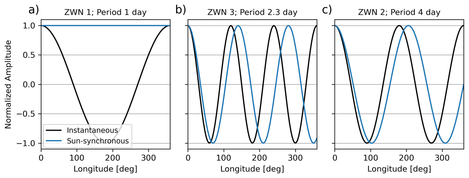
Figure 1 Sampling of global-scale waves from a sun-synchronous orbit for (a) DW1 solar tide (e.g. Oberheide et al., 2000), (b) quasi-two-day wave (e.g. Ern et al., 2013) and (c) a fast Rossby-wave mode (e.g. Salby, 1984). Black is the actual wave at t=0 and blue is the observed perturbation from the moving instrument accounting only for a single (e.g. ascending) orbit direction. Descending orbits would observe the system phase shifted depending on latitude.

The effect is most striking for the DW1 (Diurnal Westward-propagating zonal wavenumber 1 tide) and for a sun-synchronous orbit, where the orbit is fixed in space with a constant position relative to the sun. Since the satellite passes any latitude at fixed local time (differing between ascending and descending orbit), it always observes the same phase of the wave. Note that the tide is a true propagating wave mode driven by the sun that has a specific zonal wavenumber and frequency. Accordingly, at different altitudes, latitudes, or local times (e.g. ascending and descending orbit nodes) the observed phase is different. A helpful illustration can be seen in animation based on an NCAR tidal model (https://www.hao.ucar.edu/modeling/gswm/mwave2sm/movie.gif, last access: 30 January 2026) by Maura Hagan.

Deviations between instantaneous (or synoptic) sampling and time-varying (asynoptic) sampling of a satellite may be up to twice the amplitude for realistic scenarios. The waves can only be fully captured if in addition to the wavenumber, the frequency is also determined by a space-time spectral analysis. Taking this additional criterion into account, selecting the most suitable method for an instrument requires a thorough inspection of each background removal technique. This has been done for this study and is explained in detail in Appendix B. Based on careful examination of each method, we select the 2D spectral decomposition, which can deal with high zonal wave numbers (6–7) and frequencies up to 1 cycle d⁻¹ (considering both ascending and descending branches of a sun-synchronous or slowly precessing orbit), as the optimal method for background removal for a limb imaging satellite instrument. The presented implementation of the 2D spectral decomposition employs a Lomb-Scargle (Lomb, 1976; Scargle, 1982) approach, fitting the amplitudes of wave modes with frequencies from −1 to +1 cycle d⁻¹ and all integer zonal wavenumbers up to 7. The longest resolvable period is given by the length of the fitting window, which was chosen, for example, to 31 d in Ern et al. (2018).

This study gives a detailed algorithmic description of the background removal methodology using a planetary wave and tide fit. The accompanying software is published as open access along this paper (Rhode et al., 2025). The next section gives a brief overview of the different simulated satellite data sets that have been used for testing and verification in this study. Section 3 follows up with a detailed step-by-step description of the methodology. Results for verification and demonstration cases are given in Sect. 4. This includes PW spectra, large-scale temperature reconstructions, and GW isolation. Finally, Sect. 5 gives a wrap up of the findings and an outlook for future studies.

2 Data

The performance of the background removal method described in this study is assessed by comparing PW spectra and resulting residual temperature perturbations between Gaussian grid data and simulated satellite data. The spectral analysis of the model data is straightforward and can be done using standard Fourier analysis. The simulated satellite observations, on the other hand, need to be consistent with the (continuous) time of observation, which is achieved by evaluation of the PW spectra of the model grid data at the time and location of the satellite measurement. The basis for this analysis is the ECMWF ERA5 reanalysis (Hersbach et al., 2020) on 0.3° horizontal and 3 h time resolution. This allows for spatial resolution of gravity waves and time resolution of tidal modes. The vertical sampling of the data is 1 km.

In a first step, the reanalysis data is scale separated into large-scale background and GW residuals using the spatial technique described by Strube et al. (2020). This is done by performing zonal FFT at each altitude and latitude of individual snapshots in time to get the spectra. Each spectrum is smoothed using a third order Savitzky–Golay filter (Savitzky and Golay, 1964) in latitude (width 7.5°) and afterwards inverted to obtain the large-scale background of the temperature field. Subtracting this background from the reanalysis data temperature field gives us the GW perturbations. Next, the PW spectra of the model grid data are calculated by applying time-longitude Fourier transform on the large-scale temperature fields on time windows of 28 d. The GW fluctuations are taken from a single snapshot of the model data (here daily at 12:00 UTC).

Furthermore, we generate simulated satellite data as realistic test cases. In terms of observation grid, we use the specifications of 1 km vertical, 50 km along-track, and 25 km across-track resolution, which are the values of the ESA Earth Explorer 11 candidate CAIRT (Rhode et al., 2024) but are also representative of the NASA Earth System Explorer candidate STRIVE. The simulated swath width of the instrument is taken as 20 points across-track, i.e., roughly 500 km.

The simulated satellite data, which is given on continuous time along the orbit track, is determined by evaluating the PW spectra of the reanalysis at the time and location of the observation. This gives us the large-scale temperature variation accounting for the continuous measurements without discontinuities even though the model data is only present every 3 h. This can not be done for the GW perturbations since they are too fast to be resolved in time in the model data. Thus the GW perturbations are simply taken as daily snapshots from the model and sampled to the satellite observation grid. The GW perturbations are, therefore, discontinuous between observation days. However, since the GWs are of very short scales, this poses no problem for the scale separation approach. Note that we use two sets of simulated observations for testing: the time-continuous large-scale temperature background only and the same background with sampled GW perturbation added.

3 Algorithm description

The aim of the scale separation of a variable, i.e., temperature measurements from satellite orbit data in our case, is to isolate the global-scale background, which includes planetary waves and tides, from small-scale GW perturbations. The following approach on 2D spectral decomposition involves determination of the wave amplitudes and phases of different wave modes corresponding to each frequency and wavenumber over a specified time window. The resulting spectrum can then be used to reconstruct a large-scale approximation of the variable along the original spatio-temporal coordinates of the orbit. This section outlines the step by step procedure for performing the analysis on CAIRT temperature data, which consists of a fixed number of measurements across-track and measurements performed in regular time intervals. The methodology and analysis is, in general, also applicable for single track satellite data.

The general outline of the algorithm for fitting global-scale waves is shown as a flow chart in Fig. 2. The product of the methodology is a physically meaningful large-scale background that can be subtracted from the measurements to obtain temperature residuals that can be attributed almost entirely to perturbations due to GWs, i.e., “GW perturbations” or “GW residuals”, which can then be used for further analysis. Another, more technically detailed flowchart is shown in Fig. C1 in Appendix C.

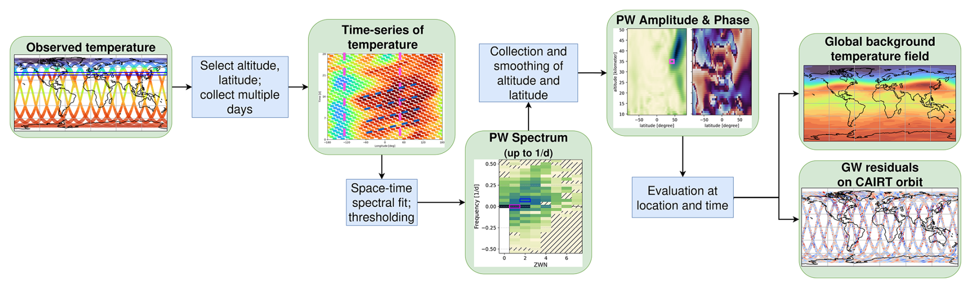
Figure 2 Illustrated flowchart of the global wave fit algorithm.

3.1 Pre-processing of the satellite data

The planetary wave spectrum describes waves in the time-longitude plane spanning full circles of fixed latitude around the globe. Therefore, the space-time decomposition is to be performed on a specified, regular grid of altitudes and latitudes. The satellite observations, on the other hand, are given on irregular points of longitude and latitude and, potentially, altitude. For observations on a fixed altitude grid, as in the case of the simulated CAIRT data, the first step before fitting the global-scale waves, is an interpolation to a fixed latitude grid. For this, every measurement track is interpolated independently to a predefined grid of latitude points using a cubic interpolation scheme. The measurement longitude and time are interpolated as well as the actual measured temperature. Technically, the satellite data is separated into individual orbit tracks, i.e., alternating ascending and descending segments, before the interpolation is performed. This results in a dataset that is given on an altitude-latitude fixed grid (in the following called ALF data; altitudes are determined by the instrument sampling or previous interpolation).

For the planetary wave and tide analysis, multiple days of ALF data are concatenated such that the time window is long enough to resolve propagating wave modes. Seasonal trends could negatively impact the spectral analysis by introducing a background floor that obscures the real amplitudes. Therefore, the last step of pre-processing is the removal of a linear trend in the zonal mean along each altitude-latitude point. In particular, only the linear component of the trend is subtracted to preserve the mean temperature (zonal wavenumber 0) for spectral analysis. In the following, the planetary waves are fitted on windows of 28 d while we use a window of 5 d for tides.

3.2 Global-scale wave fit

After the ALF data is generated, the global-scale wave spectrum is calculated using a standard method of least-squares optimization. In particular, for each point of altitude and latitude the full spectrum is fitted simultaneously by minimizing the cost function:

$$\begin{array}{}\text{(2)}& {\displaystyle }C(z,\mathit{\varphi })=\sum _i{\left(T_i-\sum _{n=\mathrm{0}}^{N_{\text{max}}}\sum _{\mathit{\omega }}A({\mathit{\lambda }}_i,t_i;n,\mathit{\omega })\right)}^{\mathrm{2}},\text{(3)}& {\displaystyle }\text{where}\text{(4)}& {\displaystyle }\begin{array}{rl}A& (\mathit{\lambda },t;n,\mathit{\omega })=\\ & {\widehat{A}}_{\mathrm{s}}(n,\mathit{\omega })\sin \left({\displaystyle \frac{n\mathit{\lambda }}{\mathrm{2}\mathit{\pi }}}-\mathit{\omega }t\right)+{\widehat{A}}_{\mathrm{c}}(n,\mathit{\omega })\cos \left({\displaystyle \frac{n\mathit{\lambda }}{\mathrm{2}\mathit{\pi }}}-\mathit{\omega }t\right).\end{array}\end{array}$$

The fitted parameters are the amplitudes of a sine and cosine wave, ${\widehat{A}}_{\mathrm{s}}(n,\mathit{\omega })$ and ${\widehat{A}}_{\mathrm{c}}(n,\mathit{\omega })$. n is the zonal wavenumber and ω the ground-based frequency of the wave. T_i, λ_i, and t_i are the observed temperatures, longitudes, and times of observation interpolated to the ALF grid, respectively. The maximum zonal wavenumber N_max is limited by the number of observations per day and should at most be half the number of daily orbits. The mean background corresponds to $k=\mathit{\omega }=\mathrm{0}$ (${\widehat{A}}_{\mathrm{s}}(\mathrm{0},\mathrm{0})$ is explicitly set to 0 and not fit). The phase of the wave mode is codified in the relation of the sine and cosine amplitudes. Note that it is important to fit all spectral modes simultaneously as they are no longer orthogonal if the observation points are not equidistant in space and time (which is in general not given for satellite observations).

This step results in spectra of global-scale waves, which may be further processed to, e.g., suppress unphysical modes due to aliasing of GWs, before further processing. For one, the fitted waves are expected to be highly correlated in latitude and altitude direction as they describe global wave modes of large extent. Therefore, a Savitzky-Golay (SG) filter in latitude and altitude is applied to the spectra. This removes strong jumps in the spectrum that could be introduced by, e.g., GWs of long horizontal wavelengths with east-west oriented phase fronts. From experience, third order polynomials work best in latitude smoothing. Vertical smoothing over the tropopause would, if applied at all, require fourth order polynomials. Typical smoothing width may be in the range of 5 to 15° latitude and 3 to 5 km in the vertical direction. The best choice would depend on many parameters (e.g. noise-level, track-width, along-track sampling) and to be optimized for the individual instrument.

The resulting PW spectrum obtained from the satellite observations containing only global-scale waves can then be evaluated on the initial observation grid to give a time-dependent large-scale temperature background. Subtracting this background from the full observations results in remaining temperature perturbations caused by small-scale GWs and tides. The tide removal is the aim of the next step in the processing.

3.3 Tidal signal removal

A satellite on a sun-synchronous orbit will pass a given latitude at fixed local times for ascending and descending orbits, respectively. Therefore, daily (and faster) tides are not resolved in time within the measurements but will be seen as static wave modes or constant biases separately for the ascending and descending orbit segments. In our tool, information about the phase and the actual amplitude can not be determined, but their signal can be removed from the observations nevertheless. Due to similar reasoning, eastward and westward propagating tides are indistinguishable.

To characterize the tidal signal, we perform a second wave fit using the results of the last processing step, i.e., observed temperature minus the planetary-wave background. It is from these temperature differences on the orbit grid, separated into ascending and descending orbit segments, that tide spectra are obtained from. The cost function to be optimized looks analogously to Eq. (2) but contains only constant modes, i.e., ω=0:

$$\begin{array}{}\text{(5)}& {\displaystyle }C(z,\mathit{\varphi }){\displaystyle }=\sum _i{\left((T_i-T_{\text{PW},i})-\sum _{n=\mathrm{0}}^{N_{\text{max}}}A({\mathit{\lambda }}_i,t_i;n,\mathrm{0})\right)}^{\mathrm{2}}.\end{array}$$

Here, T_PW,i are the temperatures generated by evaluating the PW spectrum from the previous step.

Due to the simultaneous propagation of the tides and the satellite orbit, the fitted wave modes will be shifted by one wave number: the migrating diurnal tide (DW1), for example, is seen at n=0. Furthermore, this way of indirectly capturing tides is performed using a shorter time window (e.g., 5 d) as done by Ern et al. (2018), which allows amplitudes to vary at the time scale of the window length. The tide processing has to follow the planetary wave fits in order to address the quasi-stationary modes properly. The resulting tide spectra (differing for ascending and descending orbit segments) can then be evaluated on the observation grid, and subtracted from the residuals of the previous processing step to yield the small-scale GW perturbations.

3.4 Processing of long time series

For long-time observations and further analyses, the methodology is applied as follows: starting with multiple months of (simulated) satellite observations of temperature, the planetary wave analysis and background generation is performed on moving, fixed-length time window of 28 d. The analysis window is shifted across the whole analysis period by increments of constant size depending upon the total analysis length (one day in this study, which might not be reasonable for datasets that span several decades). The PW spectra are considered to be most reliable for the central day(s) of the analysis. From these, the large-scale background temperatures are calculated and removed by evaluating the spectra at the given time. Likewise, the tidal removal is performed in a shifting window, leaving us with just the GW residuals. For all but the days at the edge of the considered period, the spectrum centered on the given day is used for the evaluation of the background temperature.

4 Results

Although the final aim of the described scale separation are the small-scale temperature residuals caused by GWs, there are a few other aspects that can be looked at. In this section, we estimate the performance of the scale separation but also show some not directly related results like PW spectra for analysis and a global background temperature field beyond the limitations to the observation grid.

4.1 Temperature fields

Before we go into the details of the performance, Fig. 3 shows an example of the input data for a single snapshot of the model or a day of simulated observations, respectively. Note that the simulated observation is time-dependently sampled, which can be seen in the discontinuities where the ascending and descending orbits cross. In particular, this is visible around 40° W, 30° N. The GW residuals shown in Fig. 3d, on the other hand, are directly sampled from the snapshot and fully resemble the model residuals in Fig. 3b.

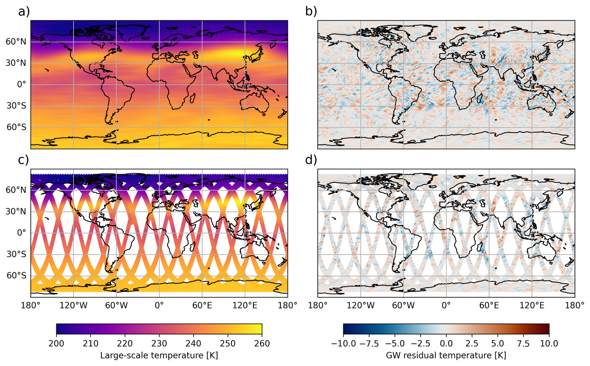
Figure 3 Example of the prepared test data for 24 January 2019. The upper row shows the model temperature large-scale background (a) and GW residuals (b) as the snapshot at 12:00 UTC. The bottom row shows the simulated observations of the (time-dependent) large-scale background as evaluated from the model PW spectrum (c) and the sampled GW residuals (d).

4.2 PW spectra

An example of a PW spectrum as generated from simulated satellite observations and directly from the model data is shown in Fig. 4. Note that the spectrum from the observations is limited to frequencies slower than 1 d⁻¹ and that the spectra are calculated form the large-scale background without GW perturbations. Furthermore, the effect of the Savitzky-Golay filtering on the PW spectrum is shown. Overall, the model spectrum is very well reproduced in terms of dominating wave modes and their amplitudes: the 99th percentile of absolute amplitude deviation is smaller than 0.3 K globally. There are, however, also some more spread out deviations between the reference and the satellite observations. For example, at high zonal wavenumber and high negative frequency, the spectrum from the satellite data shows some spurious amplitudes. These are caused by aliasing of higher frequency waves that cannot be resolved with the satellite sampling. This includes, in particular, the semi- and terdiurnal tides. Nevertheless, the amplitudes of the spurious wave modes are comparatively low at below 0.1 K and, therefore, do not lead to problems in the scale separation. Higher absolute deviations from the reference are found for wave modes with higher amplitudes, especially for the mean, i.e., ZWN 0, $f=\mathrm{0.0}{\mathrm{d}}^{-\mathrm{1}}$, where absolute deviations of up to 5 K are found. In general, however, the relative deviation to the reference amplitudes is below 2 % for components with amplitudes higher than 1 K.

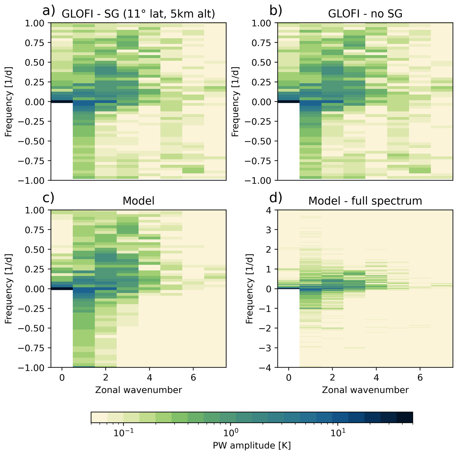
Figure 4 Comparison of the determined PW spectrum from the GLOFI algorithm applied to simulated satellite observations with and without Savitzky-Golay filter (a and b, respectively) and the reference spectrum calculated from the full model data in the satellite-observed frequency range (c) and the full spectrum (d). The PW spectrum of the model includes higher frequencies up to 4 cycles d⁻¹, which cannot be inferred from the satellite observations and are (at least partially) aliased into the GLOFI spectra. The spectrum is shown for the time window of 16 January 2019 to 12 February 2019 at 40 km altitude and 60° N.

Figure 5 shows the PW amplitude and phase of a single wave mode across the whole altitude and latitude range as an example. The structure of both the amplitude and phase determined from the simulated satellite observations agree very well with the ones from the full model data. Even small-scale variations of the amplitudes are well represented in the satellite data. The GLOFI methodology finds large-scale coherent wave structures throughout the atmosphere just as present in the reference data. Applying the Savitzky-Golay filter has a rather neutral effect on the PW spectrum: some regions fit better to the model data, others minimally worse. This and the good agreement to the model data give confidence that the methodology describes the PW situation within the atmosphere realistically.

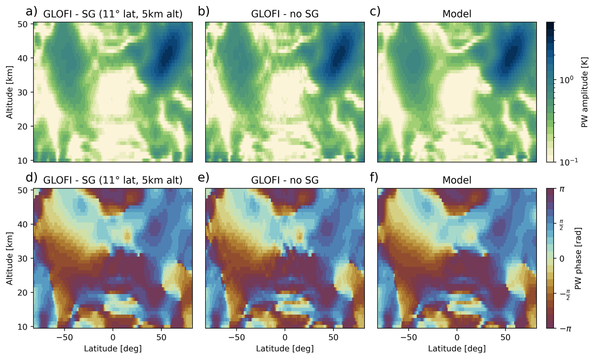
Figure 5 Comparison of amplitude and phase for the PW with zonal wavenumber 1 and frequency of $-\frac{\mathrm{3}}{\mathrm{28}}$ cycles d⁻¹ (9 d period) as determined by GLOFI with (a, d) and without Savitzy-Golay filtering (b, e) and from the full model data  (c, f). The data shows the spectrum for the time window 16 January 2019 to 12 February 2019.

The deviations of the GLOFI processing to the model reference is further detailed in Appendix D.

4.3 Reconstructed background

Evaluating the spectra along the satellite observations in time and longitude gives the temperature background, which can be subtracted from the observed temperatures to yield small-scale perturbations. Sometimes, however, a large-scale temperature background might also be useful, e.g., for ray-tracing applications. Here we compare the performance of the background reconstruction on orbit data and showcase the possibility to reconstruct a background on a global grid.

4.3.1 Satellite orbit

Figure 6a and b show an example of simulated temperature observations of an atmosphere without GWs and the estimated background reconstructed from the planetary wave spectrum. The shown situation is reconstructed at the central date of the analysis window used for the PW spectrum shown in Sect. 4.2. The reference observation and the reconstruction are indistinguishable from each other. For a more quantitative comparison, Fig. 6c shows the difference between both data sets. The remaining temperature differences are very small and well below the amplitudes of typical GWs. These residuals occur mostly due to the aliasing of higher frequency planetary modes to the resolved spectrum of the satellite (which was confirmed by spectral analysis of the reconstructed temperature from the grid spectrum truncated to the observable frequency range – not shown). The differences between reference and reconstruction are approximately Gaussian distributed around zero with a standard deviation between 0.05 and 0.2 K, increasing with altitude.

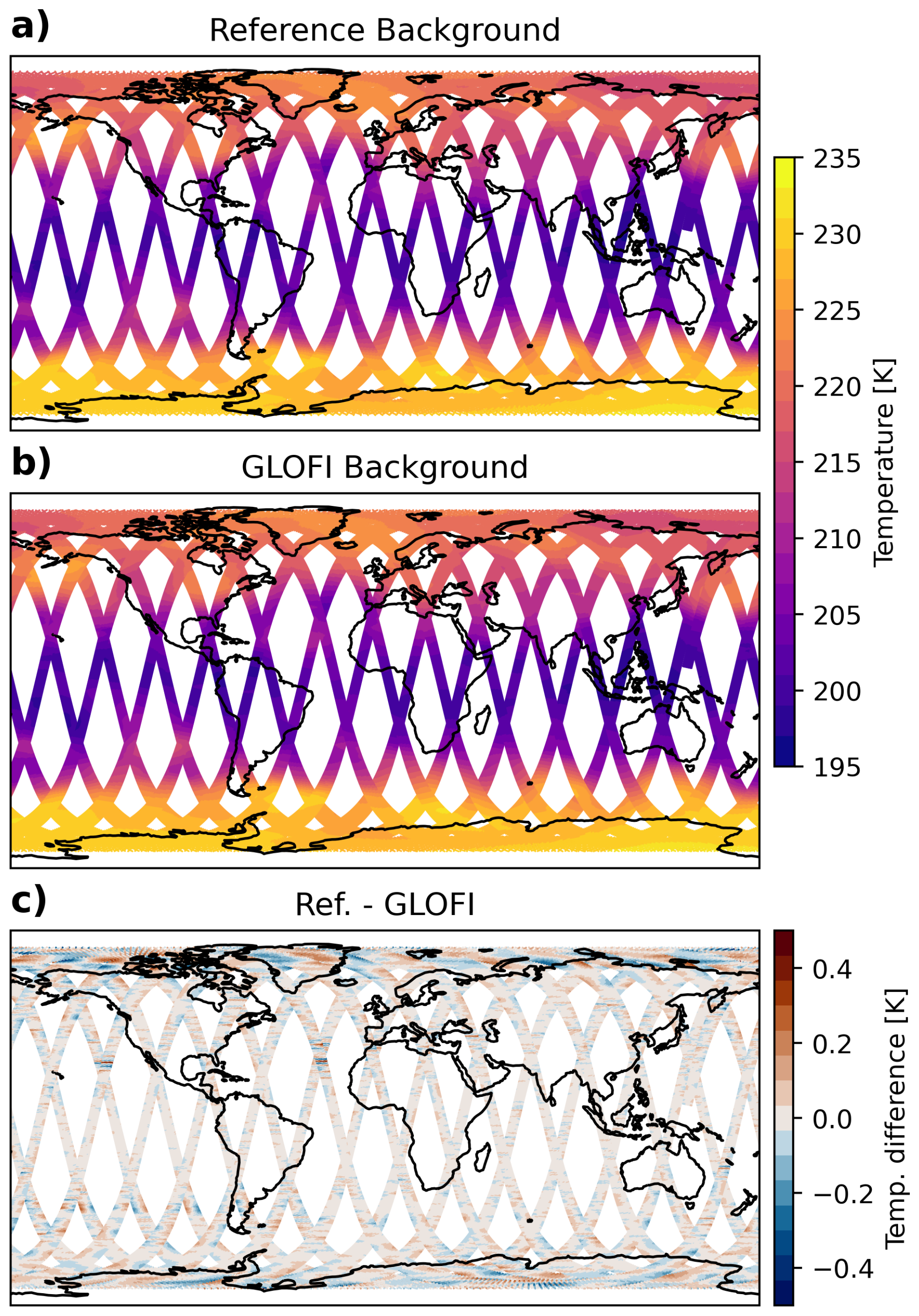
Figure 6 Global temperatures as from a simulated observation of the satellite grid-sampled large-scale background (a) and a reconstruction from the GLOFI PW spectrum (b) and the difference between both (c). Shown is 30 January 2019 at 15 km altitude.

4.3.2 Global grid

The planetary spectra determined from the satellite observations describe global-scale waves and can, hence, also be used to reconstruct a global temperature field. In this way, a satellite can observe an approximated global temperature field even though it has gaps in between the orbits. The tides, however, are not accounted for as these are not easily reconstructed due to the lack of phase information on the observation grid, as discussed in Sect. 3.3.

Figure 7 shows an example of the quality of this approximation. As can be seen, the general structure and features are reconstructed very well, while the exact temperature values are off by up to 3 K. The deviations are comparatively local and small in comparison to the absolute temperatures. Even though this is not the primary aim of the methodology, this would be a valuable byproduct for, e.g., raytracing (in combination with geostrophic winds) or as a first approximation of a global temperature field as alternative to, e.g., an assimilation system.

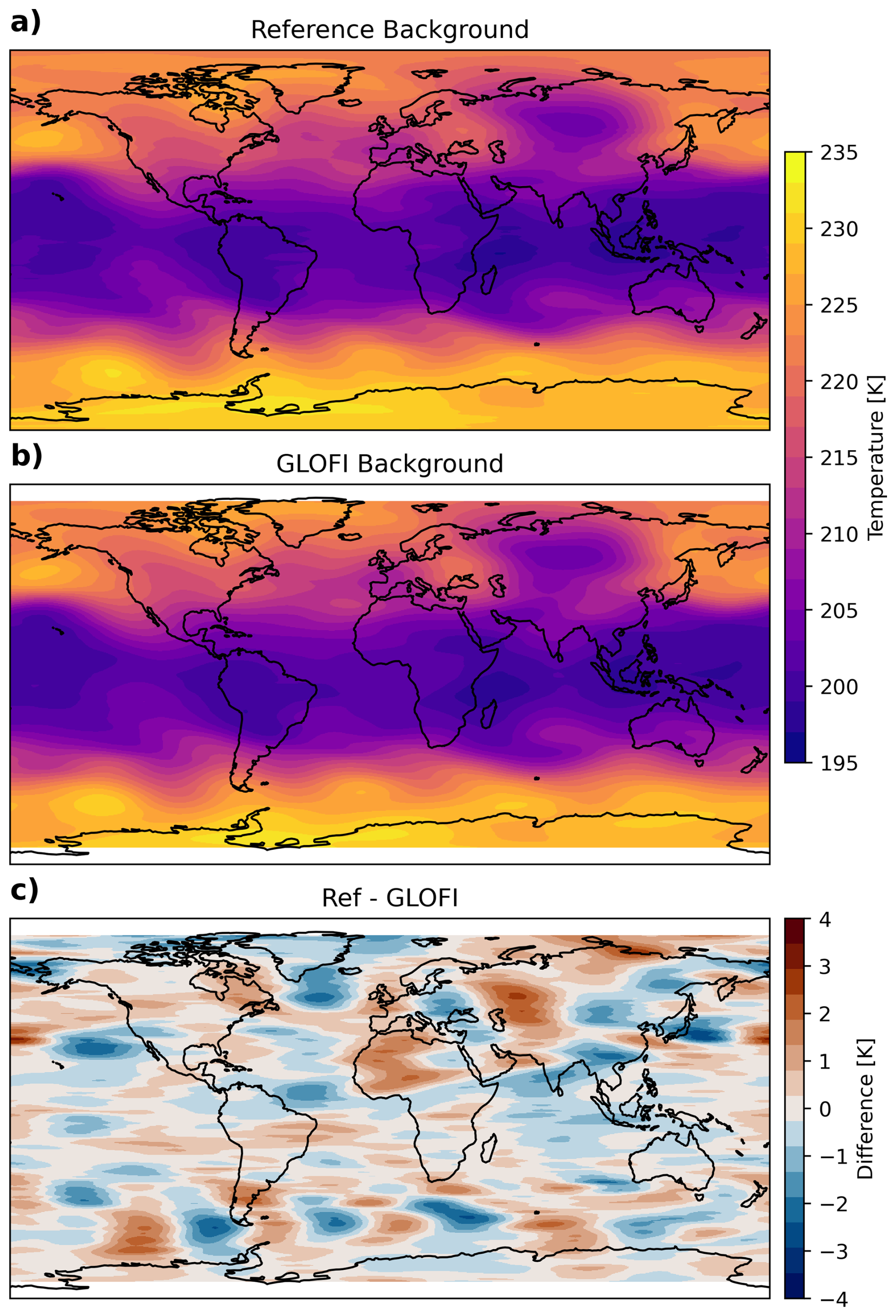
Figure 7 Temperature background from model data (a) and reconstructed from the GLOFI PW spectrum shown in 4.2 (b) as well as the difference between both (c). Shown is 16 January 2019, 00:00 UTC at 15 km altitude. Note that the differences are mostly due to the lack of tides.

4.4 Residual temperatures

For the performance evaluation of the actual scale separation into PW background and GW perturbations, we use synthetic observations containing the simulated background as well as sampled GWs of a single model snapshot and apply the GLOFI algorithm to generate the PW and tide spectra. The resulting spectra are then used to reconstruct the large-scale temperature background at the satellite orbit coordinates. The difference between the background temperature thus obtained and the synthetic observations yields the GW perturbations on the satellite grid. A comparison of these GW perturbations to the satellite-sampled GW perturbations of the model allows the estimation of the algorithm performance for realistic observations. Figure 8 shows an example of such a comparison. The differences between the sampled reference (Fig. 8a) and GLOFI-recovered GW perturbations (Fig. 8b) is shown in Fig. 8c. The differences have a zero mean with a standard deviation of 0.02 K. The regions of higher deviations, where differences go to a maximum of 0.29 K, coincide with latitudes at which the GLOFI estimated background deviate strongest from the reference, as shown in Fig. 6c. As discussed, these show up due to to aliasing from higher frequency planetary modes.

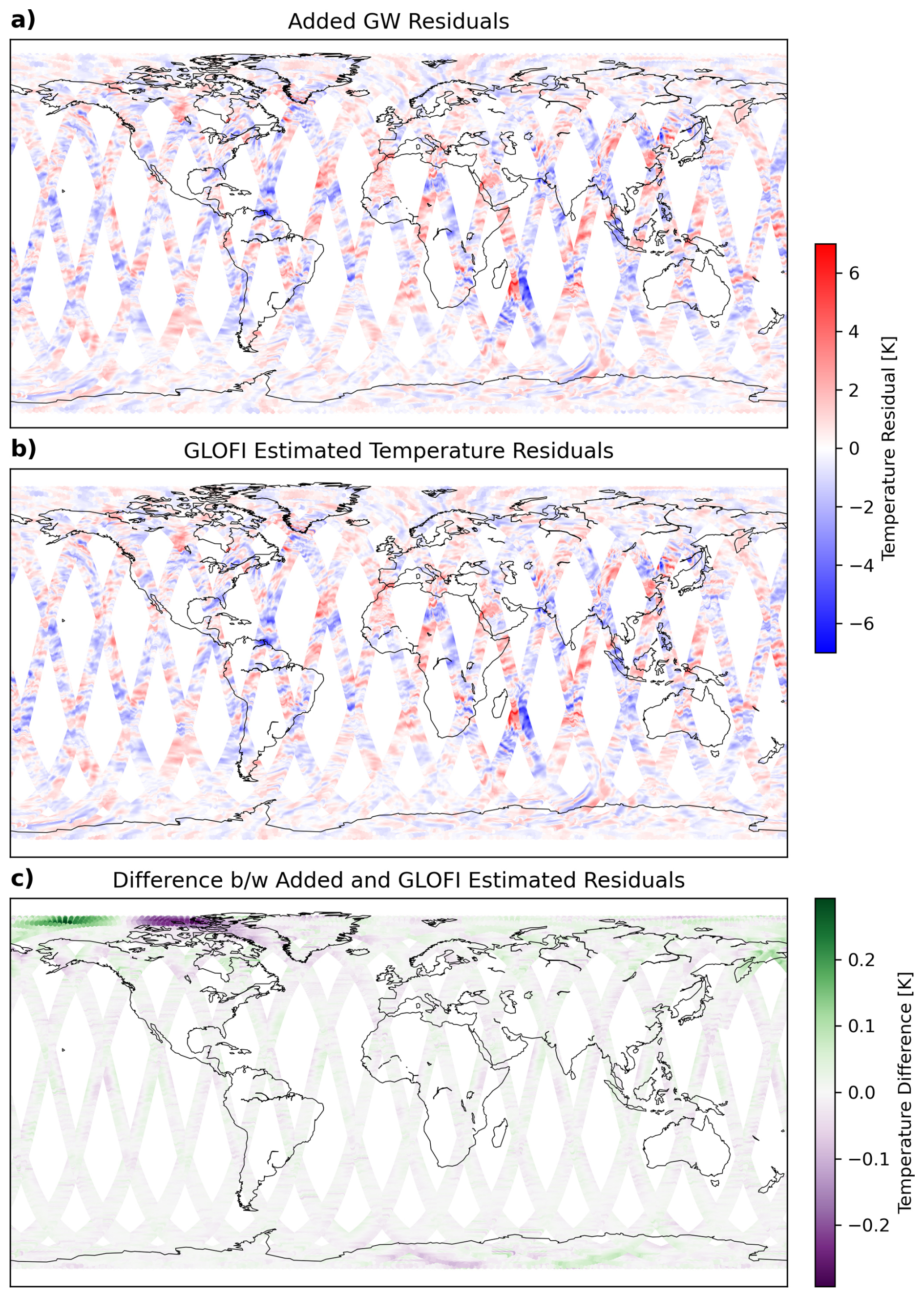
Figure 8 GW residuals as sampled from the model (a), as determined from the GLOFI algorithm (b) and the difference between the two (c) at 35 km altitude for the day 20 January 2019.

4.5 Temperature variances

To estimate the performance of the background generation methodology, we compare the variances of the GWs and the PWs in Fig. 9. The GW perturbations show lower variances than the PWs, especially at higher latitudes. The scale separation must remove the PW background in a way such that the variance of the residual temperature differences, such as those shown in Fig. 6c, are much smaller than those of possible GW perturbations. In this way, we can make sure that the GW perturbations dominate and can be well analyzed. Hence, Fig. 9 also shows the variances of the difference between the satellite-observed (i.e., just sampled) temperature background and background generated by the GLOFI methodology. In this case, the wave fit was performed for zonal wavenumbers up to 7 and 56 frequencies within the Nyquist limit.

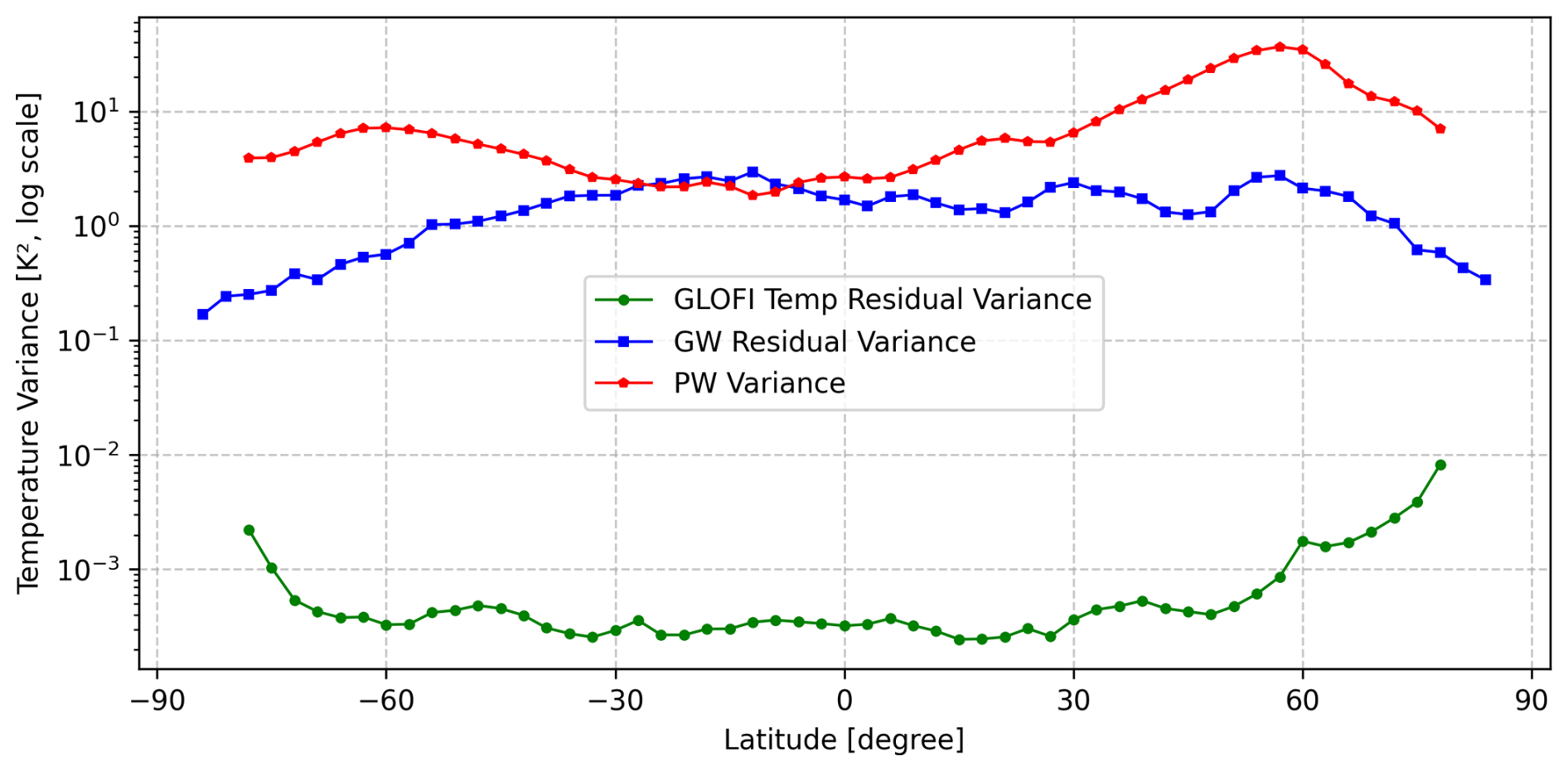
Figure 9 Temperature variances of (sampled) GW perturbations, PW perturbations and remaining residuals after subtracting the GLOFI PW background from the PW residuals at different latitude points. Shown is data for 12 March 2019 at 25 km altitude.

As can be seen, the remaining variances are orders of magnitude smaller than the variances of the GWs, which shows that the background removal performs well in order to suppress the PW background below the GW perturbations. In particular, the remaining residuals that are beyond the resolving capabilities of the satellite sampling are much smaller than the GWs and do not interfere with their analysis.

5 Conclusion

The analysis of GWs within observations can usually not be done straightforwardly as the observations contain signals of different physical effects, obscuring the GW signal within the data. Therefore, a method of scale separation is necessary to isolate the GW signal. Depending on the observation technique, there are multiple possible methods to achieve this. For limb scanning satellite instruments, particularly if they fly on a sun-synchronous orbit or other slowly-precessing orbits, the method of fitting a global-scale background based on planetary wave perturbations is best suited. In particular, the 2D spectral decomposition by fitting of time- and longitude-varying wave modes is possible for satellite observations.

Here, we have presented a methodology that achieves the scale-separation by fitting the planetary wave modes in two steps: a first step describing the constant and time-varying modes followed by a second fit for the tides, which are harder to access from a sun-synchronous orbit and require the separation of ascending and descending orbit segments. In both cases, we employ a simultaneous least squares fit of all wave modes. In case of the tides, only static modes are fitted, as the solar local time of crossing a given latitude is constant (but different between ascending and descending nodes).

We have demonstrated the performance of this methodology using simulated temperature observations of the ESA Earth Explorer 11 candidate CAIRT as test case. With a vertical resolution of 1 km and a swath width of 300–500 km, it is well suited for observing GWs in the atmosphere once the large-scale background is subtracted.

The performance estimation shows that the methodology is very capable of recovering the PW spectra of the model data that have been used for generating the simulated observations. Evaluating the PW and tide spectra on the observation grid results in the large-scale background. Subtracting this from the full observations yields the temperature perturbations caused by GWs for further analysis. As we have shown, the methodology suppresses the PW and tide contributions to the observations much below the GW perturbations.

A realistic test case using simulated, time-dependent background temperature observations and sampled GW residuals shows that the methodology indeed yields realistic and unperturbed GW residuals compared to the input GW residuals. I.e., the PW and tide spectra are not strongly influenced by the small-scale perturbations.

Summarizing, the presented methodology presents a fully functional and tested toolbox for the scale separation of satellite observations. Applying the methodology to GNSS-RO temperature observations is a planned follow-up study. The toolbox will be published as open-access code alongside this article as the GLOFI project.

Appendix A: Overview on Background removal techniques

Global wave modes contribute to the observed temperature values at the locations where they are found. Hence, to extract information about the GWs, which are much shorter in scale, from any kind of observations, the initial step involves separating the GWs from the background temperature, which includes the mean background values as well as global wave modes like planetary waves. This scale separation can in principle be performed vertically, horizontally or temporally. For temporal background retrieval, monthly or seasonal mean observations have to be calculated, which is only viable for fixed-location, ground based measurements. For vertical background retrieval from either type of measurement, polynomial fits of the vertical profile can performed, (Allen and Vincent, 1995; Vincent and Alexander, 2000; Wang and Geller, 2003; Pramitha et al., 2016; Zhang and Yi, 2005, 2007; Zhang et al., 2010). The order of the polynomial is chosen based on the desired vertical wavelength, with higher-order polynomials progressively filtering out shorter-scale perturbations. But polynomials of order greater than four can remove perturbations associated with the inertia GWs in the profiles (Guest et al., 2000).

Spectral filtering (Hirota, 1984; Eckermann et al., 1995; Tsuda et al., 2000; Hirota and Niki, 1985; Ehard et al., 2015) can be used to identify or separate waves of specific wavelengths from measurements containing a spectrum of waves. For instance, high-pass filters are applied in the time domain to eliminate the low-frequency components of other large-scale waves, and in the height domain to remove contributions from tides and planetary scale waves. A low-pass filter is used in the height domain to filter out shorter wavelengths, while a band-pass filter can be employed to isolate the wavelength of interest by cutting off both the lower and higher ends of the wavelength spectrum. Note that the vertical filtering struggles with removing Kelvin waves in the tropics due to their vertical wavelengths being similar to those of GWs.

To examine the localized variations of different waves along with the frequency information, wavelet analysis is often employed. This approach decomposes a time series into time-frequency or position-frequency space, enabling the identification of dominant modes of variability and their temporal or spatial fluctuations. In wavelet analysis, signals are broken down into shifted and scaled versions of a base function known as the mother wavelet. A commonly used mother wavelet is the Morlet wavelet, which consists of a plane wave modulated by a Gaussian envelope (Zink and Vincent, 2001).

Removal of global wave modes from satellite data has been performed in many studies using a variety of methods, including some of the methods discussed previously. Two-dimensional spectral decomposition, described in Ern et al. (2011), resolves global-scale waves with zonal wave numbers up to 6–7 with periods as short as 1–2 d. This method involves a spectral decomposition along the dimensions of longitude and time to identify shorter period planetary scale waves. Utilizing this technique, Ern et al. (2011) leveraged observations from HIRDLS and SABER to study global Gravity Wave momentum flux (GWMF) from the stratosphere to the mesosphere.

Another technique which has been extensively used to separate gravity waves from background is the Kalman filter. The background atmospheric conditions are typically modeled using 0–6 wavenumber zonal planetary wave temperature coefficients, estimated through a Kalman filter. For example, Ern et al. (2006) conducted a comparison study of GWMF between observations (CRISTA-1 and CRISTA-2) and model analyses using the Warner and McIntyre parameterization scheme (Warner and McIntyre, 2001), employing the Kalman filter to establish the atmospheric background from instantaneous observations. Fetzer and Gille (1994) removed planetary waves 0–6 using this method.

A spectral analysis technique similar to the wavelet transform, the Stockwell transform, is based on modulating signals with a Gaussian width inversely proportional to the wavelengths.This approach was effectively utilized by Alexander et al. (2008) and Wright et al. (2010), who applied the S-transform to analyze temperature perturbations of GWs from HIRDLS/Aura. Alexander et al. (2008) finds wave numbers 0–3 planetary-scale zonal oscillations using Stockwell transform and removes them from HIRDLS temperature measurements.

Finally, a local horizontal filtering method was applied to AIRS data (Hoffmann and Alexander, 2010), which has the advantage of being able to estimate a background at the time of the observation and thus remove large-scale waves of all periods including fast planetary waves and tides. This, however, requires a wide swath width for giving reliable results.

Appendix B: Choice of background removal technique

The task of removing global-scale waves from data in order to isolate the localized temperature structures of GWs is challenging. Moreover, the amplitudes of typical planetary wave modes are larger than typical GW amplitudes by roughly one order of magnitude. The most severe deviations due to sampling (as seen in Fig. 1) are not necessarily the most harmful ones: the aliasing from one planetary wave mode to a constant value or a stationary planetary wave mode for solar tides if ascending and descending orbit data are treated separately is actually advantageous in removing the tides before GW analysis, as will be seen later in Sect. 3.3. Though less dramatic, the deviations seen for other fast, i.e., high frequency, planetary wave modes are far more problematic. Table B1 provides a list of the different background removal methods, the satellite datasets used in studies applying each method, as well as the corresponding horizontal and vertical wavelength ranges covered. It should also be noted that the regions of GW wavelengths and frequencies that are visible depend on the instrument design as well. An overview of the general regions of the GW spectra that is observed by different measurement techniques is given in Fig. 8 of Alexander et al. (2010) and Fig. 9 of Preusse et al. (2008). For the observable spectrum of the CAIRT instrument used in this study, refer to Rhode et al. (2024). Additionally, the drawbacks of each method, as documented in various studies, were also considered to identify the most suitable one for our purposes. For instance, motivated by inertial instability signals in GNSS-RO data (Rapp et al., 2018), Strube et al. (2020) compares horizontal and vertical filtering methods to remove large-scale background from ERA5 reanalysis temperatures, a synthetic dataset and 1 year of SABER temperature data. For vertical filtering, the threshold wavelength which has to be set to remove the global waves as well as inertial-instability-like perturbation eliminates a major part of the gravity wave spectrum as well. Meanwhile, horizontal filtering was able to retain GW information after applying a horizontal cutoff wavenumber of 6, which removed inertial instabilities as well as Kelvin waves and stratopause remnants.

The different horizontal filtering methods do, however, have their own limitations. For example, the S-Transform fails to account for the temporal variations of large-scale waves, rendering it unsuitable for the removal of time-dependent waves. The removal of global scale propagating waves can be achieved using a local horizontal filter, a Kalman filter, or a 2D spectral decomposition. Applying a local horizontal filtering limits the longest horizontal wavelengths to values substantially shorter than the horizontal filter width (cf. Table B1: 1000 km max. wavelength compared to 1650 km AIRS wide measurement swath). In general, such a filter could be applied either along-track or across-track if the satellite has a non-zero swath width (e.g. Yan et al., 2010) but due to the preferred orientation of GWs in north-south orientation, a filtering in the across-track direction is usually favoured for GW analyses. For a across-track swath width of 300–500 km, which corresponds to the currently proposed satellite missions CAIRT (ESA Earth Explorer 11 candidate) and STRIVE (NASA Earth System Explorers Program candidate), this would result in limiting the maximum horizontal wavelengths to 180–300 km, and thereby remove a large fraction of the GW spectrum. Background removal using a Kalman filtering, on the other hand, cannot remove rapidly varying planetary waves of low zonal wavenumber (Fetzer and Gille, 1996).

A 2D space-time decomposition of the global-scale waves, however, can deal with high zonal wave numbers (6–7) and frequencies up to 1 cycle d⁻¹ (considering both ascending and descending branches of a sun-synchronous or slowly precessing orbit).

Table B1 Overview of different satellite observations and the respective background-removal techniques applied.

Appendix C: Technical flow chart

The GLOFI processing chain is detailed in Fig. C1. This includes all processing steps of the methodology.

Figure C1 Technical flowchart of the global wave fit algorithm.

Appendix D: PW fitting deviations

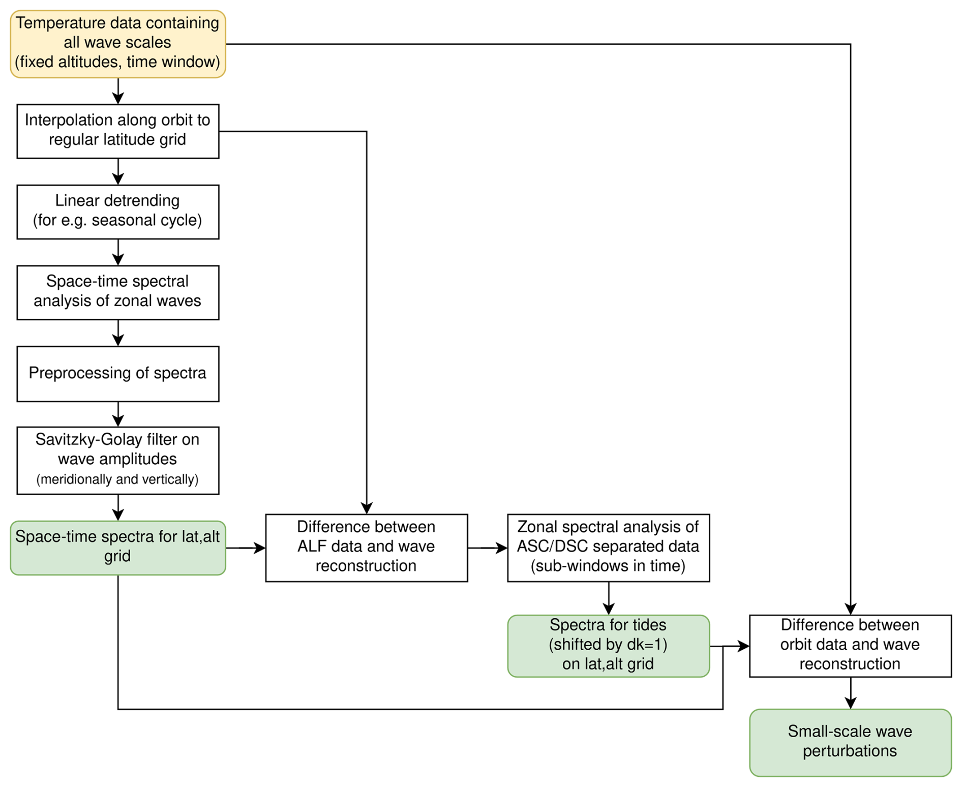
Figure D1 shows the deviations of the fitted PW amplitudes and phases in Fig. 5a, b, d, and e to the reference directly estimated from the model grid shown in Fig. 5c and f. In general, the deviations are very minimal even where the PW amplitude is very strong in the northern upper stratosphere. The phases are well recovered as well wherever the amplitude is high enough to give enough signal for the fitting (here around 0.3 K seems to be sufficient for the algorithm).

The application of the Savitzky-Golay smoothing filter (11° in latitude, 5 km in altitude) leads to smoothed deviations overall. However, it also deteriorates the performance of the algorithm around the tropopause. This can mostly be attributed to the vertical smoothing. Therefore, if your main interest is the upper troposphere/lower stratosphere, the Savitzky-Golay filter should limit to the meridional direction.

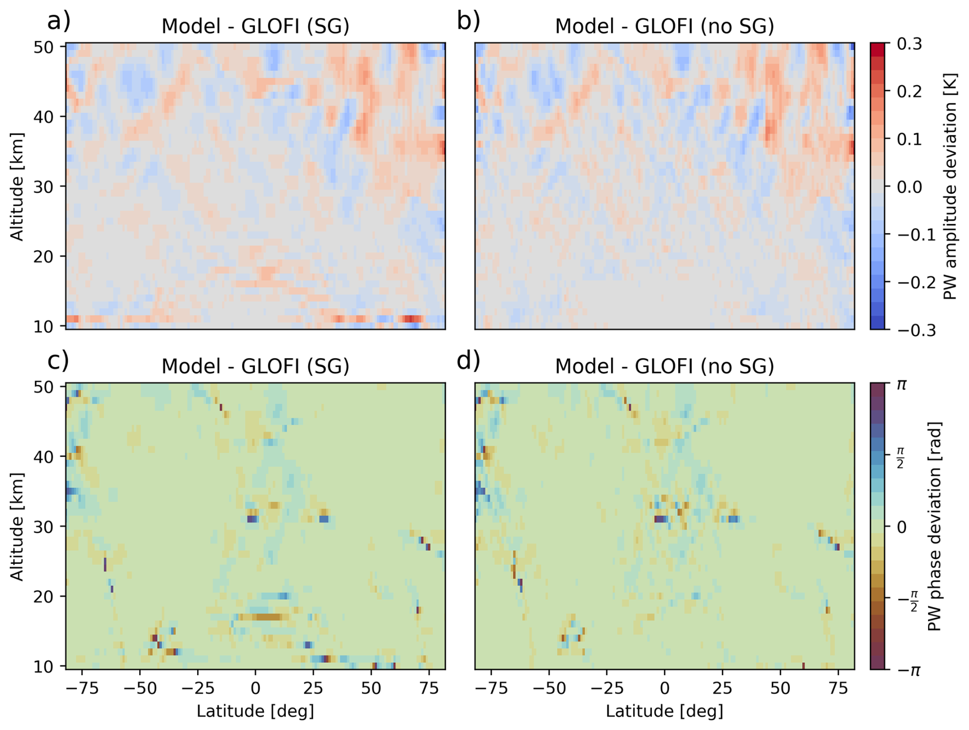
Figure D1 Difference in PW amplitude (upper row) and PW phase (lower row) between the reference estimated from the model and the GLOFI algorithm. Left and right columns show the corresponding deviations with and without the Savitzky-Golay filter applied.