Importance of interpolation and coincidence errors in data fusion

The complete data fusion (CDF) method is applied to ozone profiles obtained from simulated measurements in the ultraviolet and in the thermal infrared in the framework of the Sentinel 4 mission of the Copernicus programme. We observe that the quality of the fused products is degraded when the fusing profiles are either retrieved on different vertical grids or referred to different true profiles. To address this shortcoming, a generalization of the complete data fusion method, which takes into account interpolation and coincidence errors, is presented. This upgrade overcomes the encountered problems and provides products of good quality when the fusing profiles are both retrieved on different vertical grids and referred to different true profiles. The impact of the interpolation and coincidence errors on number of degrees of freedom and errors of the fused profile is also analysed. The approach developed here to account for the interpolation and coincidence errors can also be followed to include other error components, such as forward model errors.

1 Introduction

Many remote sensing observations of vertical profiles of atmospheric variables are obtained with instruments operating on space-borne and airborne platforms, as well as from ground-based stations. Recently, the complete data fusion (CDF) method (Ceccherini et al., 2015) was proposed for use in the combination of independent measurements of the same profile in order to exploit all the available information and obtain a comprehensive and concise description of the atmospheric state. This is an a posteriori method that uses standard retrieval products. With simple implementation requirements, the CDF products are equivalent to those from a simultaneous retrieval, considered to be the most comprehensive way of exploiting different observations of the same quantity (Aires et al., 2012), in spite of a greater computational complexity. However, so far, the data fusion method was mainly applied to measurements performed by the same instrument while sounding the same air sample.

Limited tests were conducted on measurements performed by different instruments when inconsistencies due to differences in the observed true profiles (because of the non-perfect coincidence of the space–time location of the measurements) could degrade the optimal performances of the simultaneous retrieval. About the fusion of data provided by different instruments, it has been proved (Ceccherini, 2016) that the CDF method is completely equivalent to the measurement space solution (MSS) data fusion method (Ceccherini et al., 2009). The latter was successfully applied to the data fusion of MIPAS-ENVISAT and IASI-METOP measurements (Ceccherini et al., 2010a, b) and of MIPAS-STR and MARSCHALS measurements (Cortesi et al., 2016). However, since in these cases the measurements to be fused (referred to as fusing profiles hereafter) carried information about basically complementary altitude ranges, their possible inconsistency did not result in unrealistic fused profiles.

The first applications of data fusion were made with profiles retrieved on the same vertical grid. A first analysis of the effect of different grids on the quality of the fused products was performed and presented by Ceccherini et al. (2016). In this case, the individual profiles were first obtained on grids optimally defined according to the information content of the individual observations. Then, the CDF method was performed using averaging kernel matrices (AKMs) interpolated to a common grid optimized for the data fusion product. Compared to the case in which the individual retrievals are obtained directly on the grid optimized for the data fusion, the number of degrees of freedom (DOF) is reduced by about a quarter with this approach. Thus, in data fusion applications the choice of the retrieval grid can lead to an information content loss that cannot be restored with interpolation.

Here, we consider the general problem posed by the application of the CDF method to measurements performed by different instruments that are retrieved on different vertical grids and refer to different true profiles (which correspond to the case of fusing profiles measured in different geolocations). The analysis of this problem suggests a modification of the CDF method, taking into account interpolation and coincidence errors. We determine the expressions of these errors and show how they enter in the CDF formula. The study is performed using simulated measurements of ozone profiles obtained in the ultraviolet and in the thermal infrared in the framework of the Sentinel 4 (S4) mission (ESA, 2017) of the Copernicus programme (http://www.copernicus.eu/main/sentinels). The advantages in using a multispectral approach for observing ozone profiles from space have been studied, using simulated measurements, by Landgraf and Hasekamp (2007), Worden et al. (2007), Natraj et al. (2011), Hache et al. (2014) and Costantino et al. (2017), and, using real measurements, by Fu et al. (2013) and Cuesta et al. (2013). Two review papers on this subject are Lahoz et al. (2012) and Timmermans et al. (2015).

The paper is organized as follows: Section 2 presents an account of the problems that occur when the CDF method is applied to vertical profiles retrieved on different vertical grids and referring to different true profiles. In Sect. 3, we theoretically analyse the problems discussed in Sect. 2 and show how the CDF method can be modified to overcome them. In Sect. 4, we show how the solution proposed in Sect. 3 solves the problems discussed in Sect. 2. In Sect. 5, we describe how to deal with forward model errors. Conclusions are drawn in Sect. 6.

2 Application of the CDF method to profiles retrieved on different vertical grids and related to different true profiles

The future atmospheric Sentinel missions of the Copernicus programme (http://www.copernicus.eu/main/sentinels) will provide great scope and a real test bed for data fusion applications. The wealth of data that will become available from these missions will likely present technical challenges to many applications. With the use of data fusion, the number of products can be reduced while maintaining the information content of the original datasets. For this reason, we test the CDF method on simulated data of the S4. We simulate two S4 ozone vertical profile measurements as they could be obtained from the Infrared Sounder (IRS) in the thermal infrared and from the Ultraviolet, Visible and Near-Infrared Sounding (UVN) spectrometer in the ultraviolet (http://www.eumetsat.int/website/home/Satellites/FutureSatellites/MeteosatThirdGeneration/MTGDesign/index.html) on board the MTG (Meteosat Third Generation) satellite. We refer to these two simulated measurements as TIR measurement and UV measurement, respectively.

In order to evaluate the effect of the variability of vertical grids and of true profiles, three cases are considered:

1. The simulated measurements refer to the same true profile and are retrieved on the same vertical grid.

2. The simulated measurements refer to the same true profile but are retrieved on different vertical grids.

3. The simulated measurements refer to different true profiles and are retrieved on the same vertical grid.

In all three cases, the true profile and the vertical grid of the UV measurement are kept fixed and, when pertinent, are changed for the TIR measurement. For simplicity, we define the vertical grid of the data fusion product to coincide with the fixed grid of the UV measurement. In the following, the vertical grid of the fusion product is referred to as the fusion grid.

For a meaningful comparison of the quality of fusing and fused profiles, it is necessary to have common a priori profiles and common a priori covariance matrices (CMs). Therefore, the a priori of the fusing profiles, which are produced with individual a priori assumptions, have been modified using the method described in Ceccherini et al. (2014). In the comparisons, the same a priori profiles provided by the McPeters and Labow climatology (McPeters and Labow, 2012) are used for all fusing and fused profiles. The a priori CMs are obtained using the standard deviation of the McPeters and Labow climatology when its value is larger than 20 % of the a priori profile and a value of 20 % of the a priori profile in the other cases. The off-diagonal elements are calculated considering a correlation length of 6 km. The correlation length is used to reduce oscillations in the retrieved profile and the value of 6 km is typically used for nadir ozone profile retrieval (Liu et al., 2010; Kroon et al., 2011; Miles et al., 2015).

The results obtained in the three test cases are reported in Figs. 1–3. These figures show the true profiles in panel (a), the mean value of the true profiles and the profiles obtained from the measurements (TIR, UV and data fusion) in panel (b) and the residuals in panel (c), i.e. the differences between the three estimated profiles and the mean value of the true profiles.

We observe that, while in case 1 the differences between the profile obtained from the fusion and the mean of the true profiles are smaller than, or comparable to, those of the profiles obtained from the TIR and UV measurements, in cases 2 and 3 these differences are significantly larger. Therefore, in cases 2 and 3 the fusion provides a product of poorer quality than that of the single products.

These tests show that the CDF algorithm and the equivalent simultaneous retrieval work well in case 1, while they have problems in cases 2 and 3, where the profiles are retrieved on different vertical grids and are referred to different true profiles, respectively.

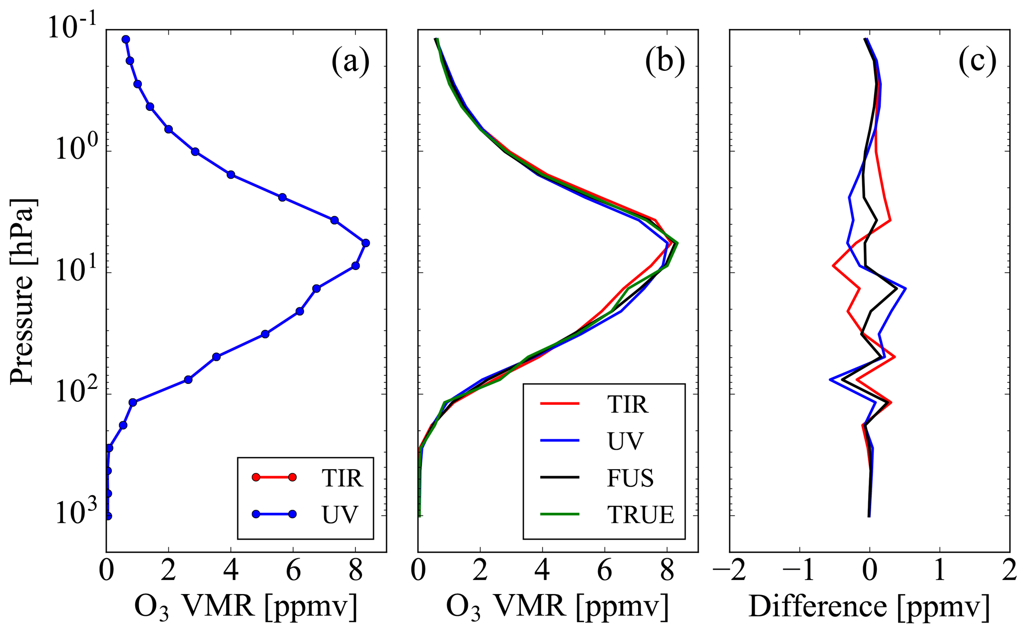
Figure 1 (a) True ozone profiles related to TIR (red line) and UV (blue line) measurements. (b) Ozone profiles obtained from TIR measurement (red line), from UV measurement (blue line), from the data fusion (black line) compared with the mean value of the true profiles (green line). (c) Residual errors obtained as differences of the ozone profiles obtained from TIR measurement (red line), from UV measurement (blue line) and from data fusion (black line) from the mean value of true profiles. All the reported quantities are related to case 1.

Figure 2 As Fig. 1 but for case 2.

Figure 3 As Fig. 1 but for case 3.

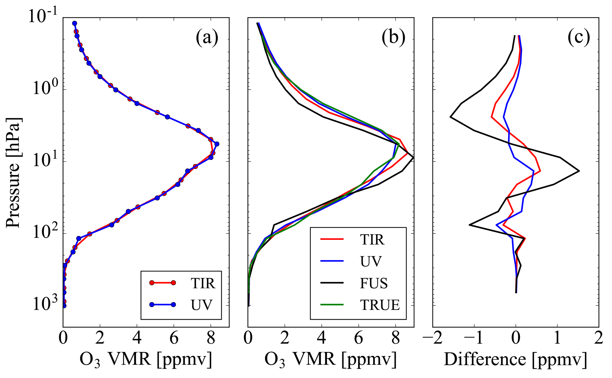
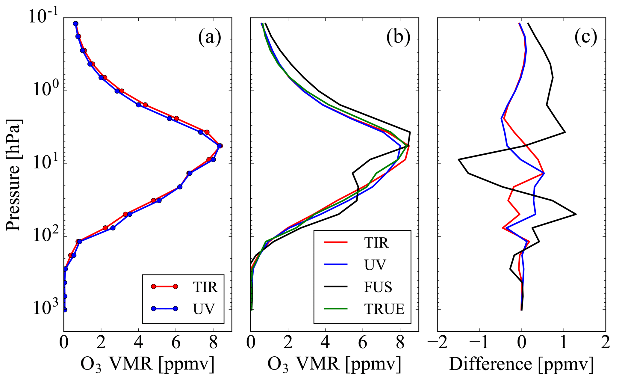
The problem encountered in case 2 is due to the fact that the data fusion is made using estimates of the AKMs on the fusion grid (see Sect. 3.1) obtained by interpolation of the original AKMs (Ceccherini et al., 2016), which are only an approximation of the real AKMs on the fusion grid. We refer to this effect as interpolation error. The problem encountered in case 3 is related to different true profiles and we refer to this effect as coincidence error because it occurs when fusing profiles that do not correspond to the same space–time location.

3 Method

In this section, a theoretical analysis is performed to overcome the problems highlighted in the previous section. In Sect. 3.1, we recall the formulas of the CDF method in order to establish the formalism subsequently used in Sect. 3.2, where an upgrade of the method is proposed.

3.1 CDF

Let us assume to have N independent and simultaneous measurements of the vertical profile of an atmospheric target referred to the same space–time location. Performing the retrieval of the N measurements with the optimal estimation method (Rodgers, 2000), we obtain N vectors ${\widehat{\mathit{x}}}_i$ (i = 1, 2, ... , N) here assumed to be estimates of the profiles made on a common vertical grid. The use of a priori information ensures the possibility of having a common retrieval grid also in the case of observations with different vertical coverage.

The vectors ${\widehat{\mathit{x}}}_i$ are characterized by the CMs S_i and the AKMs A_i (Ceccherini et al., 2003; Ceccherini and Ridolfi, 2010; Rodgers, 2000):

$$\begin{array}{ll}{\displaystyle }& {\displaystyle }{\mathbf{S}}_i\equiv 〈{\mathit{\sigma }}_i{\mathit{\sigma }}_i^T〉={\left({\mathbf{K}}_i^T{\mathbf{S}}_{yi}^{-\mathrm{1}}{\mathbf{K}}_i+{\mathbf{S}}_{ai}^{-\mathrm{1}}\right)}^{-\mathrm{1}}{\mathbf{K}}_i^T{\mathbf{S}}_{yi}^{-\mathrm{1}}{\mathbf{K}}_i\\ \text{(1)}& {\displaystyle }& {\displaystyle }{\left({\mathbf{K}}_i^T{\mathbf{S}}_{yi}^{-\mathrm{1}}{\mathbf{K}}_i+{\mathbf{S}}_{ai}^{-\mathrm{1}}\right)}^{-\mathrm{1}},\text{(2)}& {\displaystyle }& {\displaystyle }{\mathbf{A}}_i\equiv {\displaystyle \frac{\partial {\widehat{\mathit{x}}}_i}{\partial \mathit{x}}}={\left({\mathbf{K}}_i^T{\mathbf{S}}_{yi}^{-\mathrm{1}}{\mathbf{K}}_i+{\mathbf{S}}_{ai}^{-\mathrm{1}}\right)}^{-\mathrm{1}}{\mathbf{K}}_i^T{\mathbf{S}}_{yi}^{-\mathrm{1}}{\mathbf{K}}_i,\end{array}$$

where σ_i are the errors on ${\widehat{\mathit{x}}}_i$ obtained by propagating the errors of the observations through the retrieval processes (noise errors), K_i are the Jacobians of the forward models, S_yi are the CMs of the observations, S_ai are the CMs of the a priori profiles and x is the true profile.

The CDF solution for the considered profiles is given by (see Ceccherini et al., 2015)

$$\begin{array}{ll}{\displaystyle }{\mathit{x}}_{\mathrm{f}}=& {\displaystyle }{\left(\sum _{i=\mathrm{1}}^N{\mathbf{A}}_i^T{\mathbf{S}}_i^{-\mathrm{1}}{\mathbf{A}}_i+{\mathbf{S}}_a^{-\mathrm{1}}\right)}^{-\mathrm{1}}\\ \text{(3)}& {\displaystyle }& {\displaystyle }\left(\sum _{i=\mathrm{1}}^N{\mathbf{A}}_i^T{\mathbf{S}}_i^{-\mathrm{1}}{\mathit{\alpha }}_i+{\mathbf{S}}_a^{-\mathrm{1}}{\mathit{x}}_a\right),\end{array}$$

where

$$\begin{array}{}\text{(4)}& {\displaystyle }{\mathit{\alpha }}_i\equiv {\widehat{\mathit{x}}}_i-\left(\mathbf{I}-{\mathbf{A}}_i\right){\mathit{x}}_{ai}={\mathbf{A}}_i\mathit{x}+{\mathit{\sigma }}_i,\end{array}$$

x_ai is the a priori profile used in the ith retrieval and x_a and S_a are the a priori profile and its CM used to constrain the data fusion.

We note that the vector α_i, which can be calculated from the available retrieval products, is a measurement of the vector x, made using the rows of the AKM A_i, and no longer depends on the a priori profile x_ai. Furthermore, it has the same errors σ_i as the retrieved profile ${\widehat{\mathit{x}}}_i$; therefore, it is characterized by the CM S_i.

The fused profile has a CM, obtained by propagating the errors of α_i into x_f, equal to

$$\begin{array}{ll}{\displaystyle }{\mathbf{S}}_{\mathrm{f}}=& {\displaystyle }{\left(\sum _{i=\mathrm{1}}^N{\mathbf{A}}_i^T{\mathbf{S}}_i^{-\mathrm{1}}{\mathbf{A}}_i+{\mathbf{S}}_a^{-\mathrm{1}}\right)}^{-\mathrm{1}}\sum _{i=\mathrm{1}}^N{\mathbf{A}}_i^T{\mathbf{S}}_i^{-\mathrm{1}}{\mathbf{A}}_i\\ \text{(5)}& {\displaystyle }& {\displaystyle }{\left(\sum _{i=\mathrm{1}}^N{\mathbf{A}}_i^T{\mathbf{S}}_i^{-\mathrm{1}}{\mathbf{A}}_i+{\mathbf{S}}_a^{-\mathrm{1}}\right)}^{-\mathrm{1}}\end{array}$$

and an AKM, obtained performing the derivative of x_f with respect to the true profile, equal to

$$\begin{array}{}\text{(6)}& {\displaystyle }{\mathbf{A}}_{\mathrm{f}}={\left(\sum _{i=\mathrm{1}}^N{\mathbf{A}}_i^T{\mathbf{S}}_i^{-\mathrm{1}}{\mathbf{A}}_i+{\mathbf{S}}_a^{-\mathrm{1}}\right)}^{-\mathrm{1}}\sum _{i=\mathrm{1}}^N{\mathbf{A}}_i^T{\mathbf{S}}_i^{-\mathrm{1}}{\mathbf{A}}_i.\end{array}$$

The CDF formula (Eq. 3) involves a summation of AKMs made possible by the common grid. When the fusing profiles ${\widehat{\mathit{x}}}_i$ are represented on different vertical grids, the available AKMs are also defined on different vertical grids; thus in this case, it is necessary to perform a resampling of the AKMs (Calisesi et al., 2005), which makes their second index equal to that of the common fusion grid. Following Ceccherini et al. (2016), we define such a transformation as follows:

$$\begin{array}{}\text{(7)}& {\displaystyle }{\mathbf{A}}_i^{\prime }={\mathbf{A}}_i{\mathbf{R}}_i,\end{array}$$

where R_i are the generalized inverse matrices of the linear interpolation matrices H_i, which interpolate the profiles on the fusing grids to the fusion grid. In this case, using Eq. (7), Eq. (3) becomes

$$\begin{array}{ll}{\displaystyle }{\mathit{x}}_{\mathrm{f}}=& {\displaystyle }{\left(\sum _{i=\mathrm{1}}^N{\mathbf{R}}_i^T{\mathbf{A}}_i^T{\mathbf{S}}_i^{-\mathrm{1}}{\mathbf{A}}_i{\mathbf{R}}_i+{\mathbf{S}}_a^{-\mathrm{1}}\right)}^{-\mathrm{1}}\\ \text{(8)}& {\displaystyle }& {\displaystyle }\left(\sum _{i=\mathrm{1}}^N{\mathbf{R}}_i^T{\mathbf{A}}_i^T{\mathbf{S}}_i^{-\mathrm{1}}{\mathit{\alpha }}_i+{\mathbf{S}}_a^{-\mathrm{1}}{\mathit{x}}_a\right).\end{array}$$

We notice that, in the case of different vertical grids, only the AKMs must be interpolated; neither the CMs nor the α_i vectors need to be interpolated.

3.2 Interpolation and coincidence errors

Let us first consider the interpolation error. The vectors α_i, defined by Eq. (4), are measurements of the true profile, each made with the averaging kernels A_i. Let us assume that each measurement is defined on a different retrieval grid, identified by the same index that identifies the measurements; thus, Eq. (4) becomes

$$\begin{array}{}\text{(9)}& {\displaystyle }{\mathit{\alpha }}_i={\mathbf{A}}_i{\mathit{x}}_i^{\left(i\right)}+{\mathit{\sigma }}_i,\end{array}$$

where ${\mathit{x}}_i^{\left(i\right)}$ is the true profile related to the ith measurement that, by definition, is sampled with the ith grid, as highlighted by the superscript in parentheses.

Equation (8) shows that in the presence of different vertical grids the CDF method combines measurements with sensitivity to the true profile expressed by A_iR_i. This operation assumes that the measurements are combined on the common fusion grid, i.e. measurements of A_iR_i${\mathit{x}}_i^{\left(f\right)}$, with ${\mathit{x}}_i^{\left(f\right)}$ being the true profile related to the ith measurement represented on the fusion grid. If using α_i (Eq. 9), which is the measurement of ${\mathbf{A}}_i{\mathit{x}}_i^{\left(i\right)}$, the estimate of the required measurement A_iR_i${\mathit{x}}_i^{\left(f\right)}$ is made with an error equal to ${\mathbf{A}}_i{\mathit{x}}_i^{\left(i\right)}-{\mathbf{A}}_i{\mathbf{R}}_i{\mathit{x}}_i^{\left(f\right)}$.

We can explicitly introduce this error in the expression of α_i by rearranging Eq. (9) in the following way:

$$\begin{array}{}\text{(10)}& {\displaystyle }{\mathit{\alpha }}_i={\mathbf{A}}_i{\mathbf{R}}_i{\mathit{x}}_i^{\left(f\right)}+{\mathbf{A}}_i\left({\mathit{x}}_i^{\left(i\right)}-{\mathbf{R}}_i{\mathit{x}}_i^{\left(f\right)}\right)+{\mathit{\sigma }}_i.\end{array}$$

It is useful to introduce the following notations for ${\mathit{x}}_i^{\left(i\right)}$ and ${\mathit{x}}_i^{\left(f\right)}$:

$$\begin{array}{}\text{(11)}& {\displaystyle }& {\displaystyle }{\mathit{x}}_i^{\left(i\right)}={\mathbf{C}}^{\left(i\right)}{\mathit{x}}_i,\text{(12)}& {\displaystyle }& {\displaystyle }{\mathit{x}}_i^{\left(f\right)}={\mathbf{C}}^{\left(f\right)}{\mathit{x}}_i,\end{array}$$

where x_i is the true profile related to the ith measurement represented on a very fine grid that includes all the levels of the fusion grid (f) and of the N grids (i). C⁽ⁱ⁾ and C^(f)are the sampling matrices from the fine grid to the grids (i) and to the grid (f), respectively.

Substituting Eqs. (11) and (12) in Eq. (10), one obtains

$$\begin{array}{}\text{(13)}& {\displaystyle }{\mathit{\alpha }}_i={\mathbf{A}}_i{\mathbf{R}}_i{\mathbf{C}}^{\left(f\right)}{\mathit{x}}_i+{\mathbf{A}}_i\left({\mathbf{C}}^{\left(i\right)}-{\mathbf{R}}_i{\mathbf{C}}^{\left(f\right)}\right){\mathit{x}}_i+{\mathit{\sigma }}_i.\end{array}$$

Let us now also consider the coincidence error. In general, measurements made in different space–time locations are only fused when they lie within a given coincidence criterion. These measurements correspond to different true profiles and the purpose of the data fusion can be the determination of either the mean value of these true profiles or the true profile in a given space–time location identified as the central point of the coincidence intervals. We indicate with $\stackrel{\mathrm{‾}}{\mathit{x}}$ the unknown profile estimated by the data fusion. If we introduce the quantity σ_i,coin, which gives the deviation of x_i from the unknown profile $\stackrel{\mathrm{‾}}{\mathit{x}}$,

$$\begin{array}{}\text{(14)}& {\displaystyle }{\mathit{x}}_i=\stackrel{\mathrm{‾}}{\mathit{x}}+{\mathit{\sigma }}_{i,\mathrm{coin}},\end{array}$$

then Equation (13) becomes

$$\begin{array}{ll}{\displaystyle }& {\displaystyle }{\mathit{\alpha }}_i={\mathbf{A}}_i{\mathbf{R}}_i{\mathbf{C}}^{\left(f\right)}\stackrel{\mathrm{‾}}{\mathit{x}}+{\mathbf{A}}_i\left({\mathbf{C}}^{\left(i\right)}-{\mathbf{R}}_i{\mathbf{C}}^{\left(f\right)}\right)\stackrel{\mathrm{‾}}{\mathit{x}}+{\mathbf{A}}_i{\mathbf{C}}^{\left(i\right)}{\mathit{\sigma }}_{i,\mathrm{coin}}\\ {\displaystyle }& {\displaystyle }+{\mathit{\sigma }}_i={\mathbf{A}}_i{\mathbf{R}}_i{\stackrel{\mathrm{‾}}{\mathit{x}}}^{\left(f\right)}+{\mathbf{A}}_i\left({\mathbf{C}}^{\left(i\right)}-{\mathbf{R}}_i{\mathbf{C}}^{\left(f\right)}\right)\stackrel{\mathrm{‾}}{\mathit{x}}\\ \text{(15)}& {\displaystyle }& {\displaystyle }+{\mathbf{A}}_i{\mathbf{C}}^{\left(i\right)}{\mathit{\sigma }}_{i,\mathrm{coin}}+{\mathit{\sigma }}_i\end{array}$$

after using Eq. (12) for $\stackrel{\mathrm{‾}}{\mathit{x}}$.

An estimate of the quantity ${\mathbf{A}}_i\left({\mathbf{C}}^{\left(i\right)}-{\mathbf{R}}_i{\mathbf{C}}^{\left(f\right)}\right)\stackrel{\mathrm{‾}}{\mathit{x}}$ can be obtained writing $\stackrel{\mathrm{‾}}{\mathit{x}}$ as the a priori profile plus the deviation σ_a from it:

$$\begin{array}{}\text{(16)}& {\displaystyle }\stackrel{\mathrm{‾}}{\mathit{x}}={\mathit{x}}_a+{\mathit{\sigma }}_a.\end{array}$$

Substituting Eq. (16) in Eq. (15) and rearranging the terms of the equation, we can define a new quantity, ${\stackrel{\mathrm{̃}}{\mathit{\alpha }}}_i$, equal to

$$\begin{array}{ll}{\displaystyle }{\stackrel{\mathrm{̃}}{\mathit{\alpha }}}_i& {\displaystyle }\equiv {\mathit{\alpha }}_i-{\mathbf{A}}_i\left({\mathbf{C}}^{\left(i\right)}-{\mathbf{R}}_i{\mathbf{C}}^{\left(f\right)}\right){\mathit{x}}_a\\ {\displaystyle }& {\displaystyle }={\mathbf{A}}_i{\mathbf{R}}_i{\stackrel{\mathrm{‾}}{\mathit{x}}}^{\left(f\right)}+{\mathbf{A}}_i\left({\mathbf{C}}^{\left(i\right)}-{\mathbf{R}}_i{\mathbf{C}}^{\left(f\right)}\right){\mathit{\sigma }}_a\\ \text{(17)}& {\displaystyle }& {\displaystyle }+{\mathbf{A}}_i{\mathbf{C}}^{\left(i\right)}{\mathit{\sigma }}_{i,\mathrm{coin}}+{\mathit{\sigma }}_i.\end{array}$$

Each ${\stackrel{\mathrm{̃}}{\mathit{\alpha }}}_i$ is a measurement of ${\stackrel{\mathrm{‾}}{\mathit{x}}}^{\left(f\right)}$ made using the rows of the matrix A_iR_i and a total error given by the sum of the noise error σ_i plus the terms A_i(C⁽ⁱ⁾−R_iC^(f))σ_a and A_iC⁽ⁱ⁾σ_i,coin that can be interpreted as the interpolation error and the coincidence error, respectively.

For the estimate of the interpolation error, we use the a priori CM S_a of σ_a and, therefore, the interpolation error is characterized by the CM:

$$\begin{array}{}\text{(18)}& {\displaystyle }{\mathbf{S}}_{i,\mathrm{int}}={\mathbf{A}}_i\left({\mathbf{C}}^{\left(i\right)}-{\mathbf{R}}_i{\mathbf{C}}^{\left(f\right)}\right){\mathbf{S}}_a{\left({\mathbf{C}}^{\left(i\right)}-{\mathbf{R}}_i{\mathbf{C}}^{\left(f\right)}\right)}^T{\mathbf{A}}_i^T.\end{array}$$

To characterize the coincidence error, we introduce the CM S_coin of σ_i,coin. If $\stackrel{\mathrm{‾}}{\mathit{x}}$ represents the mean value of the true profiles, S_coin accounts for the dispersion of the true profiles, thus it depends on the coincidence criteria and it is the same for all the measurements to be fused together. If $\stackrel{\mathrm{‾}}{\mathit{x}}$ represents the true profile in a specific space–time location, S_coin is zero if the measurement is exactly in that location and it increases going away from that location. The values of S_coin as a function of space–time location should reflect the variability of the true profile with the location. Then, the coincidence error is characterized by the CM

$$\begin{array}{}\text{(19)}& {\displaystyle }{\mathbf{S}}_{i,\mathrm{coin}}={\mathbf{A}}_i{\mathbf{C}}^{\left(i\right)}{\mathbf{S}}_{\mathrm{coin}}{\mathbf{C}}^{\left(i\right)T}{\mathbf{A}}_i^T.\end{array}$$

In conclusion, the CDF formula, given by Eq. (3), can be modified to account for the interpolation and coincidence errors by replacing α_i with

$$\begin{array}{}\text{(20)}& {\displaystyle }{\stackrel{\mathrm{̃}}{\mathit{\alpha }}}_i={\mathit{\alpha }}_i-{\mathbf{A}}_i\left({\mathbf{C}}^{\left(i\right)}-{\mathbf{R}}_i{\mathbf{C}}^{\left(f\right)}\right){\mathit{x}}_a\end{array}$$

and S_i with

$$\begin{array}{}\text{(21)}& {\displaystyle }{\stackrel{\mathrm{̃}}{\mathbf{S}}}_i={\mathbf{S}}_i+{\mathbf{S}}_{i,\mathrm{int}}+{\mathbf{S}}_{i,\mathrm{coin}}.\end{array}$$

The CM given by Eq. (21) is also used in place of S_i in Eqs. (5) and (6) for the calculation of the CM and AKM of the fused profile.

4 Tests with the upgraded algorithm: results and discussion

4.1 The effect on fused profiles

The test cases of fusion 2 and 3 shown in Sect. 2 are here repeated with the modified method described in Sect. 3.2.

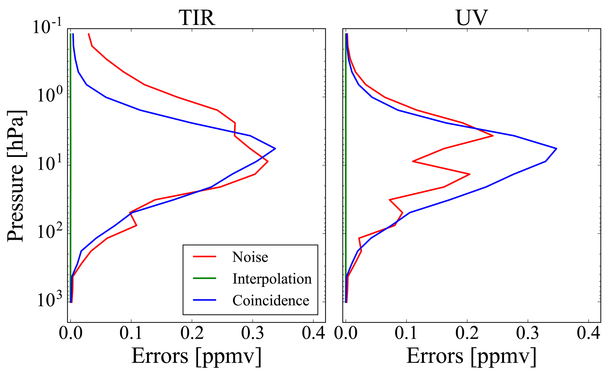
In Figs. 4 and 5, we report the noise errors, the interpolation errors and the coincidence errors related, respectively, to case 2 and case 3, for both TIR and UV measurements. These errors are calculated as the square root of the diagonal elements of S_i, S_i,int and S_i,coin, respectively. In case 2, the vertical grids are different for the two measurements, and since the fusion grid coincides with the vertical grid of the UV measurement, the interpolation errors are different from zero for the TIR measurement and equal to zero for the UV measurement. The coincidence errors are equal to zero in both TIR and UV measurements because the true profiles are the same. In case 3, the interpolation errors are equal to zero for both TIR and UV measurements because the fusion grid coincides with that of the fusing profiles. The coincidence errors are instead different from zero because the true profiles are different and their CMs, chosen equal for both TIR and UV measurements, are obtained considering an error of 5 % of the a priori profile (consistent with the difference between the true profiles) and a correlation length of 6 km.

Figures 6 and 7 show the fused profiles and the residuals obtained with the modified algorithm compared with the same quantities reported in panels (b) and (c) of Figs. 2 and 3, respectively. In both tests, the modified method provides residuals that are significantly smaller than those obtained with the original CDF method.

Figure 4 Noise errors (red lines), interpolation errors (green lines) and coincidence errors (blue lines) in case 2 for TIR and UV measurements.

Figure 5 As Fig. 4 but for case 3.

These tests show that the upgrade of the CDF method proposed in Sect. 3.2 solves the problems observed in Sect. 2 that occur when either the fusing profiles are retrieved on different vertical grids or they refer to different true profiles. The modified method is a generalization of the CDF that allows its application to a wide range of cases.

Figure 6 The fused profile and the residual error obtained with the modified algorithm (magenta lines) compared with the same quantities of Fig. 2b and c.

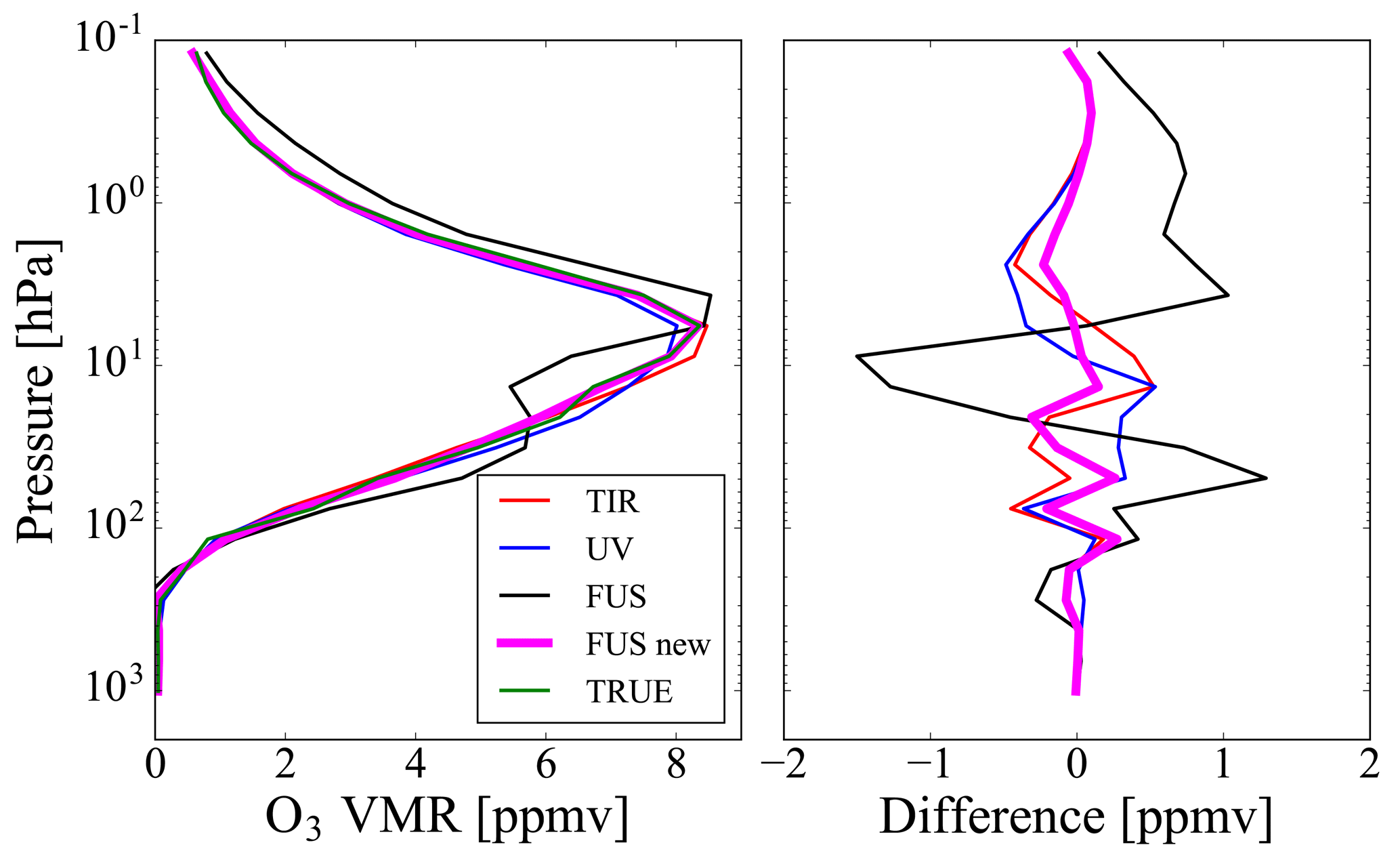
Figure 7 The fused profile and the residual error obtained with the modified algorithm (magenta lines) compared with the same quantities of Fig. 3b and c.

4.2 The effect on errors and number of DOF

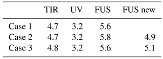
We now look at the effect of the generalized method on the errors and on the number of DOF. Figures 8 and 9 show the errors of the fused profile when we use either the original or the modified method for cases 2 and 3, respectively. These errors are calculated as the square root of the diagonal elements of S_f given in Eq. (5), where, in the modified method, S_i is replaced by ${\stackrel{\mathrm{̃}}{\mathbf{S}}}_i$. For the three cases described in Sect. 2, Table 1 gives the number of DOF of the profiles obtained from the individual TIR and UV measurements, and from the CDF method using both the original and the generalized formulation. The numbers of DOF are calculated as the trace of the AKMs. For the fused products the AKM is A_f given by Eq. (6), where, in the generalized formulation, S_i is replaced by ${\stackrel{\mathrm{̃}}{\mathbf{S}}}_i$.

The introduction of the interpolation error (case 2) does not significantly modify the errors and determines a decrease in the number of DOF of the fused profile of about 1. The introduction of the coincidence error (case 3) determines a significant increase in the errors and a small decrease in the number of DOF of the fused profile equal to about 0.5. However, in both cases the number of DOF of the fused profile obtained with the modified method is larger than the number of DOF of the individual fusing profiles, proving the information gain provided by the fusion.

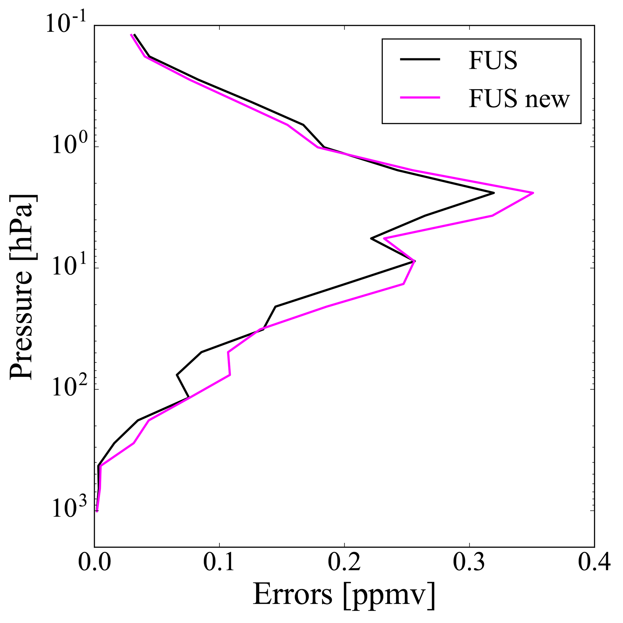
Figure 8 Errors of the fused profile when we use the original (black line) and the generalized (magenta line) CDF for case 2.

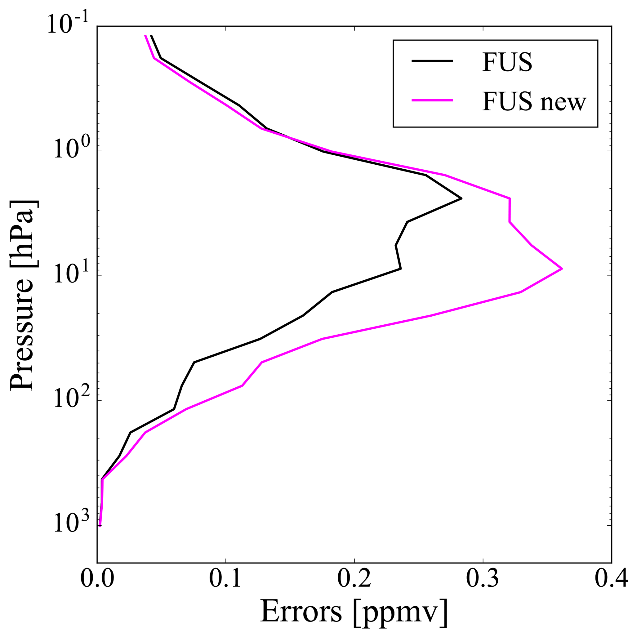
Figure 9 Errors of the fused profile when we use the original (black line) and the generalized (magenta line) CDF for case 3.

From the analysis of errors and number of DOF we deduce that the interpolation error has the largest impact on the vertical resolution, while the coincidence error has the largest impact on the errors. However, these numerical results depend on the values that interpolation and coincidence errors have in the single cases.

Table 1 Number of DOF of the profiles obtained with the TIR measurement, the UV measurement, the original fusion method and the modified fusion method for each of the three cases described in Sect. 2.

5 Other error sources

In this paper, we considered simulated measurements, which generally do not include all the error components that are present in real measurements. When real measurements are considered, there are other important error sources that can cause inconsistency among the fusing profiles, such as forward model errors, due, for example, to approximations in the model and uncertainties in atmospheric and instrumental parameters. When performing data fusion, these errors can also lead to quality loss and show problems similar to those described in Sect. 2. These problems can be avoided by accounting for them in the CDF formulation. In particular, Eq. (21) can be modified to account for an extra CM term, S_i,other, as follows:

$$\begin{array}{}\text{(22)}& {\displaystyle }{\stackrel{\mathrm{̃}}{\mathbf{S}}}_i={\mathbf{S}}_i+{\mathbf{S}}_{i,\mathrm{other}}+{\mathbf{S}}_{i,\mathrm{int}}+{\mathbf{S}}_{i,\mathrm{coin}}.\end{array}$$

6 Conclusions

We analysed the problem posed by the application of the CDF method to vertical profiles obtained with different instruments, which use different retrieval grids and observe different true profiles. To this purpose, we studied simulated ozone profile measurements expected from the MTG payload for the S4 mission of the Copernicus programme: namely, those provided by the IRS in the thermal infrared and by the UVN spectrometer in the ultraviolet. The study showed that the CDF algorithm works well when the fusing profiles are represented on the same vertical grid and refer to the same true profile; otherwise the algorithm provides unsatisfactory results because the fused profile differs from the mean of the true profiles significantly more than the fusing profiles. In the latter case, the CDF method, which uses all the existing information for the determination of the best fused profile, is exploiting the differences due to the inconsistency of the measurements as useful information and provides unrealistic fused profiles.

In order to overcome this new problem, we performed a theoretical analysis that led to a generalization of the CDF method to the cases in which interpolation and coincidence errors occur. The interpolation error is present when the vertical grids of the fusing profiles differ from the fusion grid, meaning that an interpolation of the AKMs is necessary. In this case, the interpolated AKMs are only an approximation of the real AKMs on the fusion grid. The coincidence error is a consequence of the fact that the fusing profiles are not generally co-located in space and time, thus referring to different true profiles.

The generalized algorithm allows for these inconsistencies and provides fused profiles that are in better agreement with the true profiles than those obtained with the original CDF algorithm.

With the new algorithm, the fusion generally provides fused profiles that are also better than the fusing profiles in terms of total error and number of DOF. However, a more comprehensive error budget, which may even cause the fused profile to have larger errors than the fusing profiles (coincidence and interpolation errors do not have to be considered for the individual fusing profiles), is now considered. If neither of the qualifiers (total error and number of DOF) is improved, the fusion process is not justified.

An approach similar to that used to account for interpolation and coincidence errors can also be useful to include other error components, such as forward model errors, in the fusion process.