the Creative Commons Attribution 4.0 License.
the Creative Commons Attribution 4.0 License.
 | 28 Feb 2018
Information content analysis: the potential for methane isotopologue retrieval from GOSAT-2
Yukio Yoshida
Tsuneo Matsunaga
Jan-Peter Muller
Atmospheric methane is comprised of multiple isotopic molecules, with the most abundant being 12CH4 and 13CH4, making up 98 and 1.1 % of atmospheric methane respectively. It has been shown that is it possible to distinguish between sources of methane (biogenic methane, e.g. marshland, or abiogenic methane, e.g. fracking) via a ratio of these main methane isotopologues, otherwise known as the δ13C value. δ13C values typically range between −10 and −80 ‰, with abiogenic sources closer to zero and biogenic sources showing more negative values. Initially, we suggest that a δ13C difference of 10 ‰ is sufficient, in order to differentiate between methane source types, based on this we derive that a precision of 0.2 ppbv on 13CH4 retrievals may achieve the target δ13C variance. Using an application of the well-established information content analysis (ICA) technique for assumed clear-sky conditions, this paper shows that using a combination of the shortwave infrared (SWIR) bands on the planned Greenhouse gases Observing SATellite (GOSAT-2) mission, 13CH4 can be measured with sufficient information content to a precision of between 0.7 and 1.2 ppbv from a single sounding (assuming a total column average value of 19.14 ppbv), which can then be reduced to the target precision through spatial and temporal averaging techniques. We therefore suggest that GOSAT-2 can be used to differentiate between methane source types. We find that large unconstrained covariance matrices are required in order to achieve sufficient information content, while the solar zenith angle has limited impact on the information content.
- Article
(16283 KB) - Full-text XML
- BibTeX
- EndNote


Of the major greenhouse gases (GHGs) currently considered to have a major impact on atmospheric chemistry, methane is amongst the most important. The potential for atmospheric heating by methane is well documented (IPCC, 2014; Khalil and Rasmussen, 1994; Kirschke et al., 2013; Wuebbles and Hayhoe, 2002). Excess concentrations of atmospheric methane can lead to detrimental effects on the chemistry of the atmosphere and to the absorption of infrared (IR) radiation causing atmospheric heating. Methane concentration in the atmosphere has been documented to be rising steadily over the past century, aside from a short period in the middle of the last decade (Heimann, 2011; Kai et al., 2011), leading to renewed efforts to understand global atmospheric methane. In order to tackle the problem of growing methane concentrations, it is necessary to understand the nature of the global sources of methane that will allow for a greater understanding of the processes behind methane generation and how they will affect the global environment. A key point is that the global methane budget is still not truly understood; this is highlighted by the “pause” in the increase in global methane concentration in the last decade, for which there are many contrasting arguments published explaining its cause (Aydin et al., 2011; Heimann, 2011; Kai et al., 2011). Towards this end of understanding global methane emissions (and other GHGs), multiple satellite missions have been launched, including the SCanning Imaging Absorption spectroMeter for Atmospheric CHartographY (SCIAMACHY) (Bovensmann et al., 1999) and the Greenhouse gases Observing SATellite (GOSAT) (Kuze et al., 2009), with future GHG monitoring missions currently under development.
What is suggested is that there may be profound disagreement as to whether the majority of atmospheric methane occurs from natural or anthropogenic sources, and satellite measurements to date have not yet addressed this problem. Towards this end, we consider an assessment of the potential of measuring the main isotopologues of methane (methane consisting of different carbon and/or hydrogen isotopes) from a spaceborne instrument. Atmospheric methane is primarily composed of two key isotopologues, 12CH4 and 13CH4, which have a natural abundance of about 98 and 1.1 % respectively. It is a well-established fact that different sources of methane (i.e. biogenic sources such as methanogens and Arctic permafrost or non-biogenic such as industrial hydrocarbon burning) vary in the abundance of these isotopologues (Etiope, 2009; Rigby et al., 2012). This fractionation between sources generally occurs for two reasons. (1) Plant-based photosynthesis enzymes discriminate against 13C carbon dioxide (13CO2) during uptake because of the higher isotopic mass, and thus most plant-based material is depleted in 13C hydrocarbons. (2) The bacterial reduction of carbon dioxide to methane is associated with a kinetic isotope effect, which discriminates against 13C, thus leaving depleted 13CH4 concentrations in biogenic methane sources (Levin et al., 1993; Whiticar, 1999). This nominally occurs in soil and therefore is not associated with the other forms of methane (thermogenic and abiogenic). Comprehensive reviews of these discriminations and global sources of such are reviewed in more detail elsewhere (Nisbet et al., 2016; Schaefer et al., 2016; Schwietzke et al., 2016).
Methane isotopologue measurements of a sample of air are typically expressed as per mil ratios of the heavier to lighter isotopologues relative to an established literature standard, which in the case of 13C to 12C is Vienna Pee Dee Belemnite (VPDB; Craig, 1957). This ratio is known as the δ13C value and is common in established literature relating to methane isotopologues. However, normally such values are used in reference to in situ samples within the troposphere. In the case of this work, we assume all measurements are in the form of total column-averaged values, which will have some differences associated with them in comparison to in situ tropospheric measurements. Note that VPDB is unusually enriched in 13C methane, meaning that all measurements taken in reference to VPDB will most likely have negative values. Due to the reasons stated above, biogenic sources of methane will have δ13C values in the range of −60 to −80 ‰, while industrial sources should have values closer to −40 or −30 ‰ (Rigby et al., 2012).
Unlike methane, global measurements of the δ13C ratio are much more limited, with most of the publically available data restricted to 20 sites of in situ measurements from the National Oceanic and Atmospheric Administration (NOAA) Carbon Cycle Greenhouse Gas cooperative air sampling network (http://www.esrl.noaa.gov/gmd/ccgg/flask.html). Although these measurements are extremely accurate and useful in their own right, they are limited by their sparseness and physical location. They are all in areas which sample background values rather than anomalies associated with large methane sources. This means that they can only provide limited guidance on global distributions of δ13C. Some measurements from balloon soundings (Röckmann et al., 2011) and satellite-based solar occultation measurements (Buzan et al., 2016) are available, but these only sample the atmosphere from the middle to the upper troposphere, where methane is well mixed. In the troposphere Hydroxyl acts as the main methane sink and is likely to destroy the original isotopologue signature and so miss the key activity which occurs in the lower troposphere and is of most interest to the scientific community. Such lower-tropospheric activity can only be captured from a satellite instrument with a nadir sounding profile, preferably in the shortwave infrared (SWIR). Therefore, if total column soundings of δ13C can be retrieved from a satellite platform and yield enough information with a sufficiently high degree of precision, there is potential for very useful information on the global distribution of biogenic and non-biogenic methane sources.
The fact that we are mostly interested in lower-tropospheric sources of methane makes satellite measurements in the SWIR band much more useful than in the thermal infrared (TIR) due to higher surface sensitivity (Herbin et al., 2013; Worden et al., 2007). Most current and future SWIR nadir satellites assume a passive solar–surface–satellite light path, which is largely the cause of higher surface sensitivity for these instruments. This statement is built on the assumption of a significant number of methane isotopologues spectral lines present in the SWIR and in the sensitivity ranges of any instruments. However, this particular passive remote sensing method is highly susceptible to light path modification due to aerosols and clouds, thus adding high degrees of uncertainty to the retrieval. Because in this assessment we are interested in the ratio of two gases (12CH4 and 13CH4), we can apply the proxy method (Frankenberg et al., 2011; Parker et al., 2011), which assumes that the light path modification of two spectrally close traces gases will be similar and will, therefore, cancel out when calculating a ratio. The High-Resolution Transmission (HITRAN) 2012 database (Rothman et al., 2013) states that there are multiple methane isotopologues absorption features present in the 1600–1700 and 2200–2300 nm wavebands. Both of these wavebands are included in the sensitivity range of the planned GOSAT-2/TANSO-FTS-2 instrument (GOSAT-2 Project Team, 2017). Therefore, in order to maximise the potential quantity of information available to a given instrument, this work focuses on the degree of information available in the GOSAT-2 sensitivity range. Although the primary goal of this work is to investigate GOSAT-2, the 1600–1700 nm waveband is also present in the current GOSAT/TANSO-FTS instrument, and therefore any investigations into this waveband with GOSAT-2 are also likely to be applicable to GOSAT.
In this work, we apply the well-established information content analysis (ICA) techniques originally proposed by Rodgers (2000) to determine the potential benefit of retrieving total column methane isotopologue concentrations using bands 2 and 3 of the GOSAT-2/TANSO-FTS-2 instrument. The value of such studies has been proven on multiple occasions (Frankenberg et al., 2012; Herbin et al., 2013; Kuai et al., 2010; Yoshida et al., 2011), providing guidance on appropriate potential retrieval set-ups in order to maximise information received from trace gas retrievals. The original optimal estimation method (OEM) proposed by Rodgers (2000) generally requires a priori knowledge of the retrieval set-up. However, due to the fact that there has been limited research in this area and no a priori state vectors or variance covariance matrices (VCMs) have been defined previously, we test a number of VCMs in order to explore the constraints on retrieving independent information in the total column based on the ICA. This analysis and VCM variations also provide an opportunity to explore the potential errors associated with retrievals of isotopologues in these wavebands (Ceccherini and Ridolfi, 2010; Yoshida et al., 2011).
In the following subsection, we describe the requirements for detecting methane isotopologues as well as the tools and assumed instruments employed during the course of this research.
2.1 Precision requirements for retrieval
Analysis of global δ13C concentrations by Nisbet et al. (2016) shows that trends and variations in δ13C on a regional scale are of the order of a few per mil, which suggests that any total column retrieval algorithm will have to obtain better than this precision in order to comment on trends in δ13C. Given the above assessment, a much more likely prospect is the analysis of localised regions. Nisbet et al. (2016) state that they can see wider ranges in the δ13C of different source regions: for example, Arctic and boreal wetland regions show a per mil value of −70, while Siberian gas fields are at the −50 mark.
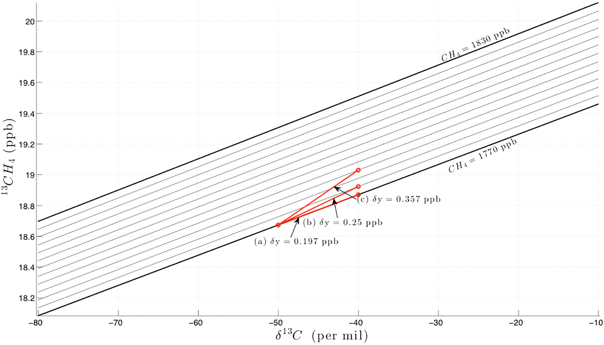
Figure 1Range of expected terrestrial 13CH4 values (y axis) given a range of CH4 values between 1770 and 1830 ppbv, and δ13C between −80 and −10 ‰ (x axis). The diagonal solid lines represent the 12CH4 values for a given CH4 value, while varying the δ13C range. There are 13 12CH4 lines representing the CH4 range in 5 ppbv steps. The red line (a) shows the 13CH4 change between −50 and −40 δ13C for a CH4 of 1770 ppb; line (b) is as line (a) but includes a CH4 change of 5 ppbv; line (c) is as lines (a) and (b) but includes a CH4 change of 15 ppbv.
The δ13C ratio is calculated as follows:
where “sample” refers to the current measurement and “standard” refers to the VPDB value. Rigby et al. (2012) suggest that there is a minimum margin of 10 ‰ in terms of differentiating between fossil fuel and biogenic sources. Using this margin as a base, and applying Eq. (1), we can estimate the minimum precision on 13C methane measurements required to achieve this per mil margin. Firstly we perform a trivial rearrangement of Eq. (1) to make the sample 13CH4 as the subject of the equation. We then specify two ranges of values in order to calculate the range of 13CH4 values that will likely be encountered terrestrially: (1) δ13C range from −80 to −10 ‰, in 10 ‰ steps; (2) 12CH4 range calculated from a CH4 range of 1770–1830 ppbv in 5 ppbv steps, where 12CH4 is assumed to have been calculated from the HITRAN 12CH4 abundance ratio (0.988274; see http://hitran.iao.ru/molecule/simlaunch?mol=6). Using these ranges, we can represent an expected range of terrestrial 13CH4 abundances using Eq. (1).
Taking line (a) in Fig. 1, we show that a change in 13CH4 of ∼ 0.2 ppbv is observed for a 10 ‰ δ13C shift; this initially implies that a precision of 0.2 ppbv on 13CH4 retrievals is required to resolve δ13C measurements to a 10 ‰ resolution. However, we have to take into account the precision on total column methane measurements from GOSAT, which Yoshida et al. (2011) state to be 6 ppbv on average and roughly 15 ppbv at minimum (with Parker et al., 2015, also showing a minimum precision of roughly 15 ppbv). Taking these precisions into account, lines (b) and (c) in Fig. 1 show that there is an additional 0.053 ppbv uncertainty on 13CH4 concentration for 5 ppbv uncertainty on CH4 (multiplied by 0.988274 to get 12CH4) concentration and a 0.16 ppbv uncertainty on 13CH4 concentration for 15 ppbv uncertainty on CH4 concentration. Using Eq. (1) we can determine that a 0.053 ppbv 13CH4 uncertainty equates to a δ13C uncertainty of 2.7 ‰, and a 0.16 ppbv 13CH4 uncertainty equates to a δ13C uncertainty of 8 ‰. Therefore the goal of this research is to establish whether GOSAT-2 can reach a target 13CH4 precision of 0.2 ppbv, equating to a δ13C precision of 10 ‰, with the caveat that on average there will be a 2.7 ‰ uncertainty associated with this value and a maximum uncertainty of 8 ‰. For the average methane precision, source differentiation should still be possible; however, when considering the lowest precision methane, it is likely that we lose the ability to differentiate between source types for certain, but it may still be possible if the measured δ13C values were at the extreme end of the scale. Because of this, we will set additional 13CH4 precision goals of 0.147 and 0.04 ppbv in order to achieve the eventual desired δ13C precision of 10 ‰.
Note that Fig. 1 shows a linear relationship between δ13C quantities and between CH4 quantities; therefore although the above assessment focused on the 10 ‰ range between −50 and −40, the assessment applies to any ranges on the figure.
In addition to measurement precision errors, numerous studies have suggested that a bias of ∼ 5 ppbv can be expected on methane retrievals in GOSAT (Parker et al., 2015; Schepers et al., 2012; Yoshida et al., 2013). These biases are caused by numerous effects (e.g. errors in the forward models) and are explored in more detail in the previously mentioned papers. The calculations above suggest that for a bias of 5 ppbv, a δ13C bias of 2.7 ‰ can be expected. However, we expect additional biases to appear on 13CH4 retrievals, in addition to those on 12CH4 retrievals. These are difficult to quantify exactly because the previously reported biases of CH4 from GOSAT are based on comparisons with the Total Column Carbon Observing Network (TCCON; Wunch et al., 2011). No such measurements exist for 13CH4 currently and so we cannot estimate these biases.
2.2 The Oxford Reference Forward Model (ORFM)
The ORFM (Dudhia, 2017) is a general line-by-line (GENLN2) based radiative transfer model (RTM) originally developed at the University of Oxford to provide reference spectral calculations for the Michelson Interferometer for Passive Atmospheric Sounding (MIPAS) instrument based on the ENVISAT satellite. The MIPAS instrument was a limb-viewing instrument, and as such the ORFM originally could only handle limb-based calculations. However, in the intervening years the ORFM has been updated significantly in order to be applicable to nadir-viewing instruments. In accordance with these updates multiple viewing geometries are possible (allowing for multiple instrument viewing types such as balloons, aircraft or satellites), 1-D and 2-D atmospheres can be leveraged depending on the application of the user, and surface elevation can be modelled either through modifying a model atmosphere or through setting the height of a ground-based observer. Surface effects can be modelled through modification of surface temperature and emissivity in the case of TIR and of SWIR through a specular reflectance model in the case. However, for surface reflectance we deemed that specular reflectance was not sufficient to accurately model surface scattering. We therefore replaced this specular model with a Lambertian reflectance model (on the assumption that Lambertian reflectance accurately represents ground surface reflectance; Yoshida et al., 2011). The ORFM allows for the modelling of advanced spectral effects such as water vapour continuums and carbon dioxide line mixing, which can be modified by the user through look-up tables.
The ORFM does include a key drawback, which is the lack of an atmospheric scattering mode. It does allow for absorption due to aerosols, but not scattering, and can model Rayleigh scattering (as an absorption feature). In the context of this study we judged this feature to be less important, since the calculation of the δ13C metric will apply the “proxy” effect to the simulated spectra and largely negate any scattering effects. Towards this end we assume that all retrievals are from clear skies and unaffected by clouds or aerosols.
Outputs from the ORFM include transmission, absorption, radiance, optical depth and brightness temperature, making the ORFM a highly versatile tool. The ORFM is a popular RTM used within the National Centre for Earth Observation (NCEO) community in the United Kingdom and has trace gas retrieval heritage in nadir-viewing instruments (Illingworth et al., 2014). The ORFM does not currently include an illumination source such as a “sun”, so it cannot generate SWIR radiance spectra “out of the box”. Instead, we generate SWIR radiance spectra by multiplying transmission spectra generated in the ORFM with a reference solar irradiance spectrum, namely the Committee on Earth Observation Satellites' Working Group on Calibration and Validation (CEOS-WGCV) recommended SOLar SPECtrum (SOLSPEC) (Thuillier et al., 2003). This method for generating solar radiance using the ORFM is suggested by Dudhia (2017).
2.3 GOSAT-2
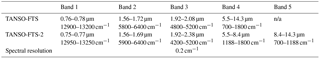
GOSAT-2 is due to be launched in Japan's 2018 financial year and is a follow-on from the original GOSAT mission launched in 2009. GOSAT-2, like GOSAT, is a collaborative effort between the Ministry of the Environment (MOE), the Japan Aerospace Exploration Agency (JAXA) and the National Institute for Environmental Studies (NIES) in Japan. GOSAT-2 aims to continue the legacy of GOSAT by providing global measurements of methane and carbon dioxide in order to monitor GHG emissions as well as new scientific data focusing on localised flux and point source emissions. GOSAT has an established history of providing reliable methane products (Parker et al., 2011; Schepers et al., 2012; Yoshida et al., 2011). GOSAT-2 represents one of the best opportunities for measuring methane isotopologues with this new generation of GHG satellite instruments. With the combination of the GOSAT and GOSAT-2 satellites, there will be a nearly unbroken record of global GHG emissions between 2009 and 2022 (with a 5-year lifetime planned for GOSAT-2), providing an unprecedented record on GHG emissions. The TANSO-FTS-2 instrument is similar to the TANSO-FTS instrument (Kuze et al., 2009) but, in the context of this study, has a significant advantage, which is the extension of band 3 up to 2380 nm, where significant numbers of methane spectral lines are located (Table 1). Therefore, this study focuses on the original GOSAT SWIR sensitivity region of 1560–1690 nm (band 2, also present in GOSAT-2) and the new SWIR sensitivity band in order to maximise any potential information on methane isotopologues. The exact technical details of GOSAT-2 are not yet available, but, due to the similarity of the instruments, we assume that the signal-to-noise ratio (SNR) and instrument line shape function (ILSF) on GOSAT-2/TANSO-FTS-2 and GOSAT/TANSO-FTS are similar; they are explained in more detail below (GOSAT-2 Project Team, 2017).
In order to identify the figures of merit that will be used for ICA in this study, we must first briefly outline the theory behind OEM. OEM theory was originally published by Rodgers (2000) and in the case of this study we use the interpretation of Yoshida et al. (2011). However, in the case of ICA, there is no retrieval step included since we make the assumption of evaluating the ICA at the linearisation point (the a priori vector).
OEM theory is fundamentally based on the estimation of the state vector (atmospheric profile) x given a set of measurements y. This relationship is typically expressed as
where F(x,b) is the forward model relating the atmospheric state to the measurements, b is a model parameter vector necessary for computations but is not retrieved and ε is an error vector comprising forward model errors and instrument errors. The optimal estimate (solution) for x using a non-linear maximum a posteriori method is achieved through minimising the cost function:
where xa is the a priori state of x, Sa is the VCM about the a priori state, and Sε is the error covariance matrix. However, since this section of the analysis does not include a retrieval step, we can linearly solve Eq. (3) as follows:
where K is the Jacobian matrix (or weighting function), defined as the derivative of the forward model as a function of the state vector, and is quantitatively defined as . The Jacobian matrix effectively describes the sensitivity of the forward model to changes in the state vector. G represents the Gain matrix, which describes the sensitivity of the final retrieved state vector to changes in the measurements; it is quantitatively described as
where the subscripts x and c refer to sub-matrices for target species (in this case 13CH4) and auxiliary/interfering elements respectively. Using these relationships we can define an information quantity, the “averaging kernel”, as
where is the a posteriori estimate of the state vector. The averaging kernel quantitatively describes the sensitivity of the final retrieved state vector to changes in the true state vector. In other words, in the context of this study, if we assume the true state vector is the a priori state, then the averaging kernel describes the ability of the retrieval to infer deviations in state vector elements away from the a priori state. Thus if A were an identity matrix it would represent a perfect retrieval, since all elements of the state vector would reproduce any changes with no interference. Given this fact the trace of A indicates the number of independent pieces of information a retrieval provides, otherwise known as the degrees of freedom for signal (DOFS), quantitatively described:
Thus in order to obtain relevant information out of a retrieval, the DOFS value must be greater than or equal to unity with each diagonal element of the averaging kernel representing a partial degree of freedom attached to a specific atmospheric layer, for a specific atmospheric parameter. The averaging kernel does not provide information on the expected errors in the 13CH4 channels, and therefore we must define a total error covariance matrix of the “retrieval state”. The total error covariance is defined as the sum of the measurement noise Sm, smoothing error Ss and interference error Si, and each of these quantities are defined below:
where Se is an ensemble a priori covariance matrix and the subscripts x and c denote the sub-matrices for target gases or auxiliary elements respectively.
The impact of these covariances is indicated in Yoshida et al. (2011) for 12CH4, the main methane molecule, where measurement and smoothing error form the main components of the error. The impact of the errors on any potential retrievals on 13CH4 is discussed below.
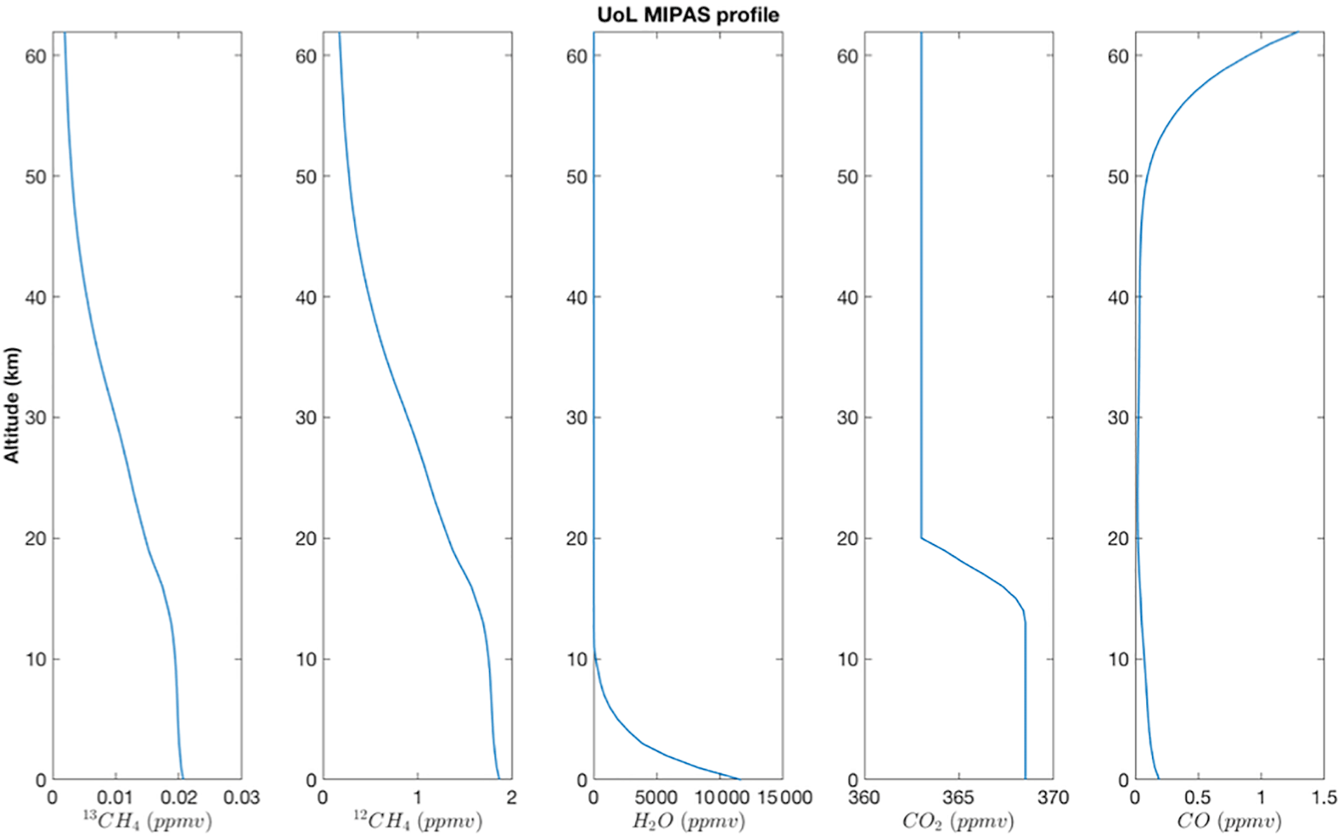
Making use of the ORFM, simulated unpolarised SWIR radiance spectra are generated based on an atmospheric model created at the University of Leicester for operational processing of the MIPAS instrument. The model provides a high level of vertical resolution and gas concentrations at 2002 estimates. This model is used throughout this paper and is designed to simulate mid-latitude daytime conditions (example profiles are shown in Fig. 2). The model does not have concentration values for 13CH4, and therefore a profile was generated based on the HITRAN 13C ∕ 12C ratio, which is 1.11031 % of the methane column. This paper generates vertical a priori state vectors based on this model, assuming a 21 level atmosphere between 0 and 63 km, with a high density in representation in the troposphere, and sparse representation (2–3) in the stratosphere, since SWIR are far more sensitive nearer the surface. It should be noted that Yoshida et al. (2011) use 15 atmospheric levels and Parker et al. (2011) employ 20.
4.1 A priori and its error covariance
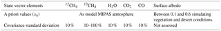
The a priori error covariance matrix can be generated based on transport models such as the NIES TM (Saeki et al., 2013) or from in situ data such as from the TCCON. There are many examples of appropriate covariance matrices for the purpose of GOSAT-based trace gas measurements (Eguchi et al., 2010; Yoshida et al., 2011), but there are no examples of 13CH4 a priori error covariance matrices in the established literature nor are there any transport models that can provide reliable values at this time. It was, therefore, necessary to experiment with a number of matrices in order to establish a covariance matrix that would provide sufficient information on the GOSAT-2 channels. The starting point for these matrices is based on the assumption that the maximum variations on δ13C that are likely to be observed, ranging from −10 to −80 ‰ (Rigby et al., 2012; Sherwood et al., 2016). Therefore, we can assume that the average global variation of δ13C is −45 ± 35 ‰. Applying Eq. (1), we can determine that a per mil variation of 35 equates to roughly (3 %)2 variance in the 13CH4. We accept that this is a very rough approximation, but it is effective in estimating a covariance starting point for 13CH4.
However, this variance represents a significant hurdle for 13CH4 retrieval. Even a priori covariance for methane retrievals from GOSAT is often not this restrictive. Eguchi et al. (2010) show examples of methane covariance at this magnitude level, but this is based on high levels of climatology analysis at which point the total column methane retrieval is closer to the a priori than to the satellite retrieval. Therefore algorithm developers often allow more variance in their covariance matrices in order to allow for more variation in the retrieved solution. Even with a more relaxed covariance matrix the DOFS on GOSAT retrievals are normally between 1 and 2. Given that 13CH4 is roughly 1.1 % of the methane signal and that total column retrievals are highly sensitive to the covariance matrices, it seems very unlikely that setting a 13CH4 covariance matrix to values of (3 %)2 or even (10 %)2 would yield any DOFS in the total column. We therefore deemed it necessary to allow the covariance to vary more significantly than this in order to establish the point where DOFS > 1, at the cost of increased a priori and a posteriori errors. Our assumption is that any retrieved 13CH4 variances can be averaged out, spatially and temporally. Therefore, this study initially assumes a (10 %)2 variance.
This study defines two forms of the matrix: firstly, a pure diagonal covariance matrix based on the equation
where Sa,ii is element ii (atmospheric layer) of a diagonal matrix, σa,i is the standard deviation of element i of the a priori vector, which in the case of this assessment is initially set at (10 %)2, and f is a scaling factor designed to increase or decrease the standard deviation of the elements of the covariance matrix. This factor f is designed to determine at what point the inherent instrument noise no longer has any influence on the retrieval. Because 13CH4 is present in minimal quantities in the atmosphere, it was deemed necessary to explore the effects of a non-diagonal covariance matrix, where the off-diagonal elements are calculated using the equation (Illingsworth et al., 2014):
where Sa,ij refers to a given off-diagonal element of layer ij, zi is the altitude of element i, zj is the altitude of element j and zS is the smoothing length, nominally set between 1 and 3 km. Off-diagonal elements describe the relationships between each of the pressure and altitude levels and are not always necessary in trace gas retrieval. This is especially true in cases such as CO2, which are highly stable in the atmosphere, and such knowledge is not needed. However, in the case of methane (and especially low-concentration gas such as 13CH4) it is important to determine the pressure level effects, since this could lead to large changes. Including off-diagonal elements will increase algorithm computation time but will likely result in a more accurate solution.
The other key gases present in bands 2 and 3 of GOSAT-2 (12CH4, CO2, H2O and CO) are all set at (10 %)2 of the MIPAS atmospheric profile, matching the initial value of the 13CH4 covariance matrix, with Herbin et al. (2013) suggesting similar variations at their peak.
The MIPAS model assumes a total column-averaged methane concentration of 1740 ppbv, which, assuming a 13C ratio of 1.1 %, equates to a total column-averaged concentration of 19.14 ppbv for 13CH4.
The ICA a priori set-ups and simulation set-ups are summarised in Table 2 below following the style of Herbin et al. (2013).
Variations are based on those values shown by Eguchi et al. (2010) and Herbin et al. (2013) but at their maximum, with the aim of determining the maximum interference error for 13CH4 for maximum DOFS.
4.2 Measurement error covariance matrix
Instrument performance is a crucial component of any ICA, but in the case of GOSAT-2/TANSO-FTS-2 the exact details of the FTS performance are not yet published. Therefore, ILSFs and SNR values equivalent to GOSAT/TANSO-FTS are assumed, purely for the SWIR bands. The assumed SNR is a factor of multiple components of the instrument and in the SWIR is a combination of inherent instrument noise (dark current) and noise from received photons (shot noise). Assuming varying land surface types and solar zenith/viewing zenith angles (from vegetation to desert), GOSAT has an SNR range between 300 and 500 (Yoshida et al., 2011) over band 2 (potentially lower over water surfaces); for the purposes of this study similar SNR values are assumed for band 3, taking into account the lower radiance values of band 3. Based on this knowledge, the instrument error covariance matrix is defined as
where
where σε,i is the standard deviation of the ith measurement of the measurement vector y. The diagonal values of the covariance matrix are identical since the SNR is applied to the entirety of the measurement bands rather than individual measurement values.
We note that additional errors can be incorporated into the measurement error covariance matrix, most notably errors from the forward model which can be due to incorrect physics approximations or errors in spectral line positions and many others; however, in the case of this study we assume that the majority of the errors are to be found in the instrument and forward model errors are not important. In the case of a full retrieval, forward model errors must be accounted for in order to make accurate measurements, but in the case of information content determination we are justified in ignoring them as they will not impact the information content to any significant degree (Frankenberg et al., 2012; Herbin et al., 2013).
4.3 Non-retrieved elements
The complexity of atmospheric retrievals requires that we consider the potential impact of elements outside the main retrieval parameters (b in Eq. 2). These quantities have not been included in the equations identified above since it is beyond the scope of this work, but the potential effects are described in detail in this section. Yoshida et al. (2011) put particular emphasis on potential instrumentation effects (outside those contained within the SNR) that are important to include in the retrieval vector, such as the wavenumber dispersion (an effect of self-apodisation and other effects). However, although we expect such effects to be present in TANSO-FTS-2, we judge that they are not important in the context of information content and are therefore not further considered in this work.
As highlighted in Yoshida et al. (2011), the GOSAT SWIR channels are polarised and it is intended for GOSAT-2 to contain polarised channels as well, but for this study we will assume that the “P” and “S” components have been combined to form a non-polarised spectrum, since the primary aim of the polarisation is to study atmospheric scattering and this is less important in this study, especially in the application of the proxy method.
We assume in this study that measurements are only made over land surfaces, and thus other state vector elements required to make retrievals over water surfaces (such as wind speed) are not considered. We choose to ignore the specular reflectance effects of the sea since this requires a far more complex model than the Lambertian model employed by Yoshida et al. (2011) and thus will add additional computation time. Logically if there is not enough information present in high albedo land surface conditions such as deserts, then water glint reflectance is unlikely to have a positive impact.
In the TIR waveband, physical effects such as surface emissivity and total column temperature variations can have significant effects on retrievals, but this work purely focuses on the SWIR, and thus such elements are not considered in this study.
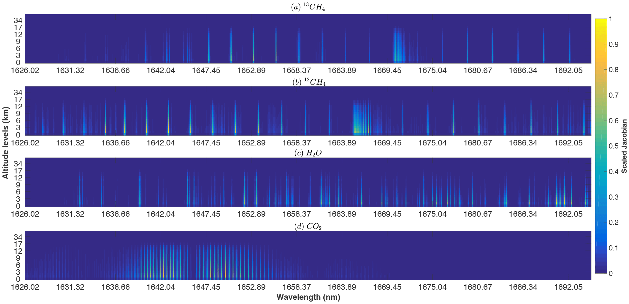
Figure 3Normalised sensitivity (between 0 and 1) of GOSAT-2 measured radiance with respect to a variation of 1 % of the concentration of the main constituent gases in the 1626–1692 nm (band 2) wavelength range; 13CH4 (a), 12CH4 (b), H2O (c) and CO2 (d). All calculations were performed using the ORFM RTM, assuming a solar zenith angle of 30∘, a viewing zenith angle of 0∘ and a surface albedo of 0.1, in conjunction with the HITRAN2012 database and the University of Leicester model MIPAS atmosphere.
Clouds and aerosols can severally impact accurate measurements of methane; for the purposes of this study, we assume that all retrievals are from clear sky and unaffected by clouds and that any impact from aerosols is largely negated by the aforementioned proxy effect, thereby negating any need to account for aerosols in the light path.
Given the sparseness of methane isotopologue lines, it is important to initially consider the relative sensitivity of the isotopologue lines in comparison to the interfering gases in the same spectral regions in both bands 2 and 3. These sensitivities are calculated from the Jacobean elements for each layer of the atmosphere using the ORFM tool and the HITRAN2012 database as a basis for these calculations. All simulations were run at a 0.01 cm−1 spectral resolution and then convolved with a GOSAT/TANSO-FTS ILSF downloaded from the GOSAT Data Archive Service (https://data2.gosat.nies.go.jp/).
Initial consideration is given to band 2, where solar irradiance is at a maximum for TANSO-FTS-2. Figure 3 shows the scale of the task at hand, with very few spectral lines of 13CH4 present in this particular waveband, with only a handful indicating significant sensitivity. We note that the 13CH4 spectral lines exhibit similar behaviour to the 12CH4 spectral lines but are phase shifted by several nanometres, which is a characteristic of similar rotational–vibrational bands at different transition energies. This spectral region is known as the “tetradecad” region and 13CH4 absorption is dominated by the 2ν3 vibrational band, and 12CH4 in this region is characterised by more complex rotational–vibrational states, which are described in more detail in Brown et al. (2013) and Lyulin et al. (2010). It is important to note that Brown et al. (2013) issue warnings that significant uncertainties are still attached to the quantum positions of the methane isotopologue lines, especially relating to the effects of atmospheric broadening. This is less applicable to the wave range shown in Fig. 3 but should still be considered, as it suggests that uncertainty values must be ascribed to the centre position of the isotopologue lines. The methane lines in this region were significantly updated from the previous iteration in HITRAN2008 (Rothman et al., 2009) and were specifically recorded using pure 13CH4 and differential absorption spectroscopy (Lyulin et al., 2010). They are judged to be accurate, but Brown et al. (2013) note that “the new HITRAN list of 13CH4 above 6170 cm−1 is believed to be incomplete”, suggesting that there are additional lines in band 2 that could be leveraged in future HITRAN iterations. Figure 3 identifies that both 12CH4 and 13CH4 radiance sensitivity peaks at roughly the same altitudes (about 3 km) and remain sensitive up until the mid-troposphere. These results suggest that the transitions of the isotopologues are at similar lower-state energy levels and are therefore affected by atmospheric phenomena such as temperature changes in similar fashions, contrasting with the sensitivities of carbon dioxide isotopologues as evidenced by Reuter et al. (2012). The MIPAS model atmosphere shows water vapour concentrations dropping off very quickly with increasing altitude, and the sensitivity of water vapour in Fig. 3 shows significant variation in the altitudes at which water vapour is sensitive; however, it also shows significant water vapour spectral lines in this spectral range, suggesting that significant interference errors due to water vapour in the lower portion of the atmosphere can be expected. Carbon dioxide also has a significant presence in this waveband, showing similar sensitivities to the main methane isotopologues.
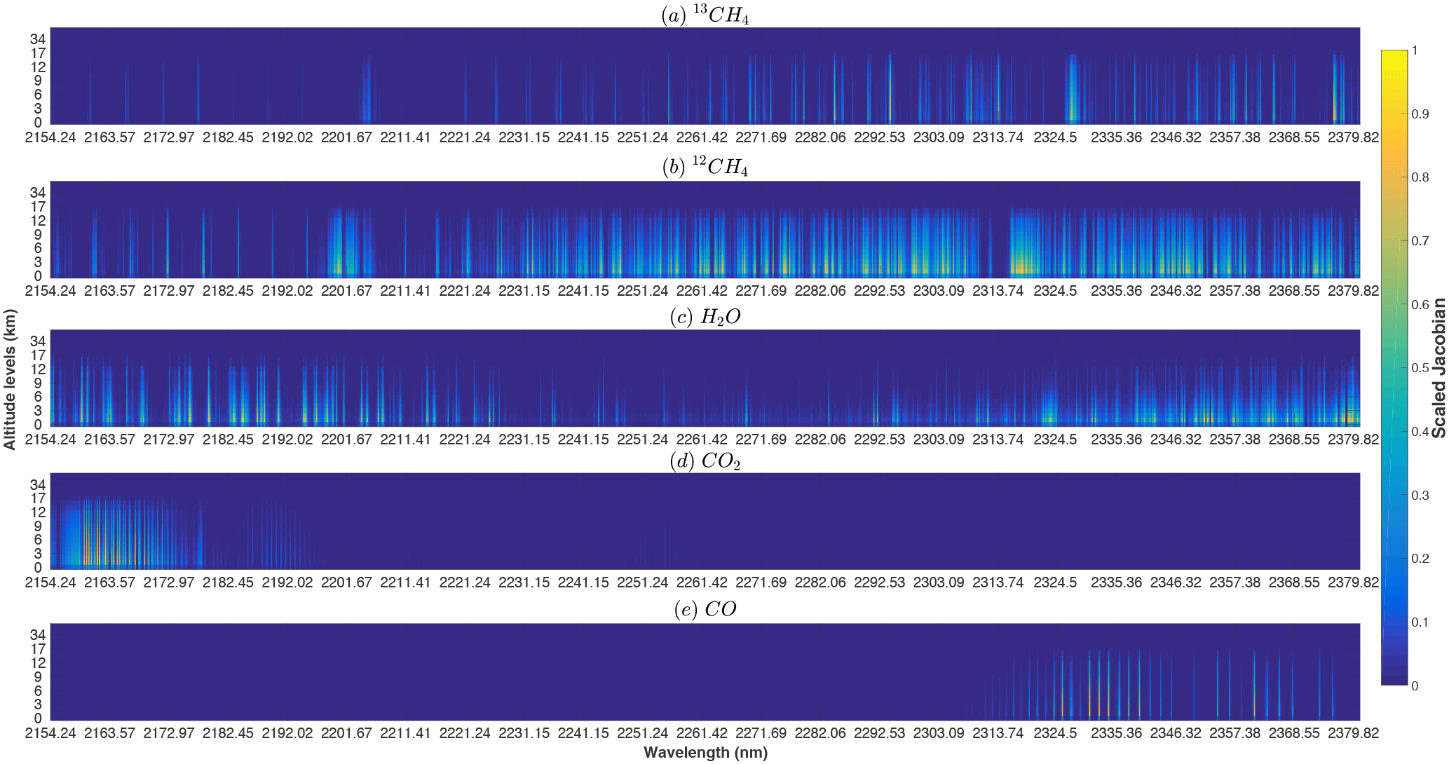
Figure 4Normalised sensitivity (between 0 and 1) of GOSAT-2 measured radiance with respect to a variation of 1 % of the concentration of the main constituent gases in the 2154–2380 nm (band 3) wavelength range; 13CH4 (a), 12CH4 (b), H2O (c), CO2 (d) and CO (e). All calculations were performed using the ORFM RTM, assuming a solar zenith angle of 30∘, a viewing zenith angle of 0∘ and a surface albedo of 0.1, in conjunction with the HITRAN2012 database and the University of Leicester model MIPAS atmosphere.
Consideration is now given to a portion of TANSO-FTS-2 band 3 waveband, specifically the portion where methane spectral lines are particularly common (Fig. 4). Band 3 clearly has significantly higher levels of spectral lines for methane than band 2, although a wider waveband is considered since methane is present in only a very narrow spectral region of band 2. 12CH4 is particularly prevalent in this region, showing high levels of sensitivity especially in the lower troposphere and in the boundary layer, while 13CH4 lines are relatively dense and generally show low sensitivity except for a handful of lines. Sensitivity to the surface layer is well documented (Yoshida et al., 2011; Herbin et al., 2013) and, like band 2, band 3 should be able to maximise measurements in the surface level as opposed to higher up in the atmosphere, where TIR measurements tend to be more sensitive. We note that band 3 has lower solar irradiance values than band 2, and therefore lower radiance values from this region and lower SNR values are likely. This suggests that bands 2 and 3 have a trade-off between the number of spectral lines present in the range and the total SNR achievable by each band.
The rotational–vibrational states in this particular spectral region (or polyad) are defined as the “octad”, meaning that all 13CH4 transitions exist at lower energy levels than the tetradecad polyad of band 2 and that there are significantly lower numbers of transitions available in band 3 as opposed to band 2. The spectral lines for 13CH4 in band 3 are brand new in the HITRAN2012 database. All spectral lines were captured using FTIR measurements from the Kitt Peak facility and can be ascribed a high degree of confidence (Brown et al., 2013; Lyulin et al., 2010).
Table 3Description of scenarios undertaken to determine potential 13CH4 content in GOSAT-2/TANSO-FTS-2.
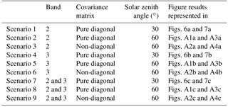
Based on the equations and methods outlined in Sect. 4, the primary aim of this work is to determine the potential information content of 13CH4 in GOSAT-2/TANSO-FTS-2. However, unlike other GOSAT information content studies such as Herbin et al. (2013), there are no previous studies indicating the ideal retrieval set-up (i.e. surface or solar conditions, a priori state vectors). Therefore we are required to experiment in order to determine under what conditions there may be sufficient information available in the 13CH4 bands to allow for an effective retrieval. To determine the potential information content in the bands, the following scenarios were designed, with the specific goal of varying the a priori covariance matrix, with the scaling factor included in all scenarios and the solar zenith angle, to determine what effects varying the optical path length may have.
The scenarios listed in Table 3 aim to determine the level of information content available in each of the SWIR bands and a combination of the bands. In addition to solar zenith angle, surface albedo is taken into account in each of the scenarios, assuming a range of 0.1–0.6 (please see the ESA ADAM database for a comprehensive review of global surface albedos, based on MODIS data; available at http://adam.noveltis.com/), consistent with vegetation to desert surface conditions. We note that Yoshida et al. (2011) retrieve CH4, CO2 and H2O simultaneously; all gases are simulated to be retrieved simultaneously in this study as well. It is necessary to retrieve 12CH4 and 13CH4 simultaneously in order to define a δ13C value for any given retrieval. As identified in Sect. 4, the TANSO-FTS-2 SNR is modified in accordance with the surface type. All other information is constant as either specified in Sect. 4, or in the MIPAS model atmosphere (such as other gases or temperature profiles). Clear-sky conditions are assumed (i.e. no clouds or aerosols), and no modifications of the optical path are expected.
Results from scenarios 1, 4 and 7 are shown in Fig. 6 below. The results from scenarios 2, 5 and 8 are shown in Fig. A1 and scenarios 3, 6 and 9 are shown in Fig. A2, both of which are in the Appendix.
6.1 Band 2
Figure 6a shows the DOFS for 13CH4 assuming retrievals from band 2 of TANSO-FTS-2, assuming the conditions outlined in scenario 1 and the a priori covariance variability identified in Sect. 4. For an f factor (see Eq. 11) of 1, equating to a (10 %)2 variability in the covariance matrix, Fig. 6a suggests that an average of 0.1 DOFS can be expected for surface albedo conditions varying between 0.1 and 0.6, suggesting any information for such a covariance matrix is strongly dependent on the a priori rather than the measurement. This is likely to be a product of the low concentrations of 13CH4 in the atmosphere. Figure 6a suggests that retrievals in band 2 for 13CH4 is difficult, with only high albedo surface conditions giving the potential for unity values of DOFS, and even this only occurs when the f factor is equal to 10 or over, equating to (100 %)2 variability in the covariance matrix. As a comparison, Yoshida et al. (2011) show that DOFS of up to 2 for high albedo conditions are achievable for methane retrieval, with a covariance matrix roughly equivalent to (∼ 10 %)2 variability, using TANSO-FTS. These results add to the weight of evidence that implies the difficulty of operational retrieval of 13CH4. The maximum DOFS obtainable with band 2, assuming scaling factors up to the value 10, with the scenarios outlined in Table 3 are summarised in Table 4 below, and the related figures are shown in the Appendices below (Figs. A1a and A2a).
The results shown in Table 4 suggest that solar zenith angle is not an important factor in retrieval for band 2 (in relation to 13CH4 rather than methane). This is most likely because the optical depth of 13CH4 is so low that changing the solar zenith angle does not change the 13CH4 air mass significantly. In order to highlight this point, we include an ORFM simulation of optical depth for two narrow wavelength ranges in band 2 of TANSO-FTS-2 (Fig. 5), which clearly shows very low optical depth values.
There may be some benefit to extreme solar zenith angle and large viewing zenith angles, but if significant information can only be obtained at special geometries then this instantly removes the vast majority of GOSAT-2 measurements as beneficial. The inclusion of “off-diagonal” values into the covariance matrix improves the information content of the signals; in the case of a high scale factor, DOFS values of unity are obtained for all surface albedo values (see Fig. A2a), with unity being achieved for a scale factor of 5 ((50 %)2 variance) for an albedo value of 0.6. Even with this best-case scenario, as a single measurement, this is not significantly beneficial and will not allow for an accurate value of δ13C to be calculated nor allow for conclusions to be drawn about the nature of the source of the measurement. Overall, measurement variance can be decreased by averaging many measurements over large spatial regions or temporal periods, at the cost of high seasonal or spatial resolution.
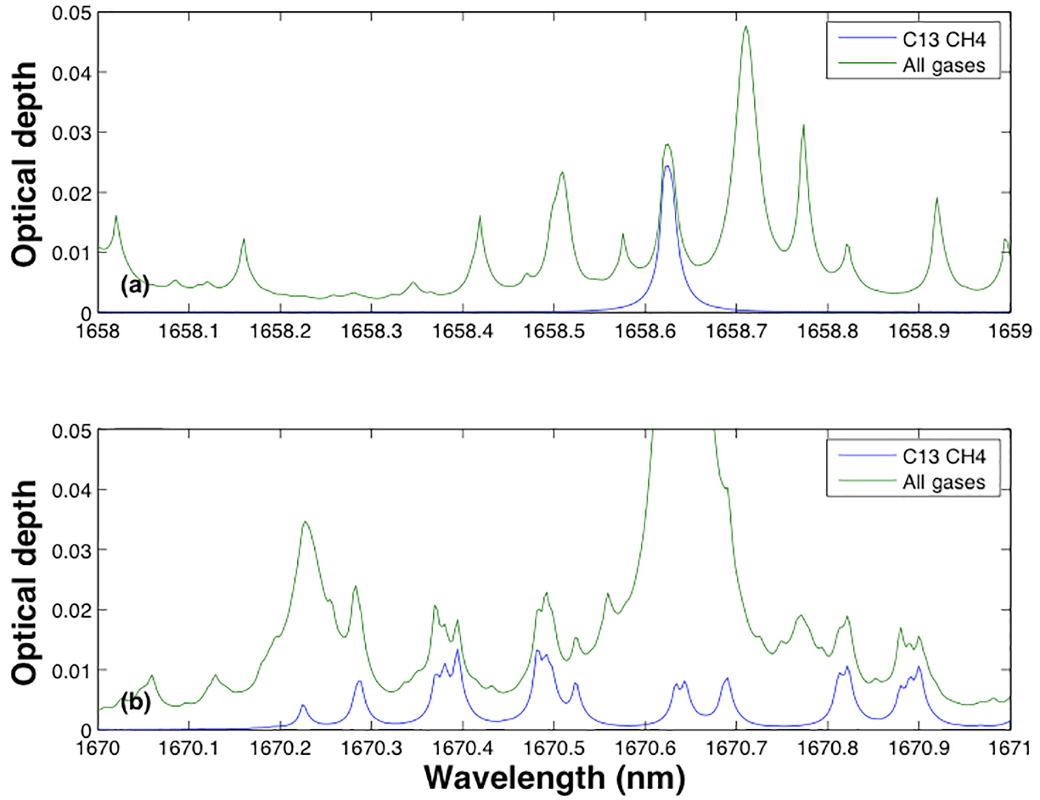
Figure 5Optical depth covering two narrow 13CH4 spectral regions in band 2 of TANSO-FTS-2: the green line represents optical depth of all gases present in this portion of the spectrum (CH4, CO2 and H2O), whilst the blue line shows optical depth of purely the methane isotopologue 13CH4: panel (a) indicates optical depth in the wavelength range 1658–1659 nm; panel (b) shows optical depth in the wavelength range 1670–1671 nm.
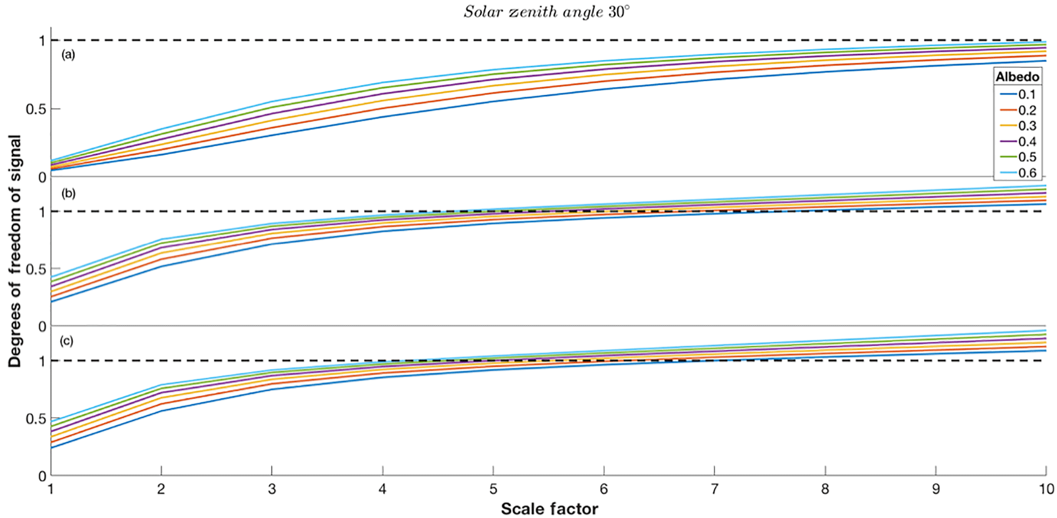
Figure 6Degrees of freedom for signal for 13CH4 vs. scaling factor f for scenarios outlined in Table 3. Each coloured line represents different surface albedo conditions as shown in the key. The black dashed line represents unity DOFS: panel (a) indicates scenario 1, panel (b) indicates scenario 4 and panel (c) indicates scenario 7.
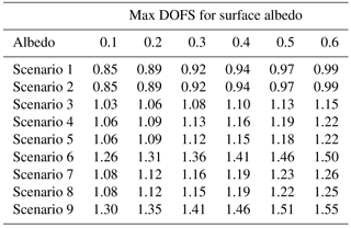
Table 4Summary of DOFS characteristics for all scenarios' six surface albedos.
6.2 Band 3
Figure 6b shows the DOFS for 13CH4 assuming retrievals from band 3 of TANSO-FTS-2, assuming the conditions outlined in scenario 4 and the a priori covariance variability identified in Sect. 4. Figure 6b suggests that an average of 0.3 DOFS can be expected for surface albedo conditions varying between 0.1 and 0.6 when assuming a variance of (10 %)2. This is an improvement on the DOFS suggested by band 2, but not by a significant amount. Again this suggests that any information for such a covariance matrix is strongly dependent on the a priori rather than the measurement. However, we note that unlike the results shown in Fig. 6a, DOFS values of 1 can be expected above a scale factor of 7 for all albedos shown, suggesting that definitive information from band 3 for 13CH4 can be expected and is not reliant on extremely high surface albedo conditions, which will be rare on the surface of Earth at these wavelengths. However, the required scale factor is still high and, given this level of variance, significant spatial and temporal averaging is most likely required. The results from the remaining band 3 scenarios are shown in Table 4 and Figs. A1b and A2b.
Like band 2, changing the solar zenith angle does not have a significant impact on the DOFS available for 13CH4 retrieval. However, the addition of “off-diagonal” elements to the a priori covariance matrix has a significant impact on the available DOFS as highlighted by Fig. A2b, which suggests that information can be extracted from a total column for all surface albedos at a scaling factor of 4 (40 %)2, increasing to a factor of 2.5 (25 %)2 when only considering high surface albedo values. It is clear that band 3 of TANSO-FTS-2 has significant benefits over band 2 in terms of information content; even without exactly fixed instrument noise or a priori state vectors and covariance matrices, there is a clear benefit in retrieving 13CH4 in this band. However, the results suggest that significant variance is still required in order to guarantee the solution to the OEM is based on the measurements rather than the a priori. Therefore substantial temporal and spatial averaging is likely to be required in the same manner as band 2.
6.3 Combined band 2 and band 3
The dual detector nature of the future SWIR bands of GOSAT-2 allows for a combination of the information channels of bands 2 and 3 in order to maximise information content. Because both bands are based on solar backscatter measurements, and largely contain the same interfering elements, there is no issue with a direct combination. In contrast, TIR elements which are sensitive to different portions of the atmosphere are difficult to combine directly with SWIR measurements (Herbin et al., 2013). The pure application of this concept increases calculation time significantly due to the number of spectral lines present in both bands. However, full retrievals are not the main aim of this work as opposed to determining maximum information content in the GOSAT-2 bands; therefore we are justified again in making retrieval speed a low priority.
The results identified in Fig. 6c show some differences between the application of spectral lines in band 3 and those in band 2 and band 3. Although these differences are minor, there is a definite increase in DOFS of roughly 0.1 for each of the scaling factors. We also note that the spread of the DOFS lines due to varying albedo conditions are more widely spaced as compared to band 3 DOFS, suggesting that measurements in the combined bands are more sensitive to surface conditions. The degree to which the DOFS increases w.r.t. the scaling factor is sharper than in band 2 so that DOFS values of unity are achieved for all albedo values at scaling factor 7, a variance of (70 %)2. These values suggest that retrieval of 13CH4 is feasible within the operational lifetime of GOSAT-2. This is further emphasised by the results from the other bands 2 and 3, summarised in Table 4 below and Figs. A1c and A2c.
Table 4 shows the same trends as the DOFS results shown in bands 2 and 3 individually, in that the solar zenith angle has a minor impact on the DOFS, and the variation of the a priori covariance matrix has a similar scaling effect on the DOFS. Yet the combination of both bands has yielded a modest increase in the DOFS for all scenarios at all surface albedos. Considering the “off-diagonal” a priori case in scenario 9 we find that DOFS equal to unity are achievable for all surface albedo type at a scaling factor of 3.5 (35 %)2, which is clearly superior to any of the other cases considered in this paper. Therefore there are significant benefits to dual band retrievals with TANSO-FTS-2. However, it is important to note that combining the two bands led to a significant computational cost (roughly 3 times longer than considering each band independently) and is possibly not practical for full-scale retrievals in the form identified in this paper. However, note that the code used in this study was not optimised for retrieval and was designed purely for this analysis. Therefore an optimised retrieval code should be able to cut this computation time down significantly.
All the maximum achievable DOFS results from all scenarios are outlined in Table 4 below.

Figure 7Synthetic total column retrieval errors for scenarios outlined in Table 3, based on Eqs. (8), (9), (10) and (16). The maximum and minimum values (based on maximum and minimum SNR) for interference, measurement and smoothing error are shown, in addition to the total error: panel (a) indicates scenario 1, panel (b) indicates scenario 4 and panel (c) indicates scenario 7.
Even if sufficient DOFS can be established to identify where 13CH4 retrievals are influenced more by the measurement than by the a priori, the errors associated with the retrieval may well make identifying methane source types a practical impossibility. Therefore an assessment of the expected total column errors is required; these errors for 13CH4 can be summarised as (Yoshida et al., 2011)
where σ is the total column a posteriori error, depending on the subset of altitudes or pressures used, h is the dry air partial column, calculated from n layers of the retrieval grid (21 in this case), and wdry is calculated from the model pressure profile and H2O concentration profile. 1 is a column vector with elements of unity and a length equivalent to the dry air partial column.
Using the scenarios outlined in Table 3, the total column error (along with the interference, smoothing and measurement errors) for 13CH4 retrieval can be established. Total column errors for 12CH4 are assumed to be documented in studies such as Parker et al. (2011) and Yoshida et al. (2011).
Results from scenarios 1, 4 and 7 are shown in Fig. 7 below. The results from scenarios 2, 5 and 8 are shown in Fig. A3 and scenarios 3, 6 and 9 are shown in Fig. A4, both of which are in the Appendix.
7.1 Band 2
Based on the summation of errors identified above, we can estimate the precision of a synthetic retrieval in band 2 of TANSO-FTS-2, for the range of a priori covariance matrices identified previously.
Scenario 1 (Fig. 6a) suggests that retrievals are heavily biased towards the a priori in band 2 of TANSO-FTS, except perhaps for a variance of (100 %)2 over a very bright surface (i.e. albedo of 0.6, or SNR equal to 500). In this case, the maximum precision for a single sounding equates to 2.4 ppbv for 13CH4. Based on the total column-averaged concentration of 13CH4 from the MIPAS profile identified in Sect. 4.1, 2.4 ppbv precision equates to roughly 13 % error. For reference, Yoshida et al. (2011) show that the average total column precision for methane retrievals is 5.86 ppbv, which equates to 3.4 %. Based on the DOFS values for scenario 2 (Fig. A1a), we can assume similar precision values, but the DOFS values for scenario 3 (Fig. A2a) suggest that unity is achieved for variance of (80 %)2 or above for the whole SNR range. Based on the error values shown in Fig. A4a, the maximum precision at this variance is 2.2 ppbv and the minimum is 3 ppbv, equating to 11.5 % and 15.6 % error respectively. These results are far from the base 0.2 ppbv precision requirement set in Sect. 2.2 (and especially far from the modified targets of 0.147 and 0.04 ppbv), but the precision can be increased through averaging multiple retrievals together (both temporally and spatially), where the standard deviation is inversely proportional to the square root of the number of measurements (Parker et al., 2015). Therefore, for scenario 3, we suggest that a precision of 0.2 ppbv can be achieved using the average of 121 measurements for high SNR and 225 measurements for low SNR, both of which are achievable over a significant period of time with a large spatial region for GOSAT-2. Taking into account 12CH4 uncertainty, which increases the 13CH4 precision requirements, we assume that when averaged over the numbers of measurements identified above we can expected a 12CH4 precision of 5 ppbv, equating to a required increase in 13CH4 precision to 0.147 ppbv which can be achieved using the average of 224 measurements for high SNR and 416 measurements for low SNR. These scales of measurements seem less likely to be achievable with the explicit goal of determining source types, but it may be possible to investigate globally averaged temporal trend climatology or hemispherical biases. Note that these metrics do not include the effects of any potential biases in the retrievals, which will not be removed through spatial and temporal averaging and can potential skew the assumed δ13C values.
7.2 Band 3
Using the methods identified above in band 2, the total errors for band 3 retrievals are explored.
Scenario 4 (Fig. 6b) shows that unity DOFS occurs for variance of (80 %)2 or above for the whole SNR range. Using Fig. 7b, we can suggest that the maximum and minimum precision is 1.5 and 1.8 ppbv respectively; these equate to 7.8 and 9.4 % of the total column. We suggest that through spatial and temporal averaging, these errors can be reduced to the 0.2 ppbv target by averaging 56 and 81 measurements for maximum and minimum SNR cases and, in the case of methane precision errors of 5 ppbv (104 and 150 measurements) and 15 ppbv (1400 and 2025 measurements). Changing the solar zenith angle for scenario 5 (Fig. A1b) does not impact the DOFS significantly, but, if we consider scenario 6 (Fig. A2b), DOFS of unity occur for variance of (40 %)2 or above for the whole SNR range. The maximum and minimum precisions at this variance are 1.1 and 1.3 ppbv (Fig. A4b) respectively. The target precision can be increased through averaging 20 and 28 measurements respectively and, in the case of 12CH4, precision errors of 5 ppbv (56 and 78 measurements) and 15 ppbv (756 and 1050 measurements). Therefore for retrievals with band 3, we suggest that measurements of δ13C to an accuracy of 10 ‰ can be achieved within monthly periods of GOSAT-2 measurements, assuming small levels of 12CH4 precision errors, which are achievable when averaged over large volumes of data. If we assume that there is a constant 5 ppbv or greater 12CH4 precision errors, then we suggest that δ13C for Transcom regional-scale analyses are more appropriate (Takagi et al., 2014). Again the potential for biases caused by systematic errors must be considered, with Sect. 2 suggesting that a minimum δ13C bias of 5 ‰ can occur.
7.3 Combined band 2 and band 3
Scenario 7 (Fig. 6c) shows that unity DOFS occurs for variance of (70 %)2 or above for the whole SNR range. Using Fig. 7c, we suggest that the maximum and minimum precision at this variance is 1.5 and 1.8 ppbv respectively, i.e. very similar to those found in band 3 scenario 4; therefore similar numbers of measurements are required in order to achieve the desired precision. If we consider scenario 9, unity DOFS are achieved for a variance of (35 %)2 (Fig. A2c); the maximum and minimum precisions at this variance are 0.7 and 1.2 ppbv (Fig. A4c) respectively. The target precision of 0.2 ppbv can be increased through averaging 12 and 36 measurements respectively and, in the cases of 12CH4, precision errors of 5 ppbv (23 and 67 measurements) and 15 ppbv (306 and 900 measurements). Scenario 9 shows the best results in terms of information content and measurement precision, to the point where over highly reflective surfaces very few measurements are required in order to make an accurate assessment of the source type.
The next step to performing retrievals of 13CH4 from GOSAT-2 is validating these measurements. This is currently a challenging topic since there are currently no total column measurements of 13CH4 in the public domain. As discussed in the Introduction, the only currently available measurements are available from NOAA flask data (Nisbet et al., 2016), land or airborne surveys of specific locations (Fisher et al., 2017), stratospheric balloon measurements (Röckmann et al., 2011) or ACE-FTS limb measurements (Buzan et al., 2016). These measurements only cover specific sections of the atmosphere and cannot be directly compared to any total column measurements. Having said this, comparisons can be made, with the caveat that biases will exist between the measurement techniques due to atmospheric circulation and/or fractionation. Studies that attempt this having adequately described what these biases could be would be a major step forward.
Another potential avenue is to modify currently existing global chemistry transport models to incorporate 13CH4 transport and fractionation. Based on surface measurements from NOAA flask data, this method could adequately represent total column 13CH4. Buzan et al. (2016) attempt this with the Whole Atmosphere Community Climate Model (WACCM) in order to compare against ACE-FTS measurements, with mixed results.
Finally the TCCON mentioned above is perhaps the most useful avenue for pursuit. Although 13CH4 measurements are not currently available from TCCON, some minor modifications to the standard GGG2014 algorithm should provide the appropriate utility. TCCON has spectral sensitivity to band 2 of TANSO-FTS-2 and, because TCCON retrievals are not dependent of solar backscatter, can obtain much higher SNR measurements.
This study has been performed largely with the JAXA/NIES/MOE GOSAT retrieval algorithm (Yoshida et al., 2011, 2013) in mind, with the hope that only minor modifications to the algorithm will allow for retrievals of 13CH4 from GOSAT-2. This of course extends to any other a priori based retrieval algorithm. However, there is an important argument to be made about the usefulness of a priori methods in the case of 13CH4 when such huge covariances are required in order to obtain information content. The operational methane algorithm on the recently launched TROPOMI uses the Phillips–Tikhonov regularisation scheme (Hu et al., 2016), which makes use of a regularisation parameter instead of a priori data or covariances. Because currently available schemes do not easy provide values for 13CH4 a priori data, the Phillips–Tikhonov may be a more suitable method for future algorithm development.
To summarise, this work investigates the possibility of whether 13CH4 can be retrieved with a sufficient level of accuracy by bands 2 and 3 of the GOSAT-2/TANSO-FTS-2 instrument via the use of the δ13C ratio in order to make a judgement on the nature of a methane source type (biogenic, thermogenic or abiogenic). We assume that an accuracy of 10 ‰ of δ13C values is sufficient to distinguish between methane source types, as shown by Rigby et al. (2012), and with this accuracy we calculate that a minimum 13CH4 retrieval precision of 0.2 ppbv is required in order to achieve δ13C with a 10 ‰ accuracy, but preferably 0.147 or 0.04 ppbv when taking into account precision errors on 12CH4.
Using the well-established DOFS methods (Rodgers, 2000), the RTM ORFM and the assumption of clear-sky conditions we calculate the key metrics of DOFS and total retrieval error in order to judge (a) the information content in a retrieval and (b) the precision of that retrieval, based on a series of test a priori covariance matrices. Using a combination of bands 2 and 3, we find that total column retrieval of 13CH4 with sufficient DOFS is possible, with a maximum and minimum precision of 0.7 and 1.2 ppbv respectively. Assuming statistical error reduction techniques, this precision can be increased to 0.2 ppbv by averaging over 12 and 36 measurements, to 0.147 ppbv by averaging over 23 and 67 measurements, and to 0.04 ppbv by averaging over 306 and 900 measurements respectively. This number of measurements for the best two target precisions is certainly achievable over a monthly period, assuming modest spatial sampling of 2∘ × 2∘, which is often how GOSAT data are represented. This implies that GOSAT-2 will be able to differentiate between methane source types at a high temporal resolution. However, in the case of high precision errors on 12CH4, representation of δ13C on Transcom regional scales is a more feasible prospect.
This analysis was also applied to bands 2 and 3 individually, and it was found that band 2 can achieve enough DOFS for a 13CH4 retrieval at the desired precision, based on averaging up to 225 measurements for a completely unconstrained a priori covariance matrix. Band 3 showed similar results to bands 2 and 3 combined but required up to 81 measurements in order to achieve the required precision. These are in the cases of no or limited 12CH4 precision error.
Across all bands, we find that the DOFS and precision are significantly affected by the instrument SNR but not by the solar zenith angle to any significant degree. In addition, the rate of increase of DOFS with respect to scaling factor is significantly higher in the combined bands than either band when considered individually. However, combining the DOFS from both bands leads to a significant computational penalty.
Given the relative abundance of 13CH4 spectral lines in band 3 of GOSAT-2, there is also some scope for future comparisons with measurements from Sentinel 5 and 5-P, both of which are sensitive to the same spectral regions. In addition, it is envisaged that there will be a period when GOSAT and GOSAT-2 are in simultaneous operation, and it may be possible to combine the measurements from both of these satellites in order to reduce uncertainty in isotopologue measurements.
The code and simulation parameters used in the course of this study are available by contacting the primary author. The ORFM RTM is available by contacting the main developer Anu Dudhia (http://eodg.atm.ox.ac.uk/RFM/). The GOSAT ILSFs are available from the following webpage (http://data2.gosat.nies.go.jp/doc/document.html\#Document). The HITRAN spectral database is available through the following website (http://hitran.org/), which requires specific user inputs.
The scenario plots not indicated in the main text are shown below, namely scenarios 2, 3, 5, 6, 8 and 9 for both DOFS and retrieval errors.
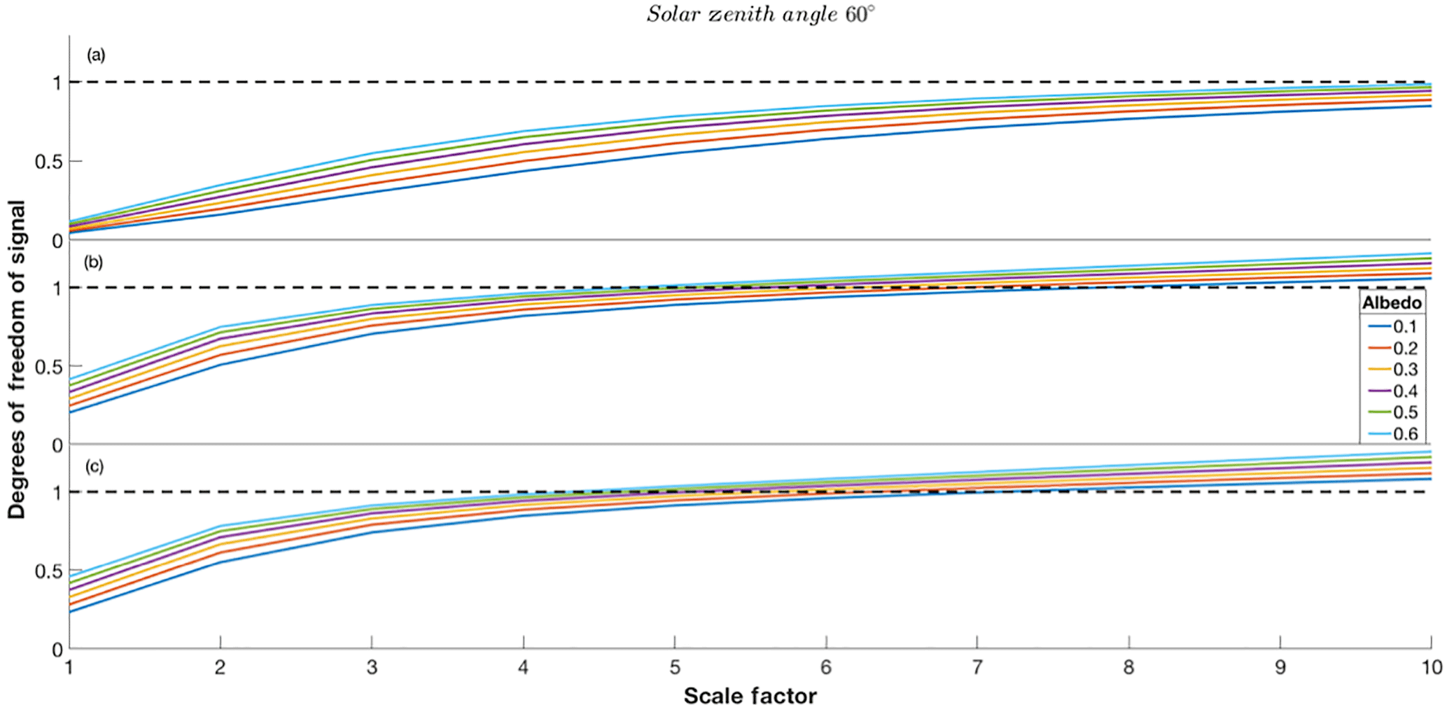
Figure A1Degrees of freedom for 13CH4 vs. scaling factor f for scenarios outlined in Table 3. Each coloured line represents different surface albedo conditions as shown in the key. The black dashed line represents unity DOFS: panel (a) indicates scenario 2, panel (b) indicates scenario 5 and panel (c) indicates scenario 8.
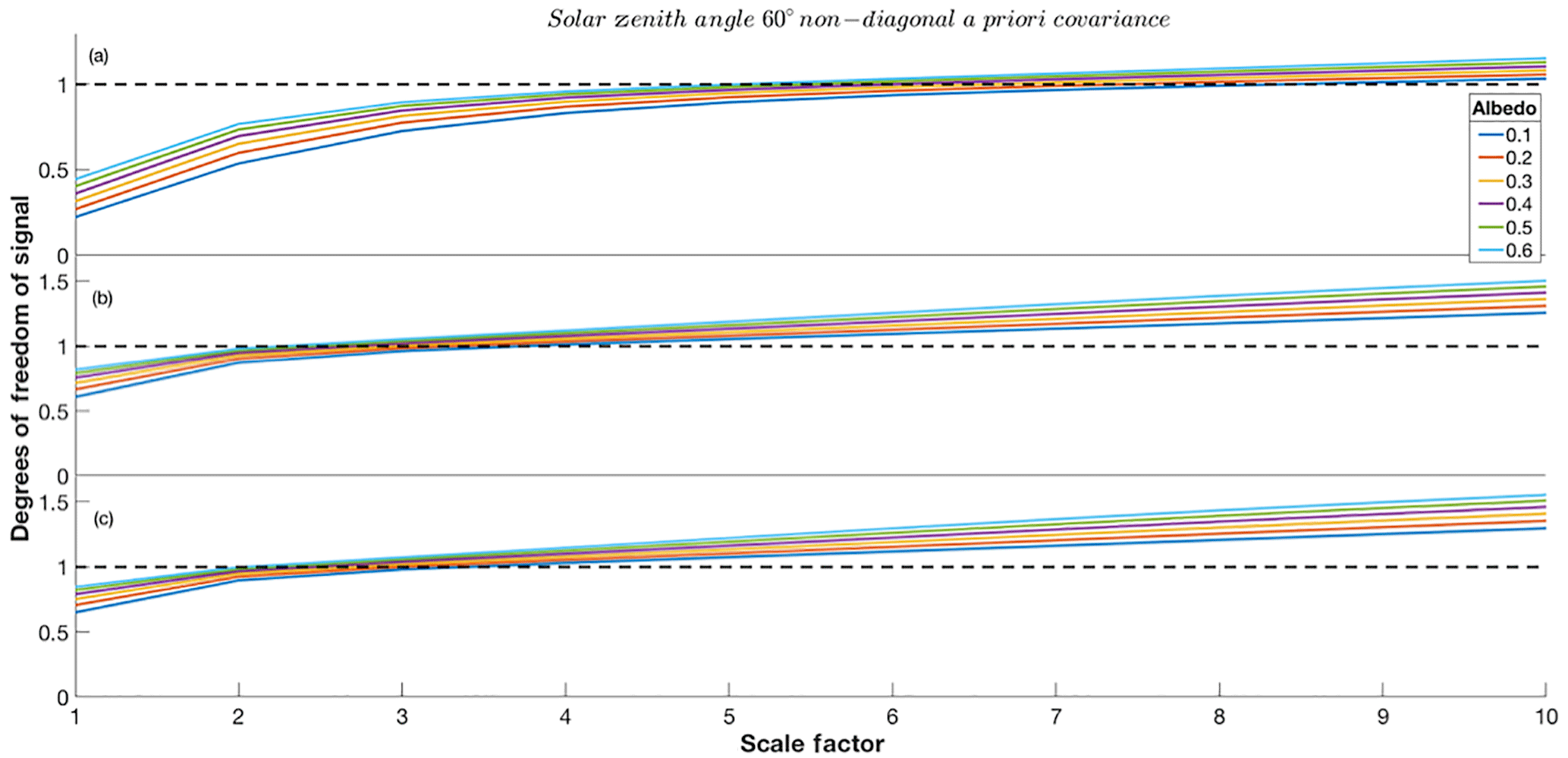
Figure A2Degrees of freedom for 13CH4 vs. scaling factor f for scenarios outlined in Table 3. Each coloured line represents different surface albedo conditions as shown in the key. The black dashed line represents unity DOFS: panel (a) indicates scenario 3, panel (b) indicates scenario 6 and panel (c) indicates scenario 9.
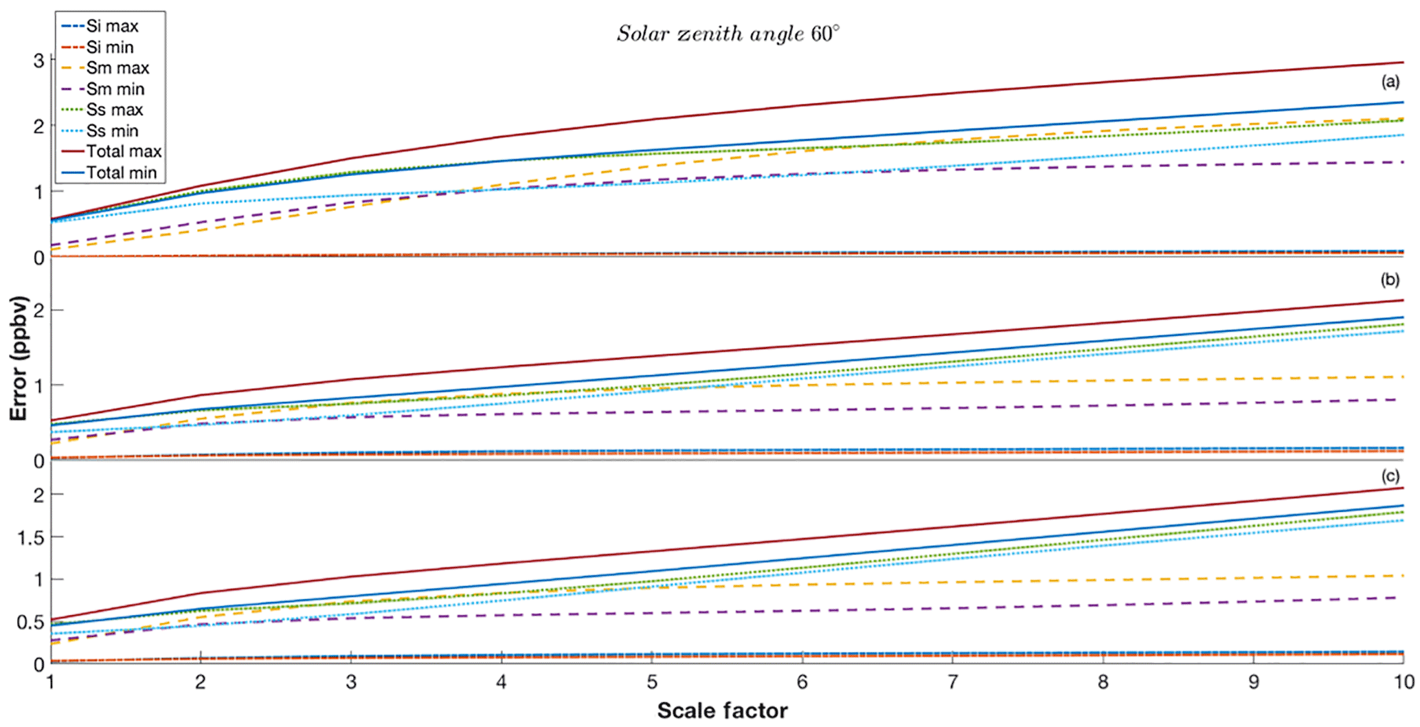
Figure A3Synthetic total column retrieval errors retrieval for scenarios outlined in Table 3, based on Eqs. (8), (9), (10) and (16). The maximum and minimum values (based on maximum and minimum SNR) for interference, measurement and smoothing error are shown, in addition to the total error: panel (a) indicates scenario 2, panel (b) indicates scenario 5 and panel (c) indicates scenario 8.
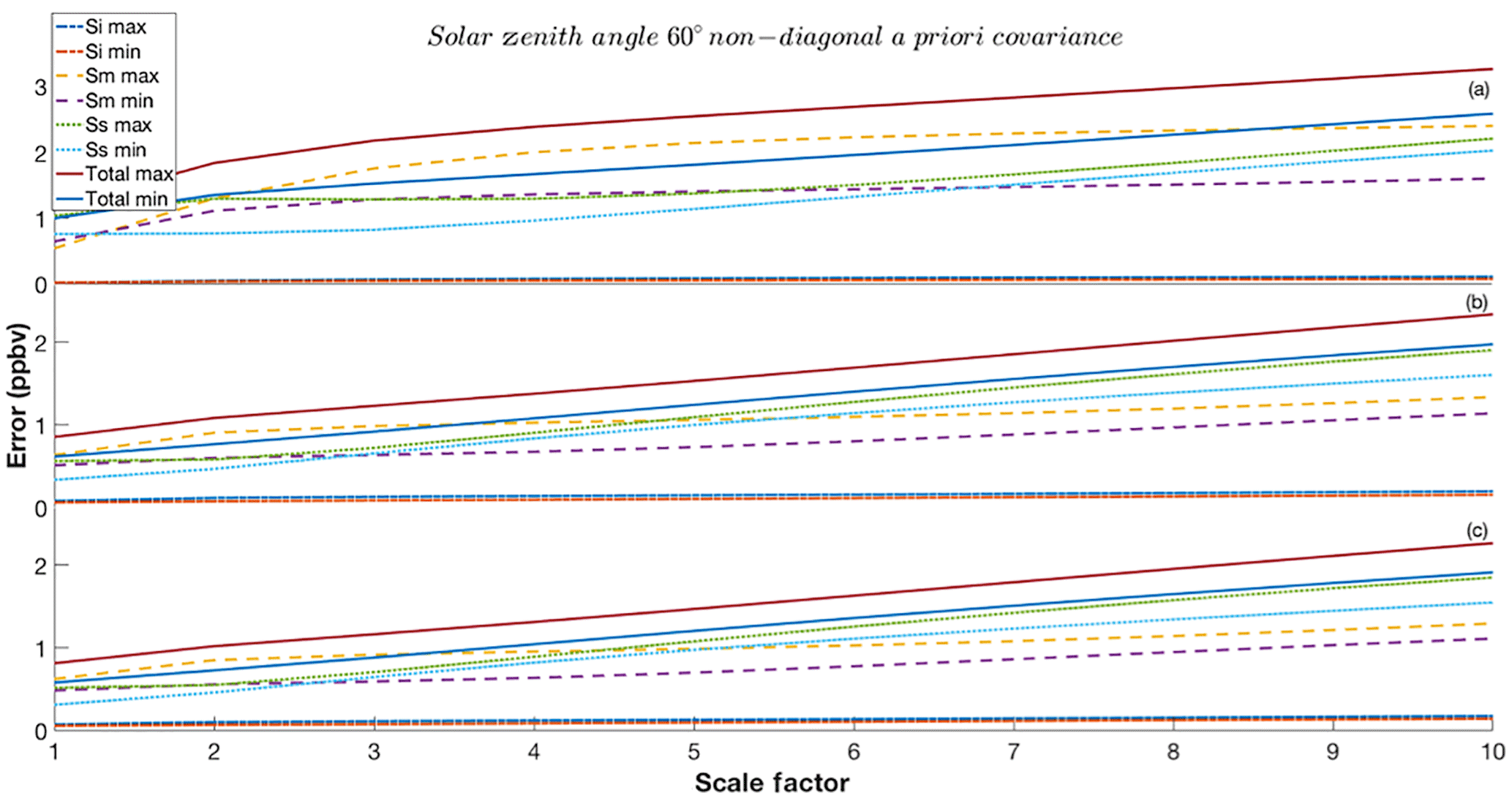
Figure A4Synthetic total column retrieval errors retrieval for scenarios outlined in Table 3, based on Eqs. (8), (9), (10) and (16). The maximum and minimum values (based on maximum and minimum SNR) for interference, measurement and smoothing error are shown, in addition to the total error: panel (a) indicates scenario 3, panel (b) indicates scenario 6 and panel (c) indicates scenario 9.
EM, YY, TM and JPM conceived and designed the experiments; EM performed the experiments, analysed the data and wrote the paper.
The authors declare that they have no conflict of interest.
This research was partially funded by NIES GOSAT-2 Project, in combination
with the first author's PhD grant from the National Centre for Earth
Observation (NCEO) through the Natural Environment Research Council (NERC)
based in the UK (award number 157550). We would also like to acknowledge Anu Dudhia at Oxford University for the ORFM and JAXA/NIES/MOE for
GOSAT-TANSO-FTS data.
Edited by: Piet Stammes
Reviewed by: Haili Hu and one anonymous referee
Aydin, M., Verhulst, K. R., Saltzman, E. S., Battle, M. O., Montzka, S. A., Blake, D. R., Tang, Q., and Prather, M. J.: Recent decreases in fossil-fuel emissions of ethane and methane derived from firn air, Nature, 476, 198–201, https://doi.org/10.1038/nature10352, 2011.
Bovensmann, H., Burrows, J. P., Buchwitz, M., Frerick, J., Noël, S., Rozanov, V. V, Chance, K. V., and Goede, A. P. H.: SCIAMACHY: Mission Objectives and Measurement Modes, J. Atmos. Sci., 56, 127–150, https://doi.org/10.1175/1520-0469(1999)056<0127:SMOAMM>2.0.CO;2, 1999.
Brown, L. R., Sung, K., Benner, D. C., Devi, V. M., Boudon, V., Gabard, T., Wenger, C., Campargue, A., Leshchishina, O., Kassi, S., Mondelain, D., Wang, L., Daumont, L., Régalia, L., Rey, M., Thomas, X., Tyuterev, V. G., Lyulin, O. M., Nikitin, A. V, Niederer, H. M., Albert, S., Bauerecker, S., Quack, M., O'Brien, J. J., Gordon, I. E., Rothman, L. S., Sasada, H., Coustenis, A., Smith, M. A. H., Carrington, T., Wang, X. G., Mantz, A. W., and Spickler, P. T.: Methane line parameters in the HITRAN2012 database, J. Quant. Spectrosc. Ra., 130, 201–219, https://doi.org/10.1016/j.jqsrt.2013.06.020, 2013.
Buzan, E. M., Beale, C. A., Boone, C. D., and Bernath, P. F.: Global stratospheric measurements of the isotopologues of methane from the Atmospheric Chemistry Experiment Fourier transform spectrometer, Atmos. Meas. Tech., 9, 1095–1111, https://doi.org/10.5194/amt-9-1095-2016, 2016.
Ceccherini, S. and Ridolfi, M.: Technical Note: Variance-covariance matrix and averaging kernels for the Levenberg-Marquardt solution of the retrieval of atmospheric vertical profiles, Atmos. Chem. Phys., 10, 3131–3139, https://doi.org/10.5194/acp-10-3131-2010, 2010.
Craig, H.: Isotopic standards for carbon and oxygen and correction factors for mass-spectrometric analysis of carbon dioxide, Geochim. Cosmochim. Ac., 12, 133–149, https://doi.org/10.1016/0016-7037(57)90024-8, 1957.
Dudhia, A.: The Reference Forward Model (RFM), J. Quant. Spectrosc. Ra., 186, 243–253, https://doi.org/10.1016/j.jqsrt.2016.06.018, 2017.
Eguchi, N., Saito, R., Saeki, T., Nakatsuka, Y., Belikov, D., and Maksyutov, S.: A priori covariance estimation for CO2 and CH4 retrievals, J. Geophys. Res., 115, D10215, https://doi.org/10.1029/2009JD013269, 2010.
Etiope, G.: Natural emissions of methane from geological seepage in Europe, Atmos. Environ., 43, 1430–1443, https://doi.org/10.1016/j.atmosenv.2008.03.014, 2009.
Fisher, R. E., France, J. L., Lowry, D., Lanoisellé, M., Brownlow, R., Pyle, J. A., Cain, M., Warwick, N., Skiba, U. M., Drewer, J., Dinsmore, K. J., Leeson, S. R., Bauguitte, S. J.-B., Wellpott, A., O'Shea, S. J., Allen, G., Gallagher, M. W., Pitt, J., Percival, C. J., Bower, K., George, C., Hayman, G. D., Aalto, T., Lohila, A., Aurela, M., Laurila, T., Crill, P. M., McCalley, C. K., and Nisbet, E. G.: Measurement of the 13 C isotopic signature of methane emissions from northern European wetlands, Global Biogeochem. Cy., 31, 605–623, https://doi.org/10.1002/2016GB005504, 2017.
Frankenberg, C., Aben, I., Bergamaschi, P., Dlugokencky, E. J., van Hees, R., Houweling, S., van der Meer, P., Snel, R., and Tol, P.: Global column-averaged methane mixing ratios from 2003 to 2009 as derived from SCIAMACHY: Trends and variability, J. Geophys. Res., 116, D04302, https://doi.org/10.1029/2010JD014849, 2011.
Frankenberg, C., Hasekamp, O., O'Dell, C., Sanghavi, S., Butz, A., and Worden, J.: Aerosol information content analysis of multi-angle high spectral resolution measurements and its benefit for high accuracy greenhouse gas retrievals, Atmos. Meas. Tech., 5, 1809–1821, https://doi.org/10.5194/amt-5-1809-2012, 2012.
GOSAT-2 Project Team: GOSAT-2 Project Site – About GOSAT-2, NIES, available at: http://www.gosat-2.nies.go.jp/about/spacecraft_and_instruments/, last access: 7 December 2017.
Heimann, M.: Enigma of the recent methane budget, Nature, 476, 157–158, https://doi.org/10.1029/2009GL039780, 2011.
Herbin, H., Labonnote, L. C., and Dubuisson, P.: Multispectral information from TANSO-FTS instrument – Part 1: Application to greenhouse gases (CO2 and CH4) in clear sky conditions, Atmos. Meas. Tech., 6, 3301–3311, https://doi.org/10.5194/amt-6-3301-2013, 2013.
Hu, H., Hasekamp, O., Butz, A., Galli, A., Landgraf, J., Aan de Brugh, J., Borsdorff, T., Scheepmaker, R., and Aben, I.: The operational methane retrieval algorithm for TROPOMI, Atmos. Meas. Tech., 9, 5423–5440, https://doi.org/10.5194/amt-9-5423-2016, 2016.
Illingworth, S. M., Allen, G., Newman, S., Vance, A., Marenco, F., Harlow, R. C., Taylor, J., Moore, D. P., and Remedios, J. J.: Atmospheric composition and thermodynamic retrievals from the ARIES airborne FTS system – Part 1: Technical aspects and simulated capability, Atmos. Meas. Tech., 7, 1133–1150, https://doi.org/10.5194/amt-7-1133-2014, 2014.
IPCC: Fifth Assessment Report – Impacts, Adaptation and Vulnerability, available at: http://www.ipcc.ch/report/ar5/wg2/ (last access: 12 June 2017), 2014.
Kai, F. M., Tyler, S. C., Randerson, J. T., and Blake, D. R.: Reduced methane growth rate explained by decreased Northern Hemisphere microbial sources, Nature, 476, 194–197, https://doi.org/10.1038/nature10259, 2011.
Khalil, M. A. K. and Rasmussen, R. A.: Global emissions of methane during the last several centuries, Chemosphere, 29, 833–842, https://doi.org/10.1016/0045-6535(94)90156-2, 1994.
Kirschke, S., Bousquet, P., Ciais, P., Saunois, M., Canadell, J. G., Dlugokencky, E. J., Bergamaschi, P., Bergmann, D., Blake, D. R., Bruhwiler, L., Cameron-Smith, P., Castaldi, S., Chevallier, F., Feng, L., Fraser, A., Heimann, M., Hodson, E. L., Houweling, S., Josse, B., Fraser, P. J., Krummel, P. B., Lamarque, J. F., Langenfelds, R. L., Le Quéré, C., Naik, V., O'doherty, S., Palmer, P. I., Pison, I., Plummer, D., Poulter, B., Prinn, R. G., Rigby, M., Ringeval, B., Santini, M., Schmidt, M., Shindell, D. T., Simpson, I. J., Spahni, R., Steele, L. P., Strode, S. A., Sudo, K., Szopa, S., Van Der Werf, G. R., Voulgarakis, A., Van Weele, M., Weiss, R. F., Williams, J. E., and Zeng, G.: Three decades of global methane sources and sinks, Nat. Geosci., 6, 813–823, https://doi.org/10.1038/ngeo1955, 2013.
Kuai, L., Natraj, V., Shia, R.-L., Miller, C., and Yung, Y. L.: Channel selection using information content analysis: A case study of CO2 retrieval from near infrared measurements, J. Quant. Spectrosc. Ra., 111, 1296–1304, https://doi.org/10.1016/j.jqsrt.2010.02.011, 2010.
Kuze, A., Suto, H., Nakajima, M., and Hamazaki, T.: Thermal and near infrared sensor for carbon observation Fourier-transform spectrometer on the Greenhouse Gases Observing Satellite for greenhouse gases monitoring, Appl. Optics, 48, 6716, https://doi.org/10.1364/AO.48.006716, 2009.
Levin, I., Bergamaschi, P., Don, H., and Trapp, D.: Stable isotopic signature of methane from major sources in Germany, Chemosphere, 26, 161–177, https://doi.org/10.1016/0045-6535(93)90419-6, 1993.
Lyulin, O. M., Kassi, S., Sung, K., Brown, L. R., and Campargue, A.: Determination of the low energy values of 13CH4 transitions in the 2ν3 region near 1.66 µm from absorption spectra at 296 and 81 K, J. Mol. Spectrosc., 261, 91–100, https://doi.org/10.1016/j.jms.2010.03.008, 2010.
Nisbet, E. G., Dlugokencky, E. J., Manning, M. R., Lowry, D., Fisher, R. E., France, J. L., Michel, S. E., Miller, J. B., White, J. W. C., Vaughn, B., Bousquet, P., Pyle, J. A., Warwick, N. J., Cain, M., Brownlow, R., Zazzeri, G., Lanoisellé, M., Manning, A. C., Gloor, E., Worthy, D. E. J., Brunke, E.-G., Labuschagne, C., Wolff, E. W., and Ganesan, A. L.: Rising atmospheric methane: 2007–2014 growth and isotopic shift, Global Biogeochem. Cy., 30, 1356–1370, https://doi.org/10.1002/2016GB005406, 2016.
Parker, R., Boesch, H., Cogan, A., Fraser, A., Feng, L., Palmer, P. I., Messerschmidt, J., Deutscher, N., Griffith, D. W. T., Notholt, J., Wennberg, P. O., and Wunch, D.: Methane observations from the Greenhouse Gases Observing SATellite: Comparison to ground-based TCCON data and model calculations, Geophys. Res. Lett., 38, L15807, https://doi.org/10.1029/2011GL047871, 2011.
Parker, R. J., Boesch, H., Byckling, K., Webb, A. J., Palmer, P. I., Feng, L., Bergamaschi, P., Chevallier, F., Notholt, J., Deutscher, N., Warneke, T., Hase, F., Sussmann, R., Kawakami, S., Kivi, R., Griffith, D. W. T., and Velazco, V.: Assessing 5 years of GOSAT Proxy XCH4 data and associated uncertainties, Atmos. Meas. Tech., 8, 4785–4801, https://doi.org/10.5194/amt-8-4785-2015, 2015.
Reuter, M., Bovensmann, H., Buchwitz, M., Burrows, J. P., Deutscher, N. M., Heymann, J., Rozanov, A., Schneising, O., Suto, H., Toon, G. C., and Warneke, T.: On the potential of the 2041–2047 nm spectral region for remote sensing of atmospheric CO2 isotopologues, J. Quant. Spectrosc. Ra., 113, 2009–2017, https://doi.org/10.1016/j.jqsrt.2012.07.013, 2012.
Rigby, M., Manning, A. J., and Prinn, R. G.: The value of high-frequency, high-precision methane isotopologue measurements for source and sink estimation, J. Geophys. Res.-Atmos., 117, D12312, https://doi.org/10.1029/2011JD017384, 2012.
Röckmann, T., Brass, M., Borchers, R., and Engel, A.: The isotopic composition of methane in the stratosphere: high-altitude balloon sample measurements, Atmos. Chem. Phys., 11, 13287–13304, https://doi.org/10.5194/acp-11-13287-2011, 2011.
Rodgers, C. D.: Inverse Methods for Atmospheric Sounding – Theory and Practice, World Scientific, Singapore, 2000.
Rothman, L. S., Gordon, I. E., Barbe, A., Benner, D. C., Bernath, P. F., Birk, M., Boudon, V., Brown, L. R., Campargue, A., Champion, J.-P., Chance, K., Coudert, L. H., Dana, V., Devi, V. M., Fally, S., Flaud, J.-M., Gamache, R. R., Goldman, A., Jacquemart, D., Kleiner, I., Lacome, N., Lafferty, W. J., Mandin, J.-Y., Massie, S. T., Mikhailenko, S. N., Miller, C. E., Moazzen-Ahmadi, N., Naumenko, O. V., Nikitin, A. V., Orphal, J., Perevalov, V. I., Perrin, A., Predoi-Cross, A., Rinsland, C. P., Rotger, M., Šimečková, M., Smith, M. A. H., Sung, K., Tashkun, S. A., Tennyson, J., Toth, R. A., Vandaele, A. C., and Vander Auwera, J.: The HITRAN 2008 molecular spectroscopic database, J. Quant. Spectrosc. Ra., 110, 533–572, https://doi.org/10.1016/j.jqsrt.2009.02.013, 2009.
Rothman, L. S., Gordon, I. E., Babikov, Y., Barbe, A., Chris Benner, D., Bernath, P. F., Birk, M., Bizzocchi, L., Boudon, V., Brown, L. R., Campargue, A., Chance, K., Cohen, E. A., Coudert, L. H., Devi, V. M., Drouin, B. J., Fayt, A., Flaud, J. M., Gamache, R. R., Harrison, J. J., Hartmann, J. M., Hill, C., Hodges, J. T., Jacquemart, D., Jolly, A., Lamouroux, J., Le Roy, R. J., Li, G., Long, D. A., Lyulin, O. M., Mackie, C. J., Massie, S. T., Mikhailenko, S., Müller, H. S. P., Naumenko, O. V., Nikitin, A. V., Orphal, J., Perevalov, V., Perrin, A., Polovtseva, E. R., Richard, C., Smith, M. A. H., Starikova, E., Sung, K., Tashkun, S., Tennyson, J., Toon, G. C., Tyuterev, V. G., and Wagner, G.: The HITRAN2012 molecular spectroscopic database, J. Quant. Spectrosc. Ra., 130, 4–50, https://doi.org/10.1016/j.jqsrt.2013.07.002, 2013.
Saeki, T., Saito, R., Belikov, D., and Maksyutov, S.: Global high-resolution simulations of CO2 and CH4 using a NIES transport model to produce a priori concentrations for use in satellite data retrievals, Geosci. Model Dev., 6, 81–100, https://doi.org/10.5194/gmd-6-81-2013, 2013.
Schaefer, H., Fletcher, S. E. M., Veidt, C., Lassey, K. R., Brailsford, G. W., Bromley, T. M., Dlugokencky, E. J., Michel, S. E., Miller, J. B., Levin, I., Lowe, D. C., Martin, R. J., Vaughn, B. H., and White, J. W. C.: A 21st-century shift from fossil-fuel to biogenic methane emissions indicated by 13CH4, Science, 352, 80–84, https://doi.org/10.1126/science.aad2705, 2016.
Schepers, D., Guerlet, S., Butz, A., Landgraf, J., Frankenberg, C., Hasekamp, O., Blavier, J. F., Deutscher, N. M., Griffith, D. W. T., Hase, F., Kyro, E., Morino, I., Sherlock, V., Sussmann, R., and Aben, I.: Methane retrievals from Greenhouse Gases Observing Satellite (GOSAT) shortwave infrared measurements: Performance comparison of proxy and physics retrieval algorithms, J. Geophys. Res.-Atmos., 117, D10307, https://doi.org/10.1029/2012JD017549, 2012.
Schwietzke, S., Sherwood, O. A., Bruhwiler, L. M. P., Miller, J. B., Etiope, G., Dlugokencky, E. J., Michel, S. E., Arling, V. A., Vaughn, B. H., White, J. W. C., and Tans, P. P.: Upward revision of global fossil fuel methane emissions based on isotope database, Nature, 538, 88–91, https://doi.org/10.1038/nature19797, 2016.
Sherwood, O., Schwietzke, S., Arling, V., and Etiope, G.: Global Inventory of Fossil and Non-fossil Methane δ13C Source Signature Measurements for Improved Atmospheric Modeling, NOAA, https://doi.org/10.15138/G37P4D, 2016.
Takagi, H., Houweling, S., Andres, R. J., Belikov, D., Bril, A., Boesch, H., Butz, A., Guerlet, S., Hasekamp, O., Maksyutov, S., Morino, I., Oda, T., O'Dell, C. W., Oshchepkov, S., Parker, R., Saito, M., Uchino, O., Yokota, T., Yoshida, Y., and Valsala, V.: Influence of differences in current GOSAT XCO2 retrievals on surface flux estimation, Geophys. Res. Lett., 41, 2598–2605, https://doi.org/10.1002/2013GL059174, 2014.
Thuillier, G., Hersé, M., Labs, D., Foujols, T., Peetermans, W., Gillotay, D., Simon, P. C., and Mandel, H.: The solar spectral irradiance from 200 to 2400 nm as measured by the SOLSPEC spectrometer from the ATLAS and EURECA missions, Sol. Phys., 214, 1–22, https://doi.org/10.1023/A:1024048429145, 2003.
Whiticar, M. J.: Carbon and hydrogen isotope systematics of bacterial formation and oxidation of methane, Chem. Geol., 161, 291–314, https://doi.org/10.1016/S0009-2541(99)00092-3, 1999.
Worden, J., Liu, X., Bowman, K., Chance, K., Beer, R., Eldering, A., Gunson, M., and Worden, H.: Improved tropospheric ozone profile retrievals using OMI and TES radiances, Geophys. Res. Lett., 34, L01809, https://doi.org/10.1029/2006GL027806, 2007.
Wuebbles, D. and Hayhoe, K.: Atmospheric methane and global change, Earth-Sci. Rev., 57, 177–210, https://doi.org/10.1016/S0012-8252(01)00062-9, 2002.
Wunch, D., Toon, G. C., Blavier, J.-F. L., Washenfelder, R. A., Notholt, J., Connor, B. J., Griffith, D. W. T., Sherlock, V., and Wennberg, P. O.: The Total Carbon Column Observing Network, Philos. T. Roy. Soc. A, 369, 2087–2112, https://doi.org/10.1098/rsta.2010.0240, 2011.
Yoshida, Y., Ota, Y., Eguchi, N., Kikuchi, N., Nobuta, K., Tran, H., Morino, I., and Yokota, T.: Retrieval algorithm for CO2 and CH4 column abundances from short-wavelength infrared spectral observations by the Greenhouse gases observing satellite, Atmos. Meas. Tech., 4, 717–734, https://doi.org/10.5194/amt-4-717-2011, 2011.
Yoshida, Y., Kikuchi, N., Morino, I., Uchino, O., Oshchepkov, S., Bril, A., Saeki, T., Schutgens, N., Toon, G. C., Wunch, D., Roehl, C. M., Wennberg, P. O., Griffith, D. W. T., Deutscher, N. M., Warneke, T., Notholt, J., Robinson, J., Sherlock, V., Connor, B., Rettinger, M., Sussmann, R., Ahonen, P., Heikkinen, P., Kyrö, E., Mendonca, J., Strong, K., Hase, F., Dohe, S., and Yokota, T.: Improvement of the retrieval algorithm for GOSAT SWIR XCO2 and XCH4 and their validation using TCCON data, Atmos. Meas. Tech., 6, 1533–1547, https://doi.org/10.5194/amt-6-1533-2013, 2013.
- Abstract
- Introduction
- Study requirements, models and instruments
- Information content analysis – theory
- A priori set up and covariance composition
- Sensitivities of bands 2 and 3
- Establishing information content
- Error analysis
- Potential validation methods
- Alternatives to a priori methods
- Conclusions and summary
- Code and data availability
- Appendix A
- Author contributions
- Competing interests
- Acknowledgements
- References