A simple biota removal algorithm for 35 GHz cloud radar measurements

Cloud radar reflectivity profiles can be an important measurement for the investigation of cloud vertical structure (CVS). However, extracting intended meteorological cloud content from the measurement often demands an effective technique or algorithm that can reduce error and observational uncertainties in the recorded data. In this work, a technique is proposed to identify and separate cloud and non-hydrometeor echoes using the radar Doppler spectral moments profile measurements. The point and volume target-based theoretical radar sensitivity curves are used for removing the receiver noise floor and identified radar echoes are scrutinized according to the signal decorrelation period. Here, it is hypothesized that cloud echoes are observed to be temporally more coherent and homogenous and have a longer correlation period than biota. That can be checked statistically using ∼ 4 s sliding mean and standard deviation value of reflectivity profiles. The above step helps in screen out clouds critically by filtering out the biota. The final important step strives for the retrieval of cloud height. The proposed algorithm potentially identifies cloud height solely through the systematic characterization of Z variability using the local atmospheric vertical structure knowledge besides to the theoretical, statistical and echo tracing tools. Thus, characterization of high-resolution cloud radar reflectivity profile measurements has been done with the theoretical echo sensitivity curves and observed echo statistics for the true cloud height tracking (TEST). TEST showed superior performance in screening out clouds and filtering out isolated insects. TEST constrained with polarimetric measurements was found to be more promising under high-density biota whereas TEST combined with linear depolarization ratio and spectral width perform potentially to filter out biota within the highly turbulent shallow cumulus clouds in the convective boundary layer (CBL). This TEST technique is promisingly simple in realization but powerful in performance due to the flexibility in constraining, identifying and filtering out the biota and screening out the true cloud content, especially the CBL clouds. Therefore, the TEST algorithm is superior for screening out the low-level clouds that are strongly linked to the rainmaking mechanism associated with the Indian Summer Monsoon region's CVS.

1 Introduction

Short-wavelength (millimetre-wave) Doppler radars are well known as cloud radars for their high sensitivity, which is required to sense the cloud droplets or ice crystals to infer cloud properties at high resolution (e.g. Lhermitte, 1987; Pazmany et al., 1994; Frisch et al., 1995; Kollias and Albrecht, 2000; Sassen et al., 1999; Hogan et al., 2005). The atmospheric radar echoes in the optically clear boundary layer are mainly from either Bragg scattering through refractive index irregularities due to turbulence in the atmosphere (wind profilers; e.g. Ecklund et al., 1988; Gossard, 1990) or particle scattering from hydrometeors and biota, which are airborne biological targets such as birds and insects, and waste plant materials such as dry leaves, pollen or dust (also known as “atmospheric plankton”, “atmospheric biota” or simply “insects”; Lhermitte, 1966; Clothiaux et al., 2000; Teschke et al., 2006). Although insects (hereafter biota) are probably the principal contaminants because of their size and dielectric constant, spiders, spiderwebs and other organic materials have been detected in the atmosphere through the use of nets and other means (Sekelsky et al., 1998). Furthermore, due to reduced scattering efficiency in the Mie region, cloud radar observations at 95 GHz are found to be less (∼ 5 dBZ) sensitive to biota than observations at 35 GHz (Khandwalla et al., 2003). Cloud radar signals frequently encounter these biota at an altitude within a couple of kilometres of Earth's surface, confined mostly to the atmospheric boundary layer (ABL). These echoes from the biota in the ABL have reflectivity values comparable to those from the clouds, and thus they contaminate and mask the true cloud returns (Luke et al., 2008). Though the nature of shallow clear-air radar echoes was first unknown, later these echoes over land in the convective boundary layer (CBL) were shown to be contaminated by particle scattering from biota rather than refractive index gradients (e.g. Gossard, 1990; Russell and Wilson, 1997). Importantly, clear-air echoes are a nuisance for radar-based studies on CBL clouds since they may contaminate the true cloud echo (e.g. Martner and Moran, 2001). However, these clear-air echoes can be advantageous in understanding and characterizing the CBL (e.g. Chandra et al., 2010, 2013; Geerts and Miao, 2015). But in order to utilize the potential purpose of cloud radar for studying clouds, one needs to identify and preserve the true cloud echoes from the biota contamination that is mostly confined within the ABL. The ABL shallow/low-level cumulus clouds are strongly linked to the rainmaking mechanism at the lower region of the cloud vertical structure (CVS) and are a key factor in predicting cloud feedback in a changing climate (Tiedtke, 1989; Bony et al., 2006; Teixeira et al., 2008) but their representation remain unresolved in large-scale mode-ling. This gives rise to the need for an unbiased and systematic observational study of shallow cumulus cloud to unravel its morphological as well as characteristic features. Therefore, the current work focuses on identifying and filtering biota echoes in order to significantly improve the quality of cloud radar data. This allows a better characterization of the tropical Indian Summer Monsoon's (ISM) CVS.

A review of previous studies shows that different techniques have been attempted to remove non-hydrometeor echoes, for example static techniques for the ground clutter (Harrison et al., 2014, 2000), return signal-level correction (Doviak and Zrnić, 1984; Torres and Zrnić, 1999; Nguyen et al., 2008), dynamic filtering (Steiner and Smith, 2002) and operational filtering (Alberoni et al., 2003; Meischner et al., 1997). The aforementioned studies were mostly confined to the use of single polarization radar. However, a new possibility has been developed using dual-polarization information to identify the non-meteorological clutter echoes (Zrnić and Ryzhkov, 1998; Mueller, 1983; Zhang et al., 2005). With the advent of Doppler spectral processing, it is possible to have an improved clutter mask (Bauer-Pfundstein and Görsdorf, 2007; Luke et al., 2008; Warde and Torres, 2009; Unal, 2009). As mentioned, one of the non-hydrometeor echoes is due to insects and airborne biota and these unwanted echoes are problematic for studies involving meteorological information such as wind measurements (Muller and Larkin, 1985) and true cloud returns (Martner and Moran, 2001). As a consequence, observations of biota were done using variable polarization and multiple-frequency radars operating initially in the centimetre wavelength (Hajovsky et al., 1966; Hardy et al., 1966; Mueller and Larkin, 1985). At millimetre-wavelength radar, Bauer-Pfundstein and Görsdorf (2007) showed effective linear depolarization ratio (LDR) filtering of biota while Khandwalla et al. (2003) and Luke et al. (2008) showed that dual-wavelength ratio filters are more effective than the LDR filters. Dual polarization also offers a wide variety of methods (e.g. Gourley et al., 2007; Hurtado and Nehorai, 2008; Unal, 2009; Chandrasekar et al., 2013). Fuzzy logic classification techniques for the identification and removal of spurious echoes from radar are also in use (e.g. Cho et al., 2006; Dufton and Collier, 2015; Chandra et al., 2013). From the above summary, it is therefore evident that most of the studies concentrate on either the polarimetric capabilities of radar or computationally intensive spectral processing of radar data to filter out echoes contaminated by non-hydrometeor targets. The importance of the work presented here lies in the development of an algorithm that uses solely high spatial and temporal resolution reflectivity measurements. These high spatial and temporal resolution (25 m and 1 s) measurements enable the characterization of irregular echoes associated with the spurious nature of radar returns due to biota. This method is simple and does not require spacious complex spectral data (and associated complicated analysis) or expensive advanced dual-polarimetric or dual-wavelength techniques.

Table 1 KaSPR specifications.

2 System, data and methodology

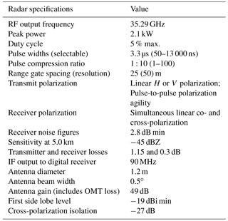
This investigation employs vertically oriented Doppler spectral moment profile observations of IITM's Ka-band scanning polarimetric radar (KaSPR) for the study of vertical cloud structure. Specifically, KaSPR employs an improved variation of the well-known linear frequency modulated (LFM) pulse compression technique. The KaSPR pulse compression technique is amplitude taper (window) (using a Tukey taper with 0.7 taper coefficient) on the transmitted LFM pulse and the compression is implemented in the digital signal processor system using a least mean squares filter (Mudukutore et al., 1998) to achieve much improved (lower) range side lobes compared to untapered LFM pulse compressed with a matched filter. Thus, KaSPR uses the 3.3 µs pulse length with 10X LFM chirp compression with effective range resolution of 50 m (i.e. compressed to 0.33 µs) and sampling in range (range gate spacing) at every 25 m with pulse reception frequency of 5 kHz. So, the radar data set used for this work has the range samples at every 25 m with first range gate altitude at 942 m a.g.l. KaSPR has been providing high-resolution (25 m and 1 s) resourceful measurements of cloud and precipitation at a tropical site (Mandhardev: 18.0429^∘ N, 73.8689^∘ E; 1.3 km a.m.s.l.) on a mobile platform since June 2013. Its other main technical features are given in Table 1. KaSPR possesses a sensitivity of $\sim -$60 (−45) dBZ at 1 (5) km and is therefore sensitive to the cloud droplet. According to T-matrix Rayleigh computations, a single 0.1 mm drop size of target at ∼ 35 GHz may have the reflectivity of $\sim -\mathrm{60}$ dBZ, whereas it needs near 63 drops each of 0.05 (0.01) mm size (or near 1 000 000 drops of 0.01 mm size) to give the same reflectivity. Furthermore, if there are 5000 (pulses per second) hits on the target in the radar scattering volume in 1 s, the mean of those 5000 samples at a range bin (height) will be affected by the mean characteristics of the target, such as composition, orientation, number density and kinematics associated with it. Therefore, it is safer to assume that the atmospheric or meteorological targets (in this case cloud particle) are distributive in nature and passive in the sense that their motion and/or orientation are in resonance with the kinematics of the background atmosphere. By comparison, birds and insects are point targets in nature and active in the sense that they can change their motion, direction and orientation within a few seconds. This leads to the irregular nature of intermittent or spurious radar returns that are characteristic of atmospheric biota due to the much smaller decorrelation time associated with them. This study utilizes the high-resolution profile of cloud radar reflectivity factor (Z) to construct the cloud vertical structures by filtering out the returns from the noise and biota.

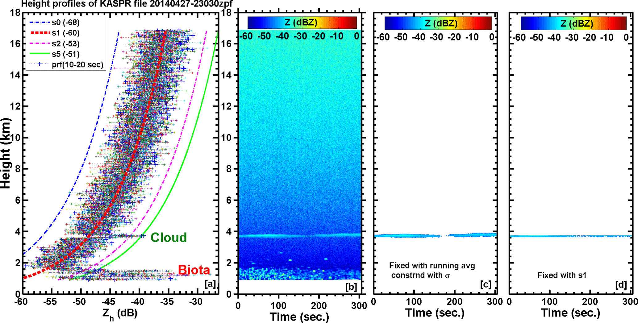
Figure 1 (a) Ten vertical-looking cloud-radar-measured sample reflectivity height profiles on 27 April 2014 during 23:03–23:08 UT. S0 to S5 are the theoretical noise-equivalent reflectivity curves with their respective threshold values in bracket. HTI plot of (b) the same reflectivity profile for the duration of 306 s (c) screened out reflectivity profile for the receiver noise floor and the biota (insects) using running average constrained with standard deviation (d) constrained with NER (S5).

Figure 1a represents the height profiles of zeroth moment (radar echo peak power) based Z on 27 April 2014 at 23:03 UT with various theoretical radar sensitivity (noise-equivalent reflectivity, NER) curves (S0–S5; the range profile correction with the start range sensitivity value of reflectivity, i.e. r²×Z_{start range}, where r is range or height and Z is reflectivity; e.g. for S1, Z is −60 dBZ). These different NER or sensitivity curves are utilized to qualify the observed radar returns that are indeed above the NER, the inherent radar receiver noise level. The receiver noise level is the inherent thermal noise associated with electronic components in the receiver chain, as well as other sources that are taken into account through the noise figure (Table 1), and it remains approximately constant over the length of the pulse returns. However, range correction is intuitive in the radar equation due to the decrease in echo signal strength with increasing height (for vertical orientation). In order to determine the noise range in every range bin, S0 to S5 are computed and overlaid on Z. This allows for identification and characterization of the signal that overlays the background system noise level. As discussed earlier, the signal at any level may have contributions due to either volumetric meteorological cloud particulates or strong non-meteorological/non-hydrometeor point targets (e.g. biota). In Fig. 1a the echoes at ∼ 3.7 km and below 2 km can be marked as cloud and biota, respectively, as they exceed the profile S5. The noise variations around 15 dB are mostly confined between S0 and S2 with S1 as mean NER. Contrasting echo texture associated with the cloud and atmospheric biota is evident from the height–time–intensity (HTI) plot of Z in Fig. 1b. This is a weak cloud case with reflectivity ∼ −38 dBZ at ∼ 3.7 km altitude with the presence of intermittent, non-homogeneous echo texture from the biota below 2.7 km altitude. A similarly weak cloud case of $-\mathrm{38}\pm \mathrm{2}$ dBZ at 5.4 km altitude is confirmed as cloud with the sharp increase in relative humidity of ∼ 80 % at that altitude by collocated radiosonde (GPS–RS) measurements but is not shown here (see Fig. A2). Biota echoes are observed to be confined most densely below 1.7 km and fall in the reflectivity range of −50 to −20 dBZ. The observed standard deviation (SD) is always more than 2 dBZ and can indirectly infer the decorrelation period of ∼ 4–5 s (returns due to biota are observed to vanish at an interval of ∼ 3–8 s; see the lower part of the HTI plot). In the decorrelation period, it is hypothesized here that the running mean and SD of ∼ 4 s sliding window reflectivity profiles work in identifying all non-hydrometeor returns. Furthermore, the time coherence of radar returns at every range sample can be checked every 4 s as a window period to infer the echo power decorrelation time or degree of coherence period associated with biota returns based on the SD of Z value. Two sensitivity (S1 and S5) tests have been performed on Z profile to quantify noise floor, biota and the meteorological cloud returns. All the tests have been affected by the presence of non-meteorological echo due to biota even though these are mostly present in the ABL. Reflectivity values associated with the cloud boundaries are very faint and fall within or close to system noise floor by 2–5 dBZ. The profile S5 seems to be better at screening out the cloud echoes 10 dBZ above the radar receiver mean noise floor, but this can eliminate a significant portion of the weakest reflectivity area at the cloud edge (Fig. 1d). Apart from clouds, biota also show higher reflectivity values than S5. Figure 1d is similar to Fig. 1b except it is completely screened out for cloud by applying the typical threshold of radar system sensitivity profiles S1 and S5. In addition to this, in the case of Fig. 1c, a contiguous set of four reflectivity profiles has been considered for computing running mean and SD. The method used to generate Fig. 1c is the main objective of this paper and is outlined by the flowchart in Fig. 6. This method will be explained below; Sect. 3 contains thorough information. In this case, insect reflectivity values are similar to those of the cloud but their altitude levels are significantly different. The contribution due to biota can therefore be removed by S5 curve thresholding, leaving the contribution due to clouds untouched (Fig. 1d). Thus, for the simultaneous presence of cloud and biota echoes at around same altitude this NER method fails to identify the contributions separately. This NER method also fails whenever sharp reflectivity changes occur, usually seen with cloud boundaries and edges. This issue therefore demands the development of a robust algorithm that explores the fundamental difference between cloud and biota returns so that it could be identified and separated out automatically.

In order to make the algorithm more robust for running it automatically, a close re-inspection of Fig. 1b shows that cloud returns are much more regular and near homogeneous when compared to biota returns, which appear to be spurious or intermittent in occurrence. Therefore, the NER criterion works reasonably well for the case of homogeneous, isolated stable cloud layers but its robustness is questionable whenever there are vigorous and quick changes associated with cloud edge and/or structure (explained in the discussion of clouds 1–2 in Fig. 5). An additional criterion makes the current algorithm robust for complete revival of cloud information from the Z observations by utilizing the decorrelation periods of biota (close to 3–5 s). During this time interval significant changes are not seen within the cloud. To explore this fact, in the next section the same weak low-level cloud case has been chosen to understand the coherence period associated with cloud and biota.

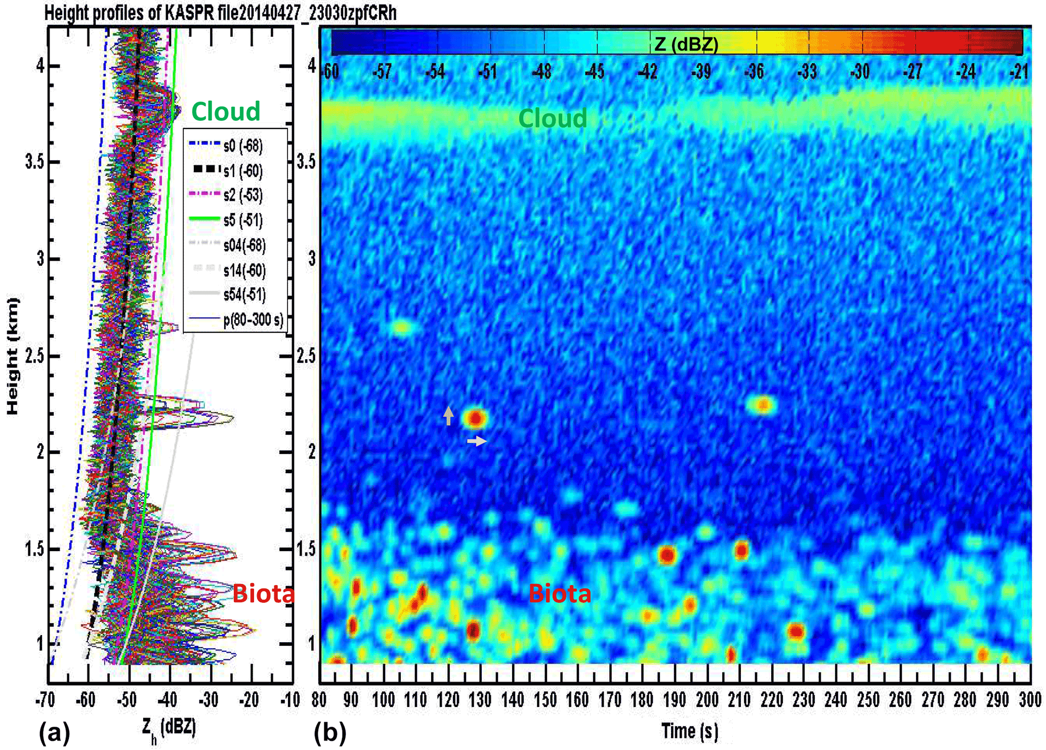
Figure 2 (a) Same as Fig. 1a but for 220 profiles. Extra NER curves, here in grey (S04, S14 and S54), are computed on the basis of the point target radar equation (i.e. r⁴×Z_{start range}, where r is range and Z is reflectivity; e.g. for S04, Z is −68 dBZ). (b) HTI plot of Z profiles. The smoothly varying homogeneous cloud layer is at altitudes of 3.5–3.8 km and sharp, rounded and spurious kinds of echoes below 2.7 km are due to biota.

3 Results and discussions

Figure 2 takes the same case as in Fig. 1 but confined below 4 km and 80–300 s (left panel). The added NER curves in grey (S04, S14 and S54; the range correction for the point clear-air target (confined below 3 km) with the start range sensitivity value of reflectivity, i.e. r⁴×Z_{start range}, where r is range and Z is reflectivity, for S14; e.g. Z is −60 dBZ). Figure 2 reveals three main type of radar signal region, namely (1) consistent radar returns characterized by the smooth and gradual change(s) associated with cloud particles (at ∼ 3.7 km height), (2) sharp (gradient) and spurious radar returns (at altitude below 2.7 km) due to point target(s) and (3) receiver noise floor. In order to locate these signal types easily, various sensitivity or NER (i.e. S0–S5) curves have been utilized. The second type of signal is associated with a characteristic point target (which has sharp reflectivity gradient feature due to the target's limited spatial as well as temporal spread associated with the radar scattering volume). The third type, noise floor (not radar echo but signal generated in the receiver chain of the radar), is seen to be confined mostly between S0 and S2. The right panel in Fig. 2 corresponds to the HTI plot, in which the echo texture pertinent to the abovementioned three echo types can be clearly visualized. The cloud echoes spread in the altitude region of approximately 300 m (3.6–3.9 km) with consistently smooth and gradual evolution with its weakest and/or broken structure during 165–190 s. In contrast to this the observed irregular point or rounded texture of biota echo spread is seen to be limited temporally around 3–7 s and spatially within two (four) range gates (range samples) size (i.e. < 100 m) with the strongest reflectivity at its centre. This indicates that 1 s temporal resolution might be good enough to see the biota as points or as rounded echo texture. When biota density is more in the lower altitude levels, it is difficult to clearly identify the boundary of one point target from another. Such a scenario, though rare, can lead to misidentification as clouds. The coexistence of cloud and transient high-density flocks of biota adds complexity, which becomes almost impossible to discriminate. However, this issue is observed to be rare and limited to the lowest altitudes only.

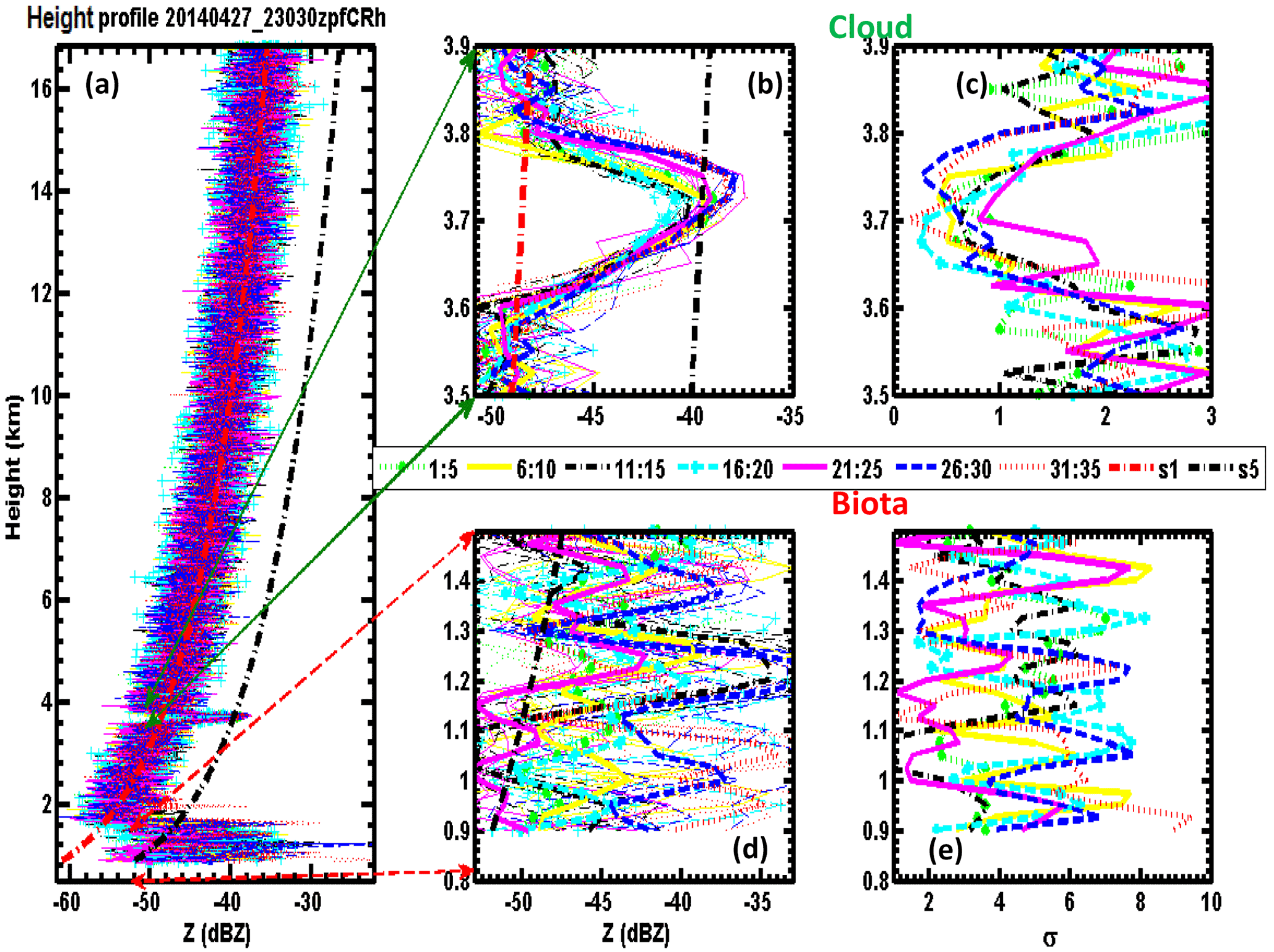
Figure 3 (a) Same as Fig. 1a but for 105 profiles. (b) Mean and (c) standard deviation of 15 profiles of Z pertinent to cloud height region (3.5–3.9 km) and (d) and (e) same as (b) and (c) but pertinent to biota height region (0.9–1.5 km).

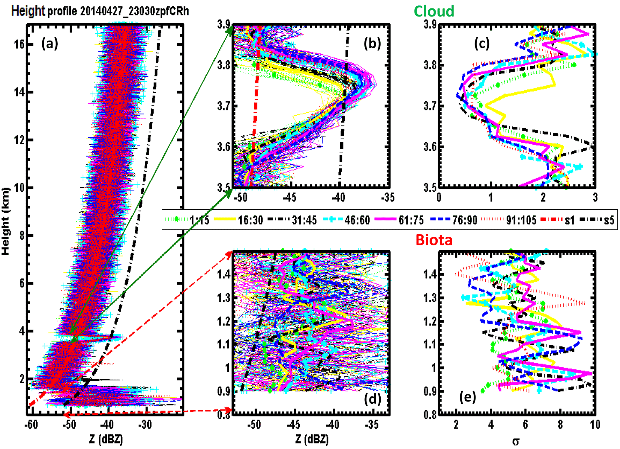
Figure 4 Same as Fig. 3 but for total duration 35 s; the mean and standard deviation profiles are for every 5 s interval.

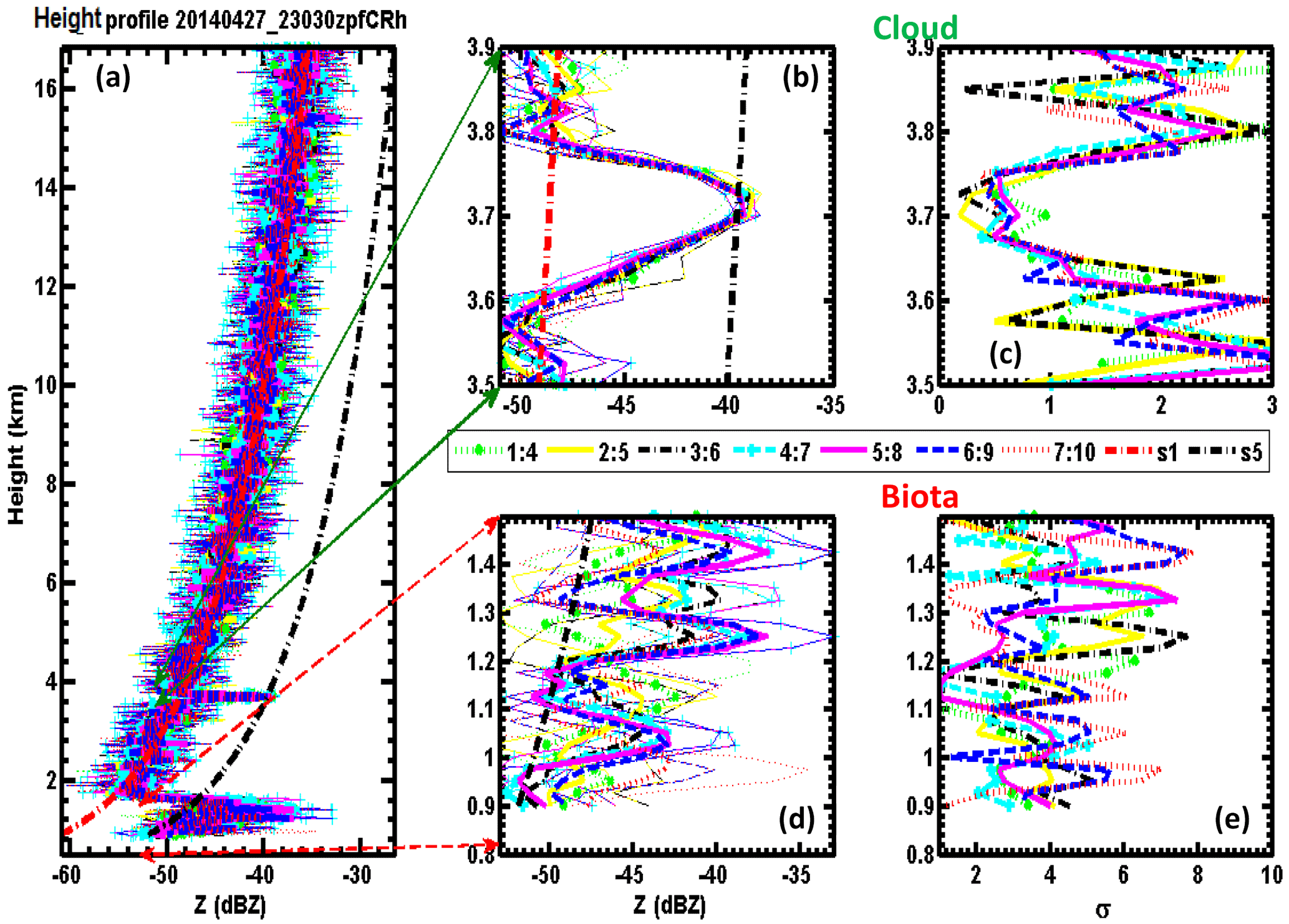
Figure 5 Same as Fig. 3 but for total duration 10 s; the mean and standard deviation profiles are for 4-point-moving average.

To investigate the similarities and contrasting features associated with various contributions to the cloud reflectivity profile, it is important to explore further the case of Fig. 1. Statistical echo coherence periods associated with three types (cloud, biota and noise) have been computed for their identification and separation. Both the cloud in the ∼ 3.7 km narrow region and biota returns below ∼ 1.5 km in Fig. 3 are evident above the maximum noise level. Both cloud and biota parts of the Z profiles are expanded to allow for review of the mean (Fig. 3b and d) and SD (σ; Fig. 3c and e) of Z for every set of consecutive 15 profiles. Figure 3b shows that the patterns of the seven mean cloud reflectivity profiles are organized and more consistent or correlated to one another during 105 s; this is in comparison to less organized reflectivity profiles due to biota that are much less consistent or correlated with one another in Fig. 3d. Moreover, the corresponding seven σ profiles show differences for cloud that are less than 1.5σ (Fig. 3c). By comparison, differences in profiles due to biota are more than 4.0σ most of the time (Fig. 3e). It is seen that the mean cloud reflectivity peak values gradually extend from 3.7 to 3.8 km, where the corresponding SD values are less than 1σ. In order to further test the minimum decorrelation time associated with cloud and biota, the averaging time is reduced to a set of five profiles (5 s) with the same data (see Fig. 4). In this case, Fig. 4c also depicts σ for all seven mean cloud reflectivity profiles below 1.5 dBZ with peak < 1σ. This shows that the volumetric distribution nature of cloud particles is statistically more homogeneous or show less dispersion. However, Z values associated with biota show random behaviour with significant dispersion > 1.5σ dBZ (Fig. 4e). This high dispersion in the Z values shows that the echo due to biota decorrelates quickly within ∼ 5 s time interval (see Fig. 4d–e). It is seen in Fig. 3 that for vertical levels from 0.9 km to 1.5, the sharp peaks in reflectivity profiles and strong dispersion of > 3σ dBZ are associated with the return from biota. This is attributed mostly to the observed intermittent point target nature of biota echoes plausibly due to the rambling or meandering motion of biota within the radar sampling volume. Moreover, the inherent radar system noise (random in nature) dispersion is observed between the cloud and biota (1.5–3.0σ dBZ). It is evident from the top panels of Fig. 3–4 that cloud reflectivity profiles show a relatively more consistent trend and correlation among the contiguous mean profiles computed from the set of 15 Z profiles than computed from the five profiles. This may be mainly due to the homogeneities or inhomogeneities associated with the manner in which the sample points are chosen from the data set. Therefore, in order to preserve the real time sequence of observations for the study of cloud evolution as well as to recover underlying smooth trends pertinent to natural clouds, a four-point moving or running average is applied on the time series of Z data instead of deriving a simple average. The 4 s moving average time is optimal for yielding the best cloud results (Fig. 5) by characterizing the cloud to biota echoes as coherent to incoherent property during the moving average period. By this four-point running average, biota echoes become incoherent due to their short decorrelation period (∼ 4 s), whereas those echoes decorrelating over longer periods indicate the presence of clouds. To understand the degree of dispersion, the absolute deviations in mean and median values also must be analysed along with σ. The mean absolute deviation is slightly smaller than σ, σ∕1.253, whereas the median absolute deviation is smallest, σ∕1.483. This work makes use of the statistical mean and σ but, by using the above relation, one can relate the present results with other central statistical tendencies of data distribution. Next, the filtering of noise and biota from the presence of cloud using the cloud radar reflectivity profile will be explored. The segregation has been carried out using theoretical radar echo sensitivity curves and statistically computed echo decorrelation periods and finally tracking the cloud echo peak to its adjacent sides until it is close to the S1 profile for the cloud height. The above set of tasks, theoretical echo sensitivity and observed echo-based statistics for cloud height tracking (TEST), is repetitively performed on the cloud radar Z measurements under an algorithm whose flowchart is in Fig. 6. The algorithm used in this work is named as TEST and can be summarized below:

1. Wherever the moving mean Z values in the profile are equal to or above the S5, this can be qualified as cloud or biota echo. This step ensures removal of the system noise floor.

2. Those altitude regions of the qualified echo are then further scrutinized to identify clouds using the minimum thickness of greater than 100 m (to strictly avoid biota that are found to extend less than two range gates, each of size 50 m) and mean standard deviation below 1.5σ dBZ.

3. In order to keep the identified cloud's structure intact, the identified cloud peak(s) are tracked back on either side (towards upper and bottom heights) up to around (preferably 1–2 dBZ) the mean noise profile S1.

4. Finally, the remnant isolated echo floor is not related to cloud but occurs due to the abrupt disconsolation at the subsequent running average by the restrictions of step 2. In order to remove those, the frequency count of Z profile has been constrained at those height levels where the Z frequency count falls below 5 % of total measurement.

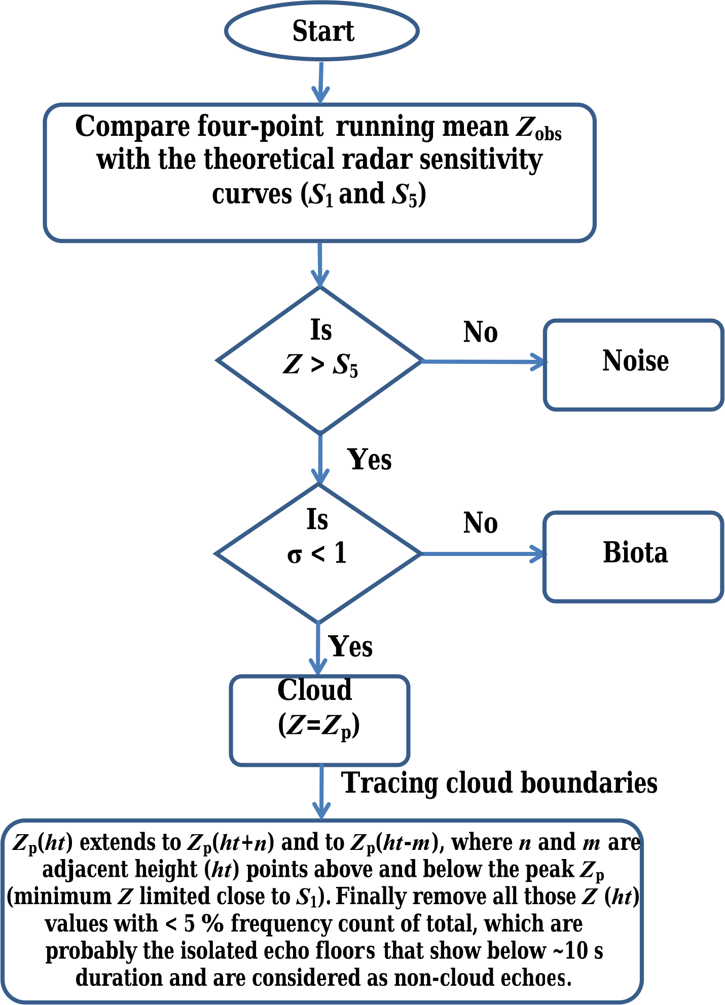
Figure 6 TEST algorithm flow chart that identifies and filters out the biota and noise echoes for screening out the cloud contributions with the Z measurements.

The first two steps ensure the identification and removal of non-hydrometeor contributions from the cloud radar reflectivity profile, which can then be used for inferring unbiased vertical cloud structure. However, these two steps are insufficient for recovering the weakly echoing cloud boundaries associated with the sharp reduction in cloud droplet size and concentrations. To have intact cloud height information (step 3), identified cloud echo peaks need to be backtracked along the either sides on the reflectivity profile until its value falls close to the mean noise floor for radar receiver. It is interesting to note that the cloud echo regions are always stronger and above the mean noise fluctuations, i.e. S1. Therefore on the left side of the curve, S0 to S1 always appear as a void region in the two-dimensional reflectivity plot wherever there are clouds present, no matter how weak or strong (just below 4 km in the left panel of Figs. 1 and 3). This causes sharp boundary gradients between cloud and noise in the vertical profiles of Z and hence the corresponding σ. This can be used as a visual criterion for detection of cloud.

Figure 7 is similar to Fig. 1 but it represents a multilayer pre-monsoon cloud system for the period 12:00–12:05 UT, 29 May 2014. Various labelled altitude regions (biota, noise and cloud) of the vertical reflectivity structure show typical mean features that can broadly classify the returns into cloud and non-cloud (biota and noise) portion. Furthermore, Fig. 7 shows the typical variety of cloud layers existing within the vertical structure of tropical cloud as well as morphological features pertinent to pre-monsoon thunderstorm activity. The cirrus layer at 12–14 km shows gradual structural change with peak reflectivity values of ∼ 5 dBZ. Here, the high reflectivity values contribute to form deep, single convective clouds by merging with the cloud layer that exists at lower heights.

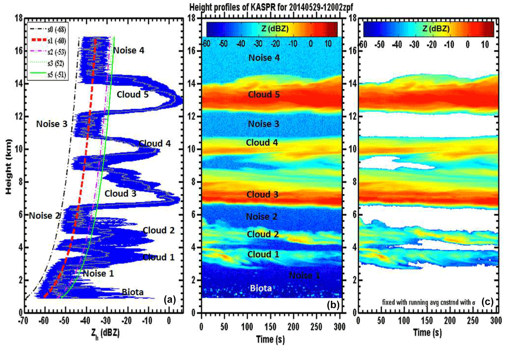
Figure 7 (a–c) Same as Fig. 1a–c but on 29 May 2014 during 12:00–12:05 UT for the duration of 306 s. Statistics correspond to the labels on the Z profile can be seen in Table 2.

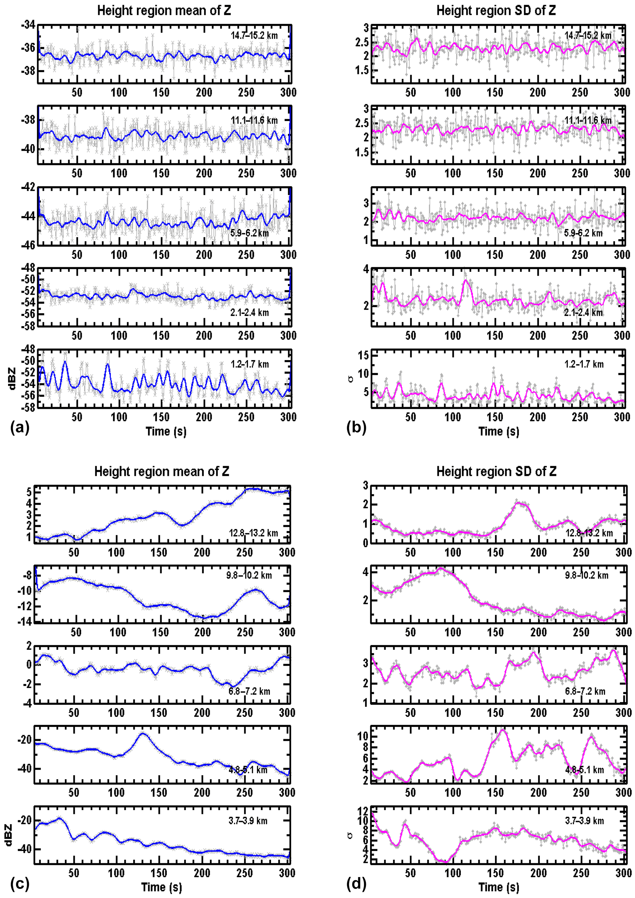
Figure 8 Time series of the mean and standard deviation (SD) of Z (a–b) for two biota and four noise floor regions as per Table 2. Bold solid lines are the five-point-running mean over the actual time series data (lines with symbol). (c–d) Same as (a–b) but for the cloud regions as per Table 2.

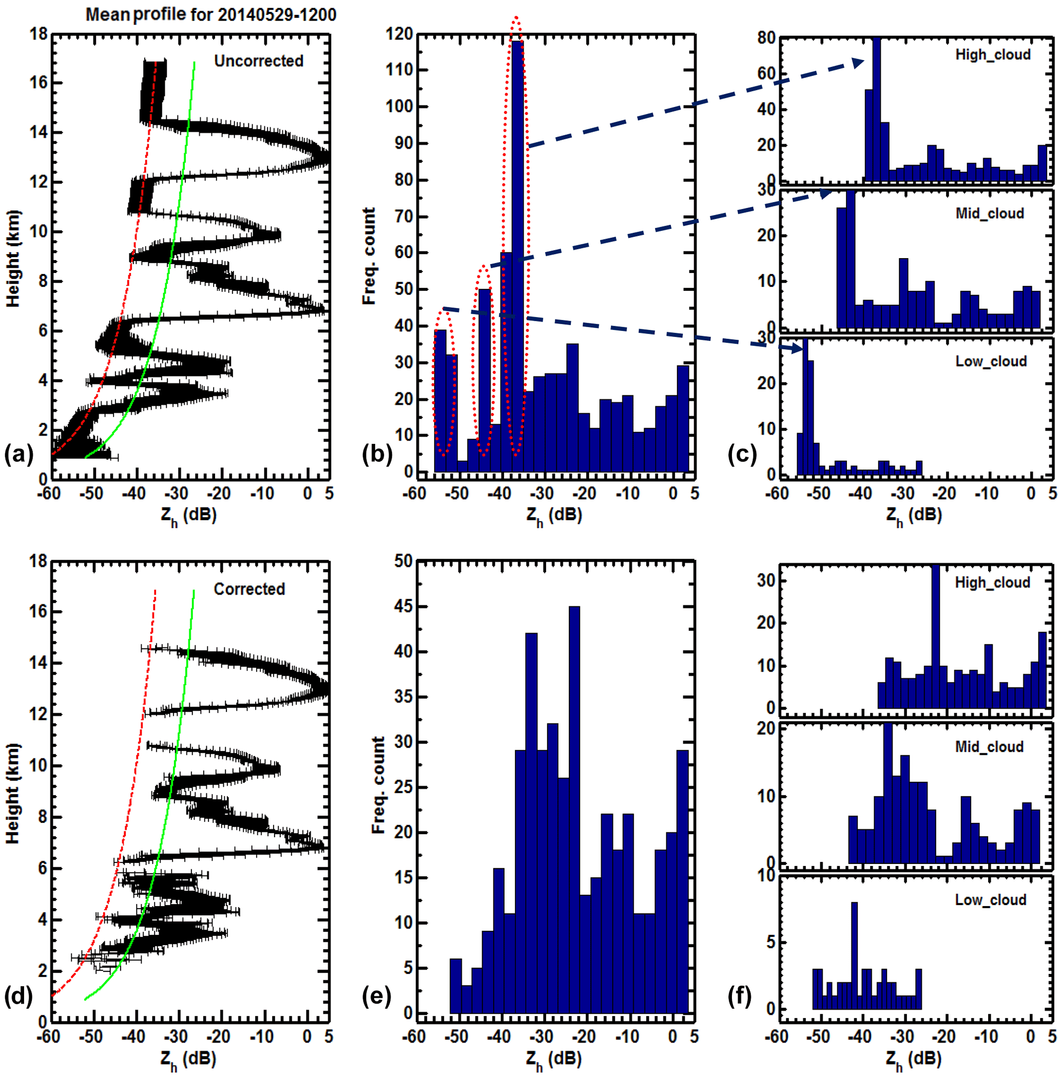
Figure 9 (a) Uncorrected mean reflectivity profile on 29 May 2014 during 12:00–12:05 UT, superimposed with curves S1 (dashed red line) and S5 (solid green line). (b) Histogram of whole uncorrected Z profile. (c) Three sub-panels of low (< 3.6 km), middle (3.6 km > = ht < 8.6 km) and high (> = 8.6 km) altitude regions. Each histogram peak in the three top right sub-panels is mapped onto the corresponding three peaks, indicated by dotted circles in panel (b). This shows that the noise clearly suppresses the meteorological information. (d) Same as Fig. 9a but corrected by filtering out noise and biota. (e) The correction applied to Z profile pops up the true meteorological cloud reflectivity distribution, which can be seen in panel (f) (same as c but for corrected Z).

Figure 8a and b reveal the reflectivity time series associated with the labelled non-cloud and cloud portion of Table 2, respectively. Noise and biota show maximum 2 dBZ fluctuations around the four-point-running mean reflectivity, whereas for biota the max fluctuation is 3–5 dBZ (bold solid line). It can be understood that noise values increase gradually with altitude with σ values ∼ 2.3 whereas sharp boundary gradients associated with biota and ragged shallow cloud regions (clouds 1 and 2 in Fig. 7) also show higher σ values > 3 dBZ. Stable or layered cloud regions (clouds 4 and 5 in Fig. 7) show significantly standard deviations below 2σ (dBZ). Further, it is interesting to examine the time series plots for the contrasting variations between the biota and noise and cloud regions with Fig. 8a and b. The range of dBZ variability is 4–10 dBZ for biota and 2–4 dBZ for noise and less than 1 dBZ for cloud within an interval of 5–10 s. The corresponding variability in SD is observed to be 4–10σ for biota, 1.5–3.5σ for noise and ∼ 1σ for cloud (< 1σ for cloud peak) except for weaker cloud regions. These statistical characteristics of all types of observed cloud echoes have been tabulated in Table 2.

Figure 9 demonstrates the application of the work presented here and illustrates the significant differences between the uncorrected (Fig. 9a–c) and corrected (Fig. 9d–f) reflectivity profiles. The peaks in frequency distribution of uncorrected cloud reflectivity profiles at just below −50 dBZ, between −50 and −40 and just above −40 dB are the predominant contributions from noise (Fig. 9b). These noise regions severely bias the corresponding histogram frequency distribution at three different altitude levels associated with Johnson's trimodal cloud distribution (Fig. 9c). In order to infer the distribution of cloud reflectivity values in the various altitude regions pertinent to trimodal CVS (Johnson et al., 1999), the observed vertical structure is subdivided into warm or low (< 3.6 km), mixed or middle (3.6 km ≥ altitude ≤ 8.6 km) and ice or high (> 8.6 km) phase and/or level clouds. The plots of uncorrected reflectivity distribution clearly show skewness towards lowest values of reflectivity (below −50, −40 and −30 dB for low, middle and high levels, respectively, seen in Fig. 9c). This is mainly due to the predominance of noise contribution, except for the low cloud regions, where the contribution of biota is also included. After applying the TEST algorithm the corrected reflectivity distribution peaks at −42, −35 and −22 dB for low, middle and high levels, respectively (Fig. 9f), reflecting the actual scenario of the cloud system. This method is simple and has the potential to bring out the statistically significant micro- and macro-physical characteristics from meteorological information (i.e. cloud) and hence help better characterize the CVS over a region.

Table 2 Statistical mean and standard deviation of cloud radar reflectivity corresponds to the selected height regions, which are labelled, on the Fig. 7.

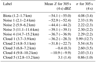
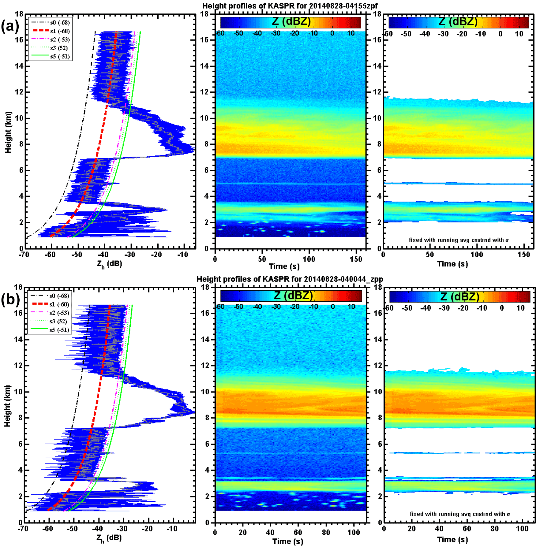
Figure 10 Same as Fig. 7 but for vertical-looking KaSPR measurements at 04:00 UT on 28 August 2014 using (a) FFT processing and (b) PP processing on 15 min prior observations. PP case will be used to evaluate the polarimetric algorithm performance.

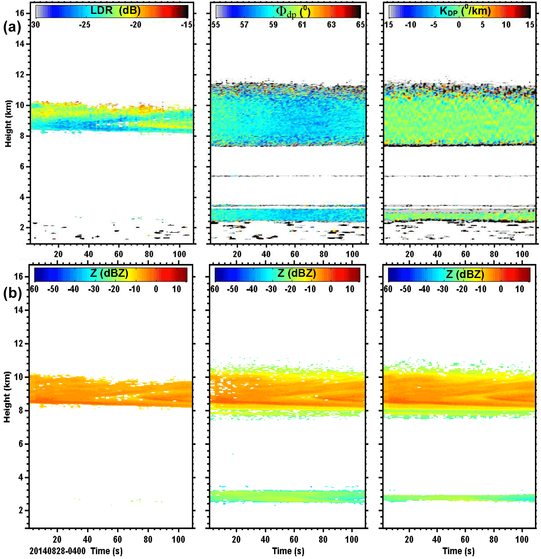
Figure 11 HTI plots of (a) LDR, Φ_dp and K_DP parameters pertinent to PP processed data of Fig. 10 and (b) biota-filtered reflectivity after applying corresponding polarimetric thresholds of the respective top panels.

In order to test the merit of the current algorithm for filtering out the non-hydrometeor contribution with Z profile, the parametric thresholds on pulse-pair (PP) processed Z and the polarimetric variable profiles of the cloud radar measurements have also been considered in place of the usual fast Fourier transformation (FFT) process. The FFT process is able to provide only the polarimetric parameter, i.e. LDR. Figure 10 is similar to Fig. 1, illustrating FFT (top) and PP (bottom) processed Z profiles on 28 August 2014; however, they are 15 min apart from one another (04:15 and 04:00 UT, respectively), which causes some dissimilarities in the observed three-layer cloud structure between the two plots (upper and lower panel). The minimum range of the noise floor in the Z profiles (2-D plot in the first panel) is seen to be greater for PP than FFT processing. The TEST algorithm performs in a similar way for both the FFT and PP processed Z profiles and is able to isolate the cloud structure as well as possible. Figure 11 further explores the polarimetric capability of the KaSPR to separate out the meteorological–hydrometeor contribution of Z by using critical thresholds on the PP-polarimetric measurements that correspond to Fig. 10b. Figure 11a stand for HTI plots of, three polarimetric parameters namely, LDR, Φ_dp and K_DP. Computation of LDR is inherently limited to the cross-polar isolation of the radar system that is −27 dB for KaSPR. Hence, high LDR values above −17 dB are mostly seen with biota and low LDR values below −17 dB are seen with cloud. Low to lower LDR values (i.e. <−17 to −25 dB) are strictly confined within the peak values of co-polar reflectivity (>−10 dB) of cloud altitude regions, ∼ 8–10 km. Except for the inherent limitations associated with LDR, these results are in agreement with earlier reported results (e.g. Bauer-Pfundstein and Görsdorf, 2007, and Khandwalla et al., 2003). The LDR, Φ_dp and K_DP threshold values are set below −17 dB, 56^∘ and −15^∘ km⁻¹, respectively, and can be used to filter out biota from the corresponding Z profiles that are shown in Fig. 11b. The thresholds used for Φ_dp and K_DP are subjective depending on the observed case for better filtering of biota. These polarimetric threshold methods are successful in filtering out the non-hydrometeor contributions, but they are bound to sacrifice the weaker portion of the cloud where polarimetric computations are not perfect. Thus, the polarimetric method is unable to preserve the weaker portions of the whole cloud regions, where the TEST method performs better (bottom right panel of Fig. 10). This further proves the efficiency of the proposed TEST method. TEST is implemented in the post-processing of high-resolution reflectivity measurements. The method developed here is far simpler and provides a superior solution to filtering out signal due to noise and biota and preserving cloud data in the form of pure hydrometeor reflectivity measurements which can be used to infer the true characteristics of clouds.

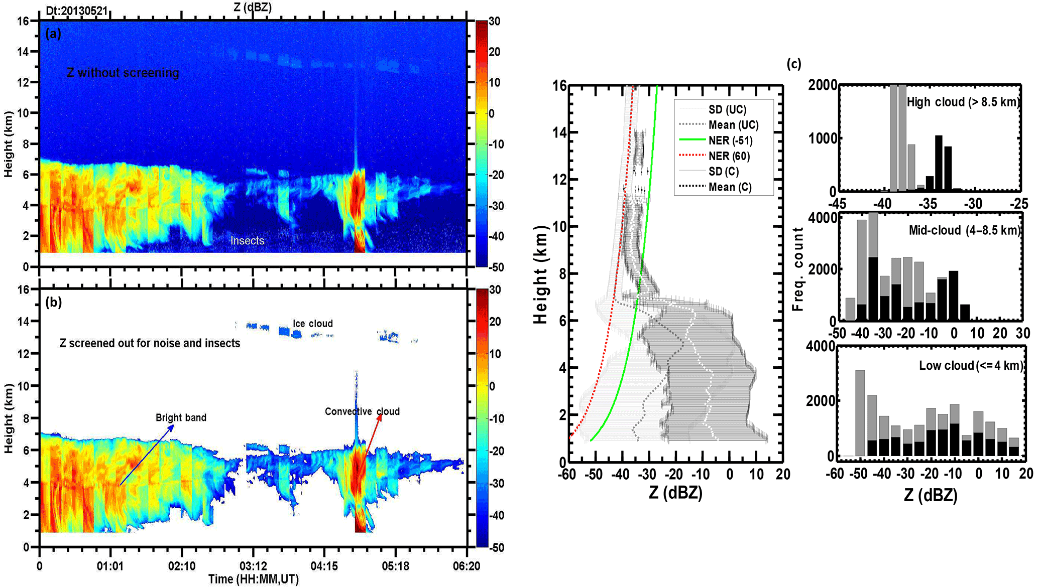
Figure 12 (a) Same as Fig. 7b (uncorrected) and (b) same as Fig. 7c (corrected) but integrated for duration of 00:00–06:30 UT taken at an interval of ∼ 15 min on 21 May 2013. (c) Merged form of Fig. 9a and d (line profiles) and Fig. 9c and f (histograms) using uncorrected and corrected Z data of (a) and (b) can be seen in the grey and black bars, respectively.

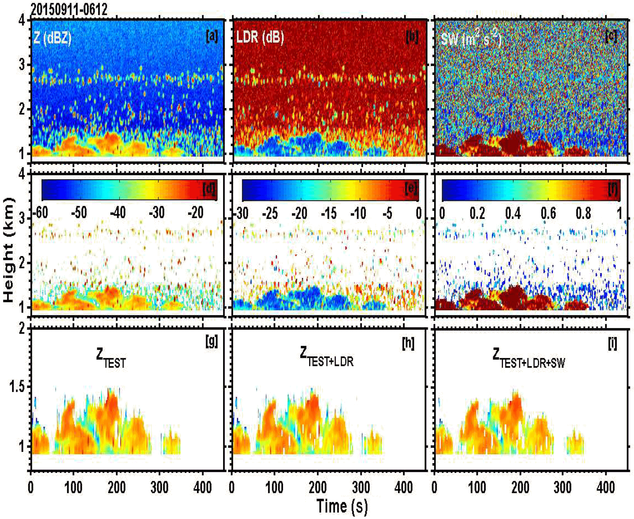
Figure 13 Cloud radar measurements of reflectivity (Z), LDR, spectral width (SW) with noise (a–c) and filtered out for noise using S5 curve (d–f), TEST algorithm screened output Z for clouds (g), (g) + biota filtering using LDR > −14 dB (h) and (h) + SW filter for biota using SW < 0.5 m² s⁻² (i).

Figure 12a demonstrates further application of the current work on filtered cloud reflectivity profiles (bottom plot) by considering the 6 h evolution of a variety of tropical cloud systems. On 21 May 2013, a typical convective cloud system present during the pre-monsoon season was observed. This event is composed of three systems: the first 3 h (00:00–03:12 UT) show stratiform cloud confirmed by bright band occurrence at an altitude of 4 km a.g.l.; convective system around 05:00 UT, which is a cumulus congestus initially; and above it cirrus (ice) cloud in the altitude range of 13–14 km. The screened-out reflectivity profile can therefore be utilized to fully characterize the trimodal cloud episode, as shown in Fig. 12b. The mean reflectivity profile with SD bars reveals the nature of important phase change regions associated with CVS. The change in cloud processes in the CVS is closely associated with the phase of cloud water that is strongly linked with the predominant change of temperature.

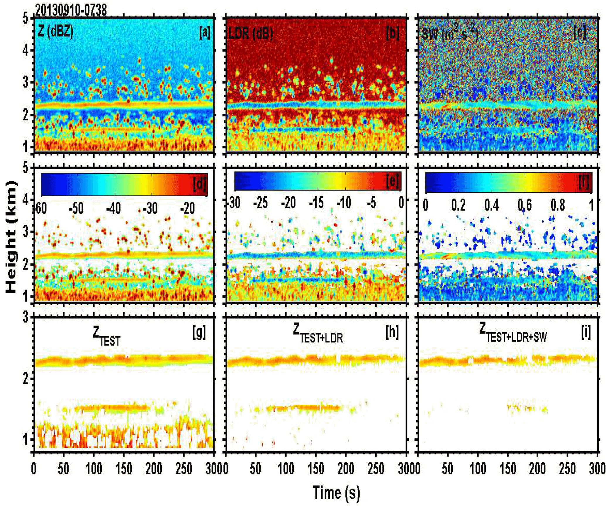
Figure 14 Same as Fig. 13 but for typical high-density biota noticeed at 07:38 UT on 10 September 2013.

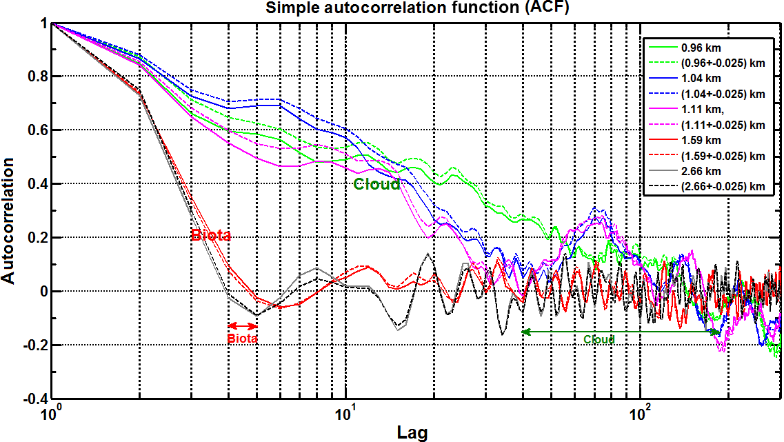
Figure 15 Simple ACF-inferred decorrelation periods associated with base (green line), middle (blue line), and top (magenta line) height levels of shallow cumulus cloud and biota height levels.

The merit of TEST algorithm lies mainly in its ability to recover shallow cumulus clouds present with biota. Figs. 13 and 14 are the typical examples to demonstrate the performance of TEST on screening out the shallow low-level clouds. These are the concluding figures, in which TEST (first column panels), LDR (second column panels) and SW (last column panels) measurements are all considered. The top and middle row panels are unfiltered and filtered, respectively, for noise using the S5 curve. In the noise-filtered data, both cloud and biota echoes at the lower level can be seen separately with middle panels of Figs. 13–14. The higher-level biota are more organized just above 2.5 km. Shallow ABL cloud regions show LDR values <−20 dB whereas insects show varied LDR values in the range of −25 to −5 dB. Thus, LDR alone is not sufficient to remove all insects (Fig. 13e). Smaller echo coherence periods associated with biota are further confirmed with smaller spectral width values (< 0.3 m² s⁻²; Fig. 13f). Higher spectral width values, on the order of ∼ 1 m² s⁻² of the cloud, indicate that the random motion of the smaller particles of cloud within the radar scattering volume is affected by the ABL turbulence. The discussed TEST algorithm (Fig. 13g) is able to screen out the cloud and filter out the biota significantly. Further, TEST fails to isolate relatively stronger biota returns existing within the cloud due to the lack of strong reflectivity gradient (both in short intervals of height and timescale), which fails to give the required high SD values to filter out biota. In order to ensure those echoes as biota and then to isolate those returns, the LDR values larger than −14 dB and SW values much smaller than 0.5 m² s⁻² have been chosen here. Isolated biota returns outside the cloud identified by TEST and the above critical thresholds with LDR and SW are found to be similar, except in a few places. It infers that the threshold value fails to filter out all biota returns due to either persistently low LDR or high SW values associated with those biota. However, it can be seen in Fig. 14 (similar to Fig. 13 but a typical case of high number density of biota on 10 September 2013 during 07:38–07:42 UT) that TEST alone is unable to remove biota (Fig. 14g), but by using LDR it becomes more promising (Fig. 14f). Furthermore, in the case of weakly turbulent cloud portions, they possess nearly comparable lower SW values as those of biota; under such conditions it is difficult to screen out clouds using SW alone (see Fig. 14i). Similarly, LDR alone cannot filter all biota and screen out weak clouds well. However, these two diverse and independent radar parameters, Doppler spectral width- and power-based polarimetric LDR measurements of KaSPR, will be an additional measure to identify cloud and non-hydrometeor radar echoes.

The above discussions suggest that the biota presence has been confirmed in more than one way, namely LDR and spectral width. LDR infers the liquid body presence in the atmosphere (e.g. cloud particle, bird or insect). Small values of spectral width suggest less velocity variance or small spread within radar sampling volume. The small velocity variance associated with isolated biota echo is obviously due to the sole presence of airborne biota that usually utilizes atmospheric dynamics (initially for flight up via convective updrafts and later via advection for horizontal flight at higher levels). Moreover, the limited velocity spread due to biota causes smaller spectral width than smaller, lightweight, volumetrically high-density cloud particles. Further, cloud particle are more vulnerable to small-scale local turbulence or entrainment processes that cause higher spread or dispersion of velocities to have high spectral width values associated with shallow cumulus cloud. Considering all these facts, it is interesting to note that the combined TEST, LDR and SW yields the best screened-out cloud results, where both cloud and biota co-exist within radar sampling height. Clouds show high spectral width values of ∼ 1 m² s⁻². Lower spectral width values pertinent to biota show that velocity variance of scatter within radar scattering volume is predominantly due to the presence of airborne biota (without much flight manoeuvre). This could be the reason for the smaller time coherence and degree of correlation of Z value with biota (e.g. 4–5 s) than clouds. Thus biota echo decorrelation times are small or quicker at the transmitted pulse scale. In order to confirm the precise decorrelation periods associated with the observed biota and cumulus clouds (Fig. 13a) that are assumed to be vertical radar transact across ABL, a simple autocorrelation function (ACF) has been used with the time series data of Z, corresponding to the biota at 1.59 and 2.66 km and cloud levels at the base, middle and top (single range gate (solid line) as well as averaged to its top and bottom range gate (dashed line)). The 0–300 s lag correlations of ACF for the cloud and biota are clearly seen with Fig. 15. Thus, from the ACF analysis it is clear that biota show quicker (∼ 4 s) decorrelation periods than cloud (∼ 40–170 s). Moreover, it is interesting to note that single height level (solid line) observations show relatively weaker correlation than average (dashed line); this is often seen with cloud echoes, which confirms that clouds have a high degree of phase coherence, mainly because clouds are widespread (in both time and space) in nature. High correlations seen with averaged cloud levels (dotted lines) suggest the highly in-phase (or coherent) nature of cloud echoes. Therefore, they constructively add. However, for incoherent nature of noise or biota, echoes add destructively. Thus, clouds show varied decorrelation periods above 30 s but biota mostly decorrelate in less than 10 s. Hence, the hypothesis proposed for TEST is proven here.

4 Summary and conclusions

Millimetre-band radars are very sensitive to the detection of small targets such as cloud droplets, insects and other biological particulates (biota) present in great numbers in the lower atmosphere. Polarization measurement is an efficient means to discriminate cloud echoes from non-hydrometeor scatterers that share very low reflectivity. Unfortunately not all radars are equipped with polarization measurements. This paper proposes, for these standard radars, a simple technique to separate meteorological and non-meteorological echoes. It uses only successive vertical reflectivity profiles acquired by a 35 GHz radar operated at vertical incidence with a 50 m pulse length and 1 s temporal sampling. Because of the high spatial and temporal resolution, most of the time only one (or no) biota target is present in the pulse resolution volume. In contrast, cloud echo is due to millions of droplets that occupy the pulse volume. As a consequence signal variability at a given range between two vertical profiles is much more important for biota scatterers than for cloud echoes. Signal variability is given here by the SD of the reflectivity over the course of four profiles, which corresponds to the typical duration of the biota echoes crossing the antenna beam. The threshold value that distinctly separates biota from cloud is obtained from statistical analysis of a large radar observation set. Indeed this value should be adjusted for a radar with different characteristics. This study responds to a real issue for anybody who wants to extract physical quantities from radar signal. The methodology used is validated with polarization measurements provided by the same radar.

It has been demonstrated that high-resolution vertically oriented zeroth moment (reflectivity) measurements of cloud radar are solely assured to segregate the hydrometeor and non-hydrometeor contributions with it. Theoretical NER curves are used to remove the system noise and importantly for recovering the weak cloud boundaries that are very closely hidden within the mean noise floor (curve S1) of the radar system. The simple statistical variance of continual radar echoes shows that the contrasting characteristics of signals like high dispersion (more than 2σ) are associated with the highly spurious and intermittent echoes of biota, and low dispersion (less than 1σ) is associated with coherent nature of echoes of cloud hydrometeors. For noise, dispersion is between 1.5 and 3.0σ. Furthermore, these characteristic features help demarcate the returns of cloud hydrometeor from those from biota and noise. Running mean and SD of offline reflectivity profiles for ∼ 4–5 s work well to filter out all non-hydrometeor returns. In this way, the time coherence of radar returns at every range sample was checked every 4 s, the offline window period to infer the decorrelation period associated with biota, which shows promise in identifying and filtering out the biota returns. The proposed TEST algorithm evaluates the observed cloud radar reflectivity profiles with combined theoretical radar sensitivity curves and statistical variance of radar echo and then tracks the cloud peak at either side to obtain the complete cloud height profile. In case of azimuth and elevation radar surveillance scans (PPI and RHI, for example), there is a regular change in the radar sampling area that prohibits an area-specific set of measurements required to perform the TEST method. But this method is advantageous and easily adaptable for better characterization of any high-resolution vertical profile measurements. The robustness of TEST is also proven through polarimetric and spectral width measurements and it is found that it works much better, particularly within the cloud region, at the cloud radar frequencies. TEST constrained using LDR was found to be promising under high-density biota conditions, whereas the superior performance of combined TEST constrained with both LDR and SW has been shown with highly turbulent shallow convective clouds. Such scrutinized reflectivity profiles have been further utilized to investigate the important CVS pertinent to the various phases of the ISM with the aim of improved prediction. Hence, the proposed TEST algorithm is able to extract the possible unbiased meteorological CVS information with the cloud profiling radar. This enables pragmatic, effective research investigations on seasonal and epochal tropical cloud characteristics.

Appendix A

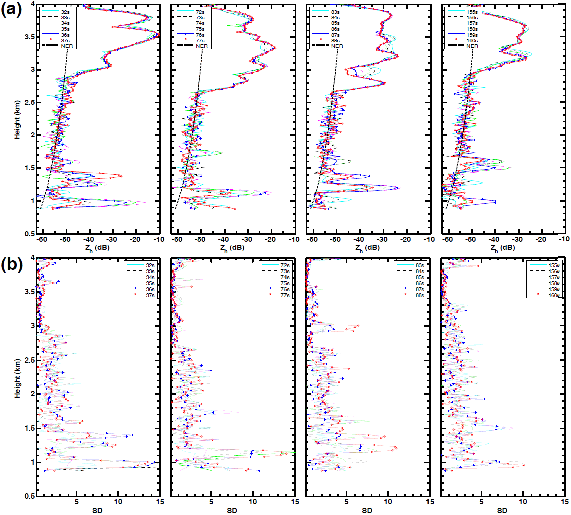
Figure A1 Instantaneous height profiles of Z during 12:00–12:05 UT on 29 May 2014 with centred number profile notice to be the strong biota return identified with HTI plot of Fig. 4b. (b) Corresponds to standard deviation (SD) from four-point running average.

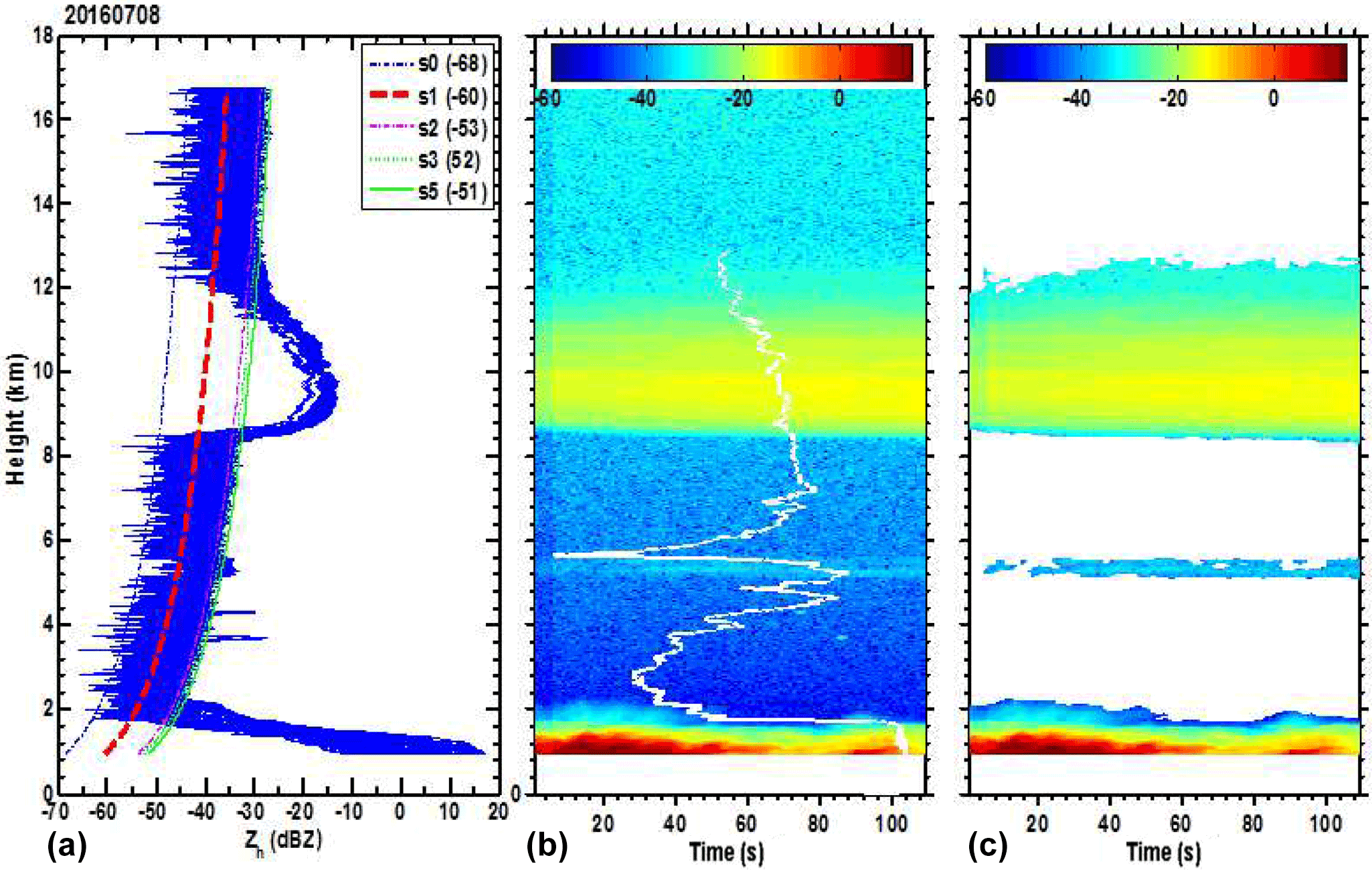
Figure A2 (a, b, c) Same as Fig. 1a–c but on 8 July 2016 during 05:31 UT for the duration of 108 s. S0–S5 are NER curves. Collocated GPS–RS relative humidity (%) profile is shown as a white solid line in (b).

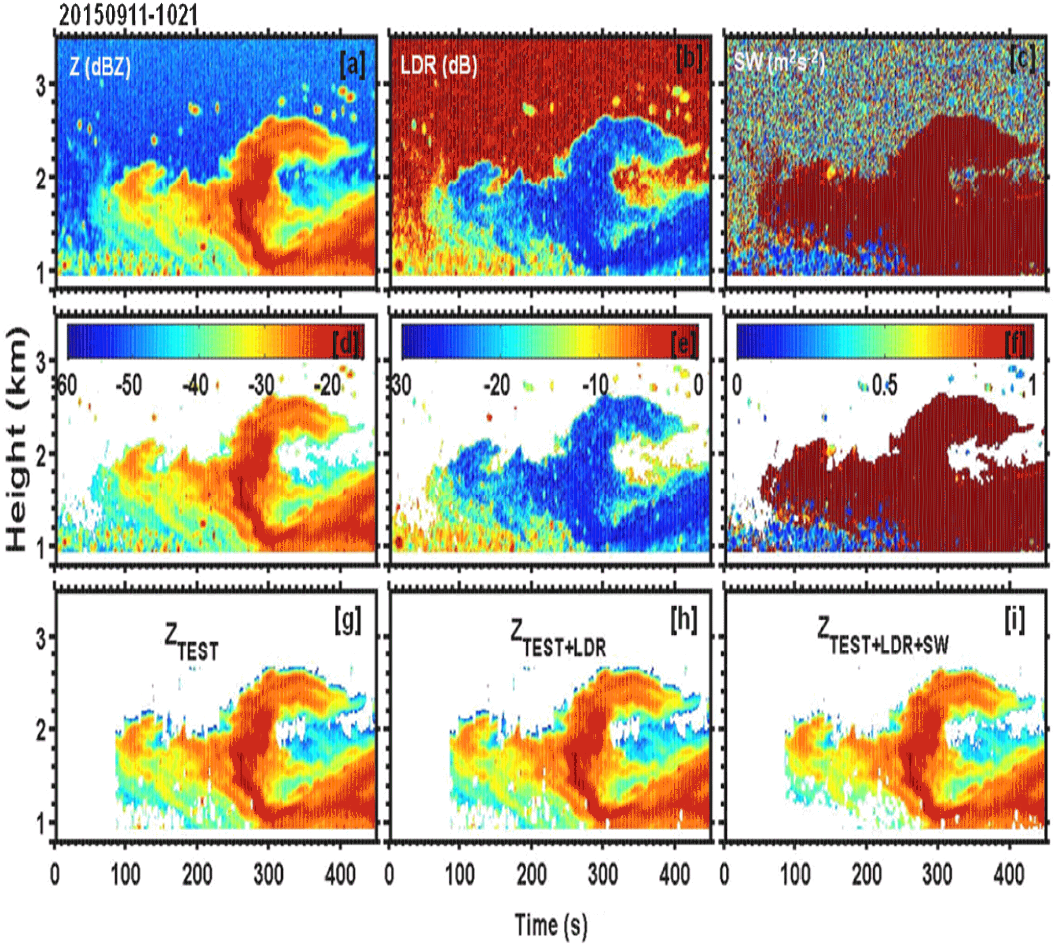
Figure A3 Same as Fig. 13 but during 10:21 UT on 11 September 2015 for the duration of 449 s.