Adaptive selection of diurnal minimum variation: a statistical strategy to obtain representative atmospheric CO₂ data and its application to European elevated mountain stations

Critical data selection is essential for determining representative baseline levels of atmospheric trace gases even at remote measurement sites. Different data selection techniques have been used around the world, which could potentially lead to reduced compatibility when comparing data from different stations. This paper presents a novel statistical data selection method named adaptive diurnal minimum variation selection (ADVS) based on CO₂ diurnal patterns typically occurring at elevated mountain stations. Its capability and applicability were studied on records of atmospheric CO₂ observations at six Global Atmosphere Watch stations in Europe, namely, Zugspitze-Schneefernerhaus (Germany), Sonnblick (Austria), Jungfraujoch (Switzerland), Izaña (Spain), Schauinsland (Germany), and Hohenpeissenberg (Germany). Three other frequently applied statistical data selection methods were included for comparison. Among the studied methods, our ADVS method resulted in a lower fraction of data selected as a baseline with lower maxima during winter and higher minima during summer in the selected data. The measured time series were analyzed for long-term trends and seasonality by a seasonal-trend decomposition technique. In contrast to unselected data, mean annual growth rates of all selected datasets were not significantly different among the sites, except for the data recorded at Schauinsland. However, clear differences were found in the annual amplitudes as well as the seasonal time structure. Based on a pairwise analysis of correlations between stations on the seasonal-trend decomposed components by statistical data selection, we conclude that the baseline identified by the ADVS method is a better representation of lower free tropospheric (LFT) conditions than baselines identified by the other methods.

1 Introduction

Continuous in situ measurements of greenhouse gases (GHGs) at remote locations have been established since 1958 (Keeling, 1960). Knowledge of background atmospheric GHG concentrations is key to understanding the global carbon cycle and its effect on climate, as well as the GHG responses to a changing climate. A critical issue when using data from remote stations remains the identification of time periods that are representative of larger spatial areas and their differentiation from periods influenced by local and regional pollution. If these two regimes are well disaggregated, the available datasets can represent more reliable information about long-term changes of undisturbed atmospheric GHG levels or be used to investigate local and regional GHG sources and sinks when specifically analyzing deviations from baseline conditions. In this study, the baseline conditions refer to a selected subset of data from the validated dataset, representing well-mixed air masses with minimized short-term external influences (Elliott, 1989; Calvert, 1990; Balzani Lööv et al., 2008; Chambers et al., 2016).

Measurement results depend on sampling methods, analytical instrumentation, and data processing. Validated data (labeled as VAL in this study to differentiate from the selected data) are usually obtained after signal correction, for example due to interferences from other GHGs such as water vapor, calibration accounting for sensitivity changes of the analyzer, and validation based on plausibility checks. Baseline data selection starts with validated data and identifies in subsequent steps a final subset of the validated dataset based on predefined criteria for specific qualities such as representativeness. These data will be referred to as “selected baseline data” or simply as “selected data” in the following.

Data selection methods can be categorized into meteorological, tracer, and statistical selection methods (Ruckstuhl et al., 2012; Fang et al., 2015). Meteorological data selection makes use of the meteorological information at the measurement sites, which provides valuable information about the surrounding environment as well as air mass transport (Carnuth and Trickl, 2000; Carnuth et al., 2002). Forrer et al. (2000), Zellweger et al. (2003), and Kaiser et al. (2007) intensively studied the relationship between measured trace gases (such as O₃, CO, and NO_x) and meteorological processes at Zugspitze, Jungfraujoch, Sonnblick, and Hohenpeissenberg. For CO₂, the most common parameters applied in the literature are wind speed and wind direction. They can provide information on critical variations at stations with sources and sinks in their vicinity, while these parameters are less suited at stations in largely pristine environments. For example, Lowe et al. (1979) performed a pre-selection on the CO₂ record at Baring Head (New Zealand) using periods with southerly winds only (clean marine air). Massen and Beck (2011) found that the CO₂ versus wind speed plot can be valuable for baseline CO₂ estimation without a local influence of continental measurements. Another widely used data filtering method is fixed time window selection, by selecting data in a certain time interval of the day based on local and mesoscale mechanisms of air mass transport. For selecting well-mixed air at elevated mountain sites, nighttime is usually chosen with a special focus on the exclusion of afternoon periods due to the influence of convective upward transport (Bacastow et al., 1985). Brooks et al. (2012), for example, limited their mountaintop CO₂ results in the Rocky Mountains (USA) by “time-of-day” from 0 a.m. till 4 a.m. local time (LT) to increase the likelihood of sampling the free tropospheric environment at the station. Apart from this, modeling techniques such as backward trajectories are very helpful for analyzing the origins and transport processes of air masses arriving at the station in detail (Cui et al., 2011). Uglietti et al. (2011) focused on the origins of atmospheric CO₂ at Jungfraujoch (Switzerland) by the FLEXible PARTicle dispersion model. Using tracers, data selection can be performed by investigating the correlations between the air components of interest. Many tracers have been tested and compared with CO₂. Threshold limits of 300 ppb for CO and 2000 ppb for CH₄ were defined by Sirignano et al. (2010) to perform a regional analysis of CO₂ data at Lutjewad (the Netherlands) and Mace Head (Ireland). Similar approaches with black carbon and CH₄ were performed by Fang et al. (2015) at Lin'an (China). Moreover, Chambers et al. (2016) applied a data selection technique to identify baseline air masses using atmospheric radon measurements at the stations Cape Grim (Australia), Mauna Loa (Hawaii, USA), and Jungfraujoch (Switzerland).

Unlike most of the methods mentioned above, which require additional data or advanced transport modeling, statistical data selection only relies on the time series of interest and typically investigates the variability of signal. It is usually assumed that the most representative CO₂ data are found during well-mixed conditions revealing small variations in time (Peterson et al., 1982) and in space (Sepúlveda et al., 2014). For continuous measurements, it is possible to investigate within-hour and hour-to-hour variability in the datasets. The within-hour variability is often expressed as the standard deviation of the measured data within 1 h. The hour-to-hour variability compares the differences between hourly averaged concentrations either during a certain time period, or from one hour to the next. Pales and Keeling (1965) marked ambient data as “variable” when the within-hour variability for the air sample was significantly larger than the within-hour variability for the reference gas. Consequently, they only considered CO₂ data to belong to background conditions when the concentrations were in “steady” conditions for 6 h or more. Similarly, Peterson et al. (1982) rejected sampled CO₂ data values for adjacent hours when the hour-to-hour variability exceeded 0.25 ppm. Thoning et al. (1989) combined these two strategies using an iterative approach by selecting data according to deviations of daily averages from a spline curve fit. Ruckstuhl et al. (2012) developed a method based on robust local regression, called “Robust Extraction of Baseline Signal”, to estimate the baseline curves generalized for atmospheric compounds, which is available in the R package IDPmisc (Locher and Ruckstuhl, 2012).

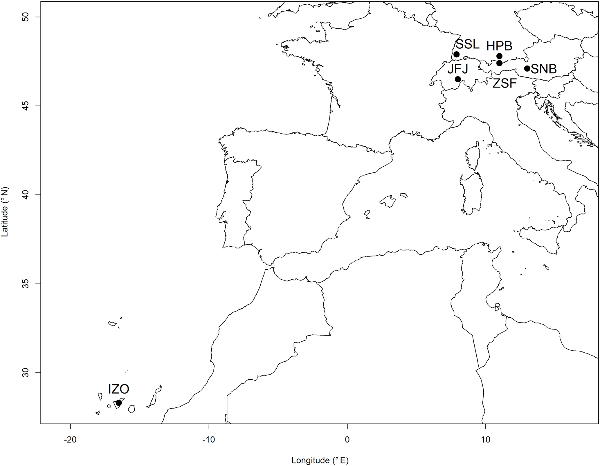
Figure 1 Locations of six European elevated mountain stations. Symbols from left to right stand for: IZO – Izaña, Spain; SSL – Schauinsland, Germany; JFJ – Jungfraujoch, Switzerland; HPB – Hohenpeissenberg, Germany; ZSF – Schneefernerhaus-Zugspitze, Germany; SNB – Sonnblick, Austria.

The present study focuses on the comparison of results from previous statistical data selection methods with the new adaptive diurnal minimum variation selection (ADVS) method proposed in this study. The ADVS is seen as a possible alternative to already known data selection methods as discussed above. The results obtained with ADVS for the atmospheric CO₂ records from six European mountain stations are compared with those derived from three other statistical data selection methods. To investigate the potential influences of trend and seasonality, further analyses focus on the decomposition of validated and selected datasets into trend and seasonal components. Finally, differences between ADVS and other data selection methods are assessed by correlation analysis.

2 Methods

2.1 CO₂ measurements at elevated European sites

CO₂ measurements from six European mountain stations (see Fig. 1) within the Global Atmosphere Watch (GAW) network were used. The data were taken from mountain stations due to their remote locations, being subjected to limited anthropogenic influence and this provided increased representativeness. Three high alpine measurement sites were included: Zugspitze-Schneefernerhaus (ZSF, DE, 47^∘25^′ N, 10^∘59^′ E, 2670 m a.s.l.), Jungfraujoch (JFJ, CH, 46^∘33^′ N, 7^∘59^′ E, 3580 m a.s.l.), and Sonnblick (SNB, AT, 47^∘03^′ N, 12^∘57^′ E, 3106 m a.s.l.). They are often above the planetary boundary layer (PBL) and thus exposed to free and presumably clean lower tropospheric air masses, but periodically influenced by regional emissions from lower altitudes. Additionally, to test data selection for a less remote environment, CO₂ measurements were investigated from Schauinsland (SSL, DE, 47^∘55^′ N, 7^∘55^′ E, 1205 m a.s.l.) at a much lower elevation, in the mid-range Black Forest. Data selection was also applied to three recently started CO₂ time series from different sampling heights above ground on a tall tower at the Hohenpeissenberg observatory (HPB, DE, 47^∘63^′ N, 11^∘01^′ E, 934 m a.s.l.), located in the northern foothills of the Alps. Henne et al. (2010) presented a method of categorizing site representativeness based on the influence and variability of population and deposition by the surface fluxes. JFJ and SNB were classified as “mostly remote,” while ZSF was considered as “weakly influenced, constant deposition,” and SSL and HPB were considered as “rural” (Henne et al., 2010). Finally, the station Izaña on Tenerife Island (IZO, ES, 28^∘19^′ N, 16^∘30^′ W, 2373 m a.s.l.) in the North Atlantic was chosen as a reference due to its location above the subtropical temperature inversion layer, which means that the station is rarely affected by any local or regional CO₂ sources and sinks (Gomez-Pelaez et al., 2013).

Table 1 Information of measured CO₂ datasets at six GAW mountain stations.

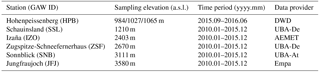
For this study, unless otherwise indicated, hourly data were used consistently for the purpose of evaluating the data selection method since the method should be easily applicable to data obtained from standard data centers such as the World Data Centre for Greenhouse Gases (WDCGG) where data are commonly stored with hourly resolution. The validated CO₂ hourly averages from all stations were downloaded from WDCGG (http://ds.data.jma.go.jp/gmd/wdcgg/). Data with higher time resolution required for some sensitivity analysis in this study were provided directly by the station investigators. All time stamps refer to the beginning of the averaging interval. Descriptions of the sampling elevation and time period of available data are given in Table 1. Further information on each station can be found in Schmidt et al. (2003) for SSL, Gilge et al. (2010) for HPB and SNB, Gomez-Pelaez et al. (2010) for IZO, Risius et al. (2015) for ZSF, and Schibig et al. (2015) for JFJ. Practical data selections and analyses in this study were performed using the R Statistical Environment (R Core Team, 2017).

2.2 ADVS

ADVS is a tool for automated and systematic analysis of diurnal CO₂ cycles at elevated mountain stations in order to select consecutive time sequences with minimum variation, which can be regarded as representing well-mixed air conditions. Even though such measurement sites are remotely located, the CO₂ levels are still influenced by local sources and sinks. For example, at ZSF, these can be characterized by episodic CO₂ enhancements due to anthropogenic emissions, detectable especially in winter during the day, whereas in summer the convective upwind transport results in episodes with depleted CO₂ concentrations due to photosynthetic uptake of CO₂ at lower altitudes. Although high altitude mountain stations do not have vegetation in their surroundings, mountain stations at lower altitudes that are still in the vegetation zone may be influenced by plant respiration, especially at night. As these effects of upward transport photosynthesis and respiration all vary diurnally, the basic strategy that we follow in this study is to identify the most stable time periods of the day, i.e., periods with minimum variation, which in turn can be used for selecting representative data. However, the duration of this time window during the day varies with the season and from day to day because of variations in the dynamics of transport to the site (e.g., Birmili et al., 2009; Herrmann et al., 2015). In summer, larger variabilities in the CO₂ signal are observed due to more prevalent convective boundary-layer air-mass injections influencing the diurnal pattern, resulting in shorter periods of stable conditions, whereas in winter, significantly longer stable periods occur. No upwind air masses with depleted CO₂ levels due to photosynthesis by vegetation are recorded in winter. To preserve as much representative data as possible, it is desirable to select the time window dynamically. ADVS is constructed to select a subset from the measured data, being best representative for baseline conditions with an adaptive selection time window specific for every day.

The algorithm is based on two basic assumptions. First, air masses measured at elevated stations represent well-mixed air, closest to baseline levels, within a certain time window of several hours during the day. For the elevated mountain stations discussed in this paper, this time interval is around midnight. Different diurnal patterns are apparent at each station, so the selection time window should be adjusted accordingly. Second, it is assumed that real baseline conditions are not subject to local influences and thus represent unperturbed lower free tropospheric air masses. This indicates that the variability of the measured CO₂ signal should be minimal within this selection time window. The methodological steps of ADVS are introduced in detail below in the two sections “starting selection” and “adaptive selection”.

2.2.1 Starting selection

For a given validated hourly dataset, ADVS starts data selection by finding a start time window for all days. The standardized selection procedure for the start time window results from site-specific parameters. This time interval is set as the most stable period from the diurnal variation. The step is referred to as starting selection. It begins by analyzing the mean diurnal cycle of the data input.

• Step 1: detrending is done by subtracting a 3-day average for each day, including the neighboring two days. It is the shortest possible time window to remove sudden changes in the time series related to the previous and posterior days while preserving the diurnal pattern.

• Step 2: the overall mean diurnal variation, ${\stackrel{\mathrm{‾}}{d}}_i$ (i=0 to 23 h), is calculated from the complete set of detrended data.

• Step 3: the standard deviations $s_{{\mathrm{\Delta }}_j}$ from the overall mean diurnal variation ${\stackrel{\mathrm{‾}}{d}}_i$ are calculated on a moving window Δ_j (j=6 h). To be able to place a full set of 24 moving time windows over the overall mean diurnal variation, time windows across midnight (e.g., 6 h from 11 p.m. to 4 a.m. LT) are also included, that is, its first j hours are appended to the end of the 24 h in the overall mean diurnal variation. The time window with the smallest standard deviation is selected as the start time window.

• Result: the start time window $\left[i_{\mathrm{start}},\mathrm{\dots },i_{\mathrm{end}}\right]$.

With the focus on elevated mountain stations, starting selection is purposely designed with the moving window Δ_j of 6 h, and the starting hour i_start to be between 6 p.m. and 5 a.m. LT for this study. For other stations with possibly different diurnal patterns, starting selection can be adjusted accordingly. For instance, at urban stations or stations completely within the continental PBL, the start time window can be chosen based on their best mixing conditions, which often occur in the afternoon with a shorter moving window, when the PBL reaches its maximum depth after “ingesting” free tropospheric air during its growth. Being aware that calculating the start time window from all data could differ from the start time windows calculated by season, the overall generated start time windows have been compared with seasonally generated start time windows for high altitude mountain stations (see Supplement Sect. S1.1). Because these differences were mostly small to moderate and this work aims at a methodical comparison under identical conditions, the start time windows are always derived from overall data.

2.2.2 Adaptive selection

The second component, adaptive selection, is designed to determine the most suitable time window for each day, based on the data variability. Through this method, the length of the start time window is expanded in both directions in time. Adaptive selection is performed on a daily basis, starting with the first day of the given dataset. The following steps only describe the forward adaptive selection. ADVS also runs the backward adaptive selection in an analogous manner but backwards in time.

• Step 1: the mean molar fraction ${\stackrel{\mathrm{‾}}{x}}_i$, standard deviation s_i, and the proportion of missing values π_missing are calculated from data in the start time window $\left[i_{\mathrm{start}},\mathrm{\dots },i_{\mathrm{end}}\right]$.

• Step 2: if s_i≤0.3 ppm (CO₂) and π_missing≤0.5, ADVS continues to advance in time, examine whether the next data point x_f can be included in the selection time window W with $f=i_{\mathrm{end}}+\mathrm{1}$. Otherwise, it is considered that the start time window does not fulfill the assumptions. In this case, no baseline data is selected for the present day and the algorithm proceeds to the next day.

• Step 3: the absolute difference between x_f and ${\stackrel{\mathrm{‾}}{x}}_i$ is calculated, and the following threshold criterion is applied: $\left|x_f-{\stackrel{\mathrm{‾}}{x}}_i\right|\le \mathit{\kappa }\cdot s_i$, where κ is the threshold parameter. If this criterion holds, x_f is included in W and ADVS continues. Otherwise, ADVS stops for this day with only the start time window, and proceeds to the next day.

• Step 4: mean ${\stackrel{\mathrm{‾}}{x}}_W$ and standard deviation s_W for the new selection time window W are calculated. If s_W≤0.3 ppm (CO₂), ADVS continues with the next data point x_f with $f=f+\mathrm{1}$. Otherwise, ADVS stops for this day with the previous selection time window and proceeds to the next day.

• Step 5: the new absolute difference between x_f and ${\stackrel{\mathrm{‾}}{x}}_W$ is calculated, as well as the new threshold criteria. If condition $\left|x_f-{\stackrel{\mathrm{‾}}{x}}_W\right|\le \mathit{\kappa }\cdot s_W$ holds, x_f is included in W and ADVS goes back to Step 4. Otherwise, ADVS stops for this day and proceeds to the next day.

  When data selection for all days is finished, ADVS continues with backward adaptive selection. Afterwards, it proceeds to the result.

• Result: this is the final selection time window, which is a combination of W_forward and W_backward for the day in question.

The following limitations of the forward and backward expansions of the time window should be considered. ADVS always runs for no longer than 24 h including the start time window, i.e., $f\le \mathrm{24}\cdot$ tr, where tr is the time resolution in data points per hour of the input data. This sometimes results in an overlap of “selected” and “unselected” data for two consecutive days. We always label the data as “selected” once it has been selected by ADVS. The threshold parameter κ is the controlling factor for the length of the selection time window. As κ increases, the length of the selection time window increases. A value of 2 was chosen heuristically for this study as a compromise between selecting as many data points as possible and achieving the least data variability. Similar values of sensitivity-controlling parameters in other data selection methods can be found (Thoning et al., 1989; Sirignano et al., 2010; Uglietti et al., 2011; Satar et al., 2016). In Step 2, values of 0.3 ppm and 0.5 indicate the threshold values for s_i and π_missing. We denote them as s_i,threshold and π_{missing,threshold}. Less remote stations at lower altitudes may require a larger value than 0.3 ppm because of different mixing conditions. When performing ADVS data selection at lower sites such as HPB and SSL, we recommend a higher s_i,threshold, such as 1.0 ppm. However, throughout this study we used the described parameter setting (0.3 ppm) for a methodical inter-comparison of selection methods at all stations. Potential influences of these parameter sizes (s_i,threshold and tr) are discussed in Supplement Sect. S1.2 and S1.3.

2.3 Other statistical data selection methods for comparison

We compared ADVS with three statistical data selection methods. The first method named SI is based on “steady intervals” (Lowe et al., 1979; Stephens et al., 2013). Steady intervals, which are considered as baseline conditions, are defined by a standard deviation being lower than or equal to 0.3 ppm for six or more consecutive hours. Although this method has some similarity with ADVS, it treats all hours of the day equally without giving preference to hours where the variability is, on average, the smallest.

Second, we adopted a method applied by NOAA ESRL, which originated from Thoning et al. (1989). This selection routine has been applied specifically for measurements of background CO₂ levels at Mauna Loa. This method (referred to as THO) was applied as described on the website: http://www.esrl.noaa.gov/gmd/ccgg/about/co2_measurements.html. The first step of THO examines the within-hour variability by selecting hours with hourly standard deviation less than 0.3 ppm. For the hourly data used in this study, the within-hour variability is not applicable so that the first step is skipped. Second, it computes hourly averages and checks the hour-to-hour variability by retaining any two consecutive hourly values where the hour-to-hour difference is less than 0.25 ppm. The last step is based on the diurnal pattern (similar to ADVS), by excluding data from 11 a.m. to 7 p.m. LT due to transported air influenced by photosynthesis.

The last method compared is a moving average technique (MA). A moving time window of 30 days and a threshold criterion of two standard deviations from the moving averages were applied to discard outliers. Afterwards, new moving averages and new threshold criteria were calculated for data exclusion. This step is repeated until no more outliers were found. A more detailed description can be found in Uglietti et al. (2011) and Satar et al. (2016).

2.4 Seasonal-trend decomposition STL

To analyze the results from different data selection methods and compare them with the original validated datasets, we applied the seasonal-trend decomposition technique based on locally weighted regression smoothing (Loess), named STL (Cleveland, 1979; Cleveland et al., 1990). STL has been widely applied to measurements of atmospheric CO₂ and other trace gases (Cleveland et al., 1983; Carslaw, 2005; Brailsford et al., 2012; Hernández-Paniagua et al., 2015; Pickers and Manning, 2015). It decomposes a time series of interest into a trend component T, a seasonal component S, and a remainder component R, which allows detailed separate analyses of trend and seasonality. Two recursive procedures are included in the STL technique: an inner loop where seasonal and trend smoothing based on Loess are performed and updated in each pass, and an outer loop that computes the robustness weights to reduce the influences of extreme values for the next run of the inner loop (Cleveland et al., 1990).

For this study, we used the implemented function stl in R (R Core Team, 2017). Owing to functional limitation of stl, full time coverage of monthly data is needed in order to reduce the risk of large time gaps or unequal spacing (Pickers and Manning, 2015). All data were first aggregated to monthly averages. Then, missing data were substituted by linear interpolation, using R function na.approx (Zeileis and Grothendieck, 2005). For the application of STL, two parameters need to be specified, which are the seasonal smoothing parameter n_(s) (s-window in function stl) and the trend smoothing parameter n_(t) (t-window in function stl). As n_(s) and n_(t) increase, the seasonal and trend components get smoother (Cleveland et al., 1990). For optimal compatibility in this study, the same parameters were chosen for all stations as n_(s)=7 and n_(t)=23, based on the recommendation of Cleveland et al. (1990). Another parameter combination of n_(s)=5 and n_(t)=25 was also tested according to Pickers and Manning (2015), but with no significant differences in results.

3 Results and discussion

3.1 Start time window

ADVS was applied to the validated hourly averages from all six stations with the parameter settings as described above. The detrended mean diurnal cycles were obtained together with the start time window for each station by starting selection (see Fig. 2, for conventional mean diurnal plots see Supplement Sect. S2). The observed differences in the start time windows, as well as in the widths of the confidence intervals (gray shades), reflect the characteristics of differently situated measurement sites and different sampling levels. The first subplot column (HPB50, HPB93, and HPB131), representing the three sampling heights at HPB, shows similar detrended diurnal patterns with similar start time windows. The slightly different start time window at HPB131 potentially indicates different dynamics of the atmospheric transport at higher elevation. The decreasing amplitude with increasing sampling height indicates that the higher the sampling inlet is above the ground, the less it is affected by the local surface fluxes. The three start time windows suggest that the most stable period at HPB occurs during the last few hours of a day, including midnight. However, in contrast to all other stations covering at least a full year, HPB data are only from September of 2015 to June of 2016. The results may not be fully comparable, but instead it shows that the data selection method is also applicable to data with time periods shorter than one year.

Figure 2 Detrended mean diurnal cycles of validated CO₂ datasets (black) with 95 % confidence intervals (gray) from six GAW stations (hours in LT). Measurements at HPB are differentiated by the sampling heights (e.g., HPB50 for 50 m a.g.l.). The covered time periods (top text), resulting start time windows (middle text, also in light blue shades), and mean diurnal amplitudes (bottom text) are shown in each subplot.

Regarding the second subplot column (SSL, SNB, and IZO), the start time windows can be found from midnight on or later in the morning. The start time window for SSL encompasses its diurnal maximum, indicating that data variability is considerably smaller in the early morning than in the afternoon because of its vicinity to the Black Forest region, which has strong influence due to local photosynthetic activity (Schmidt et al., 2003). A similar diurnal pattern can be found at SNB. The influence of CO₂ sources is not as prominent as the effect of distant CO₂ sinks, since it is situated at the isolated summit peak of Hoher Sonnblick surrounded only by mountains and glaciers, with a negligibly small number of tourists, thus anthropogenic activities are minimal. IZO is a special case, since it is located on a remote mountain plateau on the Island of Tenerife above the strong subtropical temperature inversion layer. Even though the start time window is limited to 6 h, IZO presents an ideal mean diurnal cycle for data selection from a potentially much longer time window.

In the right column of the figure, both ZSF and JFJ find their start time windows around midnight (including hours after midnight). ZSF shows higher diurnal CO₂ amplitude than JFJ, but the two sites show similar diurnal patterns. For the choice of the start time window from the mean diurnal variation, relatively close or even local anthropogenic sources may influence the CO₂ at these two stations, possibly due to touristic influences.

3.2 Percentage of selected data

Starting from the initial start time windows, ADVS selected the baseline data for all stations (see Fig. 3). In addition, we calculated the percentages of the complete datasets selected by ADVS as baseline data, which are listed in the first column of Table 2. The higher the percentage the more well-mixed air is measured at the station, which is assumed to be a representation of lower free tropospheric conditions. This holds especially for IZO, where a larger percentage of 36.2 % was selected as baseline data. The sites with intermediate percentages are JFJ (22.1 %), SNB (19.3 %), and ZSF (14.8 %). For the three sampling heights at HPB, only 3.2 % (50 m), 4.8 % (93 m), and 6.2 % (131 m) of the data were selected by ADVS. Finally, a similarly low percentage was found for SSL (4.0 %), probably due to its higher data variability.

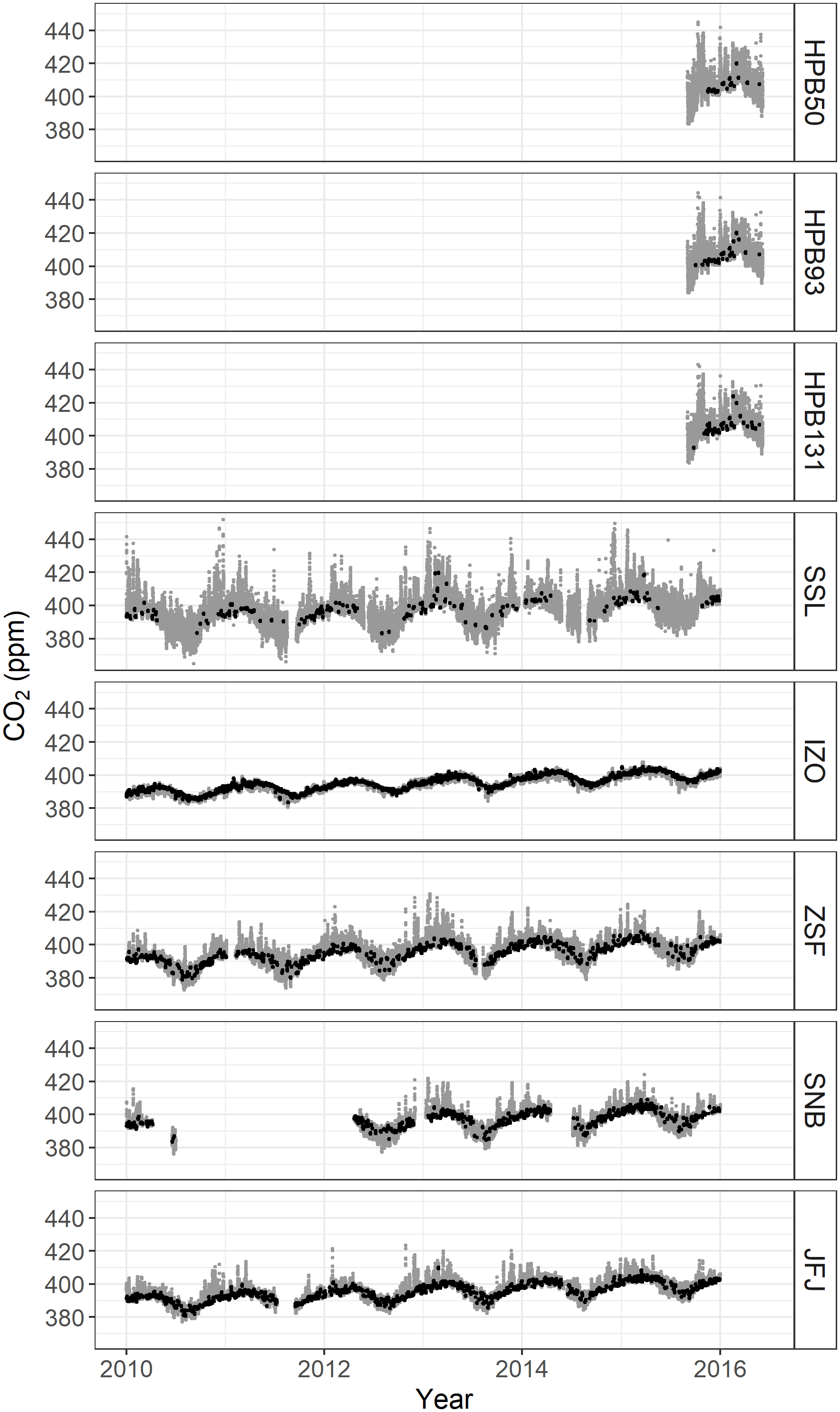
Figure 3 Time series plots of validated CO₂ datasets (gray), and selected datasets by ADVS (black) at six GAW stations.

Table 2 clearly indicates that the percentage of baseline data increases with altitude for all methods, suggesting measurements at higher altitudes can capture progressively well-mixed and hence representative air. Based on this finding, a linear least squares regression was applied between the absolute altitudes and the percentages of selected data for continental stations. IZO is on a remote island and therefore not comparable. This approach reveals a significant positive linear trend (see coefficient in Table 2). The related figure of linear regression can be found in Supplement Sect. S3.1.

To examine the characteristic growth of the percentages of selected data by ADVS during the selection process, we additionally calculated percentages after completing both the starting selection and adaptive selection steps mentioned in Sect. 2.2 (see Supplement Sect. S3.2). All results of percentages show an order of stations similar to that above, and the percentages increase steadily step by step for all stations. The percentages of selected data by ADVS were then compared with those of the mentioned statistical data selection methods SI, THO, and MA (see Table 2, with the corresponding figure shown in Supplement Sect. S3.3).

Table 2 Percentage of selected data in all data by different data selection methods. The bottom shows the linear regression coefficients of station (HPB is represented by HPB50; IZO is excluded) altitudes and the percentages of selected data at the significance level of 0.05 (${}^{\ast \ast \ast }$).

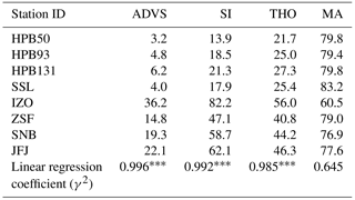
Since the percentages of selected data indicate not only the amount of data declared as representative but also show the characteristics of the selection methods, this criterion is used for further assessment. All other methods except for MA result in higher percentages for higher altitude stations (IZO, ZSF, SNB, and JFJ) than for those of lower altitudes (HPB and SSL). ADVS always performs the strictest filtering in all cases. Based on the stepwise study (see Supplement Sect. S3.2), these low percentages are primarily due to the restrictive definition of the start time window requiring data with a standard deviation of less than 0.3 ppm. With adaptive selection, the percentages of selected data increase but remain lower than those of the other methods. SI and THO, in comparison, show differences between stations at high and low elevations. Compared with SI, THO is higher at stations at lower elevations, but lower at high ones. A major limitation of SI seems to be the requirement for consecutive hours, in our case of 6 h with 0.3 ppm standard deviation threshold, which might be too restrictive for stations at lower elevations. However, this criterion results in a fairly large percentage for stations at high elevations. At ZSF, SNB, and JFJ, it results in the second largest, and even the largest in the case of IZO.

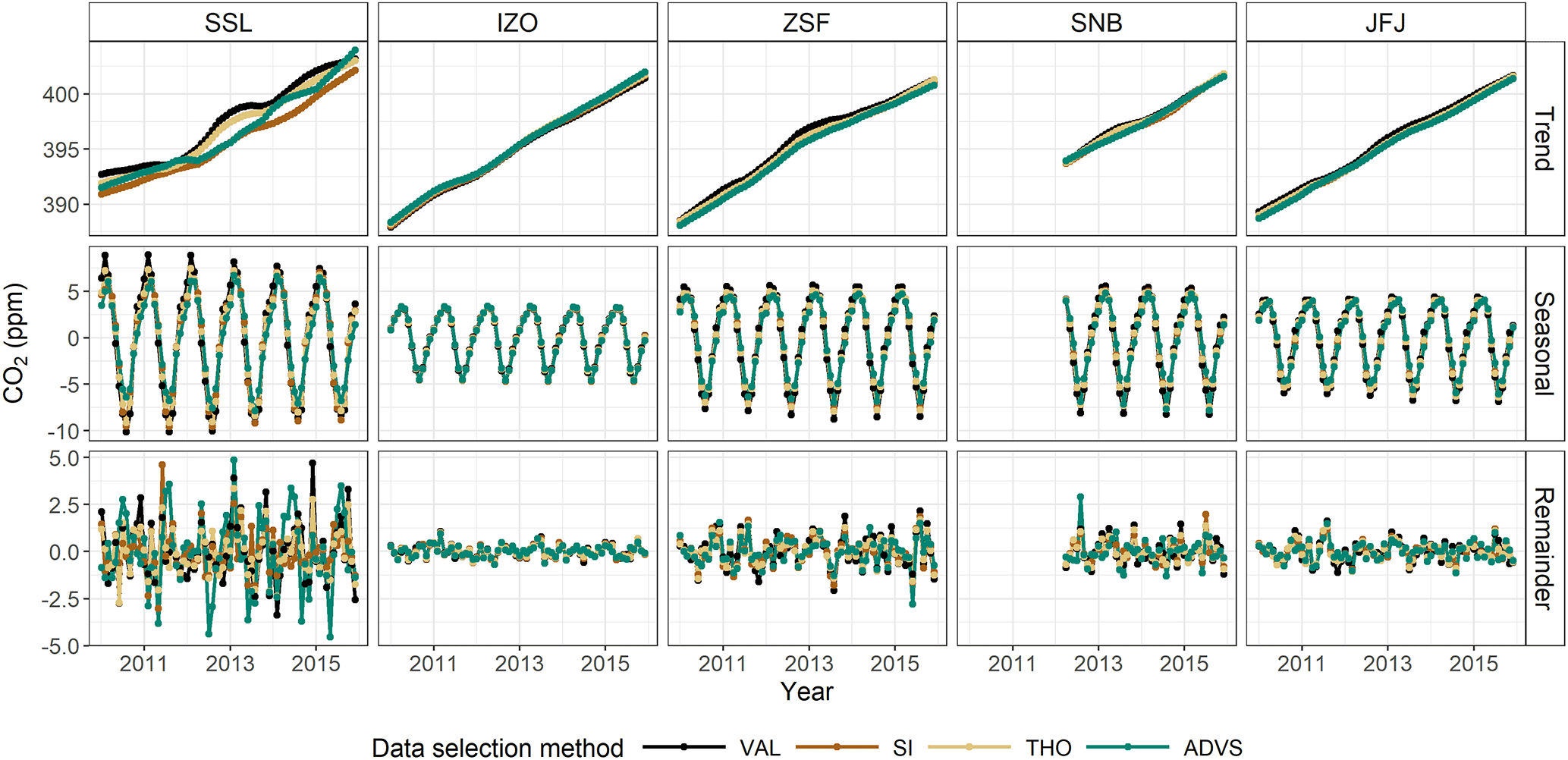
Figure 4 STL decomposition results from VAL (black), SI-selected (brown), THO-selected (yellow), and ADVS-selected (green) datasets at five GAW stations.

The highest percentages of selected data (approximately 80 %) were obtained with MA at most stations except for IZO. However, IZO obtains the largest percentages from all other selection methods. This is probably caused by the very low variability of CO₂ at IZO, resulting in overly strict moving-average thresholds for the MA method. Thus, we conclude that MA does not work properly in the case of very well-mixed air (IZO). At all other stations, it is possible that MA declares too much data as representative. Therefore, MA was excluded from further analyses.

3.3 STL components

STL was applied to the validated datasets before and after baseline selection with SI, THO, and ADVS, except for HPB due to its limited length of time (less than one year). Depending on data availability, STL was performed on CO₂ data from 2012 to 2015 at SNB, while data inputs at SSL, IZO, ZSF, and JFJ cover the whole period from 2010 to 2015. Figure 4 gives an overview of the decomposition by STL. The following sections discuss the resulting components obtained by STL, namely the trend component, the seasonal component, and the remainder component.

3.3.1 Trend component

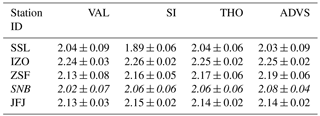
From the trend components, the mean annual growth rates were estimated by linear regression (see Table 3). Based on the 95 % confidence intervals for the slope, positive trends i.e., increasing CO₂ concentrations are observed. Owing to the overlap of the confidence intervals, differences in the mean annual growth rates among VAL and selected datasets at the same station are all in good agreement. This indicates that the trend component is not significantly influenced by the statistical data selection method, which agrees well with the finding of Parrish et al. (2012) from a study of baseline ozone concentrations that there were no significant differences of the long-term changes between the baseline and unfiltered datasets. Moreover, the following fact is observed for all sites except for SSL. Compared to unselected data (VAL), the mean annual growth rates based on selected datasets are systematically higher approaching the growth rates at IZO. IZO can be considered as better representing the lower free tropospheric conditions and agrees well with the mean annual global CO₂ growth rates (2.31 ppm) during the same time period (2010–2015) based on data from https://www.esrl.noaa.gov/gmd/ccgg/trends/global.html. The exception at SSL is probably caused by stronger local influences as a result of its lower elevation. In addition, the confidence intervals of the mean annual growth rates are always smaller after data selection, which improves the precision of trends.

Table 3 Mean annual growth rates (ppm yr ⁻¹) with 95 % confidence intervals from linear regression, applied on the trend components by STL over 2010 to 2015, except for SNB. Data at SNB were decomposed over 2012 to 2015 due to missing data from 2010 to 2011 and thus shown in italic font.

3.3.2 Seasonal component

The resulting seasonal components show systematic differences between VAL and selected datasets. The mean monthly variations were calculated on a monthly scale over the entire period from the analyzed data. Figure 5a and b present the results at stations ZSF and IZO. At most stations (except for IZO), the seasonal amplitudes have been substantially reduced compared to VAL (see also Fig. 4). At ZSF, the averaged peak-to-peak seasonal amplitude, defined as mean seasonal maximum minus seasonal minimum, drops the most by 18.9 % from VAL with the ADVS selected dataset. An explanation of this reduction is CO₂ signal exclusion from local sources and sinks by data selection. When taking a closer look at the monthly averages, lower CO₂ values are found in the selected datasets in the winter months from October to April, indicating that the CO₂ concentrations estimated by VAL are above the background levels because of more dominant anthropogenic activities and no active vegetation. Higher values in the summer months from May to September explain underestimation of VAL due to intensified upward transport of photosynthetic signatures resulting from vegetation. Similar patterns can be found at stations SSL, SNB, and JFJ (see Supplement Sect. S4). IZO always shows the smallest seasonal amplitude and there is almost no difference between VAL and selected datasets. Based on this consideration, it is very likely that the lower free troposphere will react with a delay to CO₂ concentration changes of effective sources and sinks on the ground, acting like an atmospheric memory.

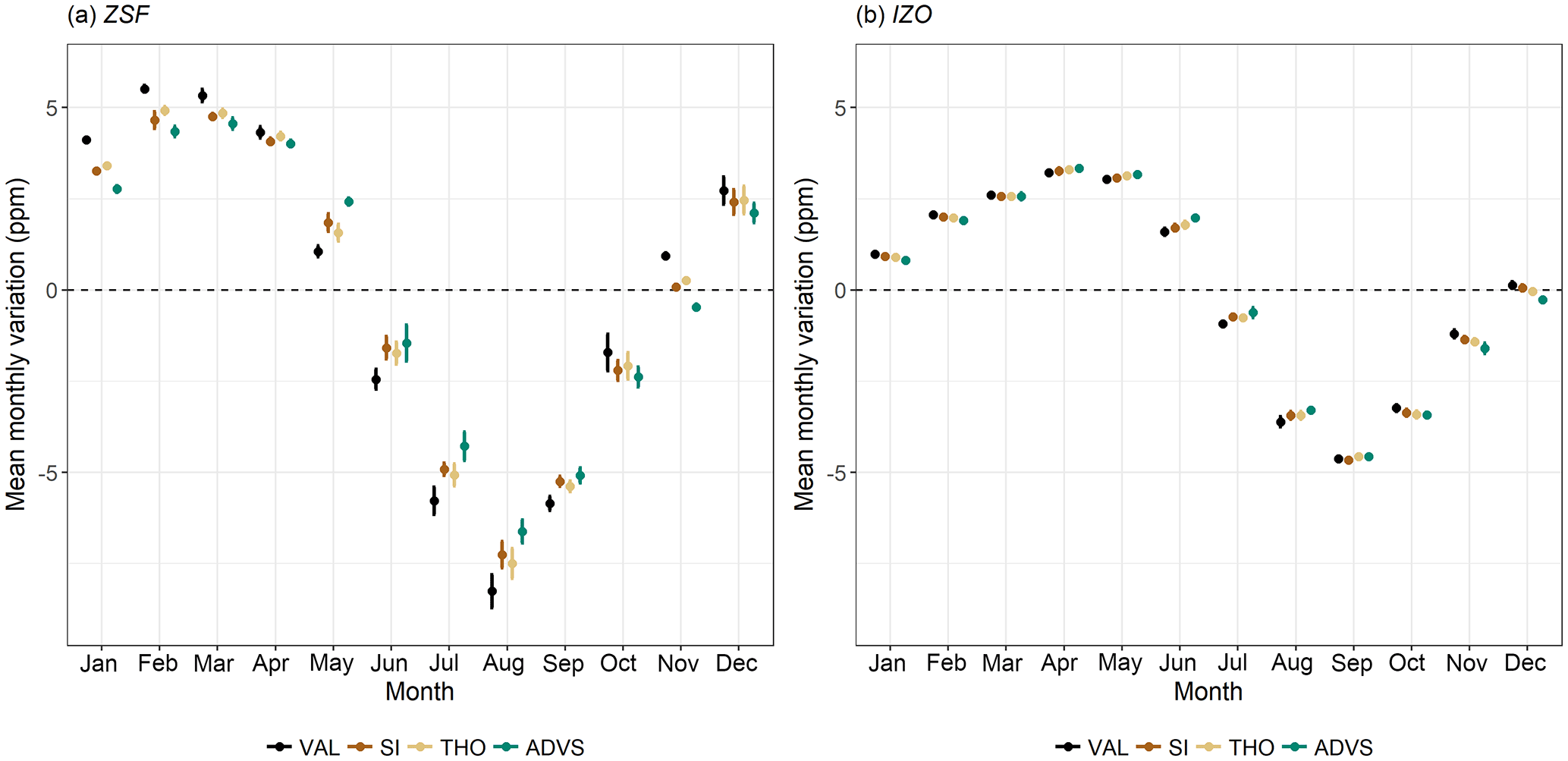
Figure 5 Mean monthly variation of the seasonal component decomposed by STL at (a) ZSF and (b) IZO over the whole period. For a better visualization of the results of selection methods, dots have been separated horizontally and equidistantly. The 95 % confidence intervals are shown as error bars.

A time delay of one month in the mean seasonal maximum is shown in Fig. 5a at ZSF with selected datasets by SI and ADVS (March), compared with the maximum from the validated data (February). A similar time shift can also be found by other selection methods at stations SSL (one-month delay from February to March by SI and ADVS) and JFJ (two-month delay from February to April by SI, THO, and ADVS). As for station IZO (April) in Fig. 5b and station SNB (March), the seasonal maxima stay the same. The magnitude of these delays may be related to mixing in the lower free troposphere. Rapid changes are usually observed close to sources and sinks, e.g., from anthropogenic and biogenic activities. Thus, the higher the station is above the boundary layer, the later the maxima during the winter can be observed because of the late response due to inhibited mixing. However, this delay does not occur for the minima during the summer because of the very effective upward transport and more favorable mixing conditions at that time of year. Consequently, no change in the seasonal minima is observed at all measurement sites, which is taken as an indicator of enhanced thickness of the mixing layer as good mixing conditions. Taking ZSF as an example, Birmili et al. (2009) observed low concentrations of particle numbers in winter and found it representative for the free tropospheric air by analyzing the annual and diurnal cycles. From spring onwards, the PBL rises with increasing temperatures. The intense vertical atmospheric exchange during summer months results in a daily air mass transport from the boundary layer to reach ZSF due to thermal convection (Reiter et al., 1986; Birmili et al., 2009). Thus there are optimal transport and mixing conditions. Therefore after data selection, the timing of seasonal peaks corresponds better among the stations.

Figure 6 Pearson's correlation matrices of combinations of trend and seasonal components (T+S, a), and only remainder components (R, b) at stations SSL, IZO, ZSF, SNB, and JFJ by different selection methods. Correlations with no significant coefficients at the 0.05 significance level were left blank.

3.3.3 Remainder component

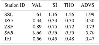
The remainder component resembles random noise from local influences in its structure, being different from site to site and statistically uncorrelated with the general signal of CO₂ concentrations in the lower free troposphere (Thoning et al., 1989). The standard deviation of the remainder component is taken here as a measure for external influences (see Fig. 4). Table 4 shows the calculated standard deviations from the remainder components at each station. Comparable results are derived from all selected datasets. SSL, as the lowest altitude station, exhibits the largest variation. IZO with the smallest standard deviations in the remainder component proves to be the station least influenced by its surrounding environment. The three alpine measuring stations (ZSF, SNB, and JFJ) exhibit intermediate variability. From this perspective, STL performs well in showing the site characteristics. Consequently, the noise of the remainder components, given in Table 4, decreases with increasing altitude of the continental mountain stations, which is in inverse relation to the percentages of selected data (Table 2). IZO was excluded in both regressions against altitude because of its maritime character.

Table 4 Standard deviations of the remainder components by STL over 2010 to 2015, except for SNB. Data at SNB were decomposed over 2012 to 2015 due to missing data from 2010 to 2011 and thus shown in italic font.

3.4 Correlation analysis

As mentioned above, data selection is defined here as an approach of extracting a group of data to be the best representative for the lower free troposphere. Consequently, the selected CO₂ datasets should have properties that are well correlated between the sites. For evaluating this hypothesis, we took the combination of the trend and seasonal components from STL and examined the correlations between each pair of stations in a Pearson correlation matrix (see Fig. 6a). The trend and seasonal components of all VAL and selected datasets were first compiled, and then Pearson's correlation coefficients were calculated assuming normal distribution of data examined by the Anderson–Darling test (P < 0.05). The correlation matrices are shown for each data selection method individually, in order to enable a comparison between ADVS and other methods. Data used for correlation were chosen only when available at all stations (2012–2015). In general, most pairs show higher correlation coefficients with selected data irrespective of the selection method, especially between the three Alpine stations (ZSF, SNB, and JFJ). This evaluation shows a similar result to the method presented by Sepúlveda et al. (2014) for identifying baseline conditions based on the correlation between distant measuring stations. Pairs including IZO after data selection by ADVS show a notable increase in the correlation coefficients, meaning better coherence between the reference station IZO and the others.

Conversely, when selecting representative data more effectively, the results should contain less local and regional influences. Therefore, we compared the remainder components derived from STL pairwise to check whether the Pearson correlation coefficients decreased after data selection (see Fig. 6b). The number of insignificant correlations between the station pairings is the greatest for ADVS. For the only two coefficients significant at the 0.05 significance level (ZSF-SNB and ZSF-JFJ), they drop largely from 0.75 to 0.48, and from 0.75 to 0.40, respectively, which cannot be observed by the other selection methods. This means that by ADVS the combination of trend and seasonal components correlate best and the remaining unselected data have the lowest correlation among the methods. If these two criteria are used to separate the representative part of the data from the unrepresentative part, the ADVS method produces the best results.

4 Conclusions and outlook

We presented the novel statistical ADVS method for selecting representative baseline data for CO₂ measurements at elevated GAW mountain stations. For assessment of the data selection procedure, we applied the method to six CO₂ datasets measured at GAW mountain stations in the European Alps. The ADVS resulted in an increasing number of percentages of selected data representing the background conditions with growing altitude of continental measurement sites, which is reasonable due to the underlying atmospheric dynamics. For comparison, three well-known statistical data selection methods were applied to the same datasets and most methods yielded similar increasing percentages with growing altitude. Among all the methods, ADVS is the most restrictive in terms of the number of selected data in the overall datasets.

In addition, we applied the time series decomposition method STL to all datasets before and after data selection. All statistical data selection methods resulted in the same annual trend within the 95 % confidence interval of the datasets before selection, while the seasonal signal varied substantially with smaller seasonal amplitudes and delayed occurrences of seasonal maxima. We also presented an additional assessment of ADVS compared with the other statistical data selection methods based on correlation analysis. For the combination of trend and seasonal components by STL, higher correlation coefficients between stations were found with ADVS data selection than SI and THO. Inversely, ADVS resulted in lower correlation coefficients in the remainder components than the other methods. Both indicate a better performance of selecting baseline data by ADVS.

The presented method is useful for data selection of atmospheric CO₂ data representative of the lower free troposphere. It requires only data from a single measurement site, is easily adjustable to the local conditions, and runs automatically. The method can also be applied to historical datasets. The results provide evidence that the proposed ADVS method confers the possibility of selecting data that are representative of CO₂ concentrations of a larger area of the lower free troposphere. This is an elementary prerequisite for application of the method to a larger number of different stations and an essential step towards generalization. It directly supports the objective of GAW to extrapolate from a set of point measurements from single stations to a larger representative area or region in the lower free troposphere (WMO, 2017). In future, there is a need to test whether such results could be used for additional applications, such as ground calibration of satellite measurements. Finally, it would be very interesting to test as a next step whether this presented method is applicable to stations in other regions and on other continents. Moreover, the issue of whether and how to include coastal stations in a systematic and practically generalizable approach for selecting representative data at GAW stations will be a particular concern.