Vertical wind velocity measurements using a five-hole probe with remotely piloted aircraft to study aerosol–cloud interactions

The importance of vertical wind velocities (in particular positive vertical wind velocities or updrafts) in atmospheric science has motivated the need to deploy multi-hole probes developed for manned aircraft in small remotely piloted aircraft (RPA). In atmospheric research, lightweight RPAs (< 2.5 kg) are now able to accurately measure atmospheric wind vectors, even in a cloud, which provides essential observing tools for understanding aerosol–cloud interactions. The European project BACCHUS (impact of Biogenic versus Anthropogenic emissions on Clouds and Climate: towards a Holistic UnderStanding) focuses on these specific interactions. In particular, vertical wind velocity at cloud base is a key parameter for studying aerosol–cloud interactions. To measure the three components of wind, a RPA is equipped with a five-hole probe, pressure sensors, and an inertial navigation system (INS). The five-hole probe is calibrated on a multi-axis platform, and the probe–INS system is validated in a wind tunnel. Once mounted on a RPA, power spectral density (PSD) functions and turbulent kinetic energy (TKE) derived from the five-hole probe are compared with sonic anemometers on a meteorological mast. During a BACCHUS field campaign at Mace Head Atmospheric Research Station (Ireland), a fleet of RPAs was deployed to profile the atmosphere and complement ground-based and satellite observations of physical and chemical properties of aerosols, clouds, and meteorological state parameters. The five-hole probe was flown on straight-and-level legs to measure vertical wind velocities within clouds. The vertical velocity measurements from the RPA are validated with vertical velocities derived from a ground-based cloud radar by showing that both measurements yield model-simulated cloud droplet number concentrations within 10 %. The updraft velocity distributions illustrate distinct relationships between vertical cloud fields in different meteorological conditions.

1 Introduction

Vertical wind is a key parameter for understanding aerosol–cloud interactions (ACIs). In tracing the evolution of aircraft-based wind measurements in the atmosphere, three axes of development have been pursued since the 1960s: improvements in airborne platforms, inertial navigation systems (INSs) and sensors. Airborne platforms have evolved from large aircraft (e.g., Canberra PR3, Axford, 1968 or NCAR Queen Air, Brown et al., 1983) to ultra-light unmanned aerial systems (e.g., M²AV; Spiess et al., 2007). INSs measure linear and rotational motion of the aircraft (or unmanned aerial system) and are used to back out wind vectors in the Earth's coordinate system. A major improvement in INSs was the integration of GPS (Global Positioning System) data with fusion sensors (Khelif et al., 1999). The overall accuracy of atmospheric wind vectors has improved drastically, from 1 m s⁻¹ with wind vanes (Lenschow and Spyers-Duran, 1989) to 0.03 m s⁻¹ with a multi-hole probe and state-of-the-art INS (Garman et al., 2006). Over the past decade, GPS, INSs, and sensors have become sufficiently miniaturized to be deployed on ultra-light remotely piloted aircraft systems (RPAS)¹, which has extended observational capabilities previously limited to traditional manned aircraft.

A wide range of remotely piloted aircraft (RPA)² has been used to measure atmospheric winds, from a 600 g SUMO (Reuder et al., 2012) to a 30 kg Manta (Thomas et al., 2012). In particular, a multi-hole probe paired with an INS has been the main mechanism for obtaining vertical winds in fixed-wing RPA. Ultimately, the combination of the multi-hole probe, pressure sensors, and the INS dictates the precision of atmospheric wind measurements. The following accuracies for vertical wind measurements w were reported in the literature for different RPA platforms; they were obtained by different methods, which provided either 1σ uncertainty or systematic error analysis associated with a specific pair of probe–INS. In van den Kroonenberg et al. (2008), a custom five-hole probe on the M²AV, implemented with a GPS-MEMS-IMU was reported with an accuracy for w within ±0.5 m s⁻¹. The accuracy was based on a systematic error estimation using characteristic flight parameters with a reference state of w=1 m s⁻¹. The uncertainty in w reported for the SUMO (Reuder et al., 2016) is ±0.1 m s⁻¹ as given by the manufacturer (Aeroprobe Corporation); however, the impact of the INS was not included in their analysis. In Thomas et al. (2012), the Manta RPA was also equipped with a commercial Aeroprobe and a C-Migits-III INS to obtain a minimum resolvable w of 0.17 m s⁻¹ (1σ). The uncertainty analysis was based on a Gaussian error propagation described in Garman et al. (2006). The Manta and ScanEagle RPAs described in Reineman et al. (2013) achieved precise wind measurements with a custom nine-hole probe and NovAtel INS with reported uncertainties for w within ±0.021 m s⁻¹. Their uncertainty was obtained from a Monte Carlo simulation and was also consistent with reverse-heading maneuvers. The higher precision reported in the latter study (Reineman et al., 2013) is related to probe design and the high precision of the INS. The vertical wind measurements in Reineman et al. (2013) have a similar performance as reported with the BAT probe (Best Air Turbulence probe) on a small piloted aircraft (Garman et al., 2006). For aerosol–cloud studies, vertical wind measurements near 0.1 m s⁻¹ are needed, which is within instrument uncertainties for most of the systems described above.

Elston et al. (2015) has identified four main points that still need to be addressed for atmospheric wind measurements using RPAS: (1) true heading remains one of the main sources of inaccuracy in horizontal wind calculation; (2) precise altitude measurement with GPS impacts vertical wind calculations; (3) miniaturization of INS for small RPA with better accuracy of fusion sensors; and (4) RPAS regulations and integration in the airspace, which delay research progress.

Until recently, wind measurements from RPA have been mainly used for atmospheric boundary layer studies of turbulence and atmospheric fluxes. In the BLLAST field campaign, multiple RPAs have been deployed to study the evolution of the boundary layer during the transition between afternoon and evening periods (Lothon et al., 2014). Results of sensible and latent heat fluxes, as well as turbulent kinetic energy (TKE), were calculated from the SUMO RPA flights (Reuder et al., 2016; Båserud et al., 2016). The operation of the M²AV and the MASC RPAs during the BLLAST campaign was described in Lampert et al. (2016) with a particular focus on turbulence. A comparison of nearly co-located measurements of TKE between different platforms (tethered balloon, RPA, and manned aircraft) compared the different techniques of obtaining atmospheric wind vectors (Canut et al., 2016). A study of new particle formation in the atmospheric boundary layer has been conducted by Platis et al. (2016), using the MASC and ALADINA RPAs. Vertical profiles during the short morning transition between shallow convective to mixed boundary layer highlight the important role of turbulence in new particle formation processes.

Figure 1 (a) Five-hole probe tip, schematic representation of pressure holes. (b) Five-hole probe mounted on a Skywalker X6 RPA.

In addition, vertical winds are used to study ACIs, which is the focus of the collaborative project, BACCHUS (impact of Biogenic versus Anthropogenic emissions on Clouds and Climate: towards a Holistic UnderStanding) (BACCHUS, 2016). One critical parameter in ACI studies, not previously measured by RPA, is the vertical wind velocity w at cloud base. Peng et al. (2005) show the importance of measuring vertical velocity in convective clouds for aerosol–cloud closure studies and highlight the need for more cloud microphysical data to further test the sensitivity of cloud droplet number concentration to variations in vertical velocity. Sullivan et al. (2016) investigate the role of updraft velocity in temporal variability of clouds in global climate models (GCMs) and emphasize that simulated vertical velocity distributions are too rarely compared to observations, citing the lack of data. As more than half of the temporal variability in droplet number was due to updraft velocity fluctuations, Sullivan et al. (2016) call for coordinated effort in the atmospheric science community to address the current gap in observations; otherwise uncertainties in modeled cloud droplet number and subsequent radiative properties may remain irreducible. In Conant et al. (2004) and Sanchez et al. (2017), updraft velocity has also been described as a critical parameter, along with cloud condensation nuclei (CCN) spectra, to derive cloud droplet number in ACI studies. Both of these studies show that cloud microphysical and radiative properties are well simulated when CCN spectra and cloud updrafts have been measured.

Therefore, the motivation of the present work is driven by the need for vertical wind measurements to better quantify ACIs. Commercial multi-hole probes do exist (i.e., Aeroprobe Corporation and Vectoflow); however, pressure sensor measurements and integration of the INS have been developed for this study – hence, the need to calibrate and validate the probe–INS pair. Section 2 of the paper describes the RPA platform and the methods used to calculate atmospheric wind vectors. Section 3 presents the calibration of a commercial five-hole probe and its custom electronics in a wind tunnel, complemented by an uncertainty analysis on vertical wind velocity, w. Section 4 shows a comparison of the five-hole probe on a RPA with sonic anemometers on a meteorological mast. Vertical wind velocities from the RPA are compared to those of a cloud radar in different meteorological conditions (Sect. 5). Lastly, the sensitivity of cloud droplet number is investigated as a function of updraft distributions (Sect. 6).

2 Materials and methods

2.1 Remotely piloted aircraft description

The RPAs used here to measure vertical wind velocity and study ACIs are based on the commercially available Skywalker X6 model. The wingspan is 1.5 m long, and take-off weight varies between 1.5 and 2.5 kg depending on the mission specific payload. The RPA's autonomous navigation system is the open-source autopilot Paparazzi from École Nationale de l'Aviation Civile (Brisset et al., 2006). One of the RPAs (wind-RPA) is specially equipped to measure atmospheric wind vectors, particularly vertical wind, whose validation and study of different cloud cases is the purpose of this work. Its take-off weight is 2.3 kg with a 500 g payload. The cruise air speed is approximately 16 m s⁻¹.

Figure 2 (a) Theodor Friedrichs wind tunnel, Météo-France, Toulouse. (b) Two-axis platform for wind tunnel experiment. 1: rotation on pitch axis; 2: rotation on yaw axis; A: five-hole probe; B: INS; C: pressure sensors.

2.2 Payload instrumentation

Wind vectors are obtained from a five-hole probe (Aeroprobe Corporation) linked to its differential pressure sensors (All Sensors) by flexible tubing, and an INS (Lord Sensing Microstrain 3DM-GX4-45). The data from both the INS and the pressure sensors are recorded by the same acquisition system to ensure precise synchronization. The acquisition frequency is 30 Hz, and data are averaged to 10 Hz for analysis. The five-hole probe consists of a 6 mm diameter stainless tube with a hemispherical tip (Fig. 1). The associated electronics have been designed at the Centre National de Recherches Météorologiques (CNRM) and consist of three differential pressure sensors (All Sensors 5-inch-D1-MV) and one absolute pressure sensor (All Sensors MLV-015A). The configuration of pressure sensor connections is similar to Reineman et al. (2013). The tubing length between the probe manifold and the pressure sensors is less than 15 cm and the inner diameter is 0.1 mm. These dimensions are also similar to Wildmann et al. (2014), in which an extensive study of tubing issues is conducted. Figure 1a illustrates the probe schematic: hole 1 gives an estimate of the pressure at the stagnation point of the tip; the differential pressure between holes 2 and 3 provides β, the angle of sideslip; the differential pressure between 4 and 5 gives α, the angle of attack; and hole 6, a ring around the probe, corresponds to the static pressure port. The air speed, V_a, is calculated from the dynamic and static pressure (holes 1 and 6). To obtain atmospheric winds, the five-hole probe system must be calibrated in the probe's coordinate system and converted to the Earth's coordinate system. The INS sends information obtained by an extended Kalman filter to the data acquisition system regarding attitude angles (roll ϕ, yaw ψ, and pitch θ), GPS time and GPS position and altitude, and ground speeds of the RPA in the Earth's coordinate system. Schematics of coordinate systems and angles are shown in Fig. 1b. The payload of the wind-RPA also includes temperature (IST, model P1K0.161.6W.Y.010), absolute pressure (All Sensors, model 15PSI-A-HGRADE-SMINI), and relative humidity sensors (IST, P14 Rapid-W). Two LI-COR LI-200R pyranometers (400 to 1100 nm wavelengths) are installed on the fuselage; one facing up to measure downwelling solar irradiance, and the other facing down to measure upwelling solar irradiance. The ratio of the downwelling and upwelling solar irradiance is used to detect the presence of cloud (when this ratio approaches unity).

2.3 Methods

Atmospheric wind vectors in the Earth's coordinate system are obtained by subtracting the measured motion of the RPA (given by the INS) from the motion of the air (given by the five-hole probe), as stated in Lenschow and Spyers-Duran (1989). The angle of attack α, the angle of sideslip β, and the air speed V_a are measured by the five-hole probe in the probe coordinate system and then transformed to the RPA coordinate system, while the attitude angles from the INS provide the transformation of α, β, and V_a from the RPA coordinate system to the Earth's coordinate system. The full set of wind equations from Lenschow and Spyers-Duran (1989) are followed throughout this study to derive the atmospheric wind vectors in the Earth's coordinate system. The angular acceleration of the RPA is negligible, particularly during straight-and-level legs, because the distance between the five-hole probe and the INS is on the order of centimeters. More details on wind equations and schematics of coordinate systems are found in Lenschow and Spyers-Duran (1989), Boiffier (1998), and van den Kroonenberg et al. (2008). The calibration of the five-hole probe has been performed in a wind tunnel (Theodor Friedrichs & Co) with a diameter of 70 cm. The uncertainty associated with the wind velocity in the wind tunnel is less than 2 %.

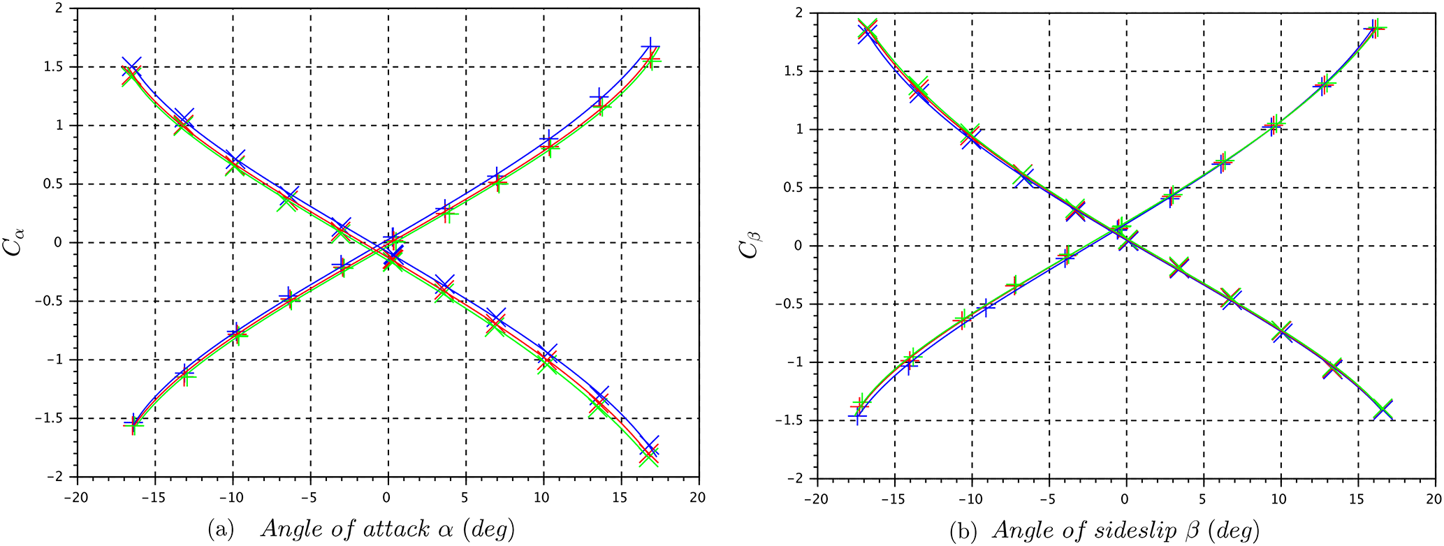
Figure 3 (a) Calibration coefficients C_α for the calculation of the angle of attack α (INS pitch angles as a reference) at different wind tunnel velocities (blue: 15 m s⁻¹; red: 20 m s⁻¹; green: 25 m s⁻¹). The positive slope corresponds to the probe in standard orientation (+ markers). The negative slope corresponds to the probe in inverted orientation (x markers). (b) Calibration coefficients C_β for the calculation of the angle of sidesplit β (INS yaw angles as a reference) at different wind tunnel velocities (blue: 15 m s⁻¹; red: 20 m s⁻¹; green: 25 m s⁻¹). The positive slope corresponds to the probe in standard orientation (+ markers). The negative slope corresponds to the probe in inverted orientation (x markers).

3 Calibration of the five-hole probe

The calibration of the five-hole probe is based on a method described in Wildmann et al. (2014) and consists of a series of wind tunnel experiments to characterize the response of the five-hole probe at different angles. The five-hole probe, the pressure sensors, and the INS are installed in the wind tunnel on a two-axis platform with motion in vertical and horizontal planes (Fig. 2). The calibration of the five-hole probe is a two-step process – first calibrating the differential pressure sensors (Pa), then associating the differential pressures in Pa with angles (α and β; degrees) and air speed (V_a; m s⁻¹). The two-axis platform rotates in the pitch axis (motion in the vertical plane) and yaw axis (motion in the horizontal plane), controlled with a LabView program (Fig. 2). The amplitude of pitch and yaw angles varies up to ±15^∘ to simulate the largest envelope of expected flight conditions. In the wind tunnel, the angle of attack α (five-hole probe) and the pitch angle θ (INS) are, by definition, the same for a well-aligned system, as for the angle of sideslip β (five-hole probe) and the yaw angle ψ (INS). The INS is used as a reference angle measurement between the five-hole probe and the airflow in the wind tunnel. The determination of α, β, and V_a from the five-hole probe depends on four coefficients C_α, C_β, and C_q for the dynamic pressure and C_s for the static pressure (Wildmann et al., 2014; Treaster and Yocum, 1978). To account for offsets in the alignment between the five-hole probe, INS, and wind tunnel, experiments are performed with the probe in the standard orientation shown in Fig. 1, with roll angle equal to 0^∘ (+ markers in Fig. 3), and the probe in inverted orientation for the roll angle equal to 180^∘ (x markers in Fig. 3). Likewise, the same procedure is followed by rotating the five-hole probe by ±90^∘ to determine the offset in the horizontal plane for β. INS angles and ratios of differential pressure sensors are recorded for platform positions between ±15^∘ for three air speeds in the wind tunnel. Figure 3 shows that calibration coefficients are within instrument uncertainty for air speed between 15 and 25 m s⁻¹, and the calibration shows a nearly linear relationship when the probe is within ±10^∘. A systematic offset of 7 % has been found between the calculation of V_a (five-hole probe) and the wind tunnel air speed. The 1σ uncertainty in V_a determined by the five-hole probe is 0.1 m s⁻¹.

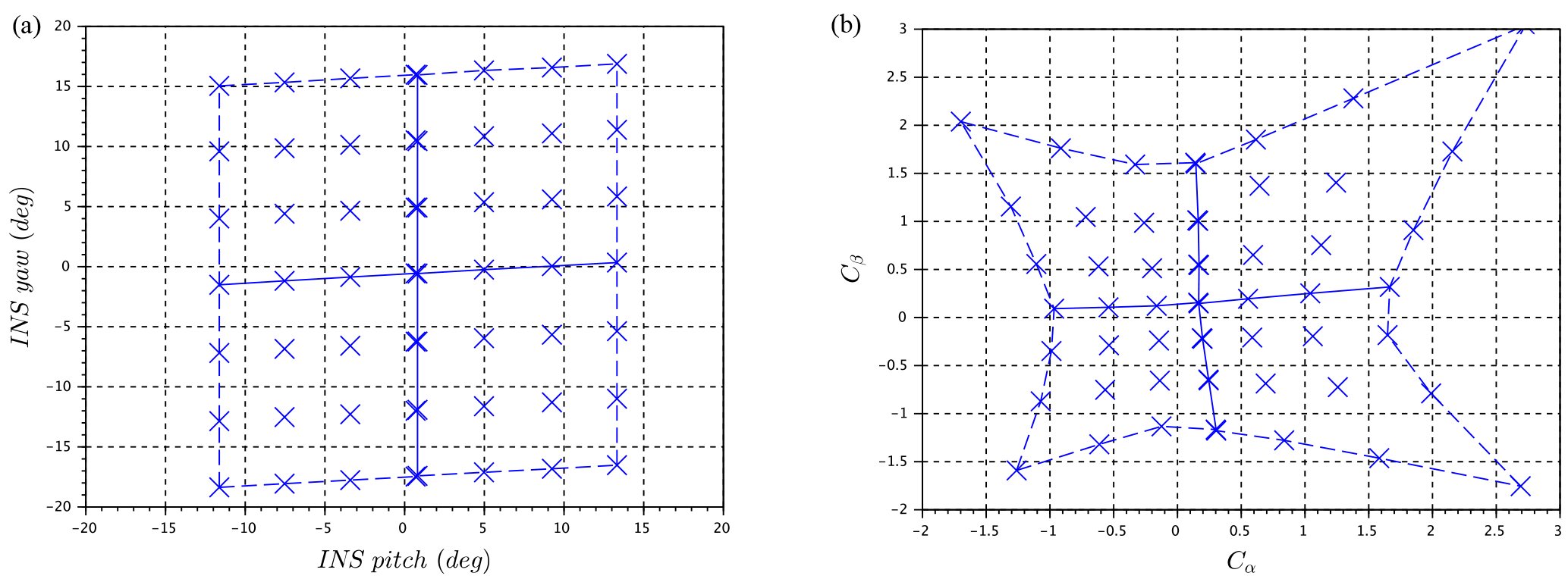
Figure 4 (a) Variation by step of pitch and yaw angles of the two-axis platform in wind tunnel (air speed 15 m s⁻¹). (b) Corresponding C_α and C_β of the five-hole probe to steps of the platform.

To extend the measurements beyond the single-axis of motion described previously, the pitch and yaw angles of the two-axis platform are varied concurrently (Fig. 4a), and the corresponding differential pressure coefficients C_α and C_β are measured (Fig. 4b). This yields a matrix relating the probe's response to the relative vertical (α) and horizontal (β) winds (Fig. 4). The grid in Fig. 4a illustrates the discrete 5^∘ steps in pitch and yaw angles to create a 5×5 calibration matrix for a constant wind speed of 15 m s⁻¹. Similar results are also shown in Wildmann et al. (2014). The horizontal angular bias in Fig. 4 is due to a 3^∘ roll angle in the mounting of the two-axis platform in the wind tunnel. The asymmetry in the calibration matrix (i.e., higher degree of non-linearity on the right side of Fig. 4b) results from a discrepancy in the alignment of the five-hole probe relative to the wind tunnel air flow. The offset between the two-axis platform and the INS is also visible as the grid in Fig. 4a is not centered on 0 (also called the zero-angle offset). The calibration coefficients show a nearly linear relationship for C_α and C_β between values of ±0.7, which corresponds to α and β within ±10^∘ (Fig. 4).

3.1 Experimental error analysis on vertical wind velocity

The performance of the five-hole probe–INS pair is verified by using a dynamic platform to generate motion in the controlled environment of the wind tunnel. The wind tunnel provides a laminar flow; thus vertical wind velocity is, by definition, zero even when the two-axis platform is in motion. Therefore, the response of the five-hole probe can be validated in the wind tunnel by controlling the amplitude (up to ±15^∘) and the angular rate of change (up to 22^∘ s⁻¹) of the platform in the vertical (pitch) axis. As expected, the estimates of vertical wind velocity, w, in the wind tunnel are close to zero. The 1σ standard deviation of w increases with the angular rate of change of the platform (Fig. 5), which seems to be related to a lag in the INS's Kalman filtering process. Under the flight conditions reported in this work, the pitch angle rate of change rarely exceeds ±10^∘ s⁻¹ during straight-and-level legs, implying the minimum resolution of vertical wind velocity measurement with the five-hole probe–INS system is 0.07 m s⁻¹. The uncertainties in w increase when accounting for all parameters, as shown in the next section.

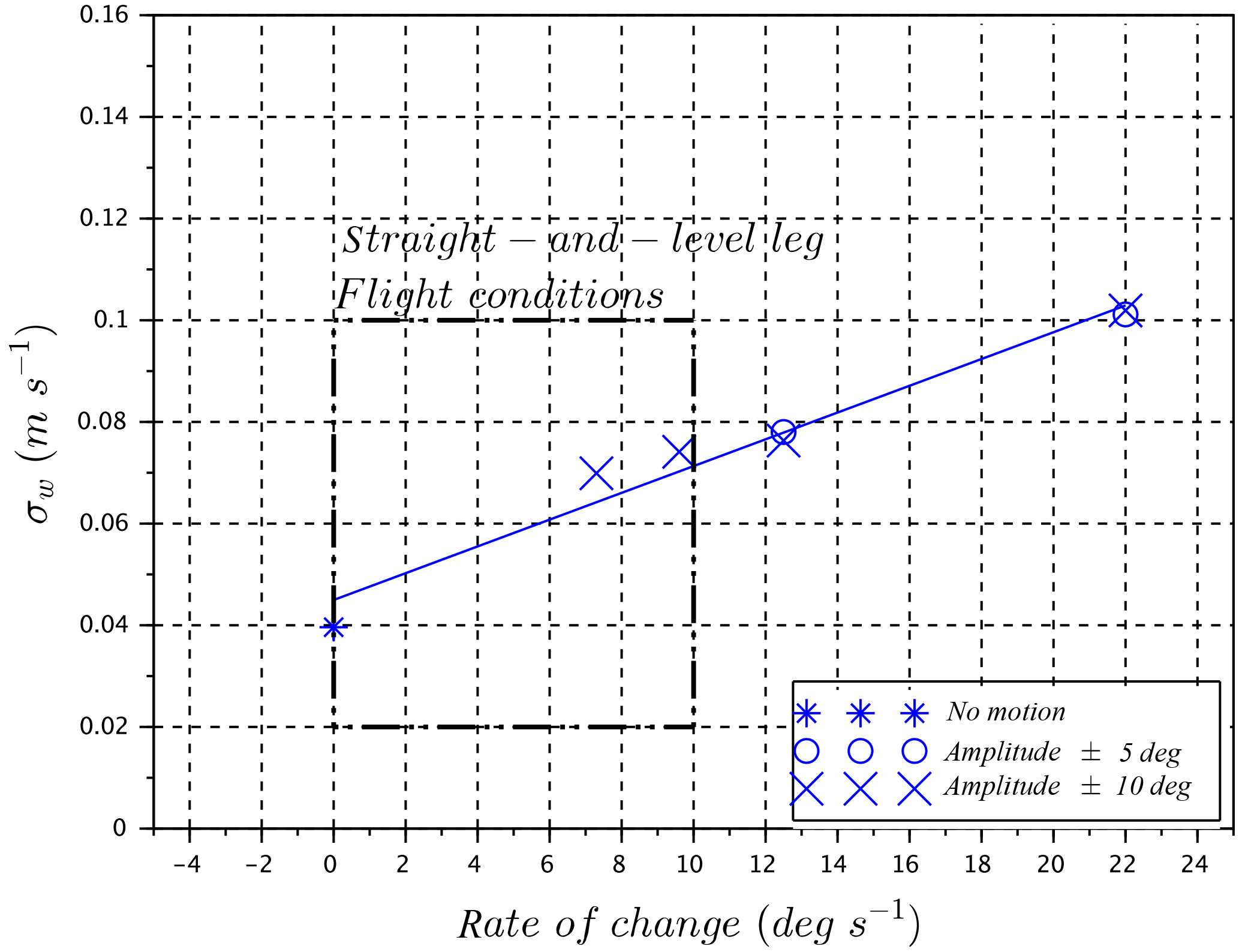
Figure 5 Standard deviation of vertical wind velocity w for each rate of change of the pitch angles on the two-axis platform. For the flight along straight-and-level legs, the rate of change does not exceed 10^∘ s⁻¹.

3.2 Gaussian error propagation on vertical wind velocity

To measure vertical wind velocity of a cloud field, the RPA flies straight-and-level legs at a prescribed altitude. Results from such flight legs show that pitch and roll angles are almost always less than 10^∘ with a rate of change within ±10^∘ s⁻¹, as mentioned in the previous section. In such conditions, the five-hole probe response lies in the quasi-linear regime of the calibration coefficients (Fig. 4), and the small-angle approximations accurately represent the full set of wind equations (Lenschow and Spyers-Duran, 1989). Therefore, the small-angle approximation for the vertical wind velocity equation is used to conduct an uncertainty analysis on w:

$$\begin{array}{}\text{(1)}& {\displaystyle }w=-V_{\mathrm{a}}\sin (\mathit{\theta }-\mathit{\alpha })+V_z,\end{array}$$

with V_a the air speed, θ the pitch angle, α the angle of attack, and V_z the vertical RPA speed. The method used to determine the Gaussian error propagation is similar to the uncertainty analysis conducted in Garman et al. (2006). Here, we present the contribution of each component in Eq. (1) (i.e., angle of attack, air speed, pitch, and vertical RPA speed) to the uncertainty in w. The 1σ uncertainty related to the vertical wind velocity is

$$\begin{array}{ll}{\displaystyle }& {\displaystyle }{\mathit{\sigma }}_{\mathrm{w}}=\\ \text{(2)}& {\displaystyle }& {\displaystyle }\sqrt{{\left({\displaystyle \frac{\partial w}{\partial \mathit{\alpha }}}{\mathit{\sigma }}_{\mathit{\alpha }}\right)}^{\mathrm{2}}+{\left({\displaystyle \frac{\partial w}{\partial V_{\mathrm{a}}}}{\mathit{\sigma }}_{V_{\mathrm{a}}}\right)}^{\mathrm{2}}+{\left({\displaystyle \frac{\partial w}{\partial \mathit{\theta }}}{\mathit{\sigma }}_{\mathit{\theta }}\right)}^{\mathrm{2}}+{\left({\displaystyle \frac{\partial w}{\partial V_z}}{\mathit{\sigma }}_{V_z}\right)}^{\mathrm{2}}}\end{array}$$

where ${\mathit{\sigma }}_{V_{\mathrm{a}}}$ is 0.1 m s⁻¹ (from wind tunnel measurements), σ_θ is 0.25^∘, and ${\mathit{\sigma }}_{V_z}$ is 0.1 m s⁻¹ (both provided by the INS manufacturer). The uncertainties are summarized in Table 1. The error propagation is conducted for α based on C_α in the linear regime (with the slope a_α and the intersect b_α):

$$\begin{array}{}\text{(3)}& {\displaystyle }\mathit{\alpha }=a_{\mathit{\alpha }}{C}_{\mathit{\alpha }}+b_{\mathit{\alpha }}\text{and}{C}_{\mathit{\alpha }}={\displaystyle \frac{\mathrm{\Delta }(P_{\mathrm{4}}-P_{\mathrm{5}})}{\mathrm{\Delta }(P_{\mathrm{1}}-P_{\mathrm{6}})-\mathrm{\Delta }P}},\end{array}$$

with $\mathrm{\Delta }P=\frac{\mathrm{1}}{\mathrm{4}}\left(\right|\mathrm{\Delta }(P_{\mathrm{4}}-P_{\mathrm{5}})|+|\mathrm{\Delta }(P_{\mathrm{2}}-P_{\mathrm{3}})\left|\right)$, Δ(P₄−P₅) the differential pressure between holes 4 and 5, Δ(P₂−P₃) the differential pressure between holes 2 and 3, and Δ(P₁−P₆) the differential pressure between holes 1 and 6 (Fig. 1a). Error propagation of Eq. (3) leads to

$$\begin{array}{}\text{(4)}& {\displaystyle }{\mathit{\sigma }}_{\mathit{\alpha }}=a_{\mathit{\alpha }}{\mathit{\sigma }}_{C_{\mathit{\alpha }}}\end{array}$$

and, as C_α is calculated based on the differential pressures measured by the five-hole probe,

$$\begin{array}{ll}\text{(5)}& {\displaystyle }& {\displaystyle }{\mathit{\sigma }}_{C_{\mathit{\alpha }}}={\displaystyle }& {\displaystyle }\sqrt{{\left({\displaystyle \frac{\partial C_{\mathit{\alpha }}}{\partial \mathrm{\Delta }(P_{\mathrm{4}}-P_{\mathrm{5}})}}{\mathit{\sigma }}_{\mathrm{\Delta }(P_{\mathrm{4}}-P_{\mathrm{5}})}\right)}^{\mathrm{2}}}+\\ {\displaystyle }& {\displaystyle }\stackrel{\mathrm{‾}}{{\left({\displaystyle \frac{\partial C_{\mathit{\alpha }}}{\partial \mathrm{\Delta }(P_{\mathrm{2}}-P_{\mathrm{3}})}}{\mathit{\sigma }}_{\mathrm{\Delta }(P_{\mathrm{2}}-P_{\mathrm{3}})}\right)}^{\mathrm{2}}+{\left({\displaystyle \frac{\partial C_{\mathit{\alpha }}}{\partial \mathrm{\Delta }(P_{\mathrm{1}}-P_{\mathrm{6}})}}{\mathit{\sigma }}_{\mathrm{\Delta }(P_{\mathrm{1}}-P_{\mathrm{6}})}\right)}^{\mathrm{2}}}.\end{array}$$

Table 1 Uncertainty (1σ) associated with parameters from five-hole probe (5HP) and inertial navigation system (INS) for the calculation of error associated with the vertical wind velocity w.

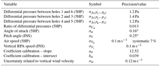
The analysis presented here results in σ_w=0.12 m s⁻¹, which is similar to the uncertainty in w based on the wind tunnel measurements (from Sect. 3.1) and comparable to the results reported by other studies cited in the introduction.

4 Comparison of vertical winds from RPA and sonic anemometers

The measurements of vertical wind velocity on an RPA were compared to sonic anemometers (Campbell CSAT3 3-D Sonic Anemometer) under calm wind conditions at Centre de Recherches Atmosphériques (CRA), which is an instrumented site of the Pyrenean Platform of Observation of the Atmosphere (P2OA), near Lannemezan, France. The purpose of the comparison is (1) to assess the performance of the RPA measurement of updraft by comparing power spectral density (PSD) and vertical wind w distributions measured by sonic anemometers and (2) to calculate TKE used to study boundary layer dynamics and compare with previous studies. Table 2 summarizes flight and wind conditions encountered during these validation experiments. The sonic anemometers are installed on a meteorological mast at 30 m a.g.l. (meters above ground level) and 60 m a.g.l. as part of permanent installations at the CRA. During the experiment, the RPA flew straight N–S and E–W legs in the vicinity of the mast at 60 m a.g.l. The leg length was 1600 m and the duration of flights was approximately 1.5 h. A total of five flights were conducted in different meteorological conditions: a series of three flights were conducted on 15 October 2015 at different times of the day, one flight was conducted in the morning on 20 May 2016, and the last flight was conducted in the afternoon on 7 July 2016 (Table 2). While all flights were conducted in low wind conditions (wind speed less than 4 m s⁻¹), the turbulent conditions differed from one flight to another. The roll angle exceeded 10^∘ less than 1 % of the time, except during flight 4 when roll exceeded 10^∘ 2 % of the time. The pitch angle never exceeded 10^∘, except when approaching stall speed and, even then, only exceeded 10^∘ less than 0.1 % of the time.

Table 2 Description of flights conducted at CRA, Lannemezan, France.

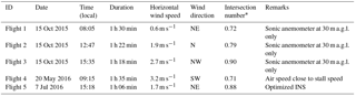
^* Intersection number described in Sect. 4.3.

4.1 Power spectral density functions

To assess the performance of the RPA measurements of atmospheric wind, PSD functions for each of the three wind components of the RPA are compared to PSDs from sonic anemometers. The PSDs of the wind velocities from RPA and sonic anemometers generally follow the $-\mathrm{5}/\mathrm{3}$ slope from the Kolmogorov law as expected (Fig. 6). The PSDs for flights 1, 2, and 3 are averaged to illustrate the probe–INS performance prior to a magnetometer calibration and revised Kalman filtering of the INS (flight 5). During flight 4, the RPA experienced excess motion due to an air speed close to stall speed, which degraded the wind measurements; consequently, results from flight 4 are not included in the analysis. For flights 1, 2, and 3 (prior to reconfiguring the INS), discrepancies in the PSD energy level are visible at 10 ⁻¹ Hz particularly on the u component (Fig. 6b). The bump in the u component at 10⁻¹ Hz is related to the uncertainty in the INS heading measurement, which impacts the horizontal wind calculation, particularly the transversal wind component (the wind component perpendicular to RPA heading). Based on the reverse-heading maneuvers, the uncertainty in horizontal winds is estimated to be within ±1.1 m s⁻¹. After reconfiguring the INS, a notable improvement in PSDs of all three wind components (particularly u component; transversal wind) was observed (Fig. 6; blue lines). The improvement in INS performance clearly demonstrates the importance of precise INS filtering and heading measurements.

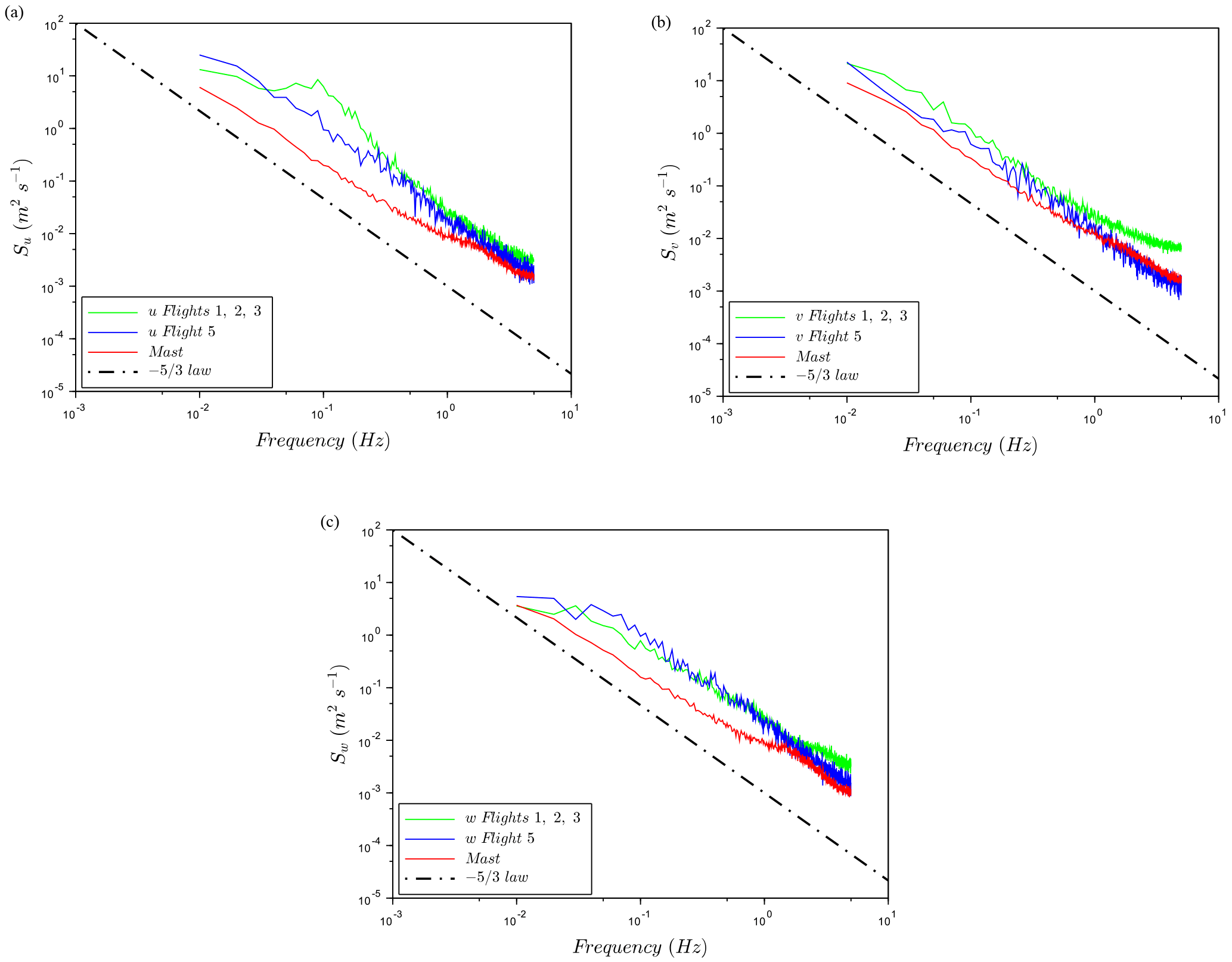
Figure 6 Comparison of averaged PSDs from sonic anemometers (mast: red) and RPA wind measurements averaged for flights 1, 2 and 3 (green), and flight 5 (blue) after the INS has been optimized. The dashed line represents the $f^{-\mathrm{5}/\mathrm{3}}$ law. (a) Spectral energy S of u-wind component function of frequency, (b) Spectral energy S of v-wind component function of frequency, (c) Spectral energy S of w-wind component function of frequency.

Figure 7 Comparison of averaged PSDs from sonic anemometers (mast: red) and RPA wind measurements averaged for flights 1, 2, 3, and 5 (blue). Spectral energy S of decomposed w-wind component with w = A_w (cyan) + V_z (grey) function of frequency. The dashed line represents the $f^{-\mathrm{5}/\mathrm{3}}$ law.

Nonetheless, the PSDs still show a systematic difference between the energy levels related to wind components from the sonic anemometer and the RPA. For the three wind components calculated from RPA measurements, the energy level of ground speeds obtained from the INS (V_x, V_y, and V_z) are higher than the other terms in wind equations for frequencies less than 0.3 Hz. To assess the origin of the different energy levels, the decomposition of the vertical wind equation w (Lenschow and Spyers-Duran, 1989) is based on the simplified form shown as Eq. 1. PSDs of each component of w, V_z (vertical ground speed) and A_w (defined as $-V_{\mathrm{a}}\sin (\mathit{\theta }-\mathit{\alpha })$), are calculated to assess biases related to the INS (Earth frame) and the five-hole probe (RPA frame). The average results from the RPA flights and the sonic anemometers are presented in Fig. 7. The high energy levels at low frequencies seem to be related to uncertainties (even a drift) associated with the vertical velocity measurement. The higher energy levels do translate to systematically higher TKE values (Sect. 4.2); however, these concerns do not significantly impact the results in ACI studies (Sect. 6).

The relatively high energy levels associated with the PSDs are not unique, yet they have not been adequately explained in the literature. Båserud et al. (2016) and Reuder et al. (2016) reported systematically high energy levels of the vertical wind component from the SUMO compared to sonic anemometers on a mast (also at CRA in Lannemezan, France). The issue of higher energy levels was then to “be further investigated in the future”. Other studies have compared TKE values between RPA platforms and a reference; the TKE is linked to PSD energy levels via the variance of each wind component. For example, Lampert et al. (2016) compare TKE between five-hole probe on the M²AV and sonic anemometers (also on the mast at CRA, Lannemezan) and show higher TKE values associated with the M²AV during the afternoon and the night, which also implies higher energy levels of the PSDs. Canut et al. (2016) also compare five-hole probe measurements of M²AV and manned aircraft (Piper Aztec) to sonic anemometer measurements on a tethered balloon. The TKE measurements from the M²AV compare well to the tethered balloon measurements (which indirectly compare well to the sonic anemometer on the mast); however, the results show that TKE measured from the manned aircraft were biased towards higher TKEs. Thomas et al. (2012) conclude that direct comparisons between the RPA and the sonic anemometer are tenuous in their study as the Manta RPA flew at 520 m a.g.l., while the sonic anemometer was only at 10 m a.g.l. Reineman et al. (2013) is the only study that shows similar vertical wind component PSD between a RPA and a ground-based mast (albeit for a relatively short flight above a flat desert). The main difference between the RPAs listed above and the system described in Reineman et al. (2013) is the INS, as no other group has deployed as precise an INS. Since the energy levels of the PSDs for the configuration presented in this paper, are higher, one cannot calculate divergence or convergence; however, the PSDs from the measurements presented here show slopes approaching the expected $-\mathrm{5}/\mathrm{3}$ Kolmogorov regime and the RPA observations reproduce trends in TKE over a range of meteorological conditions. There is certainly more work that needs to be done to improve the turbulence measurements – particularly by improving the INS measurements.

4.2 Turbulent kinetic energy

In the atmospheric boundary layer, the TKE quantifies the intensity of turbulence, which controls mixing of the atmosphere (Wyngaard and Coté, 1971; Lenschow, 1974). TKE is defined as

$$\begin{array}{}\text{(6)}& \mathrm{TKE}={\displaystyle \frac{\mathrm{1}}{\mathrm{2}}}\left({{\mathit{\sigma }}_u}^{\mathrm{2}}+{{\mathit{\sigma }}_{\mathrm{v}}}^{\mathrm{2}}+{{\mathit{\sigma }}_{\mathrm{w}}}^{\mathrm{2}}\right),\end{array}$$

with ${{\mathit{\sigma }}_u}^{\mathrm{2}}$ as the variance of E–W wind, ${{\mathit{\sigma }}_{\mathrm{v}}}^{\mathrm{2}}$ as the variance of N–S wind, and ${{\mathit{\sigma }}_{\mathrm{w}}}^{\mathrm{2}}$ as the variance of vertical wind. To assess TKE values between the wind-RPA (TKE_RPA) and the sonic anemometers on the mast (TKE_mast), we compare different horizontal atmospheric length scales. As the length of each RPA leg is 1600 m, multiples of these legs are chosen for comparison with the sonic anemometers (i.e., 800, 1600, 3200, 4800, 6400 m). The averaging time necessary for the sonic anemometers to record an air mass traveling an equivalent length is calculated using the observed horizontal wind speed and temporally centered with respect to the RPA leg. Mast observations at 30 or 60 m a.g.l. are selected based on data availability (Table 2). Figure 8 clearly shows significant differences between mast-based ${{\mathit{\sigma }}_u}^{\mathrm{2}}$ (E–W wind component) and ${{\mathit{\sigma }}_{\mathrm{v}}}^{\mathrm{2}}$ (N–S wind component) at different altitudes and length scales. Such differences, particularly at 30 m a.g.l., are related to surface topography (e.g., terrain, nearby trees and fields). Meanwhile, Fig. 8 confirms that ${{\mathit{\sigma }}_u}^{\mathrm{2}}$ and ${{\mathit{\sigma }}_{\mathrm{v}}}^{\mathrm{2}}$ are similar at 60 m a.g.l. (i.e., isotropy in the N–S and E–W directions), which can be used to assess the performance of the five-hole probe–INS on the RPA. Results show that TKE_RPA are initially higher than TKE_mast (open diamond markers in Fig. 9), as u (the transversal wind component) shows higher variances than v (as described in Sect. 4.1). Applying the observed isotropy shown in Fig. 8 (${\mathit{\sigma }}_{u,\mathrm{RPA}}^{\mathrm{2}}={\mathit{\sigma }}_{v,\mathrm{RPA}}^{\mathrm{2}}$ at 60 m a.g.l.) for the RPA observations, the comparison of TKE_RPA and TKE_mast improves (Fig. 9; solid diamond markers) by replacing ${{\mathit{\sigma }}_u}^{\mathrm{2}}$ by ${{\mathit{\sigma }}_{\mathrm{v}}}^{\mathrm{2}}$ in the calculation of TKE_RPA. We note, however, the isotropic conditions are not always satisfied (i.e., longitudinal wind rolls affecting crosswind fluxes reported in Reineman et al., 2016). Consequently, a RPA flight strategy, such as parallel and cross-wind legs, is essential in identifying isotropic conditions and measurement errors associated with the five-hole probe–INS system.

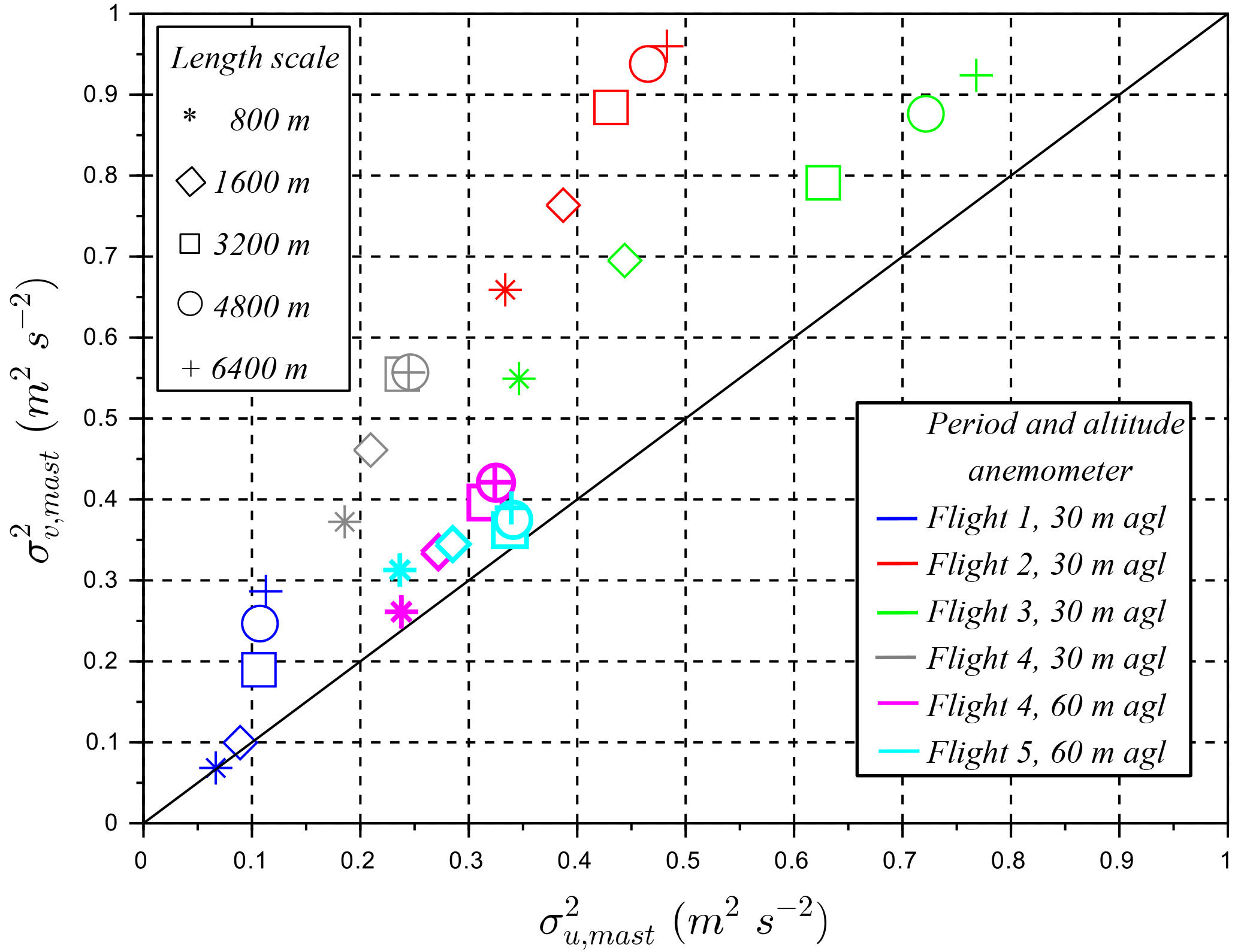
Figure 8 Comparison of TKE_RPA and TKE_mast. Open diamonds TKE_RPA are calculated with the three wind variances of RPA, solid diamonds are obtained with an isotropy assumption ${\mathit{\sigma }}_{u,\mathrm{RPA}}^{\mathrm{2}}={\mathit{\sigma }}_{v,\mathrm{RPA}}^{\mathrm{2}}$ observed at 60 m a.g.l. by the sonic anemometer in Fig. 8. The uncertainty bars correspond to 1σ, using all the legs during the RPA flights and using each length scale from 800 to 6400 m for the sonic anemometers.

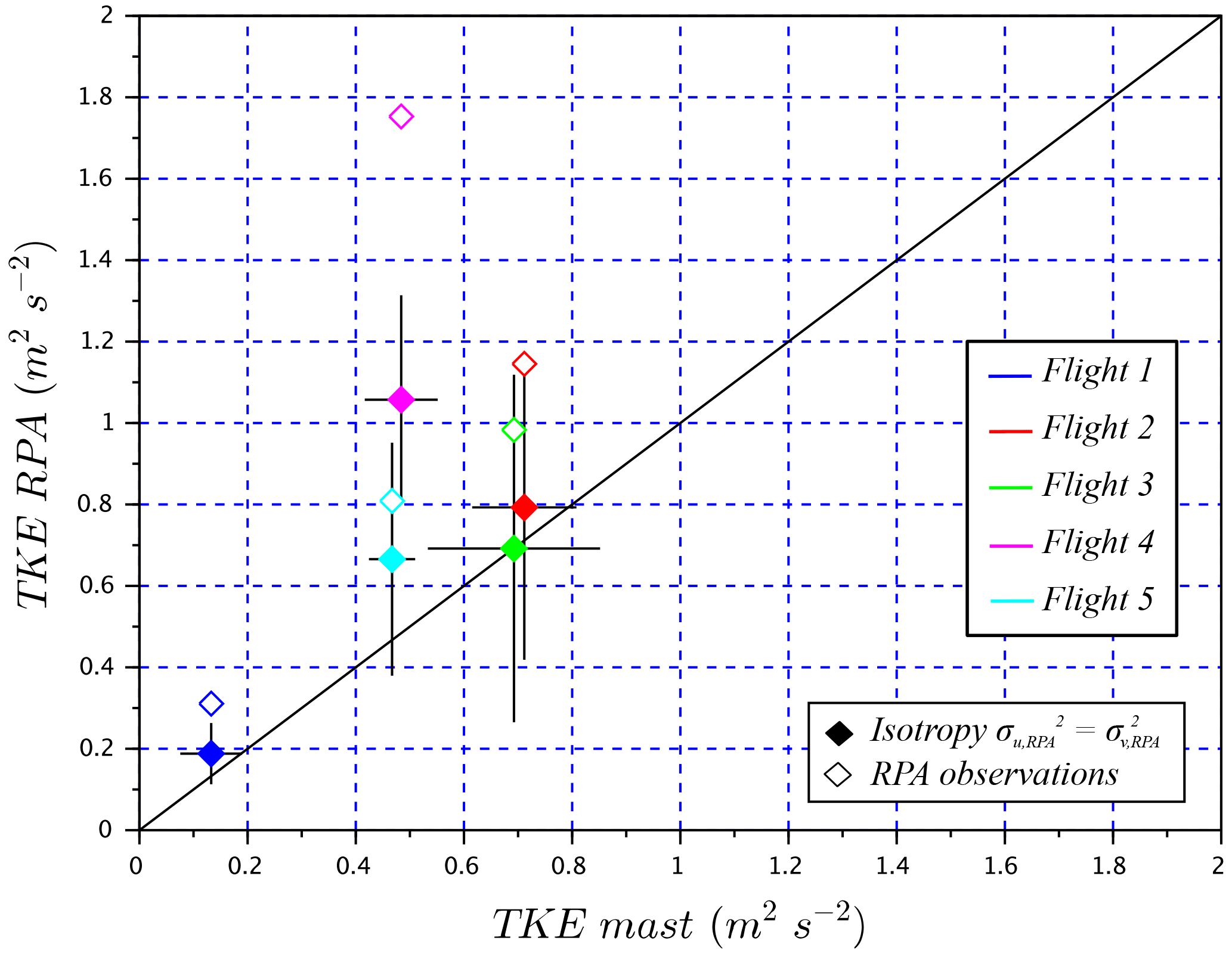
Figure 9 Comparison of variances ${\mathit{\sigma }}_{u,\mathrm{mast}}^{\mathrm{2}}$ and ${\mathit{\sigma }}_{v,\mathrm{mast}}^{\mathrm{2}}$ from the sonic anemometers for the associated flight periods and length scales.

As mentioned in Sect. 4.1, studies that report TKE have been published that compare the SUMO and M²AV to the sonic anemometer at CRA, Lannemezan (Båserud et al., 2016; Lampert et al., 2016). The reported values of TKE from both of these studies are within 50 % of TKE from the sonic anemometer. Canut et al. (2016) also show a relatively good agreement of TKE between a tethered balloon, the M²AV, and the manned aircraft with a correlation coefficient R²=0.88. In this study, for the comparison between the wind-RPA and sonic anemometers (Fig. 9), the slope of the linear regression for the RPA observations is 1.32 (R²=0.97) and improves to 0.95 (R²=0.91) with the isotropy assumption (${\mathit{\sigma }}_{u,\mathrm{RPA}}^{\mathrm{2}}={\mathit{\sigma }}_{v,\mathrm{RPA}}^{\mathrm{2}}$). Flight 4 is not included in this analysis because of known issues related to flight performance. These results suggest that improving the measurement of horizontal winds and reducing biases in the horizontal components of the variances may be achieved by (1) improvement of the INS heading measurement (also noted in Elston et al., 2015) and (2) verified with a cross-leg flight plan (i.e., orthogonal legs).

4.3 Vertical wind velocity distributions

To compare vertical wind from the RPA to the sonic anemometer, angle of attack α and pitch angle θ are re-centered such that average vertical velocity w is 0 m s⁻¹ over the time of the flight. This step is needed because the alignment of the five-hole probe relative to the Earth's frame may change with meteorological conditions (such as wind speed) and flight parameters (such as air speed and nominal pitch angles). The re-centering step of the five-hole probe on the RPA is further justified by results from the sonic anemometers on the mast, which also show an average vertical velocity approaching 0 m s⁻¹ over the duration of the flight. Distributions of vertical wind velocities from the RPA and sonic anemometer at 60 m a.g.l. are compared, and the intersection method is used to quantify the agreement between the distributions. An example of the vertical wind distributions are shown in Fig. 10 for flight 5. The calculation of the intersection number is obtained from $\sum _{i=\mathrm{1}}^{N}min\left(I_i,M_i\right)$ with I and M as the normalized distributions to be compared, and N as the total number of bins. For an exact match, the intersection method result is unity; for a complete mismatch, the result is zero. Table 2 summarizes the intersection numbers between the RPA and sonic anemometer vertical wind distributions for the five flights. The intersection numbers between RPA and anemometer vertical wind distributions are higher than 70 %. As expected, this value is lower during flight 4.

Figure 10 Distribution functions of vertical wind w for RPA and sonic anemometer at 60 m a.g.l. measurements, flight 5. The vertical bars represent the uncertainty (σ_w=0.12 m s⁻¹) associated with RPA vertical wind measurements.

5 Comparison of vertical wind velocities from RPA and cloud radar

A BACCHUS field campaign took place at the Mace Head Atmospheric Research Station on the west coast of Galway, Ireland, in August 2015. The purpose was to study ACIs, linking ground-based and satellite observations using RPAS (Sanchez et al., 2017). Among the four instrumented RPAs which flew at Mace Head, the wind-RPA was equipped with a five-hole probe and an INS to obtain vertical wind velocities, as well as upward- and downward-facing pyranometers to identify cloud sampling periods. During the campaign, we concentrated on measurements of vertical wind velocity near cloud base or within clouds to study ACIs. After identifying the cloud base from the ceilometer or based on a vertical profile of an earlier flight, the wind-RPA was sent to an altitude close to cloud base, flying 6 km long straight-and-level legs. Horizontal wind speeds varied from 6 to 12 m s⁻¹ from the west during the case studies presented here. During this field campaign, the wind-RPA flew in 10 of the 45 scientific flights for a total of 15 h. Of the 10 flights with the wind-RPA, three flights contained a complete set of observations (vertical winds, pyranometers, and cloud radar measurements). The other flights were not selected for a number of reasons: water in the five-hole probe (two flights), insufficient number of cloud radar data for comparison (two flights), no cloud (one flight), no pyranometer data to identify clouds (one flight), and aborted mission due to strong winds (>15 m s⁻¹, one flight). In this section, we focus on three flights with the wind-RPA (Table 3), in which the vertical wind from the RPA is compared to vertical wind from the cloud radar at Mace Head.

Table 3 Description of BACCHUS case study flights, Mace Head Research Station, Ireland. The intersection number compares vertical wind velocity distributions between RPA and cloud radar.

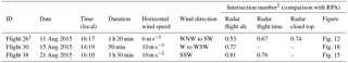
¹ No pyranometer data. ² Intersection number described in Sect. 4.3

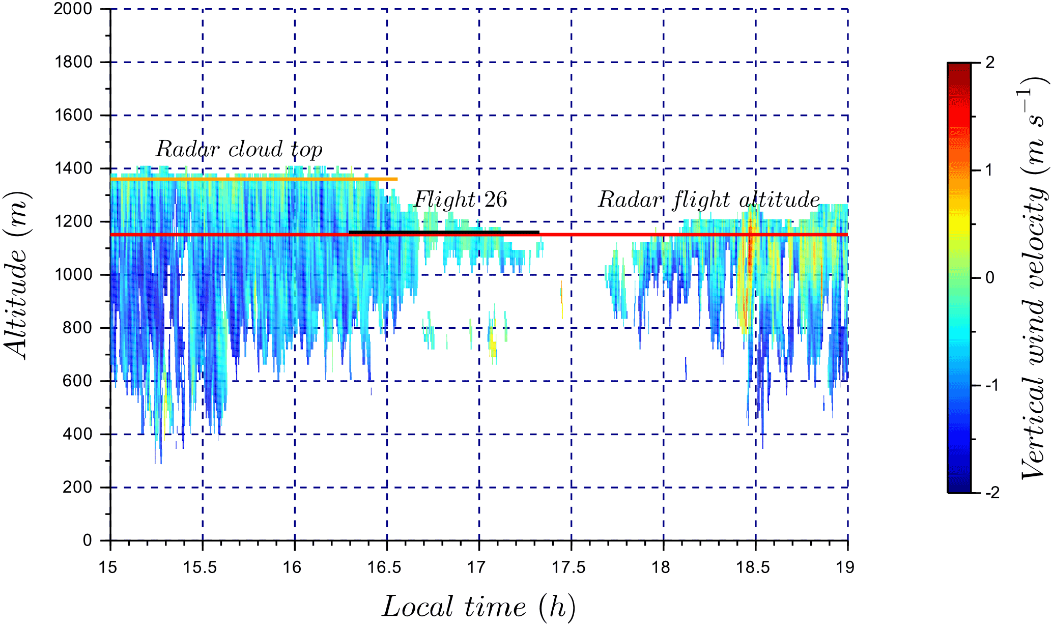
Figure 11 Time series of vertical wind velocity for a stratocumulus deck with light precipitation (flight 26). The color bar represents the cloud radar vertical wind velocity. Flight 26 sampling time is identified by the black segment. The red horizontal line corresponds to radar data at the altitude of the RPA (1160 m a.s.l.), and the orange line corresponds to radar data at cloud top (1360 m a.s.l.). Cloud radar vertical wind velocity at 1160 m a.s.l. and 1360 m a.s.l. are used in Fig. 12 to compare with RPA measurements.

The Doppler cloud radar (cloud radar MIRA-35, METEK, 35.5 GHz, Ka band) at the Mace Head Research Station is adapted to the observation of the cloud structure (Görsdorf et al., 2015). The cloud radar is equipped with a vertically pointed antenna with a polarization filter, a magnetron transmitter, and two receivers for discerning polarized signals. Measurements are available up to 15 km height for a temporal resolution of 10 s. The vertical resolution of the cloud radar is 29 m. In this study, cloud radar data from the cloud top or the RPA flight altitude are selected for the comparison.

While the flight altitude for the wind-RPA was estimated to be near the cloud base, uncertainties in retrieving cloud base height or an evolution in cloud base height related to diurnal cycles of the boundary layer inevitably lead to the RPA flying in the clouds rather than below cloud base. Note that direct comparison of instantaneous data between the RPA and cloud radar is not possible, as the RPA did not fly directly over the cloud radar and did not observe the same air mass. Moreover, the cloud radar reports vertical velocities every 10 s (and only when a cloud is present); therefore, relatively long averaging periods are needed to compare vertical velocity distributions of the cloud radar with RPA observations. In this section, we present selected time series of the cloud radar measurements that represent the state of the atmosphere during the flight; for cases with sufficient cloud cover, we present different averaging periods of the cloud radar (a short period that coincides with the RPA flight and longer periods for better counting statistics). In the present study, normalized vertical wind velocity distributions of the cloud radar serve to validate the RPA results. In addition, the vertical velocity distributions provide insight on different atmospheric states (e.g., in–out of cloud, over water or land).

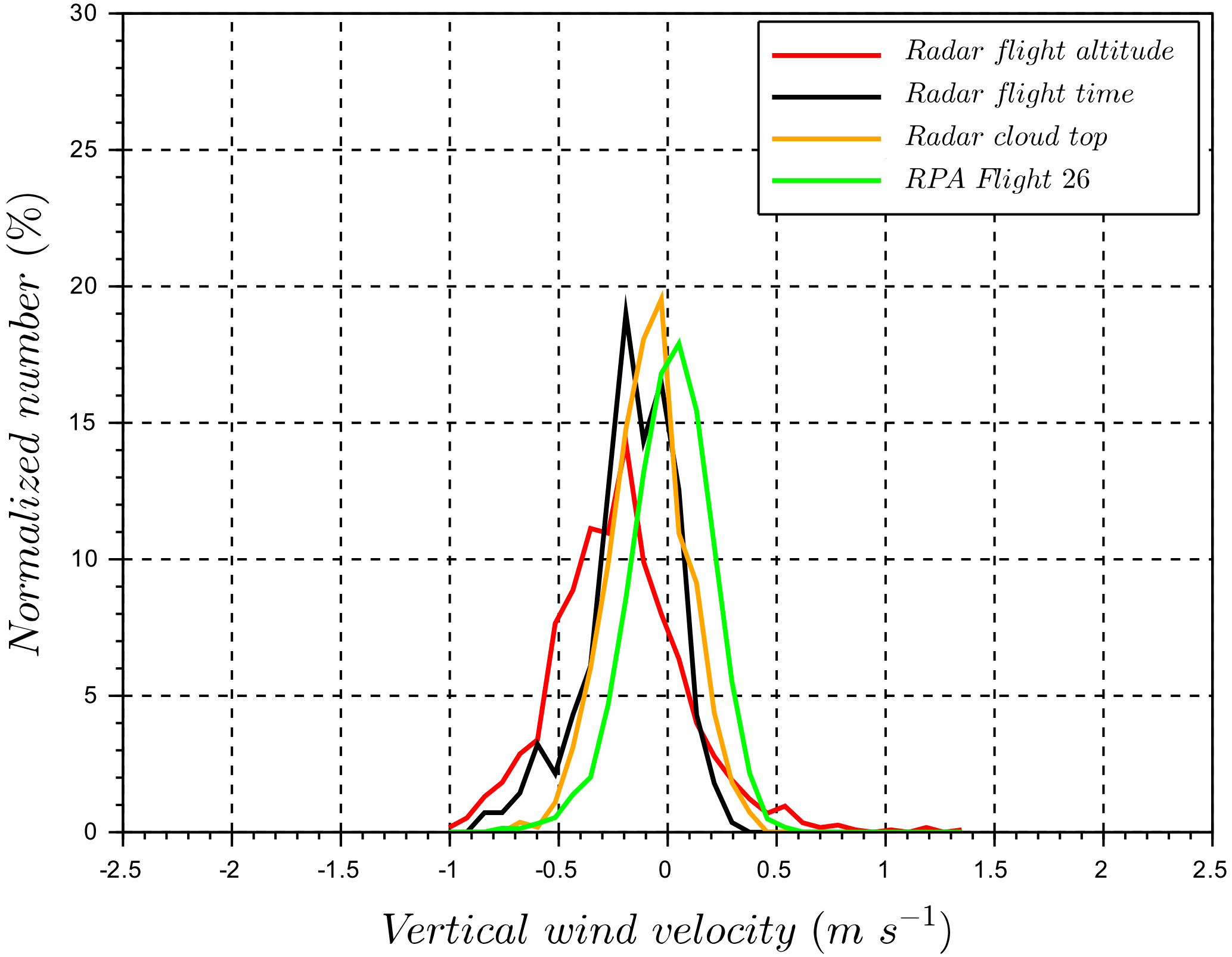
Figure 12 A comparison of vertical wind velocity distributions in a lightly precipitating stratocumulus deck between RPA (1160 m a.s.l.), cloud radar at RPA altitude (1160 m a.s.l.), and cloud radar at cloud top (1360 m a.s.l.). “Radar flight altitude” corresponds to 4 h of cloud radar measurements at the same altitude as the RPA flight. “Radar flight time” corresponds to the cloud radar measurements during the RPA flight period at the same altitude as the RPA. “Radar cloud top” corresponds to cloud radar measurements near the cloud top, which is in the non-precipitating part of the cloud. “RPA flight 26” corresponds to RPA vertical wind measurements during flight 26. Time periods and altitudes are identified in Fig. 11.

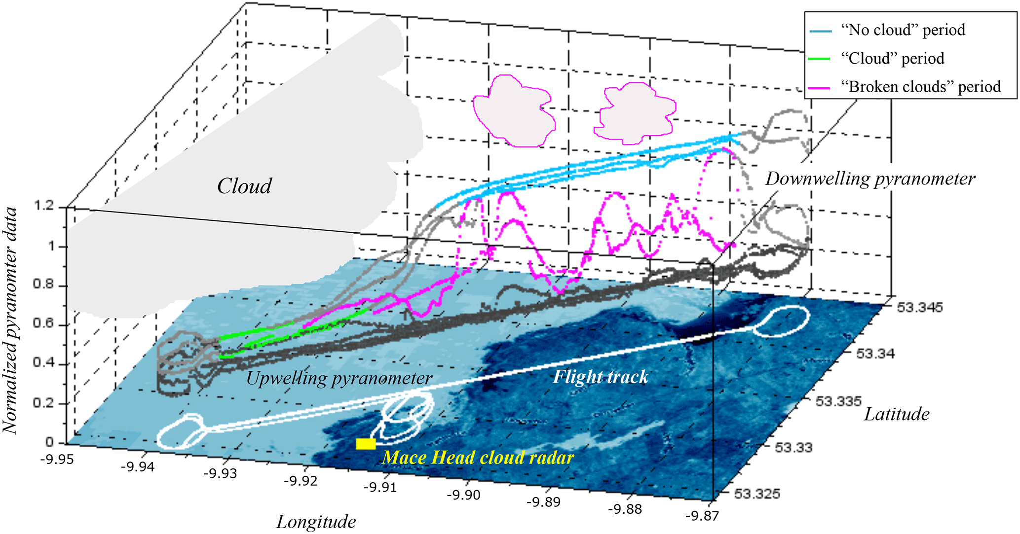
Figure 13 Coastal map and flight tracks for the case study of a convective cloud with changing meteorology (flight 38). Downwelling and upwelling pyranometers data are color-coded based on the three flight periods (“cloud”, “no cloud”, and “broken clouds”). The developing field of broken clouds (magenta contour clouds) appeared during the last two legs. The cloud radar (yellow square) operated at the Mace Head Research Station.

5.1 Stratocumulus deck with light precipitation (flight 26: 11 August 2015)

On 11 August, the sky was covered by a lightly precipitating stratocumulus deck, and the wind-RPA flew at 1160 m a.s.l. (about 100 m above the cloud base). The time series of vertical wind from the cloud radar is presented in Fig. 11, along colored horizontal lines that indicate observation periods of the cloud radar and RPA. Figure 12 presents a comparison of the normalized vertical wind distributions obtained by cloud radar and the RPA measurements. The standard deviation of RPA vertical wind distribution is σ_RPA=0.19 m s⁻¹ (or 0.10 m s⁻¹ if only positive vertical velocities are considered). This result is comparable to the range of vertical wind standard deviations obtained in Lu et al. (2007) for stratocumulus clouds observed off the coast of Monterey, California, in the eastern Pacific ($\mathrm{0.06}<{\mathit{\sigma }}_{\mathrm{w}}<\mathrm{0.29}$ m s⁻¹, for w>0 m s⁻¹ from 11 sampled stratocumulus clouds). In this case study, the presence of falling cloud droplets to an altitude as low as 300 m a.g.l. (Fig. 11) negatively biases the vertical wind distribution retrieved from the cloud radar (Fig. 12). Previous measurements have also shown that precipitation negatively biases cloud radar observations of vertical wind velocities, as the radar indirectly measures vertical wind by using the motion of scatterers (i.e., hydrometeors; Lothon et al., 2005; Bühl et al., 2015). These negative biases in retrieved vertical winds are largely removed by obtaining vertical velocity distributions at the top of the cloud (Bühl et al., 2015). Similar results are obtained for our case study, as the cloud radar is strongly influenced by falling droplets, yet only slightly negatively biased at the cloud top. The intersection method, described in Sect. 4.3, is used to compared the normalized cloud radar vertical wind distributions to those of the RPA (Table 3). The intersection number is 0.53 between cloud radar and observations at the RPA flight altitude. This relatively low match is a result of the negative bias from the precipitating droplets. A much better agreement is found between the cloud radar vertical velocity distribution retrieved at the cloud top (1360 m a.s.l.) and the RPA measurements (intersection number =0.74).

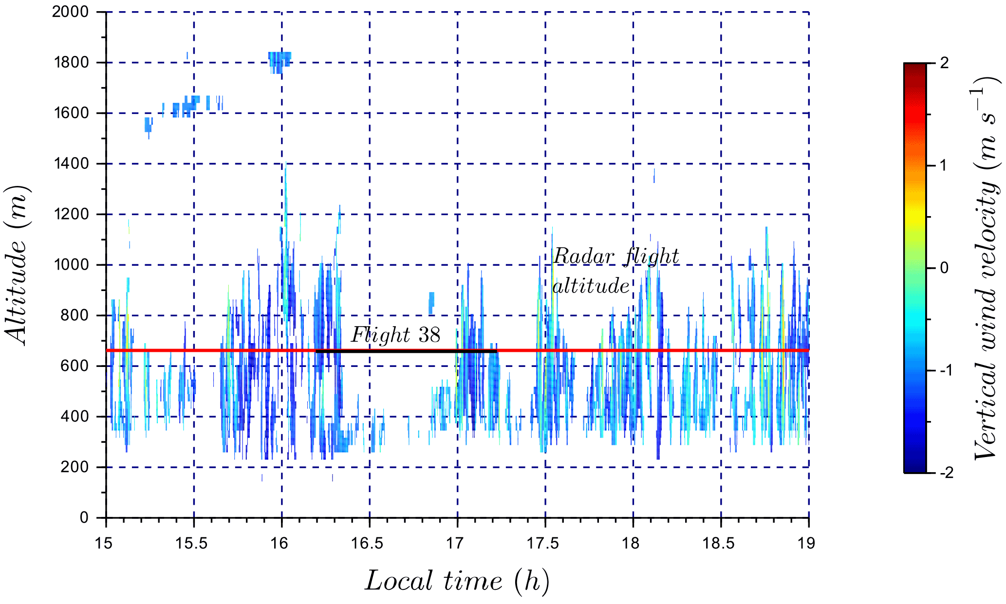
Figure 14 Time series of vertical wind velocity associated with flight 38. The color bar represents the cloud radar vertical wind velocity. Flight 38 sampling time is identified by the black segment. The red horizontal line corresponds to radar data at flight altitude (660 m a.s.l.), used to plot vertical wind velocity distributions in Fig. 15.

5.2 Cloud fields with changing meteorology (flight 38: 21 August 2015)

In this case study, the results from the RPA and cloud radar emphasizes the differences in vertical wind distributions depending on the meteorological conditions related to cloud field. The wind-RPA flew within a cloud above the ocean and in clear sky above land for three legs, after which the local meteorology changed into a formation of developing clouds above land (where a cloudless sky had previously been observed; Fig. 13). The vertical wind velocity distributions are presented using a combination of information shown in a series of figures: downwelling and upwelling pyranometer observations and three periods corresponding to distinct meteorological conditions (Fig. 13); the time series of cloud radar data (Fig. 14); and the vertical wind distributions from the RPA and the cloud radar (Fig. 15). These meteorological periods are defined in Fig. 13 as “cloud” (both pyranometers approach similar values), “no cloud” (downwelling pyranometer is significantly higher than upwelling pyranometer), and a third period associated with a developing field of broken clouds (spatially variable downwelling pyranometer). Based on the pyranometer measurements, we deduce a cloudless sky (cyan) was observed by the RPA above land for the first three legs (Fig. 13). The cloud radar also did not detect clouds above land for the beginning of the flight (Fig. 14). In the meantime, the RPA flew within a cloud above the ocean (Fig. 13, green), which was not observed by the cloud radar. Figure 15 shows that the standard deviation of vertical velocity within the cloud is larger than for clear sky conditions (σ_cloud=0.28 m s⁻¹, σ_{no cloud}=0.17 m s⁻¹) , which highlights the presence of stronger vertical winds in the presence of clouds. During the last two legs of flight 38, the wind-RPA flew through a developing field of broken clouds above land (Fig. 13, magenta), which also appeared in the cloud radar time series and in the satellite image (Fig. 4 in Sanchez et al., 2017). The standard deviation during the “broken cloud” RPA period is larger than the other periods (σ_{broken cloud}=0.46 m s⁻¹), and the shape of vertical wind distributions is similar for both the cloud radar and the RPA (Fig. 15). While not shown here, the vertical wind distributions observed by the cloud radar are similar at cloud base (380 m a.s.l.) and at the flight altitude (660 m a.s.l.), as well as over different lengths of observing periods (1.5 and 4 h). In Table 3, intersection numbers illustrate the relatively close matches (ca. 80 %) in comparing the “broken cloud” RPA period and the cloud radar for 4 h (radar flight altitude) and for 1.5 h (radar flight time). The similar results for the observations of a field of broken clouds independently reinforces RPA and cloud radar observational methods, and the changes in meteorological conditions highlight the ability to identify distinct states of the atmosphere with the RPA.

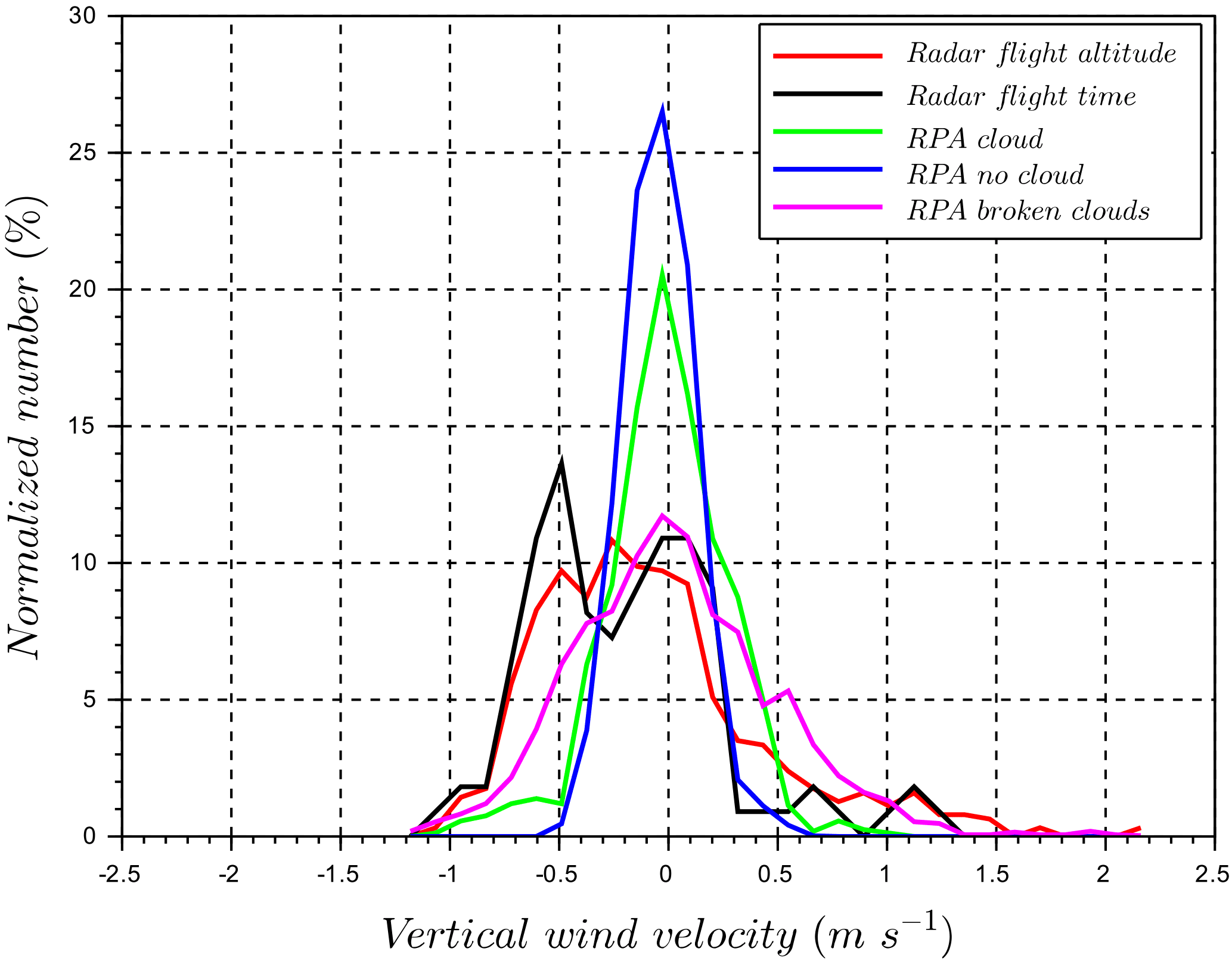
Figure 15 Comparison of vertical wind velocity distributions for RPA and cloud radar for flight 38. “Radar flight altitude” corresponds to 4 h of cloud radar measurements at RPA flight altitude. “Radar flight time” corresponds to the cloud radar measurements during the RPA flight period at the same altitude as the RPA. The time series are defined in Fig. 14. RPA measurements are divided into periods defined in Fig. 13 (“cloud”, “no cloud”, and “broken clouds” periods). The cloud radar detected cloud only for the “broken clouds” period during the RPA flight.

Figure 16 Coastal map and flight tracks for the non-convective cloud case study (flight 30). Downwelling and upwelling pyranometers data are color-coded based on two flight periods, “cloud” and “no cloud” periods. The cloud radar (yellow square) operated at the Mace Head Research Station.

5.3 Fair weather cumulus clouds (flight 30: 15 August 2015)

During flight 30, the cloud field was scattered with small clouds as shown in Fig. 17 by the cloud radar time series. However, the number of data points from the cloud radar during the flight time (black segment) was insufficient to establish a vertical wind distribution, therefore only the cloud radar data for 4 h (red segment) are presented in Fig. 18. The wind-RPA flew through one of these clouds as shown by the pyranometer measurements in Fig. 16. To compare cloud radar and RPA data, vertical winds from the RPA are again divided into “cloud” and “no-cloud” periods based on pyranometer observations. The respective standard deviations for the periods are σ_cloud=0.35 m s⁻¹ and σ_{no cloud}=0.34 m s⁻¹, which are not statistically different. However, the variability between legs is significantly greater in the “no cloud” period (as represented by the envelope in blue dashed lines in Fig. 18) compared to the “cloud” period (envelope in green dashed lines). In Fig. 18, the RPA and cloud radar measurements show similar results during the “cloud” period, with an intersection number equal to 0.76. Kunz and de Leeuw (2000) have observed an upward component in the air flow at the surface from the ocean at the Mace Head Research Station as a result of the terrain. However, systematic differences between the RPA and cloud radar have not been observed for the other case studies, so we cannot quantify the role of surface heating or orography on the cloud radar vertical distributions compared to those of the RPA.

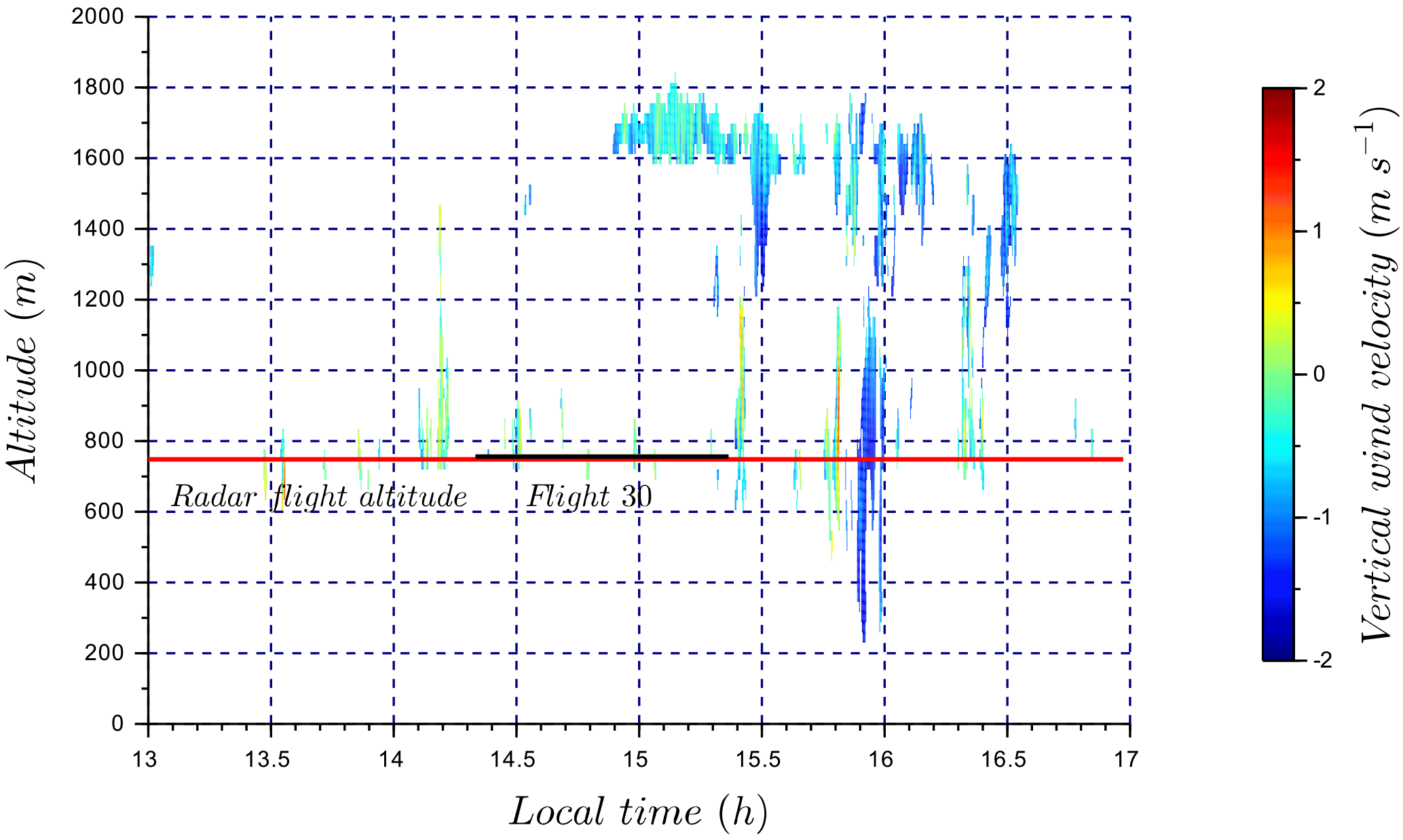
Figure 17 Time series of vertical wind velocity associated with flight 30. The color bar represents the cloud radar vertical wind velocity. Flight 30 sampling time is identified by the black segment. The red horizontal line corresponds to radar data at flight altitude (750 m a.s.l.) used in Fig. 18 to plot vertical wind velocity distribution.

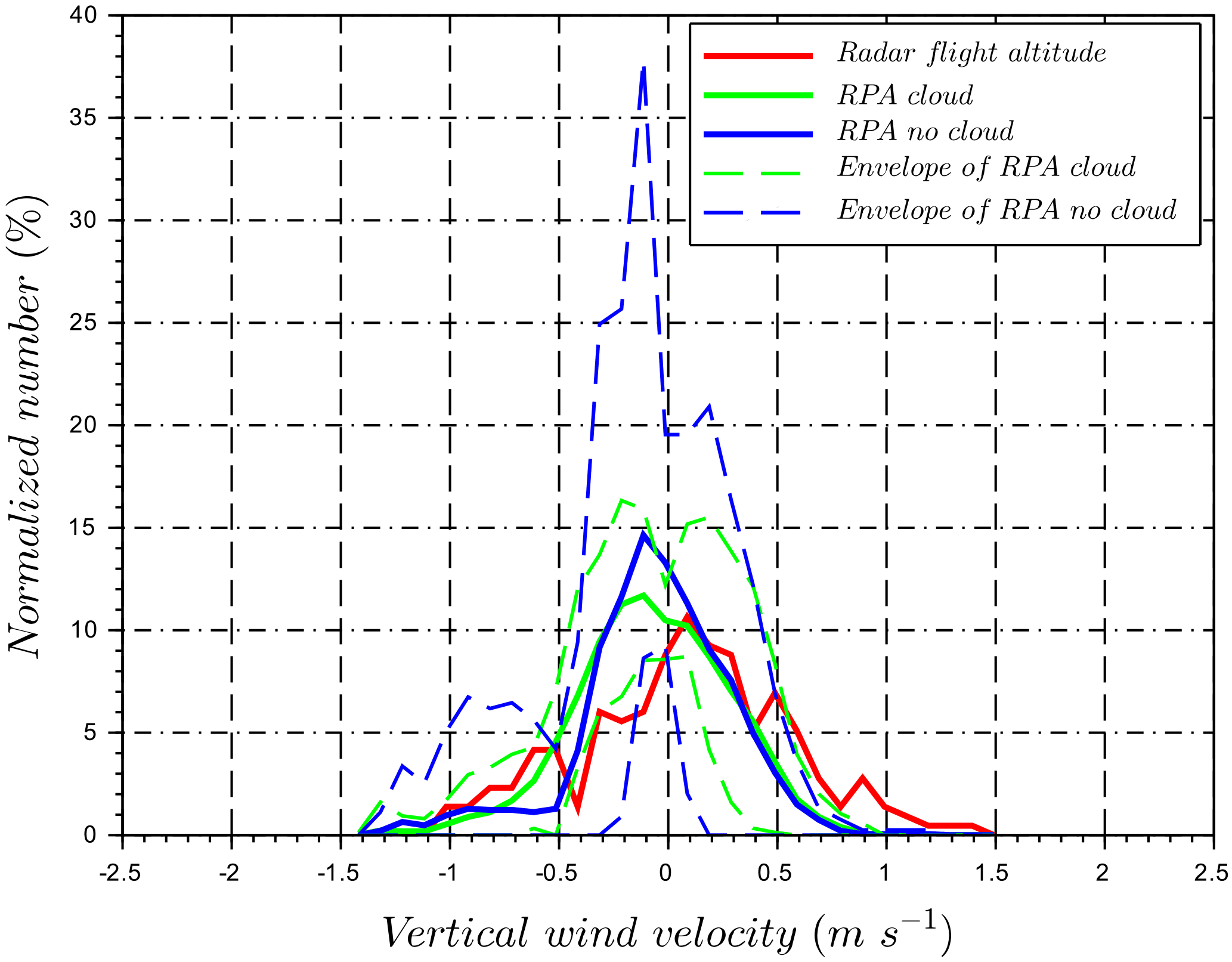
Figure 18 Comparison of normalized vertical wind velocity distributions for RPA during flight 30 and cloud radar at RPA flight altitude (750 m a.s.l.). “Radar flight altitude” period is defined in Fig. 17. RPA measurements are divided into “cloud” and “no cloud” periods. The envelope of each period is plotted based on the minimum and maximum number per bin vertical velocity distributions on a leg-by-leg basis.

6 Sensitivity of vertical winds on aerosol–cloud interactions

To study ACIs, the input parameters for an aerosol–cloud parcel model (ACPM) are obtained from vertical profiles (temperature, relative humidity), straight-and-level legs (updraft), and measurements of cloud condensation nuclei spectra and aerosol size distributions. A weighted ensemble of updraft velocities, based on five-hole probe measurements, is used in the parcel model to simulate the cloud droplet distribution, (Sanchez et al., 2016, 2017). A sensitivity study assesses the impact of the vertical velocity distributions between the RPA and anemometer (Sect. 4) or cloud radar (Sect. 5) on the resulting cloud droplet number concentrations for populations. The sensitivity is equal to $\mathrm{1}/N*dN/dw$ with N the cloud droplet number concentration and dN∕dw the slope of the cloud droplet number / updraft relationships found in Martin et al. (2017) and Ming et al. (2006). The resulting cloud droplet number concentration is more sensitive at low concentrations ($\sim \mathrm{1}/N$) and at low updraft velocities (when dN∕dw is the largest). Based on polluted and clean cases described in Martin et al. (2017), cloud droplet numbers are ca. 100 and 350 cm⁻³, respectively, with relative differences owing to RPA and anemometer/cloud radar updraft velocities within 10 %. While the cloud droplet number concentration simulated with the RPA measurements is systematically higher than from sonic anemometer owing to the broader RPA vertical velocity distributions, a systematic difference in cloud droplet number concentrations is not observed between the RPA and cloud radar. These results suggest that the updraft measurements based on RPA measurements are sufficiently accurate for representing ACIs.

7 Conclusions

The validation of vertical wind measurements in clouds measured by a five-hole probe on a lightweight remotely piloted aircraft (RPA) has been detailed in this study. Atmospheric winds in the Earth's coordinate system are derived using the equations described in Lenschow and Spyers-Duran (1989) with the velocity of the RPA with respect to the Earth (measured by the inertial navigation system, INS), and the velocity of the air with respect to the RPA (measured by the five-hole probe). The attitude angles measured by the INS are used for coordinate system transformation from RPA to the Earth's coordinate system. The five-hole probe has been calibrated in wind tunnel on a two-axis platform to obtain the angle of attack, angle of sideslip, and air speed of the RPA. Motions induced by the dynamic platform in the wind tunnel were effectively removed, thereby validating probe–INS performance. Nonetheless, the rate of the angular rotation of the platform does impact the precision of derived atmospheric winds. The uncertainty associated with the vertical wind measurement w is determined to be 0.12 m s⁻¹ using a Gaussian error propagation analysis (and uncertainty related to horizontal wind is 1.1 m s⁻¹ based on reverse-heading maneuvers). Vertical velocity distributions from the RPA and sonic anemometers show intersection values higher than 70 % in calm wind conditions. Comparisons have also been made between power spectral density (PSD) functions of the sonic anemometer and RPA measurements and demonstrate the impact of optimizing INS heading measurements on the PSD (particularly for the transversal component of wind). The observed isotropy by the sonic anemometer at 60 m a.g.l. is used to improve estimates of turbulent kinetic energy (TKE) obtained from RPA wind measurements. However, orthogonal flight plans must be implemented in order to account for parallel- and cross-wind atmospheric conditions and measurement biases (particularly related to transversal wind components).

Three case studies from a BACCHUS field campaign (at the Mace Head Atmospheric Research Station, Galway, Ireland) validated RPA vertical wind velocities in clouds compared to cloud radar observations. Vertical wind velocity distributions were classified according to the flight periods (e.g., clear sky or cloud), emphasizing the impact of meteorology and the state of the atmosphere on the distribution of vertical wind velocities in the cloud field. For the first case study, a stratocumulus deck covering the sky and light precipitation was observed. Cloud radar vertical wind velocity distribution was negatively biased and cloud base was not distinctly visible due to falling droplets. The wind-RPA provided a centered vertical wind distribution near cloud base, which was similar to cloud radar observations at cloud top (in the non-precipitating region of the cloud). The second case study displayed different meteorological conditions during the flight, which were well distinguished by the wind-RPA, including differences between a developing field of broken clouds, a small convective cloud, and clear sky. In the third case study, similar vertical wind distributions in clouds were observed by the RPA and the cloud radar in fair weather cumulus cloud systems above land and ocean. The vertical velocity distributions, which were encountered for each of the case studies, highlighted the ability of the RPA platform to differentiate the meteorological conditions associated with the cloud systems based on vertical wind measurements.

To estimate the impact of discrepancies in vertical wind distributions on cloud droplet number concentrations, a sensitivity study was conducted to assess the relationship between cloud droplet number concentrations and updraft for different aerosol populations. The difference in vertical wind distributions between RPA and anemometer/cloud radar generally resulted in differences less than 10 %. These results demonstrate that vertical velocity measurements on the RPA are sufficiently accurate to conduct aerosol–cloud closure studies using RPAs.