the Creative Commons Attribution 4.0 License.
the Creative Commons Attribution 4.0 License.
 | 08 May 2018
Instantaneous variance scaling of AIRS thermodynamic profiles using a circular area Monte Carlo approach
Jesse Dorrestijn
Brian H. Kahn
João Teixeira
Fredrick W. Irion
Satellite observations are used to obtain vertical profiles of variance scaling of temperature (T) and specific humidity (q) in the atmosphere. A higher spatial resolution nadir retrieval at 13.5 km complements previous Atmospheric Infrared Sounder (AIRS) investigations with 45 km resolution retrievals and enables the derivation of power law scaling exponents to length scales as small as 55 km. We introduce a variable-sized circular-area Monte Carlo methodology to compute exponents instantaneously within the swath of AIRS that yields additional insight into scaling behavior. While this method is approximate and some biases are likely to exist within non-Gaussian portions of the satellite observational swaths of T and q, this method enables the estimation of scale-dependent behavior within instantaneous swaths for individual tropical and extratropical systems of interest. Scaling exponents are shown to fluctuate between and −3 at scales ≥500 km, while at scales ≤500 km they are typically near , with q slightly lower than T at the smallest scales observed. In the extratropics, the large-scale β is near −3. Within the tropics, however, the large-scale β for T is closer to −1 as small-scale moist convective processes dominate. In the tropics, q exhibits large-scale β between −2 and −3. The values of β are generally consistent with previous works of either time-averaged spatial variance estimates, or aircraft observations that require averaging over numerous flight observational segments. The instantaneous variance scaling methodology is relevant for cloud parameterization development and the assessment of time variability of scaling exponents.
- Article
(2352 KB) - Full-text XML
- BibTeX
- EndNote


The author's copyright for this publication is transferred to California Institute of Technology.
In the atmosphere, energy that is present at larger scales tends to cascade towards the smaller scales where kinetic energy is turned into heat by dissipation on the Kolmogorov length scale (Hunt and Vassilicos, 1991; Kolmogorov, 1991). In two-dimensional turbulence, or quasi-geostrophic turbulence, energy that is injected at smaller scales can also be transferred to larger scales (Lindborg, 1999; Charney, 1971; Fjørtoft, 1953). Schertzer et al. (2012) give an alternative theory of energy transfer using fractal dimension turbulence. A review on upscale energy propagation is found in Tuck (2010). Numerous processes affect the atmosphere at different length scales (e.g., the large-scale planetary circulation, synoptic-scale systems, organized and isolated deep convection, shallow convection, turbulence, and molecular diffusion). As a result, the rate at which the variance of atmospheric properties changes as a function of length scale, the “variance scaling”, is not uniform over the entire range of scales within Earth's atmosphere.
Observations have been frequently used to demonstrate that atmospheric variables satisfy specific scaling laws. Julian et al. (1970) showed that on larger scales (> 1500 km) the kinetic energy spectra follow a k−3 law. At smaller scales (< 500–700 km) the spectra are shallower and follow a law more closely. Transitions in between these regimes have been clearly demonstrated with aircraft observations of wind and temperature by Nastrom and Gage (1985). The Nastrom and Gage (1985) variance power spectra diagram (their Fig. 3) is often cited and reproduced (e.g., Lindborg, 1999; Tung and Orlando, 2003; Palmer, 2012). The precise variance scaling exponents of these atmospheric variables are, however, more complicated and subtle. For instance, exponents that transition from to −2.4 between 100 and 500 km were observed in aircraft wind measurements by Pinel et al. (2012).
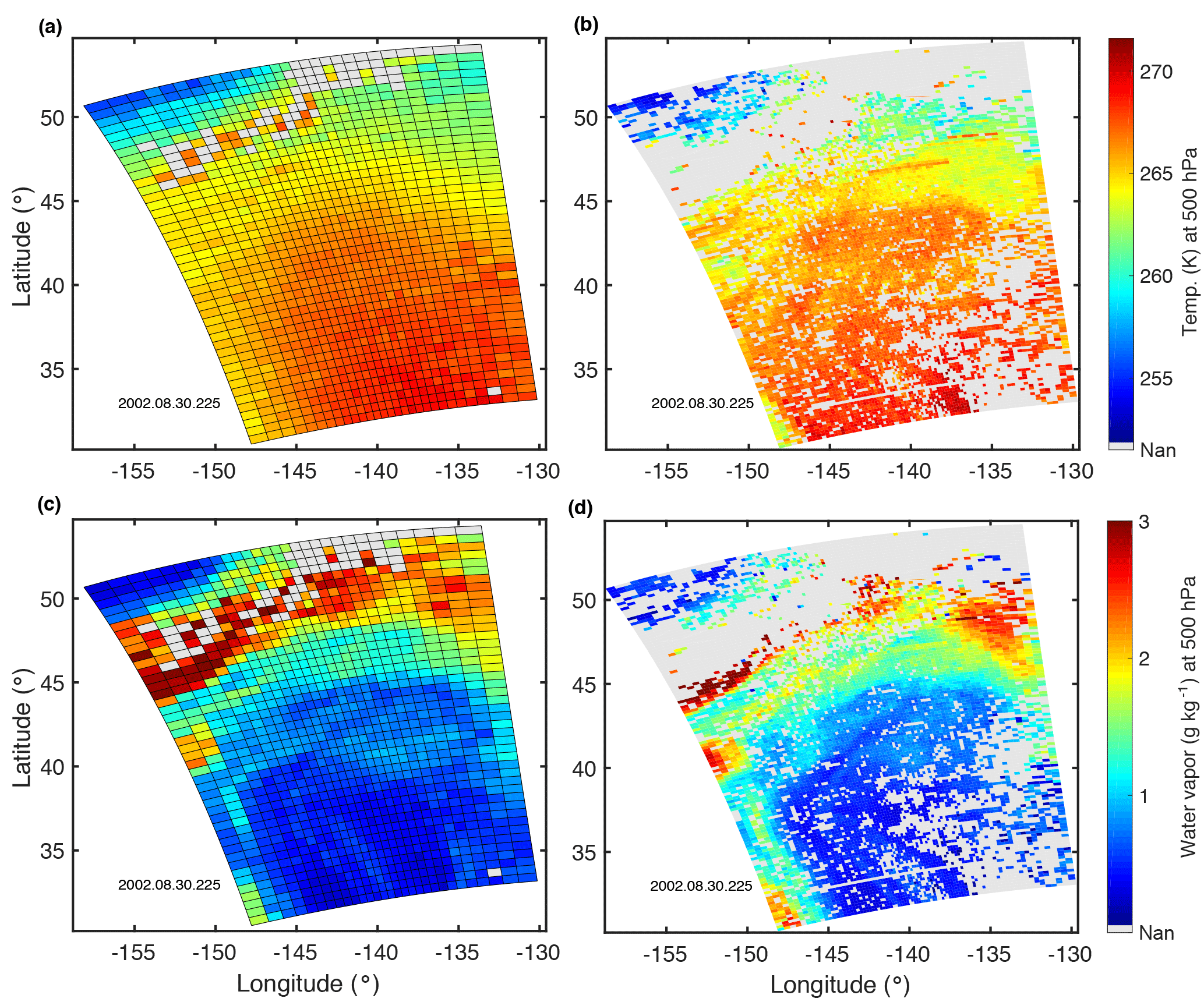
Figure 1(a) Example of an AIRS–AMSU–HSBv6 temperature field at 500 hPa in a granule above the North Pacific Ocean – derived from soundings made during an ascending part of Aqua's orbit, (b) the temperature field using AIRS–OE retrievals, and (c, d) the corresponding moisture fields (the water vapor mass mixing ratio). Gray shading indicates that there was no acceptable retrieval.
Kahn and Teixeira (2009) (KT09 hereafter) used satellite observations of temperature (T) and the specific humidity of water vapor (q) to derive sensitivities of scaling exponents to multiple factors such as the location on Earth (e.g., land, ocean, latitude), the season, and the existence of clouds or clear sky. The underlying causes of these variations and more complex phenomena, such as scale breaks and reverse scale breaks (demonstrated to exist by KT09), are not yet fully understood. One of the reasons may be the paucity of extensive observational data sets that correspond to well-defined atmospheric conditions over several orders of length scales. Clear patterns of scaling exponents only appear after averaging over a sufficient time period on the order of a season (KT09).
A myriad of investigations using atmospheric variability generated by numerical models have been performed. Jonker et al. (1999) used a large-eddy simulation (LES) model to show that passive scalars in a turbulent field exhibit different power spectra than the thermodynamic variables themselves. Cusack et al. (1999) used the horizontal variance of moisture with global weather model analysis data and constructed a cloud parameterization from it. Hamilton et al. (2008) showed a transition from a steep k−3 law to a shallower law in the kinetic energy spectrum of a general circulation model (GCM).

Figure 2(a) Illustration of a water vapor mass mixing ratio field at 500 hPa using AIRS–OE retrievals that are inside a 15.4∘-diameter circle and (b) inside two 6∘-diameter circles. A dark gray shaded pixel inside a circle indicates that there was no acceptable water vapor content estimate. The granule, which is in an ascending part of Aqua's track above the South Pacific Ocean, has a relatively large yield (83 %). However, it is apparent that atmospheric clouds are inhibiting retrievals around (156∘ W–13∘ S).
As with observations, numerical simulations have their own limitations considering the range of scales that are represented. Due to computational restrictions, LES models are not able to accurately simulate synoptic systems. GCMs and cloud resolving models (CRMs) are not able to accurately resolve smaller-scale processes (e.g., turbulence, shallow convection) that affect variance scaling exponents at all scales. Parameterizations of unresolved processes are based on assumptions about variance scaling exponents derived from larger scales (Bogenschutz and Krueger, 2013; Tompkins, 2002; Teixeira and Hogan, 2002; Larson et al., 2002), and therefore, cannot be used to infer independent estimates of variance scaling exponents near the subgrid-scales. In short, there remains a need for numerical and observational investigations that report the statistics of scaling exponents over a larger range of length scales, in particular near the GCM subgrid-scale (Kahn et al., 2011). A review of scaling properties in numerical models is found in Lovejoy and Schertzer (2013).
In a follow-up to the methodology described by KT09, this work presents a new variance scaling method that is applied to vertically resolved, satellite derived T and q with higher horizontal resolution than previously reported. The new variance scaling method enables the calculation of instantaneous variance scaling exponents along the swath of Earth observing satellites. For a particular horizontal two-dimensional atmospheric field (e.g., T or q) at a particular pressure level or altitude in the atmosphere, the standard deviations are calculated over spatial areas for a range of length scales from which variance scaling exponents are derived. Areas are chosen to be of circular shape and are placed along the track of a satellite. Variance spectra are estimated by varying the diameter of the circular areas. Then exponents are derived by fitting power law exponents to the data. To obtain robust estimates, a Monte Carlo method is employed that randomly places smaller circles within the largest diameter circle.
The paper is organized as follows. Section 2 describes the temperature and specific humidity datasets, which is followed by the introduction of the new variance scaling method (Sect. 3). The variance scaling results are presented in Sect. 4. Lastly, Sect. 5 discusses the implications and conclusions of the main findings, and suggests future research that is enabled with this novel approach.
The T and q profiles are derived from high-spectral-resolution infrared (IR) observations made by the Atmospheric Infrared Sounder (AIRS) (Aumann et al., 2003; Chahine et al., 2006) onboard the Aqua spacecraft (Parkinson, 2003). The Aqua satellite is one of the Earth Observing System (EOS) satellites and shares its near-polar (98∘ inclination) orbit with other satellites that form the afternoon A-Train constellation (Stephens et al., 2008). Aqua orbits the Earth at ∼ 705 km altitude in a sun-synchronous orbit with an equatorial crossing of 13:30 (01:30) local time for ascending (descending) orbital segments. With a swath width of 1650 km, the AIRS instrument is able to provide a near-global daily coverage.
2.1 Three types of AIRS standard retrievals
The AIRS instrument is a cross-track scanning spectrometer with 90 AIRS–IR ground footprints per swath and results in a horizontal resolution of 13.5 km at nadir view. The self-calibrating instrument enables the estimation of vertical profiles of several atmospheric variables (e.g., temperature, humidity) and minor gases (e.g., ozone, carbon dioxide) from the surface up to an altitude of 40 km with a quality approaching conventional radiosonde soundings and a vertical resolution of one kilometer (Chahine et al., 2006). The T and q bias and root-mean-square estimates based on radiosonde matchups generally affirm pre-launch requirements of AIRS soundings (Divakarla et al., 2006; Wong et al., 2015).
AIRS is accompanied by two synchronized and aligned microwave instruments. The Advanced Microwave Sounding Unit (AMSU) is a two-unit microwave radiometer with 15 channels that observe frequencies between 23 and 89 GHz including the 60 GHz oxygen band, and a horizontal resolution of 45 km at nadir view. The Humidity Sounder for Brazil (HSB) is a four channel radiometer that observes frequencies between 150 and 190 GHz, centering on the 183 GHz water vapor line, and has a horizontal resolution of 13.5 km at nadir (Lambrigtsen and Calheiros, 2003).

Figure 3The standard deviation of the temperature at 500 hPa as a function of length scale l using AIRS–IR (magenta open circles), AIRS–AMSU (blue open circles), AIRS–AMSU–HSB (green open circles) and AIRS–OE (red open circles) on double logarithmic axes with the slope (black solid line) and the slope (black dotted line) in a circular area with a diameter of 15.4∘ located over (a) the North Pacific Ocean (b) Russia (c) Ethiopia and (d) the South Atlantic Ocean.
The microwave instruments are used together with IR spectra by applying a process called cloud clearing (Susskind et al., 2003). During the process, the horizontal resolution is coarsened from 13.5 to 45 km because all of the variability in the AMSU footprint that contains nine co-aligned AIRS footprints is assumed to arise from cloud variations. The cloud-cleared spectra are then used to retrieve T and q profiles for three different instrument combinations: AIRS–AMSU–HSB, AIRS–AMSU, and AIRS–IR (also termed AIRS-only), the last of which does not use microwave channels but is still obtained at the same spatial resolution as AIRS–AMSU and AIRS–AMSU–HSB (Chahine et al., 2006).
The three-instrument AIRS suite enables the estimation of three-dimensional (3-D) atmospheric profiles along the orbit of Aqua, since 30 August 2002 until present (except until 5 February 2003 for HSB). Swath measurements are organized in files that contain six minutes of data (Level 2) and are termed a “granule”. Each day 240 granules are produced, each consisting of 30 × 45 vertical profiles of T and q. Figure 1a displays an AIRS–AMSU–HSB Version 6 (v6) temperature field at 500 hPa in the very first granule that is available at NASA Goddard Earth Sciences (GES) Data and Information Services Center (DISC). Further detail about the AIRSv6 datasets are found in Susskind et al. (2014).
2.2 AIRS infrared-only optimal estimation (AIRS–OE)
Other alternative methods are undergoing development that treat clouds during the retrieval process through a more sophisticated approach without reducing the horizontal resolution of the T and q fields that are described in Chahine et al. (2006). The optimal estimation (OE) retrieval system for AIRS (AIRS–OE) is described by Irion et al. (2018) and is used in addition to the three coarser-resolution AIRS data products described previously. The methodology is based on the works of Bowman et al. (2006) and Rodgers (2000). Cloud detection and cloud property estimation is enhanced with coincident high spatial resolution imaging data from the Moderate Resolution Imaging Spectroradiometer (MODIS) instrument with a horizontal resolution of 0.25–1.0 km at nadir and a swath width of 2330 km and also resides on EOS Aqua with AIRS (King et al., 2003; Parkinson, 2003; Platnick et al., 2003).

Our approach is to calculate standard deviations as a function of length scale, then scaling exponents are calculated that correspond to a particular range in length scales (as in KT09). The scaling exponents obtained using standard deviations are referred to as “variance scaling” exponents.
If a power-law relation exists between the standard deviation and the length scale, then given two length scales l1<l2 with standard deviations σ1 and σ2, the scaling exponent α is as follows:
When plotting the standard deviation as a function of length scale, while using logarithmically scaled horizontal and vertical axes, the scaling exponent α determines the slope of the line from (l1,σ1) and (l2,σ2). This line is straight if a power-law relation exists and is half as steep as for variances, which can equivalently be used instead of standard deviations to calculate the variance scaling exponents (Vogelzang et al., 2015).
Following KT09, αL is defined as the “large-scale” exponent for scales between 6 and 12∘, and αS is defined as the “small-scale” exponent for scales between 1.5 and 4∘. In addition, we added a third exponent αT that is defined as the “tiny-scale” exponent for scales between 0.5 and 1.5∘. The length scale is expressed in degrees over great circles. To relate the computed α values to the more commonly used power spectral exponents β, α values are interchanged with β values by using the following equation (KT09, Davis et al., 1996; Yu et al., 2017):
The well-known and correspond to and α=1, respectively. Below we describe the estimation of standard deviations within the AIRS swath following the ground track of Aqua.
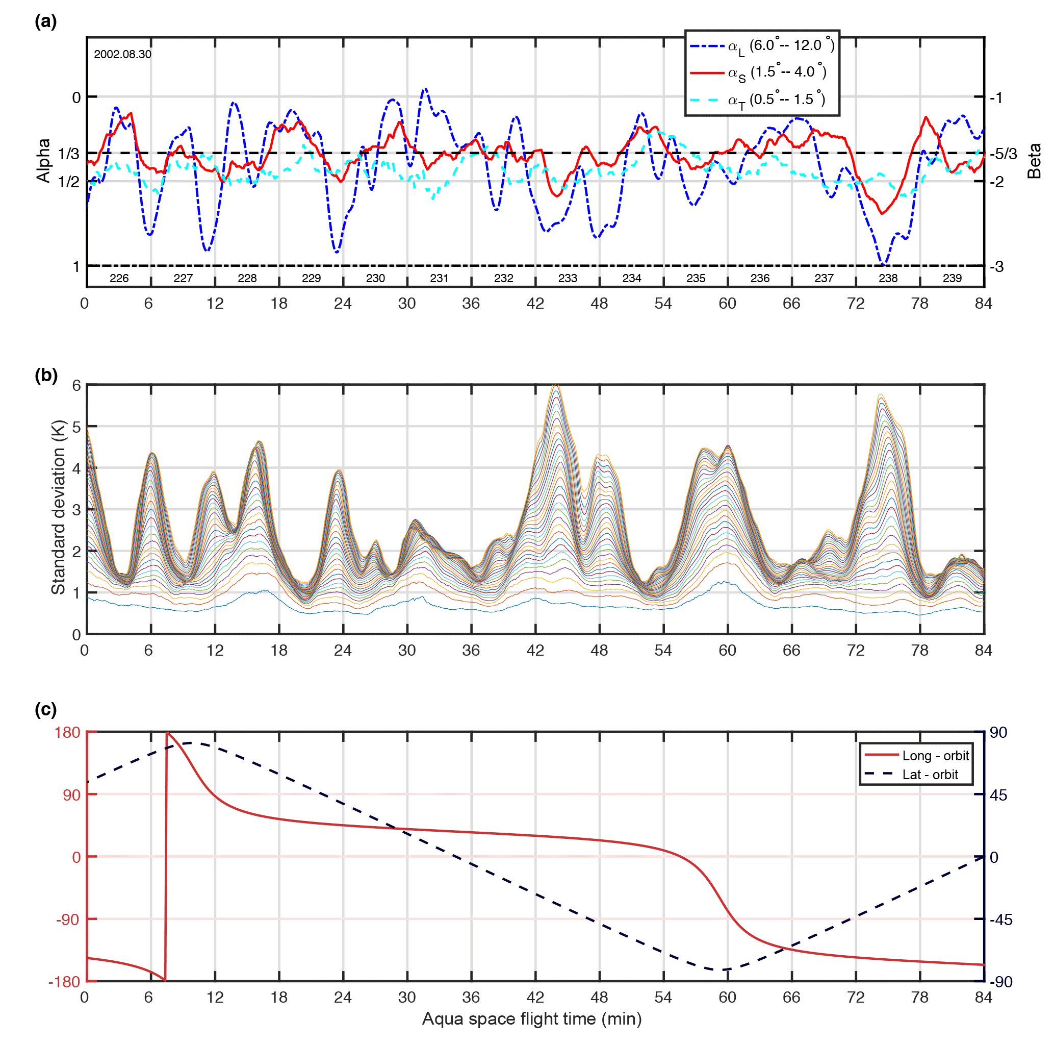
Figure 5(a) AIRS–OE temperature 500 hPa variance scaling exponents αL, αS and αT as a function of Aqua's flight time. The right axis displays the β value. (b) The standard deviations using length scales (lowest line) up to (usually the highest line) and (c) Aqua's longitude (left axis) and latitude (right axis).
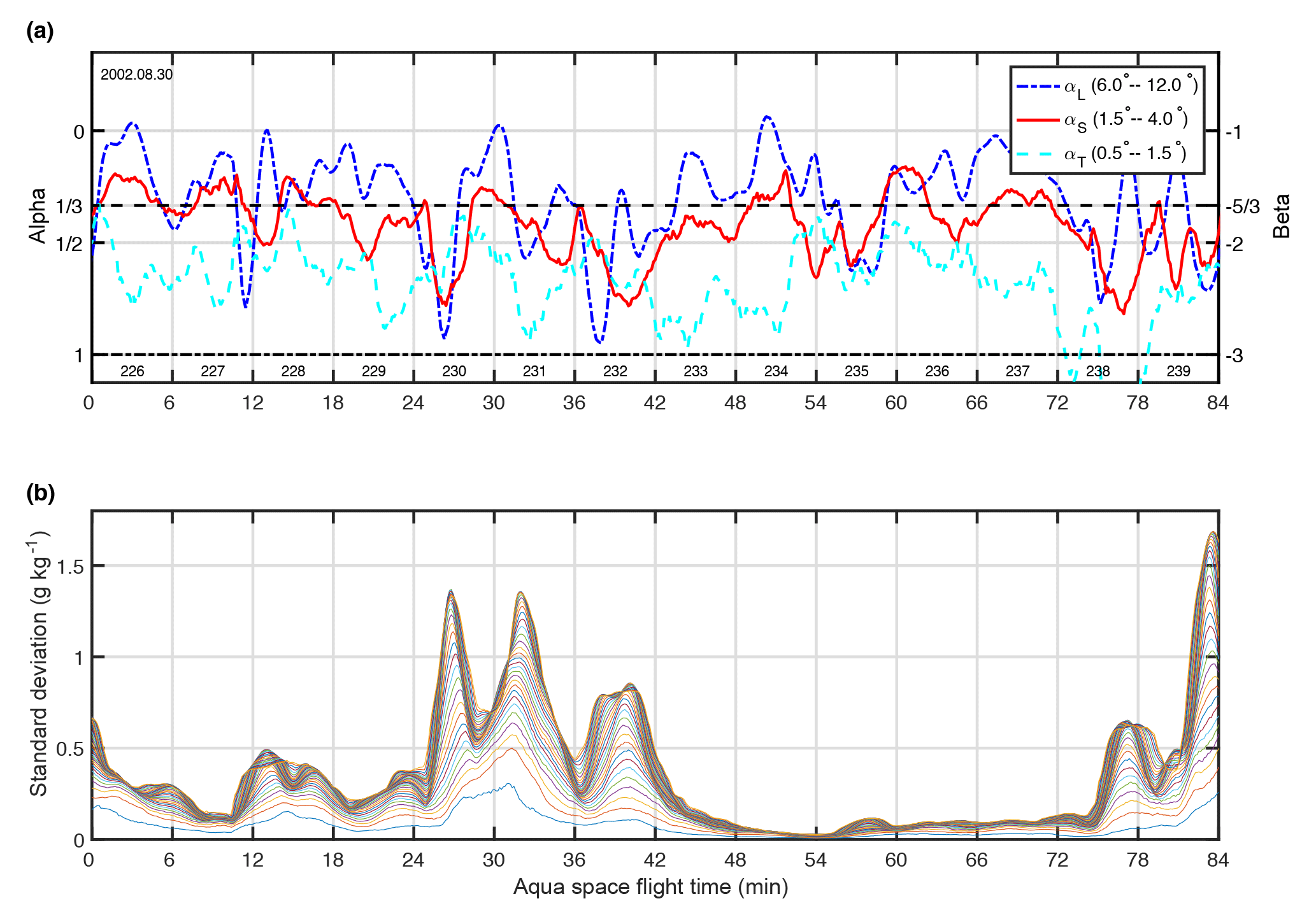
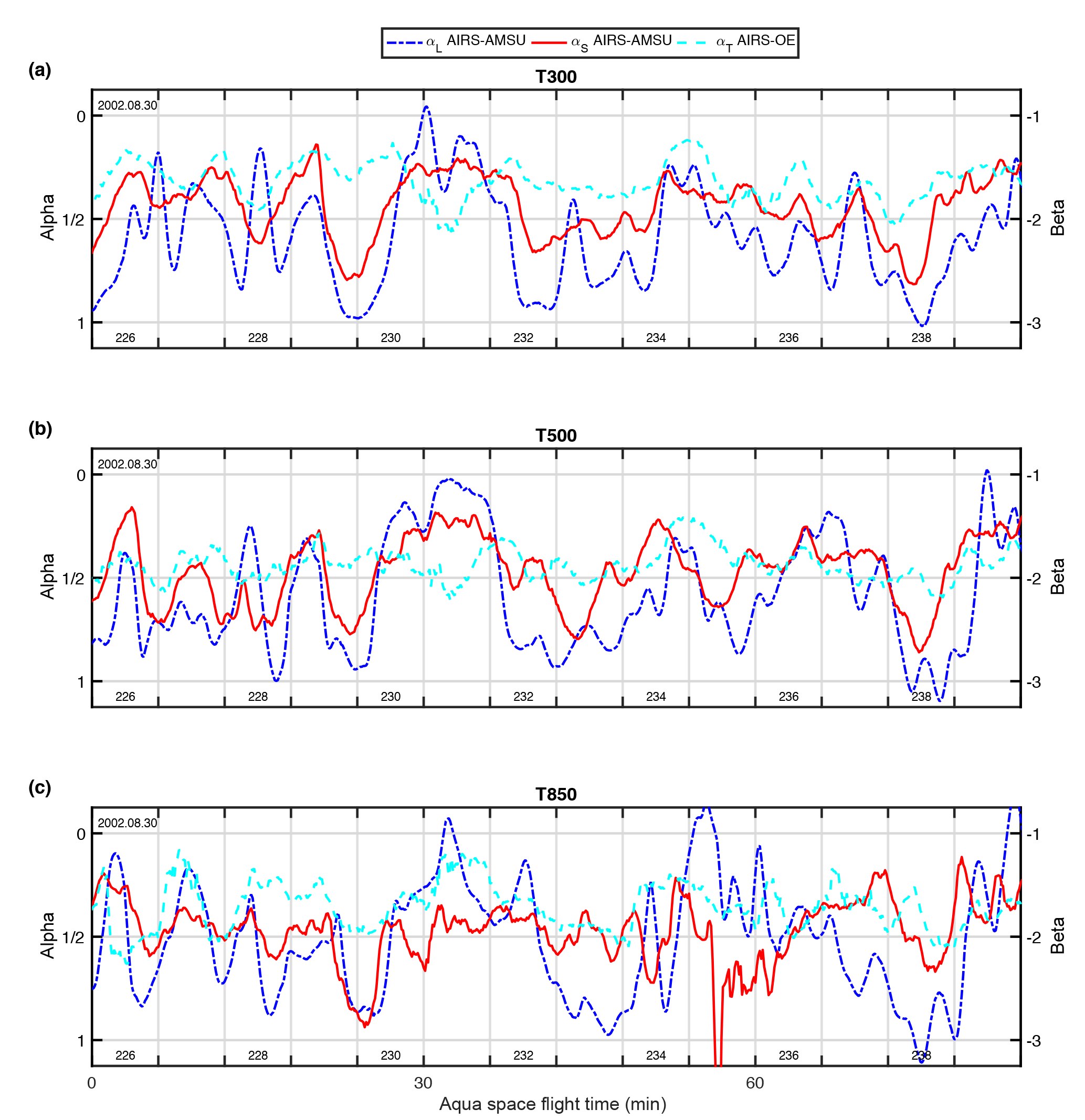
Figure 7Variance scaling exponents αL (blue lines), αS (red lines), and αT (cyan lines) as a function of Aqua's flight time for temperature (a) at 300 hPa, (b) at 500 hPa, and (c) at 850 hPa using AIRS–AMSU (αL and αS) and AIRS–OE (αT). Additionally, the date (left upper corner) and granule numbers (bottom) of the corresponding β values can be seen on the right axis.
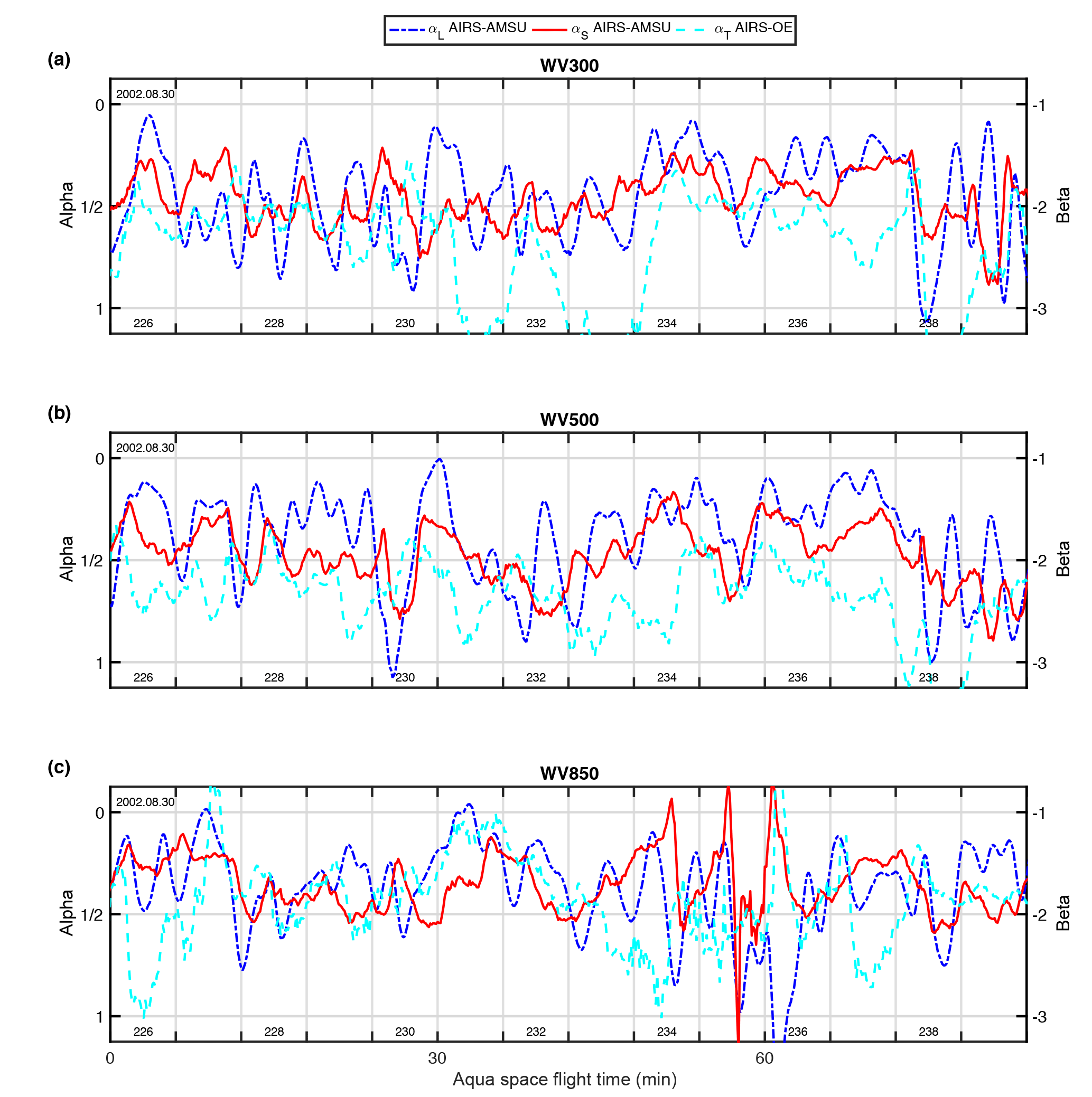
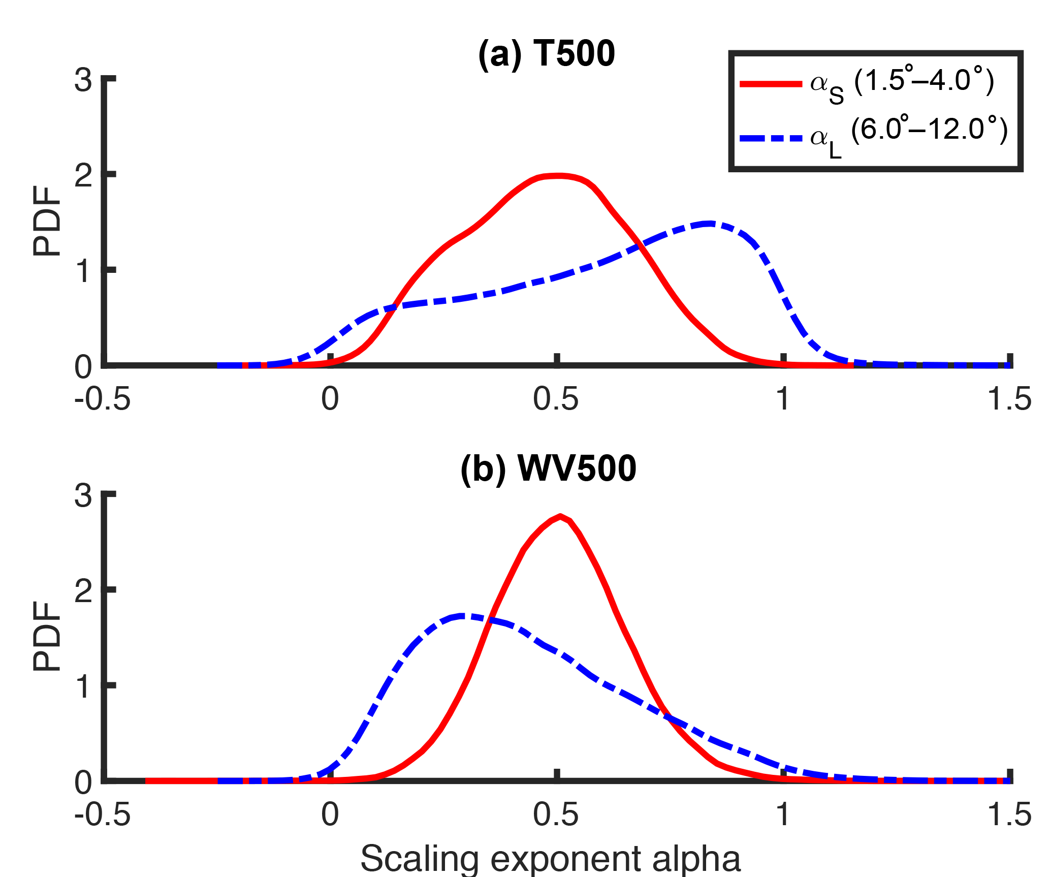
Figure 9Probability density functions of AIRS–AMSUv6 (a) temperature 500 hPa and (b) water vapor 500 hPa, scaling exponents αL (6.0–12∘) and αS (1.5–4.0∘) derived from five days of observations.
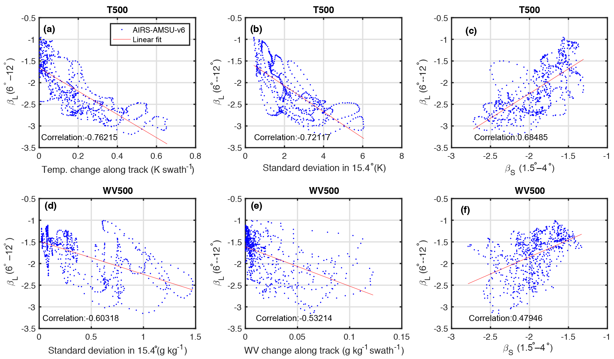
Figure 10Scatterplots, linear fits, and correlations between physical quantities and the slope βL derived using AIRS–AMSU temperatures at 500 hPa (T500) or water vapor at 500 hPa (WV500) along a 96 min segment of the Aqua track. Panels are ordered from strong (a) to weak (f) absolute correlations.
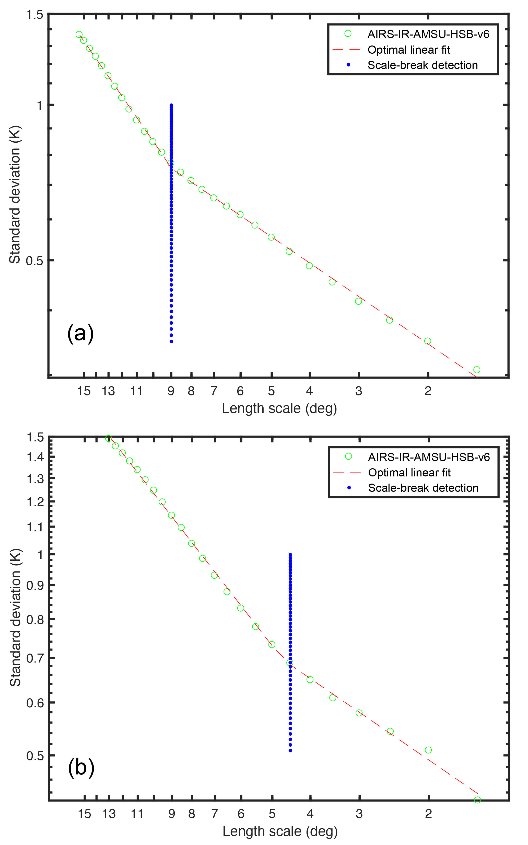
Figure 11Two variance-scaling plots for AIRS–AMSU–HSB derived temperature at 500 hPa with detected scale breaks: (a) North Pacific Ocean (40.3∘ N, 141.5∘ W) (b) North Pacific Ocean (44.6∘ N, 142.9∘ W). In (a) the slope changes at 9∘ and in (b) at 4.5∘.
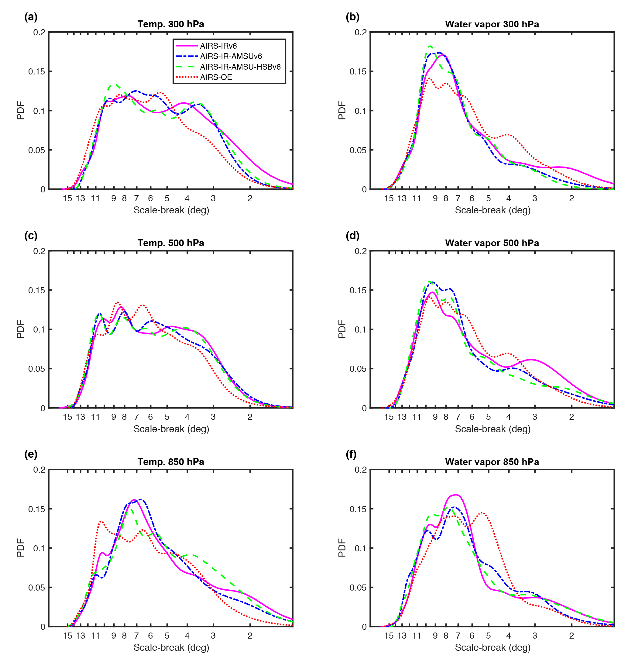
Figure 12Probability density functions of the scale break length scale using (left) temperature and (right) water vapor fields at three pressure levels.
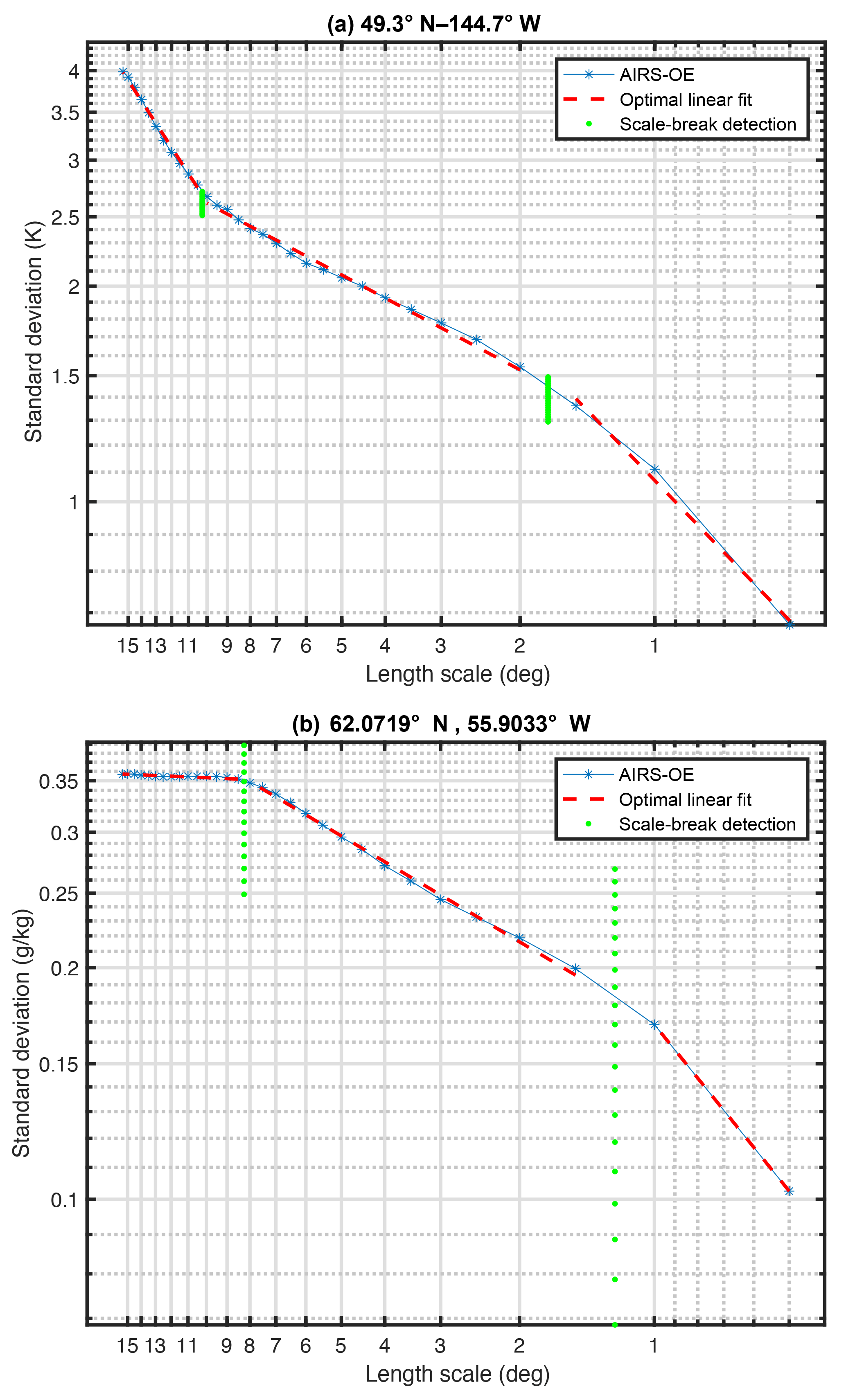
Figure 13In these double scale break examples it can be seen that the slope can change at scales below 1.5∘. The standard deviations are calculated with AIRS–OE derived (a) temperature and (b) water vapor mass mixing ratio at 500 hPa.
3.1 Circular geometry
Standard deviations are computed within circular areas of diameter l. The maximum length scale is determined by the fixed swath width of AIRS, . In that limiting case, a circle with radius 7.7∘ is positioned with its center on Aqua's ground track (at nadir), after which the standard deviation of valid T and q values are calculated within the circle. A depiction of the 500 hPa q using AIRS–OE retrievals that are inside a 15.4∘ diameter circle is found in Fig. 2a. The smallest length scale is the other limiting case and is determined by the horizontal resolution of the observations. Here, we require that the minimum number of valid retrievals that are necessary to calculate a standard deviation from a circle with a given diameter is five, as assumed in KT09. Taking this requirement into consideration for AIRS–OE retrievals, the smallest length scale and hence the smallest diameter of the circles is chosen to be l=0.5∘. For the three coarser-resolution AIRSv6 data products (AIRS–IR, AIRS–AMSU, AIRS–AMSU–HSB) the smallest length scale is chosen to be l=1.5∘.
3.2 Monte Carlo calculations
To obtain standard deviations corresponding to length scales smaller than (i.e., ), smaller circles are randomly placed inside the largest circle. Given that a smaller circle with diameter is randomly placed within the largest circle, we further require that the smallest circle is entirely within the larger circle. Then, the standard deviation of T and q values located within the smaller circle are computed.
To obtain a more robust estimate, a Monte Carlo estimation procedure is employed. The random placement is repeated 10 000 times for each of the smaller circle diameters. The average standard deviation over all 10 000 values is used as the estimate of the standard deviation corresponding to l. The random placement should be done such that the 10 000 smaller circles cover the largest circle as uniformly as possible. This procedure is repeated for all length scales for AIRS–OE and down to 1.5∘ for AIRSv6 products. Two out of the 10 000 smaller circles at are displayed in Fig. 2b.
3.3 Along-track instantaneous variance scaling estimates
The intent of this method is to move the 15.4∘ diameter circle along with the orbit of the Aqua satellite to estimate standard deviations and therefore variance scaling exponents at each successive scan line along the satellite ground track. This requires stitching together successive granules. Therefore, a novelty of this approach is that the variance scaling can be derived instantaneously (i.e., no time averaging as in KT09).
The diameters of the circles can vary with arbitrary increments; we select 0.5∘, which should yield sufficient resolution to resolve scale-dependent breaks and other behavior introduced in Sect. 4. After the standard deviations are calculated as a function of length scale, the three exponents (i.e., the slopes) are estimated by a least squares fit (Weisstein, 2017).
For αL, the formula of Weisstein (2017) is:
where xi=li and yi=σi, with and n=13. For αS and αT, the formulas are used with , , and n=6 and n=3, respectively.
We note that βL, βS, and βT are the analogs of αL, αS and αT and will be interchangeably used with α values as β values are more commonly used in the literature.
3.4 Scale break detection
To quantify the length scale lb at which the exponents change (e.g., from to ) the standard deviation as a function of l is approximated by two power laws, which is equivalent to fitting two straight lines in a double-log scaled figure. When using the higher spatial resolution AIRS–OE retrieval, the double scale break is examined by fitting three straight lines in the variance scaling plots. To do this optimally, we iterate over all possible (double) scale break positions to find the two (three) fitted lines that minimize the sum of the squares of the vertical offsets from the data to the lines. Since such a minimum always exists, albeit at times very subtly, we find an optimal single scale break l in each variance scaling diagram for AIRS–AMSU–HSB, AIRS–AMSU, and AIRS–IR, and two scale break values of l for AIRS–OE. In future work, thresholds could be used to make a distinction between variance scaling diagrams with and without scale breaks.
4.1 Variance scaling diagrams
To demonstrate the methodology, we aim to construct variance scaling diagrams that are analogous to Fig. 3 of Nastrom and Gage (1985). In this work, Fig. 3 shows the standard deviations of 500 hPa T at four selected locations on the Aqua track. The four locations are shown because they encompass typical behavior of the scaling. We note that the scaling behavior drastically changes at these locations depending on the day. The four available AIRS retrievals are shown in order to gain insight regarding the uncertainty of the scaling that arises from sampling, retrieval algorithm, and observation frequency differences.
The standard deviation typically increases as a function of l; only in Fig. 3c do we find that the standard deviation decreases at larger l for AIRS–OE. In Fig. 3a this increase is not constant: at larger l, , while at smaller l, for AIRS–OE. In Fig. 3a, the slope changes between and and is a clear example of a well-behaved scale break. Observe in Fig. 3c that the slope at smaller l is steeper than at larger l, and is an example of a reverse scale break previously reported in KT09 for specific humidity. In Fig. 3d, there is no clear scale break at all except for some subtle fluctuations in the spectra.
The differences in the standard deviations among the three coarser-resolution AIRS data products are generally small and are partly attributed to sampling differences from clouds. AIRS–OE generally yields higher standard deviations, most notably in Fig. 3b, which is to be expected because of the higher spatial resolution. Other contributions to discrepancies among the retrievals may be attributed to spatial sampling differences that arise from differences in the spatial distributions of unsuccessful retrievals. Given that the variance of T and q is highly location dependent, the additional sampling provided by the microwave frequencies will also lead to differences in the four retrievals in Fig. 3. Observe that the relative differences between the slopes of the four different retrievals appear to be smaller than the magnitude differences themselves.
The corresponding q spectra at 500 hPa are shown in Fig. 4. The scaling of q in Fig. 4a is similar to scaling in T in Fig. 3a; however, the slopes appear to be closer to at smaller l in Fig. 4a. In Fig. 4b, a reverse scale break is clearly visible near . In Fig. 4c, the discrepancies between the four retrievals are more significant at larger l, where AIRS–OE shows a decreasing standard deviation as a function of increasing l. However, the AIRS–OE with a peak around 8∘ may be a result of finer-scale fluctuations that are only captured by AIRS–OE. At smaller scales, the slopes are similar and reside between and . In Fig. 4d, the slopes are close to at larger l, then are close to (i.e., α=0) around , then again increase (α) and decrease (β) at smaller length scales, in sharp contrast to T in Fig. 3d.
4.2 Along-track variance scaling
We now focus on the scaling exponents αL, αS, and αT, along 84 min of the Aqua track starting at the second granule available in the AIRS archive. We estimate scaling exponents 500 hPa T and q. The 84 min dataset is a very small subset of the ∼ 15 year AIRS dataset and corresponds to just under one complete orbit. The centers of consecutive 15.4∘ diameter circles are 8 s apart from each other, corresponding to the time it takes to make 30 AIRS–AMSU soundings along the width of the swath. As consecutive 15.4∘ circular areas have high overlap, there are large correlations in exponents along neighboring scan lines.
The three scaling exponents derived from AIRS–OE retrievals are shown in Fig. 5a. Observe that the exponent αL fluctuates between 0 and 1 (left vertical axis) that corresponds to β between −1 and −3 (right vertical axis). The exponent αS has smaller fluctuations around (). The exponent αT exhibits even smaller fluctuations than αS and usually resides between 1∕2 and 1∕3, and corresponds to β between −2 and −5/3.
The standard deviation estimates from which these scaling exponents are calculated are shown in Fig. 5b. The lowest line is the standard deviation that corresponds to , the line above corresponds to , and so forth. The standard deviations are usually, but not always, increasing as a function of length scale.
Local maxima of the standard deviation at 15.4∘ co-align with local maxima of αL (local minima of ). A large standard deviation at synoptic scales is indicative of meridional temperature gradients along the satellite track, and correlates well with αL (shown later). The latitude and longitude at nadir are depicted in Fig. 5c.
Increased separation between the three values of α (Fig. 5a) suggest the existence of scale breaks at those latitudes. For example at 75 min (40∘ S), αL=1 (), while αS=0.6 and αT=0.5. Nearer to the equator around 33 min, the estimates are reversed: αL=0, αT=0.5 nearly unchanged, and αS is in between the two other values of α, indicating a double reverse scale break (steeper exponents at smaller scales). Around 58 min near Antarctica, the three values of α are nearly equal with no apparent scale breaks. Analogous variance scaling diagrams would be similar to that shown in Fig. 3.
The corresponding q exponents are shown in Fig. 6a. The αL has a similar range as the T exponent. The αS for q is slightly larger than for T. However, the αT for q is significantly larger than for T. Figure 6b depicts the standard deviations of q. In the tropics (location from Fig. 5c), the standard deviation is much larger than in the extratropics (e.g., compare granules 231 and 235). Maximum values of standard deviation are generally co-aligned with maximum values of αL.
4.3 Variance scaling at 850, 500, and 300 hPa
Previous studies have demonstrated that the magnitude of scaling exponents depends on altitude, surface type, and cloud cover (e.g., KT09). Therefore, we show variance scaling exponents along the same orbit segment at three pressure levels (300, 500, and 850 hPa) in Fig. 7 for T and Fig. 8 for q. The results are typically noisier at lower pressure levels (e.g., compare Fig. 7c to a, b) and is consistent with a reduction in the yield (percentage of successful retrievals).
The three coarser-resolution AIRS products are similar when the yield is high. Therefore, we show only AIRS–AMSU derived exponents in Figs. 7 and 8. The αL (blue dash-dotted line) for T fluctuates between 0 and 1, except for a portion of the 850 hPa pressure level (Fig. 7c) around the South Pole (granule 235) where the yield is exceptionally low. The small-scale exponent αS (red solid line) fluctuates within a smaller range except for a portion of 850 hPa around 24 min in which αS=1.
A reverse scale break in the tropics (granule 231) is clearly visible at 500 hPa and to a lesser extent at 850 and 300 hPa, which is consistent with KT09. The scaling exponent αT (cyan dashed line) derived from AIRS–OE fluctuates between αT=0.2 to 0.6 for all time segments at the three pressure levels. Variations with surface type and cloud fraction (not shown) are less obvious in Figs. 7 and 8 and become clearer only after averaging over long time series (e.g., KT09).
The values of α for q exhibit more rapid along-track fluctuations compared to T at the three pressure levels. The αL for q fluctuates between 0 and 1 in Fig. 8. The αS for q is similar to T, but αT for q is typically larger than 0.5 () and has a larger dynamic range for q than for T (compare Figs. 7 and 8). In granule 233 at 300 hPa, αT exceeds 1.0 ().
4.4 Distributions of variance scaling exponents
Histograms of αL and αS for 500 hPa T and q obtained from five days of Aqua orbits are shown in Fig. 9. To increase the computational speed, only 100 circles are used in the Monte Carlo method described earlier, which leads to a slight increase in the number of extreme values of αL and αS. The histograms of αL have larger ranges than αS, both for T and q. The αS exhibit a more symmetric distribution and the maximum number of values is near αS=0.5.
The asymmetry of αL for T is caused by different values in the extratropics and tropics. In the tropics, αL is closer to 0, while in the extratropics it is closer to 1. The values of αS do not have a strong latitude dependency and thus the distribution is more symmetric. The αL for q is skewed in the opposite direction compared to αL for T, because αL is closer to 1 in the tropics and closer to 0 in the exratropics.
These types of statistical distributions are valuable for the development and evaluation of cloud parameterizations based on PDF schemes. This is especially true for αT (not shown); the AIRS–OE retrieval methodology is in development and the sample size from the limited set of granules is unable to yield a robust histogram. Our intent is to instead demonstrate the new scaling approach. A much larger and statistically robust dataset is outside the scope of this work. Furthermore, the computational expense is excessive using the Monte Carlo methodology with 10 000 circles rather than 100, and new ways of improving the speed of the calculations remains necessary.
4.5 Correlation of scaling exponents to other quantities
To relate βL and βS to additional geophysical quantities, correlation analysis is performed using the AIRS–AMSU retrieval and the results are summarized in Fig. 10. A total number of 686 values (the number of L2 retrieval swaths) cover a slightly longer extent of the orbital segment than the 84 min portion used in Sect. 4.2 and 4.3. The largest correlation coefficient (r) is found between βL and the mean T gradient (slope) in the along-track direction of Aqua at nadir view (Fig. 10a). The T change we consider is the difference between the average 500 hPa T over consecutive 15.4∘ diameter circles. If the T gradient is large, βL is closer to −3. If the T gradient is small or near zero, βL is closer to −1.
The βL also correlates strongly with the standard deviation of T in the 15.4∘ diameter circle (Fig. 10b); this confirms the co-alignment of peaks observed in Fig. 5a and b. For q, βL is moderately correlated with the standard deviation in the 15.4∘ diameter circle (Fig. 10d) and the along-track q gradient (Fig. 10e). The exponents βL and βS are positively correlated for both T (Fig. 10c) and q (Fig. 10f), but the correlations are notably larger for T. The surface type (land vs. ocean) is not strongly correlated with βL or βS at 850 hPa (not shown). Lastly, the cloud fraction has a rather weak correlation with βL and βS at 500 hPa (not shown); again, a larger sample size may yield different results.
4.6 Scale break detection results
Figure 11 shows an example of the methodology to detect scale breaks. This example makes it clear that the length scale of scale breaks lb varies substantially along the Aqua tracks. The lb differ by a factor of two (9 and 4.5∘, respectively). lb fluctuates by an order of magnitude between 1.5 and 15∘ along the Aqua track at 850, 500, and 300 hPa for all four AIRS retrieval products, and for both T and q.
We show PDFs in Fig. 12 to gain additional insight in the distributions of lb. The resolution of AIRS–OE is fixed to such that similar scale breaks will be detected as the three standard AIRS data retrievals. The maximum frequency of occurrence in the PDFs is between 7 and 10.5∘ for T and between 5 and 8∘ for q at 850 hPa (Fig. 12e, f), between 8 and 11∘ for T at 500 hPa (Fig. 12c) and around 9∘ for q at 500 hPa (Fig. 12d), between 5.5 and 9∘ for T at 300 hPa (Fig. 12a) and around 9∘ for q at 300 hPa (Fig. 12b). These results, to some extent, are in agreement with the 500–700 and 450–750 km lb reported by Gage and Nastrom (1985) and Tung and Orlando (2003), respectively. The PDFs of T (Fig. 12a, c) have less well-defined maxima compared to q (Fig. 12b, d, f), except for T at 850 hPa (Fig. 12e), in which a clear peak is apparent at 7∘ (Fig. 12e) for three AIRS standard retrieval products. A tentative physical and algorithmic explanation for the large spread of lb is provided in Sect. 5.
Lastly, an example of a double scale break detection is applied to the AIRS–OE dataset for T and q in Fig. 13. This example once again demonstrates the variety of variance scaling that is potentially observable in the atmosphere. The slope in the spectrum is steeper at the smaller scales less than 1.5∘. This behavior is of importance for cloud parameterizations based on PDF schemes. Less variance exists at the smaller scales than what one obtains from a simple extrapolation of exponents at larger scales to smaller scales; this was previously shown with in situ aircraft observations in Kahn et al. (2011) in a limited region of the subtropical southeastern Pacific Ocean.
The scale-dependent variability of temperature (T) and specific humidity (q) is derived from Level 2 satellite swath data. The variance scaling of T and q uses data from the Atmospheric Infrared Sounder (AIRS; Chahine et al., 2006) instrument suite onboard the Aqua satellite. While these exponents are frequently close to the canonical and values, deviations from these values are more the rule than the exception. The large scale exponents βL that correspond to length scales between 6 and 12∘ fluctuate between −3 and −1, respectively.
The precise value of βL depends strongly on the standard deviation of T and q within larger spatial areas. The synoptic-scale T and q gradient in the along-track direction also impacts the magnitude of βL. When the large scale fluctuations or gradient are large, then . When large scale T fluctuations are reduced such as in the tropics, and the atmosphere is dominated by small scale fluctuations, . In the tropics, small-scale T fluctuations dominate because of the preponderance of deep convection. In contrast, large-scale q fluctuations are more dominant in proximity to and within the tropics, which results in .
The small-scale variance scaling exponents βS that correspond to length scales between 1.5 to 4∘ are more often near to −2, and less often close to −3. By using recently developed retrievals from single-footprint AIRS data (Irion et al., 2018), we show that at the smaller scales from 0.5 to 1.5∘, the exponents βT are closer to −2 for T and slightly lower (between −2 and −3) for q. The PDFs of small-scale βS exhibit a maximum around −2 for both T and q. This is somewhat surprising since previous studies have suggested values closer to .
Deviations from typical values of β ( and −3) have been reported in the literature previously (e.g., KT09). Lovejoy et al. (2008) show that exponents derived from drop sondes over the northern Pacific Ocean reside in between and −3 and have strong height dependence. It was also shown that the vertical exponents are not equal to the horizontal exponents, and suggests 3-D anisotropy. Lovejoy et al. (2009) and Pinel et al. (2012) showed that scale breaks detected by in situ aircraft observations may be the result of 3-D anisotropy in atmospheric properties. In Pinel et al. (2012), scale breaks are observed in the 100–500 km range with horizontal exponents that transition from to −2.4. In the vertical direction, an exponent of −2.4 is derived and suggests that gently sloping isobaric aircraft trajectories are the source of the transition to −2.4. Since the T and q exponents reside on isobaric surfaces (e.g., 500 hPa) in this work, one may expect that the vertical exponents may alias into the large-scale horizontal exponents. However, we do not find a clear indication of , although a focused effort on obtaining vertical scaling exponents with satellite soundings warrants further investigation. Unfortunately, the relative coarse vertical resolution of ∼2 km from AIRS retrievals is not ideal for obtaining reliable estimates of vertical scaling exponents; dropsondes and radiosondes remain the standard and are much better suited to this observational challenge.
The methodology described uses circles to calculate standard deviations. The optimal shape of an area used to calculate variance remains an open question. Rectangles have been used previously (e.g., KT09) and are generally accepted, because GCM grid columns are often (nearly) rectangular. The orientation of a rectangle or square should not be of major importance when calculating variance scaling exponents. One could argue that incremental rotation of the rectangle about a central axis could be used to trace out the area of a circle. Within each rectangle, the variance can be calculated, and the same for each slight rotation of the rectangle about the center axis, until it is rotated 360∘. This procedure of incremental rotation could be performed with any arbitrary shape. In all cases, the circle is the final result, and therefore one may conclude that the circle is the “optimal shape” to calculate variance scaling exponents. A circle is optimal in the event that rotational symmetry is desired if, for example, the underlying field is isotropic. This is consistent with Pressel and Collins (2012) who found that variance scaling of q is approximately isotropic.
A major advantage of the “poor man's spectral analysis” method (Lorenz, 1979) is that relatively small datasets are sufficient to estimate variance scaling exponents. Reliable spectral power diagrams of observational data arise only after averaging over relatively large datasets. For instance, Nastrom and Gage (1985) obtained their spectral power diagrams by averaging over observations collected during 6000 commercial aircraft flights. The calculation of spatial variances is still possible in the event of missing or poor quality data, in which case conventional spectral analysis cannot be employed (Vogelzang et al., 2015).
The variance scaling exponents are computed nearly instantaneously without using multiple satellite overpasses (no time averaging) in this work. The exponents are derived from satellite observations within a 15.4∘ diameter circle over a few minute time window, thus strictly speaking, the method is “approximately” instantaneous. A result of the instantaneous approach is that a much wider variety of scaling exponents is revealed. The large variety of exponents is likely due to some extent from the turbulent structure of T and q fields with long-tailed non-Gaussian distributions (Tuck, 2010). These behaviors may inhibit the precise estimation of variance scaling exponents from observations. Further research is necessary to determine the impacts of the non-Gaussian distribution shapes of T and q on derived exponents, and their scale-dependence of non-Gaussianity. This effect likely contributes to spreading out the PDFs of exponents.
The results show that there is a preference for scale break length scales (lb) around 7∘ (at 850 hPa) and 9∘ (at 500 hPa and 300 hPa). This is slightly larger than the 500–700 and 450–750 km lb reported by Gage and Nastrom (1985) and Tung and Orlando (2003), respectively, and smaller than 1000 km reported by Bacmeister et al. (1996). Pinel et al. (2012) report lb between 100 and 500 km. The spread around these values is large in our results and a preferred length scale is only inferred from the maxima in the PDFs. An explanation for the large spread in the PDFs is that convective systems of different sizes exist. The existence of a reverse scale break depends on the scale of convective systems: the larger the scale, the larger lb. Furthermore, as lb is obtained in the along-track dimension, for instance when the satellite observation transitions from a regime with to a regime with , then the intermediate length scales between 2 and 15∘ are also retrieved in between the two regimes as the circular area advances along the swath. Due to the overlapping nature of the circular areas, this additionally smooths out the peaks in the PDFs, but further work is necessary to quantify the magnitude of this effect compared to the spreading due to non-Gaussianity.
The exponent βT (0.5 to 1.5∘) for q was shown to attain smaller values, i.e., closer to than the exponent βS (1.5 to 4∘). This means that less variance is present at length scales between 0.5 and 1.5∘ than if extrapolated from exponents derived from length scales between 1.5 and 4∘. Scale breaks at subgrid scales in GCMs are of significance for cloud parameterizations in GCMs that extrapolate variability (Tompkins, 2002; Teixeira and Hogan, 2002; Teixeira and Reynolds, 2008).
This novel instantaneous variance scaling methodology may enable detailed examination of the variance scaling of the time evolution of storm systems, such as extratropical cyclones at different stages in their life cycle as previously demonstrated with numerical simulations by Waite and Snyder (2013), or with deep convection along the Mei-Yu front by Peng et al. (2014). The changes in the kinetic energy spectra in Waite and Snyder (2013) and Peng et al. (2014) occur on time scales of hours to several days. We postulate that scaling exponents derived from instantaneous snapshots obtained from satellite swath data will be useful observational constraints for time-dependent spectra generated from numerical modeling experiments. To conclude, it is well known that the time scale of predictability is closely linked to the spatial scale of the phenomenon of interest (Lorenz, 1969). In the case of moist baroclinic waves, steeper (shallower) spectral slopes at small scales for individual baroclinic waves are inherently more (less) predictable as the slope portrays the relative importance of convection within any given disturbance (Zhang et al., 2007). As a result, the instantaneous scaling exponents are expected to potentially offer a new type of observational constraint with relevance to the predictability of individual tropical or extratropical disturbances.
The AIRS version 6 data sets were processed by and obtained from the Goddard Earth Services Data and Information Services Center (http://daac.gsfc.nasa.gov/; Teixeira, 2013). All rights reserved. Government sponsorship acknowledged.
The authors declare that they have no conflict of interest.
Part of this research was carried out at the Jet Propulsion Laboratory (JPL), California Institute of Technology, under a
contract with the National Aeronautics and Space Administration. All authors were partially supported by the AIRS project at JPL.
Edited by: Andrew Sayer
Reviewed by: two anonymous referees
Aumann, H. H., Chahine, M. T., Gautier, C., Goldberg, M. D., Kalnay, E., McMillin, L. M., Revercomb, H., Rosenkranz, P. W., Smith, W. L., Staelin, D. H., Strow, L. L., and Susskind, J.: AIRS/AMSU/HSB on the Aqua mission: Design, science objectives, data products, and processing systems, IEEE T. Geosci. Remote, 41, 253–264, 2003. a
Bacmeister, J. T., Eckermann, S. D., Newman, P. A., Lait, L., Chan, K. R., Loewenstein, M., Proffitt, M. H., and Gary, B. L.: Stratospheric horizontal wavenumber spectra of winds, potential temperature, and atmospheric tracers observed by high-altitude aircraft, J. Geophys. Res.-Atmos., 101, 9441–9470, 1996. a
Bogenschutz, P. A. and Krueger, S. K.: A simplified pdf parameterization of subgrid-scale clouds and turbulence for cloud-resolving models, J. Adv. Model. Earth Sy., 5, 195–211, 2013. a
Bowman, K. W., Rodgers, C. D., Kulawik, S. S., Worden, J., Sarkissian, E., Osterman, G., Steck, T., Lou, M., Eldering, A., Shephard, M., Worden, H., Lampel, M., Clough, S., Brown, P., Rinsland, C., Gunson, M., and Beer, R.: Tropospheric Emission Spectrometer: Retrieval Method and Error Analysis, IEEE T. Geosci. Remote, 44, 1297–1307, 2006. a
Chahine, M. T., Pagano, T. S., Aumann, H. H., Atlas, R., Barnet, C., Blaisdell, J., Chen, L., Divakarla, M., Fetzer, E. J., Goldberg, M., Gautier, C., Granger, S., Hannon, S., Irion, F. W., Kakar, R., Kalnay, E., Lambrigtsen, B. H., Lee, S.-Y., Le Marshall, J., Mcmillan, W. W., Mcmillin, L., Olsen, E. T., Revercomb, H., Rosenkranz, P., Smith, W. L., Staelin, D., Strow, L. L., Susskind, J., Tobin, D., Wolf, W., and Zhou, L.: AIRS: Improving Weather Forecasting and Providing New Data on Greenhouse Gases, B. Am. Meteorol. Soc, 87, 911–926, 2006. a, b, c, d, e
Charney, J. G.: Geostrophic Turbulence, J. Atmos. Sci., 28, 1087–1095, 1971. a
Cusack, S., Edwards, J., and Kershaw, R.: Estimating the subgrid variance of saturation, and its parametrization for use in a GCM cloud scheme, Q. J. Roy. Meteor. Soc., 125, 3057–3076, 1999. a
Davis, A., Marshak, A., Wiscombe, W., and Cahalan, R.: Scale invariance of liquid water distributions in marine stratocumulus. Part I: Spectral properties and stationarity issues, J. Atmos. Sci., 53, 1538–1558, 1996. a
Divakarla, M. G., Barnet, C. D., Goldberg, M. D., McMillin, L. M., Maddy, E., Wolf, W., Zhou, L., and Liu, X.: Validation of Atmospheric Infrared Sounder temperature and water vapor retrievals with matched radiosonde measurements and forecasts, J. Geophys. Res.-Atmos., 111, D09S15, https://doi.org/10.1029/2005JD006116, 2006. a
Fjørtoft, R.: On the Changes in the Spectral Distribution of Kinetic Energy for Twodimensional, Nondivergent Flow, Tellus, 5, 225–230, 1953. a
Gage, K. and Nastrom, G.: On the spectrum of atmospheric velocity fluctuations seen by MST/ST radar and their interpretation, Radio Sci., 20, 1339–1347, 1985. a, b
Hamilton, K., Takahashi, Y. O., and Ohfuchi, W.: Mesoscale spectrum of atmospheric motions investigated in a very fine resolution global general circulation model, J. Geophys. Res.-Atmos., 113, D18110, https://doi.org/10.1029/2008JD009785, 2008. a
Hunt, J. and Vassilicos, J.: Kolmogorov's contributions to the physical and geometrical understanding of small-scale turbulence and recent developments, Proc. R. Soc. Lond. A, 434, 183–210, 1991. a
Irion, F. W., Kahn, B. H., Schreier, M. M., Fetzer, E. J., Fishbein, E., Fu, D., Kalmus, P., Wilson, R. C., Wong, S., and Yue, Q.: Single-footprint retrievals of temperature, water vapor and cloud properties from AIRS, Atmos. Meas. Tech., 11, 971–995, https://doi.org/10.5194/amt-11-971-2018, 2018. a, b
Jonker, H. J., Duynkerke, P. G., and Cuijpers, J. W.: Mesoscale Fluctuations in Scalars Generated by Boundary Layer Convection, J. Atmos. Sci., 56, 801–808, 1999. a
Julian, P. R., Washington, W. M., Hembree, L., and Ridley, C.: On the Spectral Distribution of Large-Scale Atmospheric Kinetic Energy, J. Atmos. Sci., 27, 376–387, 1970. a
Kahn, B. H. and Teixeira, J.: A Global Climatology of Temperature and Water Vapor Variance Scaling from the Atmospheric Infrared Sounder, J. Climate, 22, 5558–5576, 2009. a
Kahn, B. H., Teixeira, J., Fetzer, E., Gettelman, A., Hristova-Veleva, S., Huang, X., Kochanski, A., Köhler, M., Krueger, S., Wood, R., and Zhao, M.: Temperature and Water Vapor Variance Scaling in Global Models: Comparisons to Satellite and Aircraft Data, J. Atmos. Sci., 68, 2156–2168, 2011. a, b
King, M. D., Menzel, W. P., Kaufman, Y. J., Tanré, D., Gao, B.-C., Platnick, S., Ackerman, S. A., Remer, L. A., Pincus, R., and Hubanks, P. A.: Cloud and Aerosol Properties, Precipitable Water, and Profiles of Temperature and Water Vapor from MODIS, IEEE T. Geosci. Remote, 41, 442–458, 2003. a
Kolmogorov, A. N.: Dissipation of energy in the locally isotropic turbulence, Proc. R. Soc. Lond. A, 434, 15–17, 1991. a
Lambrigtsen, B. H. and Calheiros, R. V.: The Humidity Sounder for Brazil – An International Partnership, IEEE T. Geosci. Remote Sens., 41, 352–361, 2003. a
Larson, V. E., Golaz, J.-C., and Cotton, W. R.: Small-Scale and Mesoscale Variability in Cloudy Boundary Layers: Joint Probability Density Functions, J. Atmos. Sci., 59, 3519–3539, 2002. a
Lindborg, E.: Can the atmospheric kinetic energy spectrum be explained by two-dimensional turbulence?, J. Fluid Mech., 388, 259–288, 1999. a, b
Lorenz, E. N.: The predictability of a flow which possesses many scales of motion, Tellus, 21, 289–307, 1969. a
Lorenz, E. N.: Forced and Free Variations of Weather and Climate, J. Atmos. Sci., 36, 1367–1376, 1979. a
Lovejoy, S. and Schertzer, D.: The weather and climate: emergent laws and multifractal cascades, Cambridge University Press, New York, 505 pp., 2013. a
Lovejoy, S., Tuck, A., Hovde, S., and Schertzer, D.: Do stable atmospheric layers exist?, Geophys. Res. Lett., 35, L01802, https://doi.org/10.1029/2007GL032122, 2008. a
Lovejoy, S., Tuck, A. F., Schertzer, D., and Hovde, S. J.: Reinterpreting aircraft measurements in anisotropic scaling turbulence, Atmos. Chem. Phys., 9, 5007–5025, https://doi.org/10.5194/acp-9-5007-2009, 2009. a
Nastrom, G. and Gage, K. S.: A Climatology of Atmospheric Wavenumber Spectra of Wind and Temperature Observed by Commercial Aircraft, J. Atmos. Sci., 42, 950–960, 1985. a, b, c, d
Palmer, T.: Towards the probabilistic Earth-system simulator: a vision for the future of climate and weather prediction, Q. J. Roy. Meteor. Soc., 138, 841–861, 2012. a
Parkinson, C. L.: Aqua: An Earth-Observing Satellite Mission to Examine Water and Other Climate Variables, IEEE T. Geosci. Remote Sens., 41, 173–183, 2003. a, b
Peng, J., Zhang, L., Luo, Y., and Zhang, Y.: Mesoscale energy spectra of the mei-yu front system. Part I: Kinetic energy spectra, J. Atmos. Sci., 71, 37–55, 2014. a, b
Pinel, J., Lovejoy, S., Schertzer, D., and Tuck, A.: Joint horizontal-vertical anisotropic scaling, isobaric and isoheight wind statistics from aircraft data, Geophys Res. Lett., 39, L11803, https://doi.org/10.1029/2012GL051689, 2012. a, b, c, d
Platnick, S., King, M. D., Ackerman, S. A., Menzel, W. P., Baum, B. A., Riédi, J. C., and Frey, R. A.: The MODIS Cloud Products: Algorithms and Examples from Terra, IEEE T. Geosci. Remote Sens., 41, 459–473, 2003. a
Pressel, K. G. and Collins, W. D.: First-Order Structure Function Analysis of Statistical Scale Invariance in the AIRS-Observed Water Vapor Field, J. Climate, 25, 5538–5555, 2012. a
Rodgers, C. D.: Inverse Methods For Atmospheric Sounding: Theory and Practice, Vol. 2, World scientific, Singapore, 283 pp., 2000. a
Schertzer, D., Tchiguirinskaia, I., Lovejoy, S., and Tuck, A. F.: Quasi-geostrophic turbulence and generalized scale invariance, a theoretical reply, Atmos. Chem. Phys., 12, 327–336, https://doi.org/10.5194/acp-12-327-2012, 2012. a
Stephens, G. L., Vane, D. G., Tanelli, S., Im, E., Durden, S., Rokey, M., Reinke, D., Partain, P., Mace, G. G., Austin, R., et al.: CloudSat mission: Performance and early science after the first year of operation, J. Geophys. Res.-Atmos., 113, D00A18, https://doi.org/10.1029/2008JD009982, 2008. a
Susskind, J., Barnet, C. D., and Blaisdell, J. M.: Retrieval of Atmospheric and Surface Parameters From AIRS/AMSU/HSB Data in the Presence of Clouds, IEEE T. Geosci. Remote, 41, 390–409, 2003. a
Susskind, J., Blaisdell, J. M., and Iredell, L.: Improved methodology for surface and atmospheric soundings, error estimates, and quality control procedures: the atmospheric infrared sounder science team version-6 retrieval algorithm, J. Appli. Remote Sens., 8, 084994, https://doi.org/10.1117/1.JRS.8.084994, 2014. a
Teixeira, J. and Hogan, T. F.: Boundary Layer Clouds in a Global Atmospheric Model: Simple Cloud Cover Parameterizations, J. Climate, 15, 1261–1276, 2002. a, b
Teixeira, J. and Reynolds, C. A.: Stochastic Nature of Physical Parameterizations in Ensemble Prediction: A stochastic Convection Approach, Mon. Weather Rev., 136, 483–496, 2008. a
Teixeira, J.: AIRS/Aqua L2 Standard Physical Retrieval (AIRS+AMSU) V006, Greenbelt, MD, USA, Goddard Earth Sciences Data and Information Services Center (GES DISC), available at: http://daac.gsfc.nasa.gov/ (last access: 1 July 2017), 2013.
Tompkins, A. M.: A Prognostic Parameterization for the Subgrid-Scale Variability of Water Vapor and Clouds in Large-Scale Models and Its Use to Diagnose Cloud Cover, J. Atmos. Sci., 59, 1917–1942, 2002. a, b
Tuck, A.: From molecules to meteorology via turbulent scale invariance, Q. J. Roy. Meteorol. Soc, 136, 1125–1144, 2010. a, b
Tung, K. K. and Orlando, W. W.: The k−3 and Energy Spectrum of Atmospheric Turbulence: Quasigeostrophic Two-Level Model Simulation, J. Atmos. Sci., 60, 824–835, 2003. a, b, c
Vogelzang, J., King, G. P., and Stoffelen, A.: Spatial variances of wind fields and their relation to second-order structure functions and spectra, J. Geophys. Res.-Oceans, 120, 1048–1064, 2015. a, b
Waite, M. L. and Snyder, C.: Mesoscale Energy Spectra of Moist Baroclinic Waves, J. Atmos. Sci., 70, 1242–1256, 2013. a, b
Weisstein, E.: Least Squares Fitting-Power Law. From MathWorld – A Wolfram Web Resource, available at: http://mathworld.wolfram.com/LeastSquaresFittingPowerLaw.html, last access: 1 July 2017. a, b
Wong, S., Fetzer, E. J., Schreier, M., Manipon, G., Fishbein, E. F., Kahn, B. H., Yue, Q., and Irion, F. W.: Cloud-induced uncertainties in AIRS and ECMWF temperature and specific humidity, J. Geophys. Res.-Atmos, 120, 1880–1901, 2015. a
Yu, K., Dong, C., and King, G. P.: Turbulent kinetic energy of the ocean winds over the Kuroshio Extension from QuikSCAT winds (1999–2009), J. Geophys. Res.-Oceans, 122, 4482–4499, 2017. a
Zhang, F., Bei, N., Rotunno, R., Snyder, C., and Epifanio, C. C.: Mesoscale predictability of moist baroclinic waves: Convection-permitting experiments and multistage error growth dynamics, J. Atmos. Sci., 64, 3579–3594, 2007. a