the Creative Commons Attribution 4.0 License.
the Creative Commons Attribution 4.0 License.
 | 08 May 2018
Calibration of Raman lidar water vapor profiles by means of AERONET photometer observations and GDAS meteorological data
Guangyao Dai
Julian Hofer
Ronny Engelmann
Patric Seifert
Johannes Bühl
Rodanthi-Elisavet Mamouri
Songhua Wu
Albert Ansmann
We present a practical method to continuously calibrate Raman lidar observations of water vapor mixing ratio profiles. The water vapor profile measured with the multiwavelength polarization Raman lidar PollyXT is calibrated by means of co-located AErosol RObotic NETwork (AERONET) sun photometer observations and Global Data Assimilation System (GDAS) temperature and pressure profiles. This method is applied to lidar observations conducted during the Cyprus Cloud Aerosol and Rain Experiment (CyCARE) in Limassol, Cyprus. We use the GDAS temperature and pressure profiles to retrieve the water vapor density. In the next step, the precipitable water vapor from the lidar observations is used for the calibration of the lidar measurements with the sun photometer measurements. The retrieved calibrated water vapor mixing ratio from the lidar measurements has a relative uncertainty of 11 % in which the error is mainly caused by the error of the sun photometer measurements. During CyCARE, nine measurement cases with cloud-free and stable meteorological conditions are selected to calculate the precipitable water vapor from the lidar and the sun photometer observations. The ratio of these two precipitable water vapor values yields the water vapor calibration constant. The calibration constant for the PollyXT Raman lidar is 6.56 g kg−1 ± 0.72 g kg−1 (with a statistical uncertainty of 0.08 g kg−1 and an instrumental uncertainty of 0.72 g kg−1). To check the quality of the water vapor calibration, the water vapor mixing ratio profiles from the simultaneous nighttime observations with Raman lidar and Vaisala radiosonde sounding are compared. The correlation of the water vapor mixing ratios from these two instruments is determined by using all of the 19 simultaneous nighttime measurements during CyCARE. Excellent agreement with the slope of 1.01 and the R2 of 0.99 is found. One example is presented to demonstrate the full potential of a well-calibrated Raman lidar. The relative humidity profiles from lidar, GDAS (simulation) and radiosonde are compared, too. It is found that the combination of water vapor mixing ratio and GDAS temperature profiles allow us to derive relative humidity profiles with the relative uncertainty of 10–20 %.
- Article
(15288 KB) - Full-text XML
- BibTeX
- EndNote


Water vapor has a large impact on the thermodynamic state of the atmosphere and is the most important greenhouse gas (Twomey, 1991). The relative humidity (RH) represents the water vapor content of an atmospheric volume and is also one of the most important atmospheric state parameters. RH has a strong influence on visibility and the optical properties of atmospheric particles. However, due to the spatiotemporal variability of the water vapor, it is difficult to consider the water vapor in weather forecasts and climate models in an appropriate manner (Held and Soden, 2000; Tompkins, 2002). Hence, water vapor observations by vertical profiling instrumentation with high spatiotemporal resolution will support the improvement of the atmospheric state representations in models.
Aiming at the routine observations of water vapor profiles, the most used and well-established measurement method is radiosonde sounding (RS). However, radiosondes measuring RH are usually launched twice per day and only at special sites several 100 km apart from each other. To improve the numerical weather prediction and for a better understanding of the interactions between aerosol and clouds, high-quality water vapor profiling with high vertical and temporal resolution is crucial. Such measurements are possible with the active remote sensing techniques, e.g., with Raman lidar (Melfi et al., 1969; Cooney, 1970; Whiteman et al., 1992; Ansmann et al., 1992; Wandinger, 2005).
However, the water vapor mixing ratio (WVMR) profiles from Raman lidars need to be calibrated regularly. In this article, we present a practical way of Raman lidar calibration by making use of sun photometry. Since the establishment of the AErosol RObotic NETwork (AERONET, https://aeronet.gsfc.nasa.gov/, last access: 30 April 2018), sun photometers have been widely used to measure column-integrated water vapor (Holben et al., 1998). Meanwhile, many Raman lidars for aerosol and water vapor profiling are co-located with AERONET sites. Furthermore, the Global Data Assimilation System (GDAS, http://www.ready.noaa.gov/READYamet.php, last access: 30 April 2018) provides simulated meteorological fields including temperature and pressure profiles with 0.5∘ horizontal and 3 h temporal resolution. Our calibration method is based on AERONET and GDAS data. Vladutescu et al. (2007) reported preliminary results of a sun-photometer-based calibration method, but a detailed elaboration of the method was not performed. The main goal of this article is to present a procedure for continuous calibration of the WVMR profile observed with Raman lidar by comparing the precipitable water vapor (PWV) from sun photometer and Raman lidar. Furthermore, a detailed error analysis of this method is discussed.
At present, the most frequently used methods to determine the water vapor calibration constant are based on simultaneous observations with a reference instrument, e.g., a microwave radiometer (Foth et al., 2015) or a radiosonde (Mattis et al., 2002; Madonna et al., 2011). These methods are also called sensor-dependent methods. The microwave radiometer is capable of providing accurate column-integrated PWV (Madonna et al., 2011). One can obtain the water vapor calibration constant in dividing PWV from a microwave radiometer by the uncalibrated PWV from the water vapor Raman lidar (Foth et al., 2015). Radiosondes provide the vertical information of water vapor but are limited by the rather low temporal resolution (two to four launches per day). By performing a linear fit of the WVMRs from lidar versus those from radiosonde, the calibration constant can be derived. Totems and Chazette (2016) presented a kite-based calibration method by using a meteorological probe at a flown kite over the water vapor lidar site. Additionally, calibration methods based on WVMRs retrieved from satellite and model data (Parkinson, 2003; Seity et al., 2011; Bengtsson et al., 2017; Filioglou et al., 2017) were investigated.
The independent determination of the WVMR calibration constant was also proposed. Vaughan et al. (1988) and Leblanc et al. (2012) calculated the water vapor calibration constant by using the exact optical efficiency ratio of the two Raman channels and the ratio of the nitrogen-to-water-vapor Raman backscatter cross sections. However, the performance of the Raman lidar system, especially of the receiver unit, may change with time, so that this complex calibration procedure has to be repeated frequently. An independent calibration method was also developed by Sherlock et al. (1999a, b) and Venable et al. (2011). They utilized diffuse sunlight or a standard lamp as external sources to obtain the water vapor calibration constant. The development of all these methods is well discussed by Whiteman et al. (2011) and David et al. (2017). Leblanc and McDermid (2008) proposed a new hybrid method by combining dependent and independent methods to determine the calibration constant. With this method, the stability of the calibration constant can be monitored for a long-term measurement.
Sun photometers are widely used for the measurement of the water vapor. The theory of determining content of the vertical atmospheric column PWV by means of a sun photometer is described in detail in Halthore et al. (1997), Smirnov et al. (2004), Galkin et al. (2011) and Barreto et al. (2013). Ferrare et al. (2006) compare the daytime water vapor measurements of a Raman lidar, sun photometer and radiosonde. They found that the PWV value from Raman lidar is 5–10 % larger than PWV from sun photometer. An airborne sun photometer deployed for retrieving integrated water vapor is reported by Schmid et al. (2000) and it is found that the uncertainty of PWV from sun photometer is smaller than 0.2 cm. Several studies have reported on a slight dry bias of approximately 5 % (Pérez-Ramírez et al., 2014) or wet/dry biases and drifts below 0.3 cm, depending on the sun photometer used (Torres et al., 2010).
In the continuous calibration method described in this paper, the PWV can be obtained by means of the Raman lidar water vapor observations and by further use of the GDAS temperature and pressure data. By comparing the PWVS from sun photometer with PWVL from Raman lidar, the water vapor calibration constant is determined to satisfy PWVS= PWVL. The quality check of the calibration procedure is performed by comparing the calibrated WVMR profiles from Raman lidar with simultaneous observations with the radiosonde. In this article, we use the water vapor measurements data from Polly𝙭𝙩, sun photometer and radiosonde observations performed during the Cyprus Cloud Aerosol and Rain Experiment (CyCARE).
The paper is organized as follows: in Sect. 2 the instruments used for the water vapor measurements during CyCARE are described. Section 3 provides the details to the calibration procedure. In Sect. 4 we present measurement examples of WVMR and RH profiles and a comparison with accompanying radiosonde observations.
CyCARE is a long-term field campaign (October 2016–April 2018), conducted at Limassol, Cyprus, as part of the cooperation between the Leibniz Institute for Tropospheric Research (TROPOS) and the Cyprus University of Technology, Limassol. Coordinates of the Limassol field site are 34.675∘ N, 33.04∘ E. The site is 22 m above sea level. Cyprus is located in an arid climate zone and rain is vital but variable from year to year. The CyCARE campaign aims at the understanding of the aerosol–cloud interaction at Middle East dust and aerosol pollution conditions. During CyCARE, the vertical profiles of WVMR were provided by a portable multiwavelength polarization Raman lidar PollyXT (Engelmann et al., 2016). The PWV was measured at daytime by a sun photometer at the CUT-TEPAK site of AERONET. In addition, the vertical profiles of water vapor were obtained by radiosondes. In this campaign, 43 radiosondes of type RS92 were launched. CyCARE was preceded by a pre-campaign in 2015 that included a sun and lunar photometer (Cimel CE318-T) and the same PollyXT. The detailed information about the water vapor measurements is presented in the following sections.
2.1 Precipitable water vapor from PollyXT measurements
PollyXT is a multiple-wavelength polarization Raman lidar (Althausen et al., 2009; Engelmann et al., 2016). Three light pulses at wavelengths of 355, 532 and 1064 nm are emitted simultaneously and the elastically backscattered and Raman backscattered light is measured. Using the nitrogen Raman channel ( nm) and the water vapor Raman channel ( nm), profiles of the WVMR can be retrieved. In the lowermost heights the overlap of the laser beam with the receiver field of view of the biaxial system is incomplete. However, it is assumed that the overlap of both Raman channels is identical down to 30 m and for that reason the overlap effect is canceled out in the case of the ratio of the water vapor and nitrogen signals from which the water vapor profile is determined. The measurement of water vapor below 30 m is unavailable. During daytime, water vapor measurements with PollyXT are not possible due to the high daylight background. The vertical and temporal resolution of the raw data is 7.5 m in height and 30 s in time, respectively.
The Raman lidar equation describes the dependence of the lidar signal S(z,λR) on the atmospheric and instrumental parameters by
where S0(λL) is the laser pulse energy at a wavelength of λL, A0 is the aperture of the telescope, O(z,λR) describes the overlap of the laser beam with the receiver field of view in the case of the channel at wavelength of λR and at height z, ξ(λR) is the efficiency of the optics and electronics at the given wavelength λR, is the backscatter coefficient at λR, and and are the atmospheric transmissions at λL and λR, respectively (Wandinger, 2005).
The detected nitrogen and water vapor Raman spectra depend on atmospheric temperature and the spectral widths of the interference filters mounted in lidar systems (Whiteman, 2003a, b). In PollyXT, the central wavelength of the interference filter of the water vapor channel is 407.5 nm with a full width at half maximum (FWHM) of 1.0 nm, while the filter in the nitrogen channel is 386.7 nm with a FWHM of 0.3 nm. Under these conditions, the Raman signals of PollyXT are independent of temperature and height. The detailed explanation on this is presented in Appendix A.
Following Eq. (1), the Raman backscatter signals of nitrogen and water vapor are and , respectively. The WVMR (w(z,C)) can be calculated by means of
with the calibration constant C and the differential atmospheric transmission for the nitrogen and water vapor Raman wavelengths . The different extinction coefficients at wavelengths of and result in the difference between the atmospheric transmissions. The molecular extinction coefficients for both wavelengths are calculated by using temperature and pressure profiles from the standard atmosphere (Bucholtz, 1995). The particle extinction coefficients can be determined by the Raman lidar method (Ansmann et al., 1992). The resulting differential transmission is illustrated in Fig. 1. The black line in Fig. 1b shows the ratio of the atmospheric transmission at both Raman wavelengths. With a longer path through the atmosphere the influence of the differential transmission increases. Neglect of the aerosol contributions to the differential atmospheric transmission causes a relative error of < 2.5 % below 12 km. The Rayleigh differential transmission can easily be corrected by means of GDAS temperature and pressure profiles. Usually, the minor impact of the particle extinction wavelengths dependence (uncertainty is typically < 2 %) is neglected. These values are in a good agreement with studies on a modeled atmosphere (Whiteman, 2003b; Foth et al., 2015). Ansmann et al. (1990) have already discussed the impact of the differential transmission term on the lidar observation.
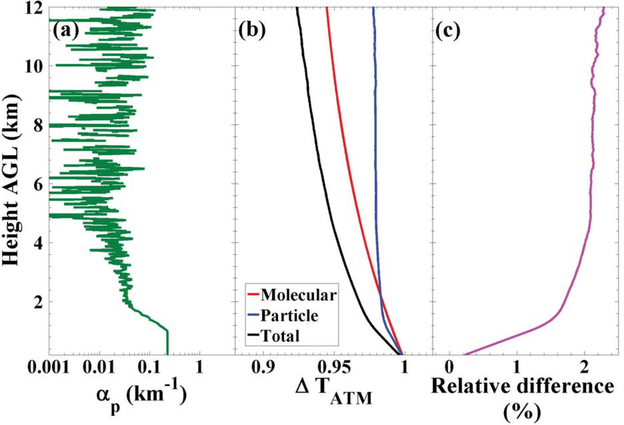
Figure 1(a) Aerosol extinction coefficient (αp). (b) Differential atmospheric transmission (ΔTATM, see Eq. 2): total (black), particles (blue) and molecules (red). (c) Relative difference between differential transmissions when considering and ignoring the contribution of particles to atmospheric transmission.
To calculate the PWV for the Raman lidar, the absolute humidity (or water vapor concentration) is needed. The water vapor concentration can be obtained from the measured WVMR profile, w(z,C), and a computed air density (in g m−3) profile:
with p in hectopascal and T in Kelvin. The pressure and temperature profiles are taken from the GDAS database. The closest four grid points of GDAS model to the location of PollyXT are plotted in Fig. 2. The meteorological data at the grid point of 34.5∘ N, 33∘ E are used in this study. The distance between the grid point and the PollyXT location is 19.7 km.
According to the definition of the WVMR, the water vapor concentration is then given by
Finally, the Raman lidar retrieved precipitable water vapor is calculated with
Considering the blind range for lidar detection, z0 is set at 30 m. z1 is set to 9 km in this study since above this height the amount of water vapor is rather low (Foth et al., 2015).
We compare the temperature and dry air density from GDAS and the simultaneous radiosonde observation to demonstrate the accuracy of the GDAS data in Fig. 3. The details of radiosonde measurements are provided in Sect. 2.3. During CyCARE, 43 radiosondes were launched. In Fig. 3a and b, the temperature from GDAS (red solid line) and the radiosonde (green dashed line), as well as the temperature difference (green solid line in Fig. 3b, 0.064 ± 0.70 ∘C), is shown. It is found that the temperature difference is smaller than 1 ∘C, which agrees with the result from Seifert et al. (2010). The pink solid line in Fig. 3c shows the respective difference for the air density. The modeled air density deviates from the observed data by no more than 0.00062 ± 0.0027 kg m−3 on average. It means that the relative deviation of the dry air density from GDAS and radiosonde data is less than 1 % below 10 km. The blue dotted lines in Fig. 3b and c indicate the ranges of ±1 ∘C and ± 0.005 kg m−3, respectively. In Fig. 3d, the correlation of temperature values from all 43 radiosondes and simultaneous GDAS estimations is plotted. The bias of the radiosonde data in comparison to the GDAS data is 0.23 ∘C and the root-mean-square deviation amounts to 0.87 ∘C. Thus, the temperature and pressure profiles from GDAS are used for the calculation of the dry air density and for the calibration of the Raman lidar water vapor measurements.
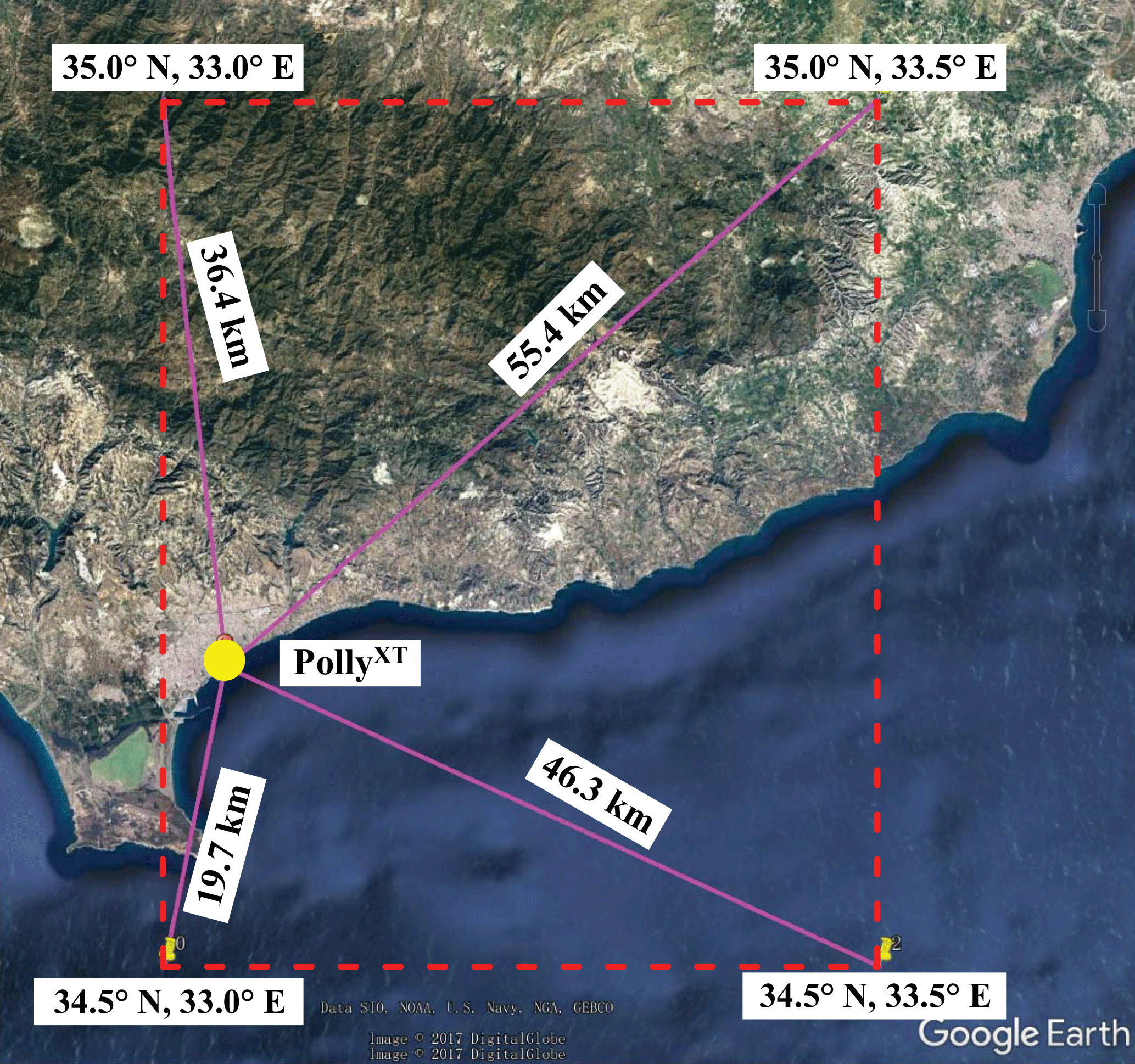
Figure 2The nearest four GDAS grid points around the PollyXT location at Limassol, Cyprus, and the corresponding geographic information. Map: Google Earth (October 2017).
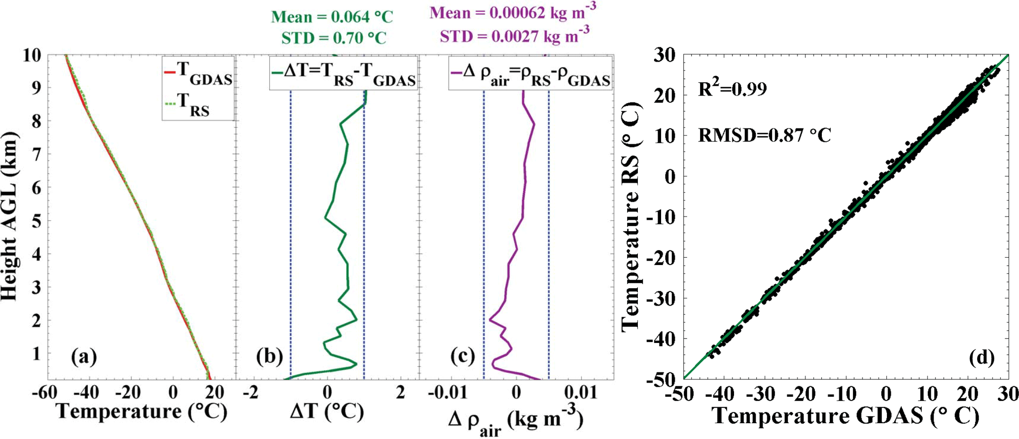
Figure 3(a) Comparison of temperature profiles from the GDAS database and radiosonde observations; (b) the difference between the two temperature values; (c) the respective difference between the dry air density retrieved from GDAS data and from the radiosonde observation measured on 15 April 2017; and (d) the correlation of temperature values from all 43 radiosondes and simultaneous GDAS estimations at the grid point 34.5∘ N, 33∘ E.
2.2 Precipitable water vapor from sun photometer measurements
Ground-based automated sun photometers are globally distributed for providing column-averaged aerosol optical and microphysical properties of particles and the column water vapor content PWV. Most of these systems are operated in the global network AERONET, which takes care of data quality and fast access to the data. The systems usually have channels at the wavelengths of 340, 380, 440, 500, 670, 870 and 1020 nm for the measurement of direct sun, aureole and sky radiances, whereby the channel at 940 nm is used for the retrieval of PWV. In Smirnov et al. (2004), the procedure for retrieving water column abundance from sun photometer observations is discussed. In the 940 nm water absorption band, the response Vw of the sun photometer to irradiance can be calculated by
where τw is the optical thickness arising from broadband continuum type extinction mainly due to molecular (Rayleigh) and particle scattering and water vapor absorption in the 940 nm band. tw denotes the transmission due to water vapor which can be calculated by the air mass m and PWV. V0 is the extraterrestrial voltage. Starting from Eq. (6), PWV from sun photometer can be determined from
where the constants of a and b can be determined by fitting the weighted water vapor transmittance simulated by a radiative transfer model for an instrument-specific filter function. By plotting against , a line with a slope equal to b and an intercept of ln (a) can be fitted (Barreto et al., 2013).
The PWV from sun photometer is available in the AERONET database. According to Holben et al. (2001), the uncertainty of is estimated to be around 10 % caused by the retrieval algorithm and the relatively large uncertainty in the extraterrestrial voltage determined by the Langley method in the 940 nm channel. In Galkin et al. (2011), the same uncertainty value is estimated, which mainly results from errors in instrument calibration.
In this study, the PWV values from the radiosonde and sun photometer observations are compared to estimate the uncertainty in the AERONET PWV values from sun photometer. Twenty daytime measurements with radiosonde and sun photometer are used. Level 2.0 PWV data were used in 11 cases and level 1.5 data had to be used in the remaining 9 cases. The results are shown in Fig. 4. It can be seen that the mean relative difference of PWV measured with sun photometer and radiosonde is 1.07 % ± 4.94 %, which indicates that sun photometer has sufficient accuracy to act as reference instrument in the Raman lidar calibration procedure.
2.3 Water vapor profiles from radiosonde measurements
During the CyCARE campaign, radiosondes of the type VAISALA RS92 were frequently launched at the lidar site in Limassol in April 2017. The radiosonde provides the vertical profiles of relative humidity (%), temperature (∘C), pressure (hPa) and horizontal wind velocity (m s−1) and direction (∘). The measurement uncertainty is 0.2 ∘C in the case of temperatures at a pressure between 100 and 1080 hPa. The absolute uncertainties in the pressure and RH observations are 1 hPa and 5 %, respectively. Vertical profiles of WVMR can be determined as well. Systematic errors of the radiosonde measurements were investigated by Vömel et al. (2007).
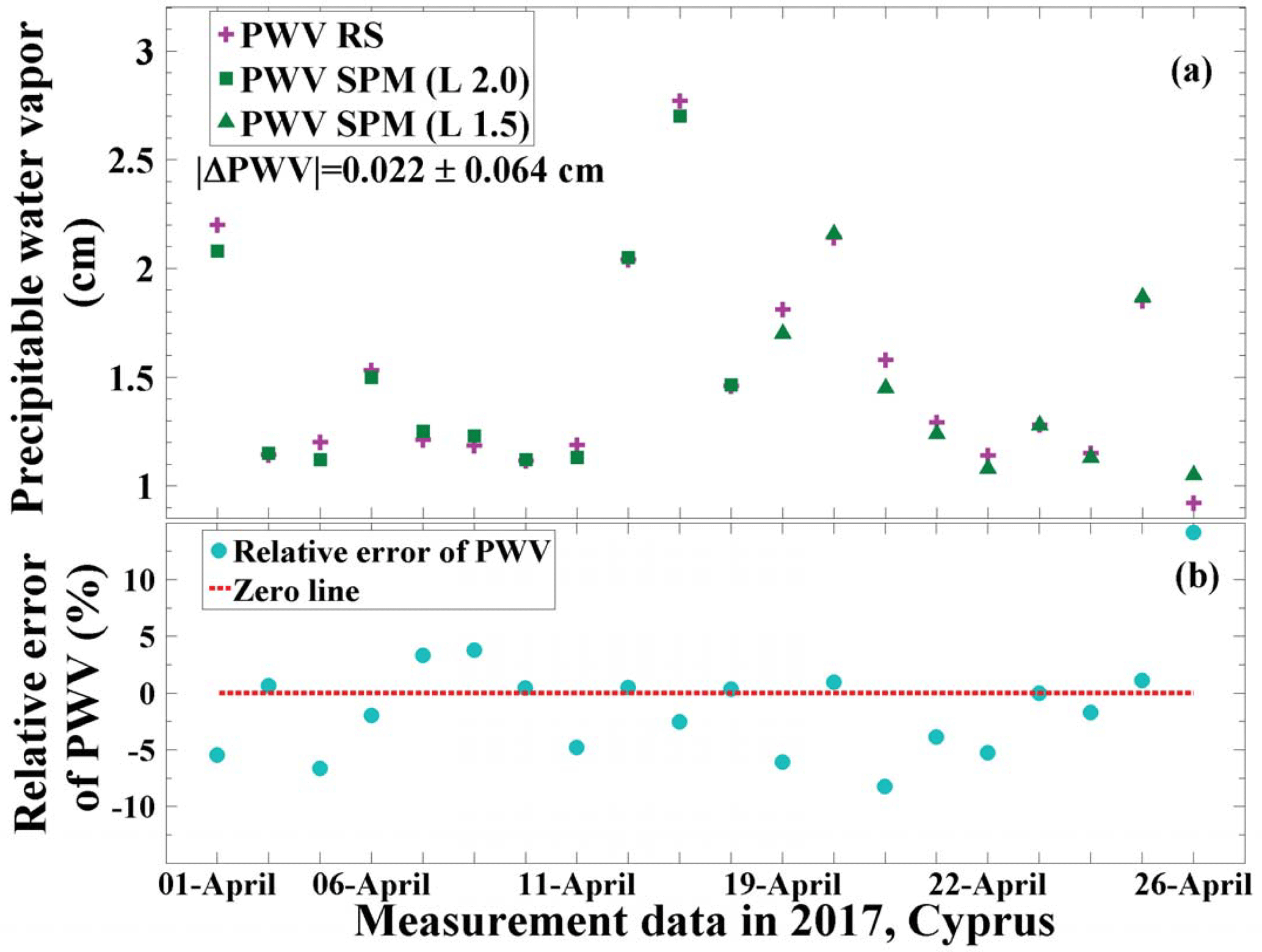
Figure 4(a) Comparison of daytime precipitable water vapor (PWV) measured with radiosonde (RS) and sun photometer (SPM). (b) Relative error of PWV values from SPM measurements.
The calibration constant C in Eq. (2) can be determined by comparing measurements from Raman lidar and co-located sun photometer observations. The flowchart describing the calibration procedure is shown in Fig. 5.
Since sun photometer delivers the PWV or column water vapor content and PollyXT measures the vertical profile of the WVMR, we have to calculate from the lidar measurements by means of Eqs. (3)–(5). The calibration constant C is obtained when the condition
is fulfilled. Because the density of liquid water is approximately 1 g cm−3, the units g cm−2 and centimeters are interchangeable for and (Han et al., 1994).
The total uncertainty of the calibration constant includes instrumental and statistical errors. The relative error of the calibration constant has been determined to about 11 % by taking into account all possible error sources. The more detailed description on uncertainties of the calibration constant is presented in Appendix B.
3.1 Calibration results
The lidar did measure the at nighttime. However, depending on the types of photometers, some of them provide daytime observations while the others (e.g., lunar photometers) could even perform nighttime observations. Thus, two modes of calibration including nighttime–daytime calibration and nighttime calibration are discussed in this study.
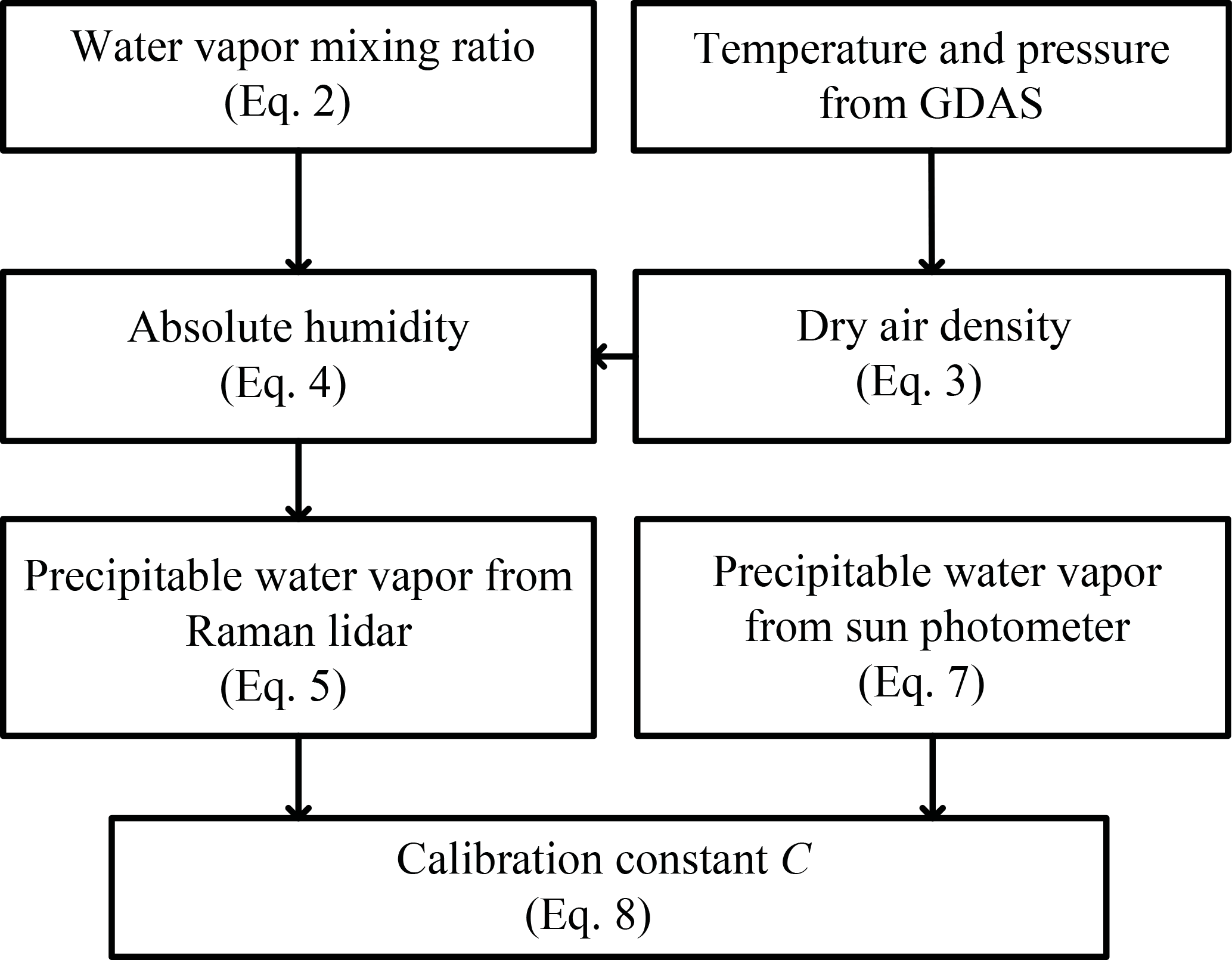
Figure 5Flowchart of the calibration procedure based on co-located sun photometer observations and GDAS data.
3.1.1 Nighttime–daytime calibration
During the CyCARE campaign in April 2017, the sun photometer can measure the at daytime. Nine lidar measurements performed during clear nights are selected for the determination of the calibration constant. The WVMR information from PollyXT measured before dawn (nighttime) and PWV from sun photometer observed at daybreak (daytime) are used for comparison. Only co-located lidar and sun photometer measurements with time differences of less than 1.5 h are considered. Additionally, only cases with very homogeneous atmospheric conditions were used for the calibration. Figure 6 shows an example. The calibration time period is from 02:00 to 04:15 UTC. The temporal development of the range-corrected signal at 1064 nm indicates homogenous atmospheric conditions. In Fig. 6b and c, the WVMR and density are presented as mean values for the time period from 02:00 to 02:30 UTC. These profiles are used. The water vapor concentration (Eq. 4) was calculated from the measured WVMR w(z,C) (Eq. 2). The precipitable water vapor is then calculated by Eq. (5). In this measurement case, the value of the is 0.17⋅C cm while the is 1.17 cm at 04:00 UTC. Therefore, following Eq. (8), the water vapor calibration constant is determined to be 6.88 ± 0.75 g kg−1. Following the same method, the water vapor calibration constants from all nine measurement cases in April are obtained. The results are shown in Fig. 7. From this figure, the determined calibration constant is 6.56 g kg−1 with a total absolute uncertainty (including statistical and instrumental error) of 0.72 g kg−1 and a relative uncertainty of 11 %, respectively. The error analysis is provided in Appendix B.
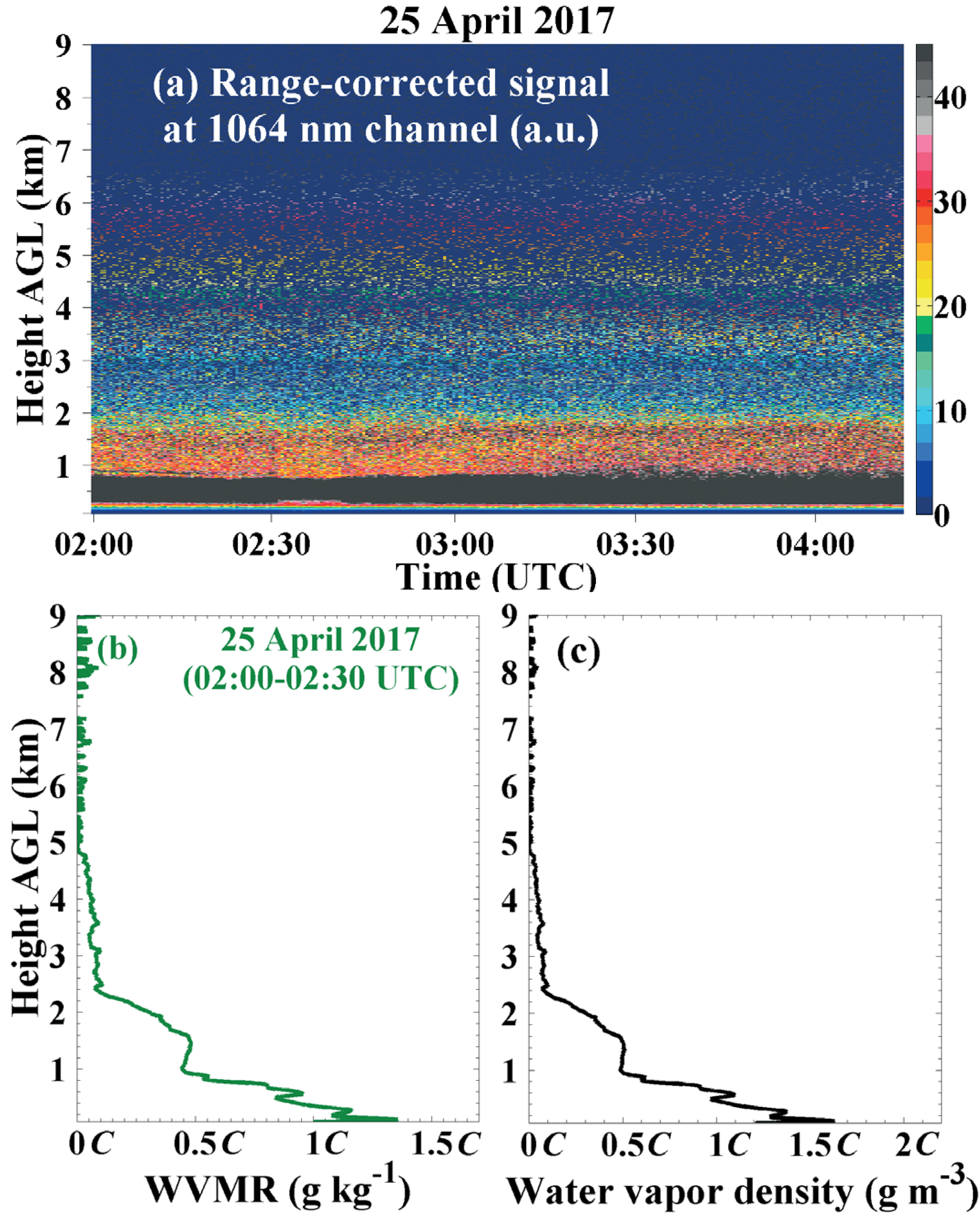
Figure 6(a) Temporal development of the range-corrected signal at 1064 nm, (b) 30 min mean water vapor mixing ratio profile measured on 25 April 2017 from 02:00 to 02:30 UTC, and (c) the corresponding water vapor density profile. Note that the calibration constant C is not yet determined.
3.1.2 Nighttime calibration
The sun and lunar photometer Cimel CE318-T within the pre-campaign of CyCARE in 2015 provides the PWV from moon light measurements at nights, too. Hence, 11 measurements performed during clear nights are selected for the determination of the calibration constant from this campaign. Following the same calibration method, these water vapor calibration constants are shown in Fig. 8. The resulting calibration constant is 6.63 g kg−1 with a total absolute uncertainty (including statistical and instrumental error) of 0.73 g kg−1 and a relative uncertainty of 11 %. These results fit the findings of Sect. 3.1.1.
3.2 Comparisons of calibrated WVMR from lidar with radiosonde measurements
In this section, we compare the calibrated WVMR profiles from the lidar observations with accompanying radiosonde measurements. During CyCARE in April 2017, 43 radiosondes were launched and 19 of them were operated at nighttime and can be used for the comparison. Four representative WVMR profiles of different days are shown in Fig. 9. The solid blue lines indicate the WVMR profiles measured with PollyXT. The dashed red lines denote the WVMR observed with radiosonde. The lidar data are averaged over 30 min. A very good agreement between the lidar and radiosonde profiles was found.
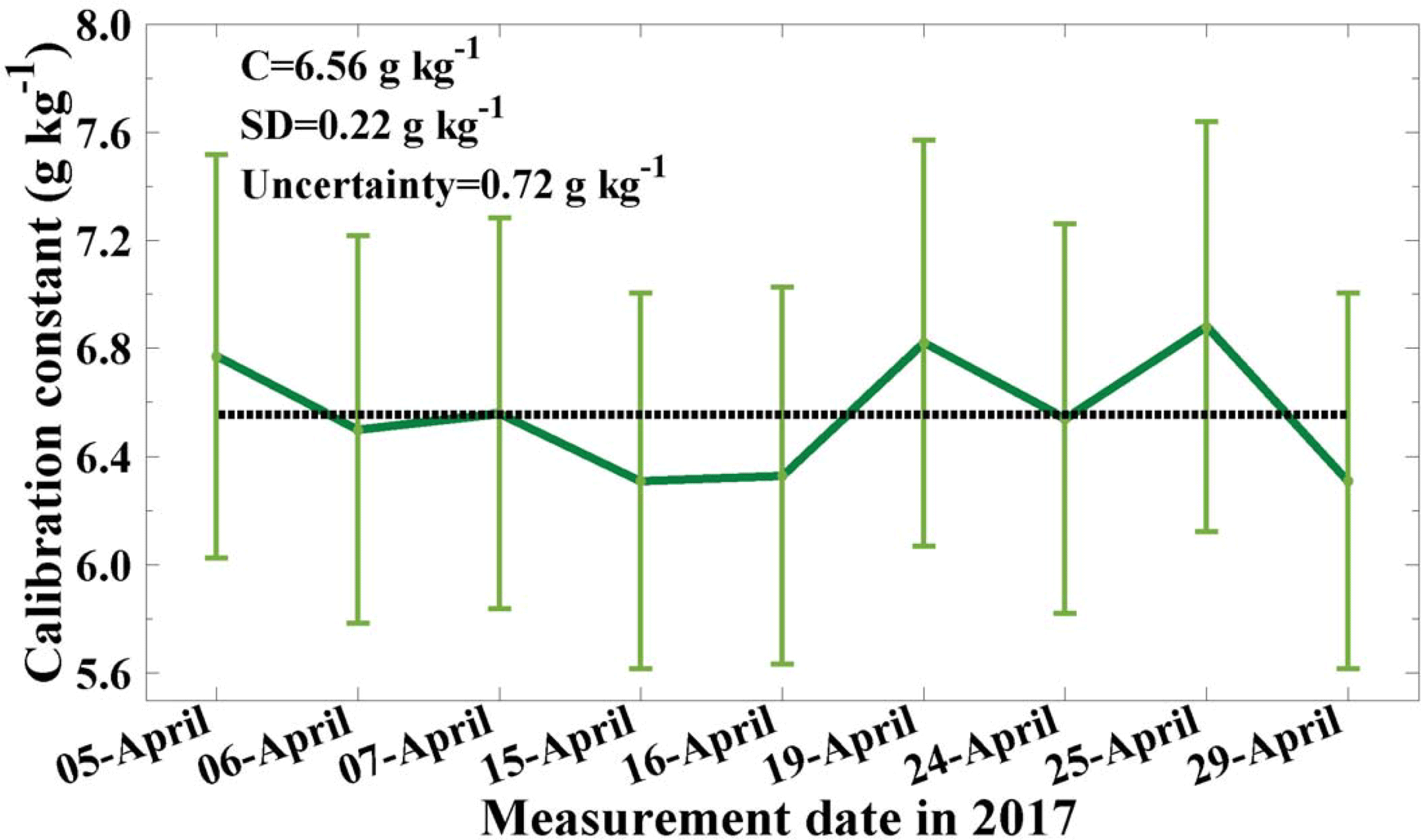
Figure 7Calibration constants (C) determined for nine pairs of lidar and sun photometer observations by using Eq. (8) in the nine selected measurements (thick, green solid line). The error bar shows the overall retrieval error (see Appendix B, Eq. B3). The dotted line shows the mean value of all the nine daily values.
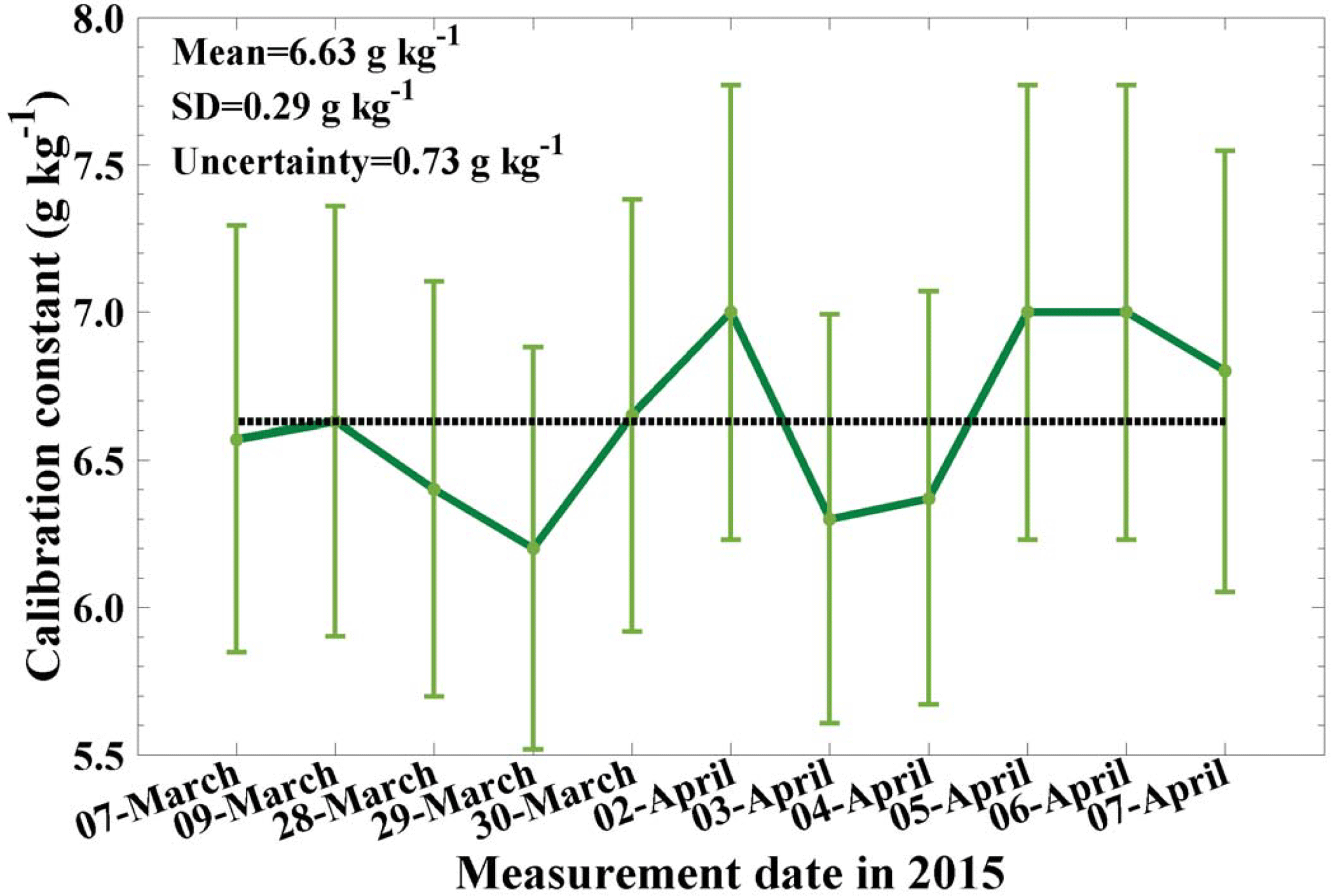
Figure 8Calibration constants (C) determined for 11 pairs of lidar and (sun and) lunar photometer observations by using Eq. (8) in the 11 selected measurements (thick, green solid line). The error bar shows the overall retrieval error (see Appendix B, Eq. B3). The dotted line shows the mean value of all the 11 nighttime calibrations.
By using all of the 19 simultaneous nighttime measurements by lidar and radiosonde, we calculate the WVMR differences between these two observations. In Fig. 10a, the differences are shown as black dots. The mean difference is represented by a blue horizontal line and the value is 0.06 g kg−1. The σ values in this figure denote the standard deviations of the differences. In Fig. 10b, the relationship between the water vapor measurements from PollyXT and radiosonde is shown. Data of the WVMR differences larger than 2σ are not considered. The thresholds ±2σ are shown by the dark green horizontal lines in Fig. 10a as well. After the screening, 95.2 % of data were selected for calculations. The remaining 4.8 % data were also marked with red dots in Fig. 10b and are not used for fitting. According to the results, we can find a slope of 1.01 and a R2 of 0.99, which means that the agreement of WVMR measurements from PollyXT and radiosonde is very good.
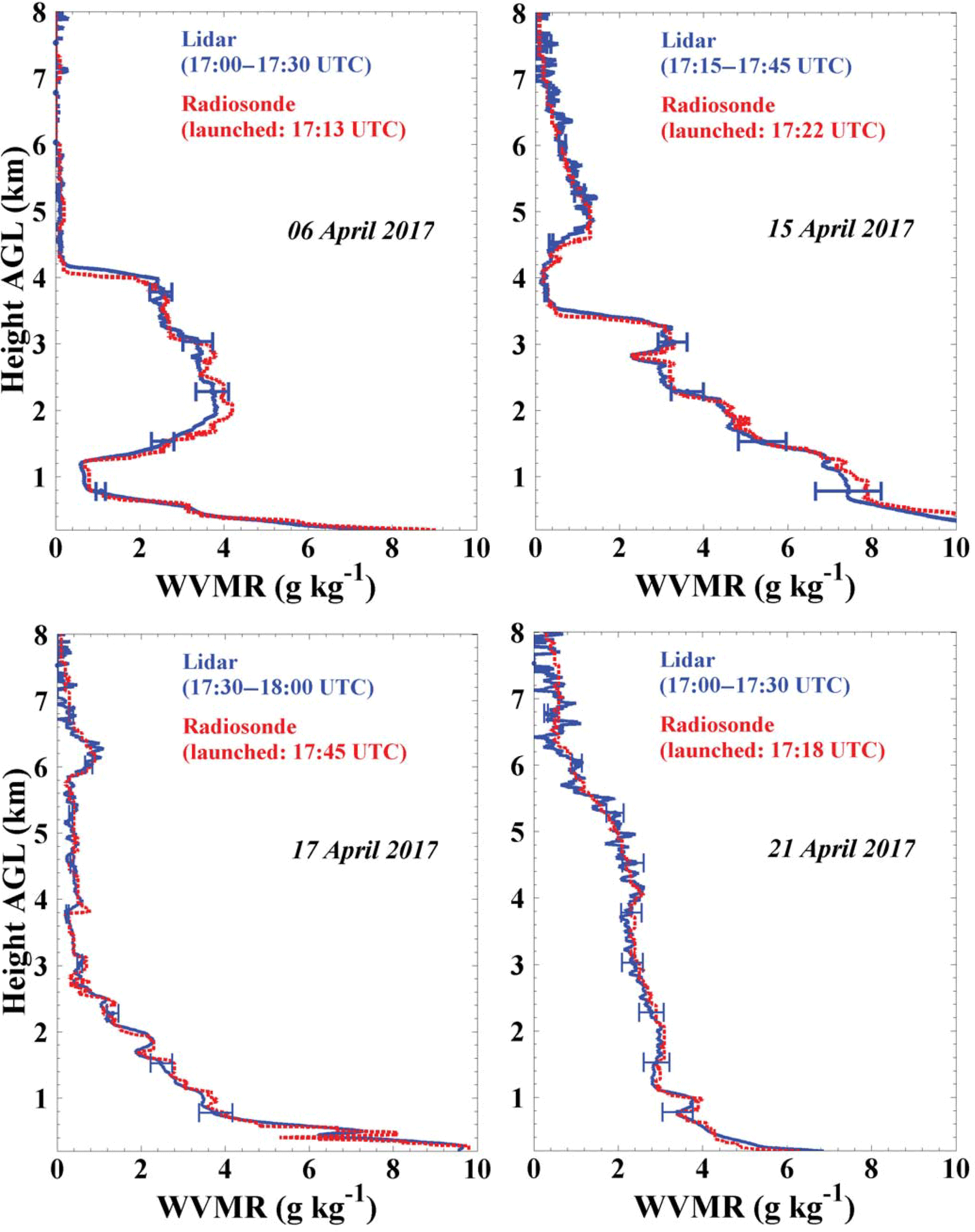
Figure 9Comparison of water vapor mixing ratio profiles measured with PollyXT and radiosonde on 6, 15, 17 and 21 April 2017. Error bars indicate the uncertainty in the water vapor mixing ratios measured with PollyXT.
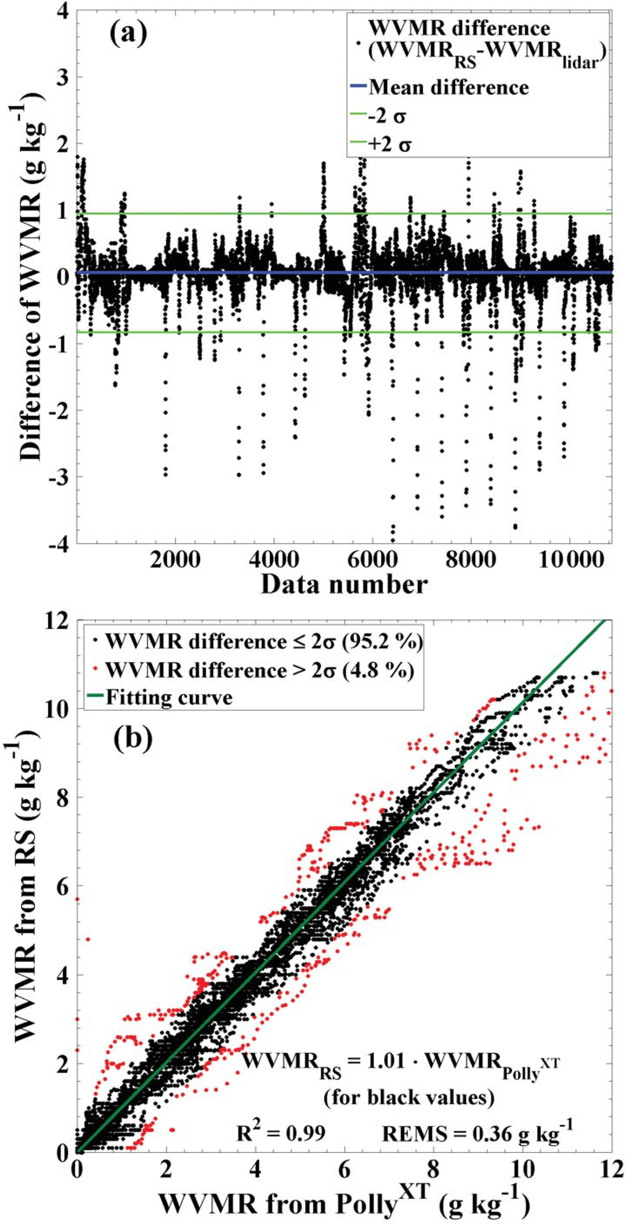
Figure 10(a) Differences between radiosonde and lidar-retrieved water vapor mixing ratios and (b) scatter diagram of lidar WVMR versus radiosonde (RS) WVMR values. All of the 19 simultaneous nighttime measurements with lidar and radiosonde are used. All profile values of the water vapor mixing ratio values between 30 m and 8 km are compared.
By means of Fig. 9 and the scatter diagram in Fig. 10, the quality of the calibration procedure can be well checked. We conclude that the water vapor calibration method based on co-located sun photometer observations and GDAS data is a practical and useful approach to continuously check the calibration of Raman lidar observations of the WVMR.
With the proposed sun-photometer-based calibration method, the WVMR profiles obtained with Raman lidar during the CyCARE campaign were calibrated. Figure 11 presents a measurement from 20 April 2017, 18:00 to 23:59 UTC. In Fig. 11a, the time–height plot of the range-corrected signals at 1064 nm is shown and in Fig. 11b the WVMR is provided. The resolution is 7.5 m and 30 s in Fig. 11a and b; 20 min mean WVMR and RH profiles are presented as well in Fig. 11c and d. Because of the highly accurate GDAS temperature profiles, the respective RH profiles can be determined with good accuracy from the measured WVMR and the saturation WVMR (over liquid water) for the given temperature T(z).
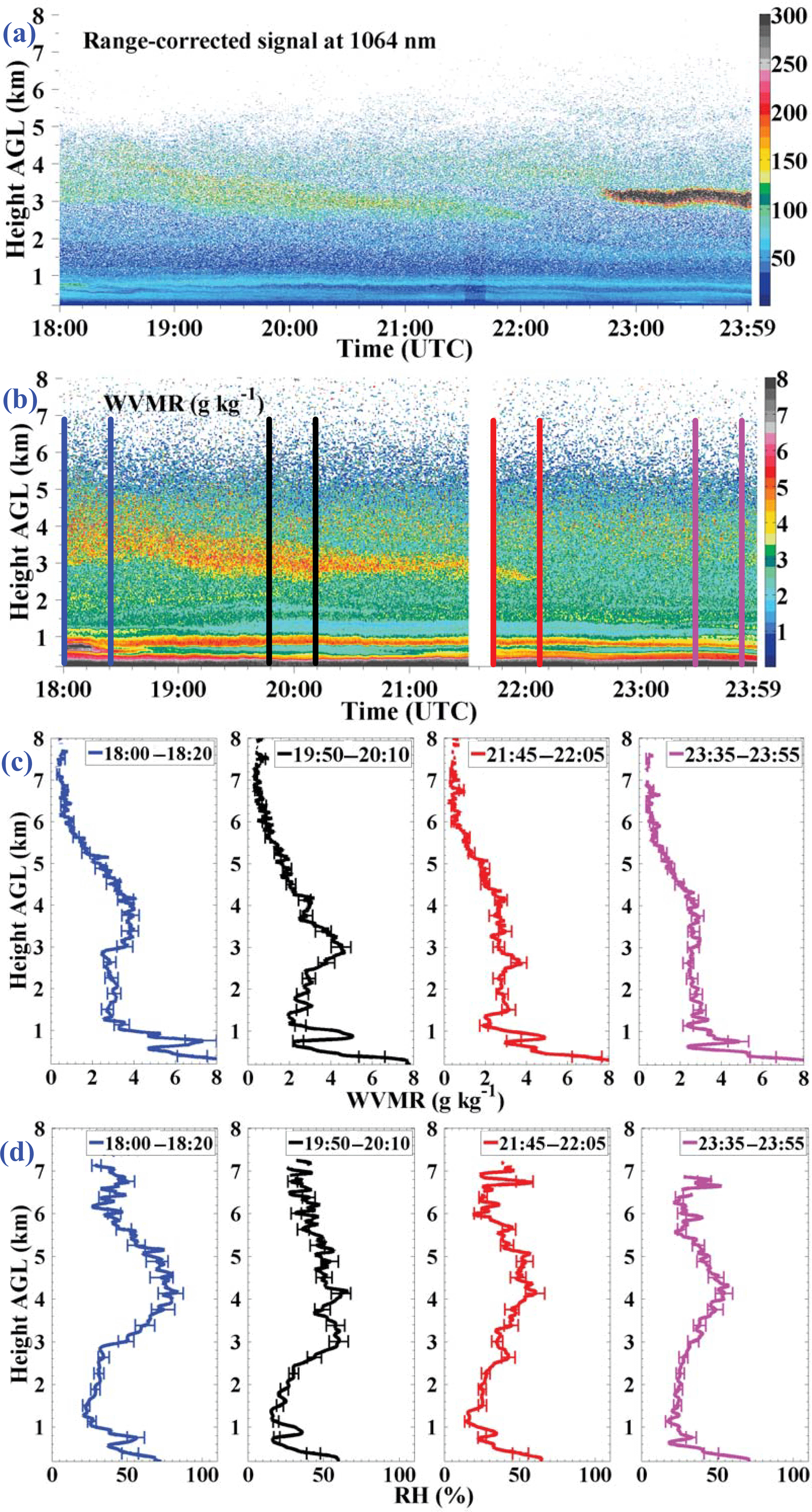
Figure 11Temporal development of the (a) range-corrected signal at 1064 nm and (b) water vapor mixing ratio measured on 20 April 2017. (c) Four water vapor mixing ratio profiles and (d) relative humidity profiles during the periods marked in panel (b) are shown. The temporal resolution for the range-corrected signal and water vapor mixing ratio measurements is 30 s. The integral time of water vapor mixing ratio profiles and relative humidity profiles in panels (c) and (d) is 20 min.
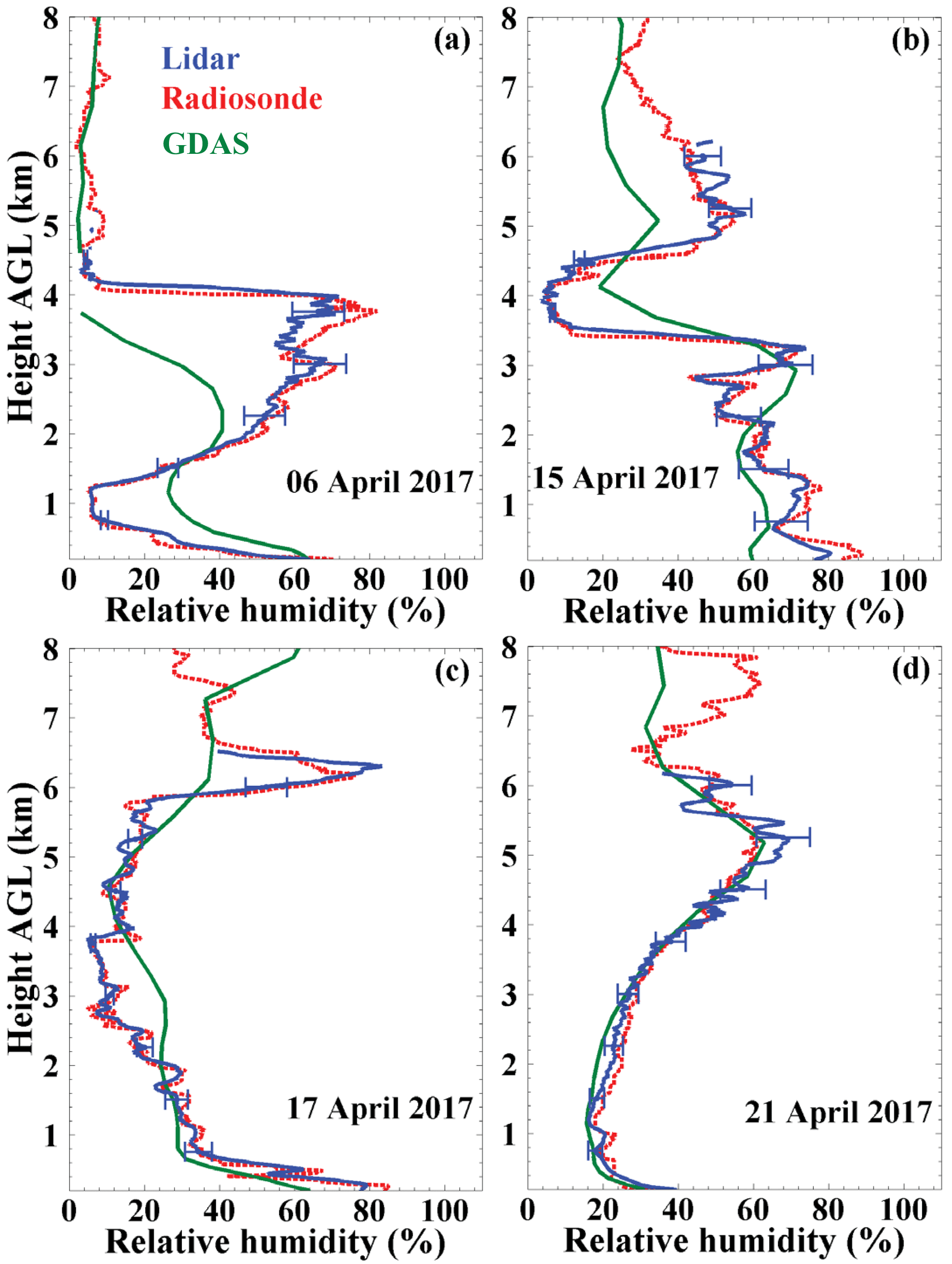
Figure 12Relative humidity (RH) computed from 30 min mean water vapor mixing ratio profiles measured with lidar and by further use of meteorological data from GDAS (blue solid lines). The lidar profiles are compared with radiosonde RH profiles (red dotted profiles) and modeled RH profiles (green curves). The radiosondes were launched during the lidar observations at the lidar field site about 1–2 h after sunset.
As can be seen in Fig. 11a, three layers containing dust are detected above Limassol. The particle depolarization ratios vary from 0.29 to 0.34 in the layers (not shown). The WVMR below and inside the dust layers is retrieved. The white areas above 6 km in Fig. 11b indicate a too low signal-to-noise ratio (SNR), and hence a retrieval of the WVMR is prohibited. Figure 11 shows the humid layers at height < 1 km and the RH close to the ground is larger than 50 %. The pronounced dust layer shows the highest WVMR values in the free troposphere at the heights > 1.5 km and corresponding RH of 50–75 %. Later on, after 22:00 UTC, the free-tropospheric layer is well mixed from 1 to 4.5 km and RH steadily increases with height from 15 % at 1.5 km height to about 50 % at layer top (4.5 km).
In addition, we also present four RH profiles measured with PollyXT on 6, 15, 17 and 21 April in Fig. 12. The lidar-retrieved RH values are again calculated by using the WVMRs from lidar and meteorological data (temperature profile) from GDAS. For comparison, the RH profiles measured with radiosonde (red dashed lines) and estimated by GDAS (green solid lines) are also plotted. The RH profiles from lidar and radiosonde agree very well. The remaining differences may result from the temporal and especially from spatial differences between lidar beam and radiosonde position at height z. The radiosonde drifts with the wind and is typically a few kilometers, 5 and 20 km away from the lidar beam (lidar site) in the lower troposphere, mid-troposphere and upper troposphere, respectively (Seidel et al., 2011). We conclude from the lidar–radiosonde comparison that the RH can be obtained with good accuracy (10–20 %) from the Raman lidar observation of WVMR and temperature profiles from the GDAS datasets.
In this study, the WVMR measured by PollyXT was calibrated by means of co-located AERONET sun photometer observations and GDAS meteorological data. By using the measurement data from the CyCARE campaign, nine measurement cases were selected for the determination of the calibration constant.
The results can be summarized as follows:
-
The PWV data from sun photometer and meteorological data from GDAS can be used for calibrating the water vapor profile from lidar instruments. The method can be used to continuously calibrate the water vapor Raman lidars at AERONET sites. During CyCARE, the water vapor calibration constant of PollyXT was determined to be 6.56 ± 0.72 g kg−1, which indicates a relative uncertainty of 11 %.
-
To validate the water vapor calibration constant determined by applying this method, we compared simultaneous WVMR profile observations with PollyXT and radiosonde. Good agreement between the lidar and the radiosonde measurements was found, also in terms of RH profiles.
-
As an outlook, Raman lidars in combination with GDAS temperature profiles allow us to estimate RH profiles with sufficient accuracy for further use to study relative humidity evolution in the planetary boundary layer and in the free troposphere, e.g., in dust layers or cloud layers (during and before cloud formation), and to study aerosol optical properties obtained from Raman lidar as a function of RH.
AERONET sun photometer data can be downloaded at http://aeronet.gsfc.nasa.gov (refer to Introduction). The GDAS meteorological data can be downloaded at https://www.ready.noaa.gov/READYamet.php (refer to Introduction). Quick looks of the lidar measurements taken in Limassol can be viewed at http://polly.rsd.tropos.de. The lidar and the radiosonde data are available from a server at TROPOS. Please contact Dietrich Althausen (dietrich.althausen@tropos.de) for inquiries.
Whiteman (2003a) showed that the spectra of the Raman signals are temperature dependent. Hence, the molecular backscatter coefficient has to be calculated from
where ΔλR refers to the spectral range over which the Raman vibrational signal is detected and NR(z) is the number density. T(z) is the temperature in Kelvin at the height of z.
Hence we introduce a new function denoted by FR[T(z)], which describes a temperature-dependent function that contains all the temperature dependences in the lidar equation, including backscatter cross section and transmission efficiencies at different wavelengths. This function is expressed by
By this, is changed to . According to Whiteman (2003a, b), the temperature-dependent effect in the troposphere can reach up to 10 % or even more for narrowband Raman water vapor measurement. The exact spectral properties of the water vapor filter strongly affects the transmission intensities of light from water vapor at different temperatures in the atmosphere.
In PollyXT, the central wavelength of the interference filter mounted in the water vapor channel is 407.5 nm with a filter having a FWHM of 1.0 nm, while the filter in the nitrogen channel is 386.7 nm with a FWHM of 0.3 nm. Under this condition, following the results from Whiteman (2003b), the ratio of to is independent of temperature and height. Hence the ratio is a constant and is therefore part of the calibration constant C.
The total error of the calibration constant includes instrumental and statistical errors and can be expressed by
where δx is the uncertainty of the corresponding parameter x. In this study, the statistical error is calculated via
and it is determined to be 1.19 %.
According to Eq. (8) and the error propagation formulas (Bevington and Robinson, 2003), the instrumental error of the calibration constant is calculated via
where Rw is the ratio of to and RF is the ratio of to . The error of the calibration constant is related to the error of Rw, RF and ΔTATM in the calibration measurements. The error of ΔTATM is introduced in Sect. 2.1. Since the ratio RF is a constant, the error caused by RF will not be taken into consideration.
As for Rw, the uncertainty can be calculated by
The SNR and SNR are the signal to noise ratios of the water vapor Raman channel and the nitrogen Raman channel, respectively. According to Heese et al. (2010), the SNR(z,λR) of the backscattered signal detected by PollyXT is determined via
where refers to the background term of water vapor Raman channel or nitrogen Raman channel.
Based on the error analysis described above, the uncertainty of calibration constant is about 11 %. It should be emphasized that once the total uncertainty was determined, the calibration constant will not be influenced by the Rw, RF and ΔTATM in a regular measurement (not for calibration) and they are independent of each other. According to the error propagation formulas, the relative error of the water vapor mixing ratio can be calculated from Eq. (2) as
The authors declare that they have no conflict of interest.
The authors acknowledge funding from the European Union's Horizon 2020
research and innovation programme under grant agreement nos. 654109
(ACTRIS-2), 690133 (GEO-CRADLE) and 763643 (EXCELSIOR) and previously
from the European Union Seventh Framework Programme (FP7/2007–2013) under
grant agreement no. 262254 (ACTRIS) and 603445 (BACCHUS). The authors thank
the Cyprus University of Technology and Remote Sensing and Geo-Environment
Lab (ERATOSTHENES Research Centre) for their support during CyCARE. Guangyao
Dai appreciates the support from the Chinese Scholarship Council (CSC) to
conduct this research under the CSC no. 201606330022.
Edited by: Vassilis Amiridis
Reviewed by: two
anonymous referees
Althausen, D., Engelmann, R., Baars, H., Heese, B., Ansmann, A., Müller, D., and Komppula, M.: Portable Raman Lidar PollyXT for Automated Profiling of Aerosol Backscatter, Extinction, and Depolarization, J. Atmos. Ocean. Tech., 26, 2366–2378, https://doi.org/10.1175/2009JTECHA1304.1, 2009. a
Ansmann, A., Riebesell, M., Wandinger, U., Weitkamp, C., and Michaelis, W.: Tropospheric water vapor measurement by Raman lidar: atmospheric extinction correction, in: Proceedings of Fifteenth International Laser Radar Conference (part 1), Tomsk, USSR: Institute of Atmospheric Optics, 256–259, 1990. a
Ansmann, A., Riebesell, M. A., Wandinger, U., Weitkamp, C., Voss, E., Lahmann, W., and Michaelis, W.: Combined raman elastic-backscatter LIDAR for vertical profiling of moisture, aerosol extinction, backscatter, and LIDAR ratio, App. Phys., 55, 18–28, https://doi.org/10.1007/BF00348608, 1992. a, b
Barreto, A., Cuevas, E., Damiri, B., Romero, P. M., and Almansa, F.: Column water vapor determination in night period with a lunar photometer prototype, Atmos. Meas. Tech., 6, 2159–2167, https://doi.org/10.5194/amt-6-2159-2013, 2013. a, b
Bengtsson, L., Andrae, U., Aspelien, T., Batrak, Y., Calvo, J., de Rooy, W., Gleeson, E., Hansen-Sass, B., Homleid, M., Hortal, M., Ivarsson, K.-I., Lenderink, G., Niemelä, S., Nielsen, K., Onvlee, J., Rontu, L., Samuelsson, P., Santos-Munoz, D., Subias, A., Tijm, S., Toll, V., Yang, X., and Koltzow, M.: The HARMONIE–AROME Model Configuration in the ALADIN–HIRLAM NWP System, Mon. Weather Rev., 145, 1919–1935, https://doi.org/10.1175/MWR-D-16-0417.1, 2017. a
Bevington, P. and Robinson, D.: Data Reduction and Error Analysis for the Physical Sciences, McGraw-Hill; New York, 2003. a
Bucholtz, A.: Rayleigh-scattering calculations for the terrestrial atmosphere, Appl. Opt., 34, 2765–2773, https://doi.org/10.1364/AO.34.002765, 1995. a
Cooney, J.: Remote measurements of atmospheric water vapor profiles using the Raman component of laser backscatter, J. Appl. Meteor., 9, 182–184, https://doi.org/10.1175/1520-0450(1970)009<0182:RMOAWV>2.0.CO;2, 1970. a
David, L., Bock, O., Thom, C., Bosser, P., and Pelon, J.: Study and mitigation of calibration factor instabilities in a water vapor Raman lidar, Atmos. Meas. Tech., 10, 2745–2758, https://doi.org/10.5194/amt-10-2745-2017, 2017. a
Engelmann, R., Kanitz, T., Baars, H., Heese, B., Althausen, D., Skupin, A., Wandinger, U., Komppula, M., Stachlewska, I. S., Amiridis, V., Marinou, E., Mattis, I., Linné, H., and Ansmann, A.: The automated multiwavelength Raman polarization and water-vapor lidar Polly𝙓𝙏: the neXT generation, Atmos. Meas. Tech., 9, 1767–1784, https://doi.org/10.5194/amt-9-1767-2016, 2016. a, b
Ferrare, R., Turner, D., Clayton, M., Schmid, B., Redemann, J., Covert, D., Elleman, R., Ogren, J., Andrews, E., and Goldsmith, J. E. M. G. a.: Evaluation of daytime measurements of aerosols and water vapor made by an operational Raman lidar over the Southern Great Plains, J. Geophys. Res.-Atmos., 111, D05S08, https://doi.org/10.1029/2005JD005836, 2006. a
Filioglou, M., Nikandrova, A., Niemelä, S., Baars, H., Mielonen, T., Leskinen, A., Brus, D., Romakkaniemi, S., Giannakaki, E., and Komppula, M.: Profiling water vapor mixing ratios in Finland by means of a Raman lidar, a satellite and a model, Atmos. Meas. Tech., 10, 4303–4316, https://doi.org/10.5194/amt-10-4303-2017, 2017. a
Foth, A., Baars, H., Di Girolamo, P., and Pospichal, B.: Water vapour profiles from Raman lidar automatically calibrated by microwave radiometer data during HOPE, Atmos. Chem. Phys., 15, 7753–7763, https://doi.org/10.5194/acp-15-7753-2015, 2015. a, b, c, d
Galkin, V. D., Immler, F., Alekseeva, G. A., Berger, F.-H., Leiterer, U., Naebert, T., Nikanorova, I. N., Novikov, V. V., Pakhomov, V. P., and Sal'nikov, I. B.: Analysis of the application of the optical method to the measurements of the water vapor content in the atmosphere – Part 1: Basic concepts of the measurement technique, Atmos. Meas. Tech., 4, 843–856, https://doi.org/10.5194/amt-4-843-2011, 2011. a, b
Halthore, R. N., Eck, T. F., Holben, B. N., and Markham, B. L.: Sun photometric measurements of atmospheric water vapor column abundance in the 940-nm band, J. Geophys. Res., 102, 4343–4352, https://doi.org/10.1029/96JD03247, 1997. a
Han, Y., Snider, J., Westwater, E., Melfi, S., and Ferrare, R.: Observations of water vapor by ground-based microwave radiometers and Raman lidar, J. Geophys. Res.-Atmos., 99, 18695–18702, https://doi.org/10.1029/94JD01487, 1994. a
Heese, B., Flentje, H., Althausen, D., Ansmann, A., and Frey, S.: Ceilometer lidar comparison: backscatter coefficient retrieval and signal-to-noise ratio determination, Atmos. Meas. Tech., 3, 1763–1770, https://doi.org/10.5194/amt-3-1763-2010, 2010. a
Held, I. and Soden, B.: Water vapor Feedback and Global Warming, Annu. Rev. Energy Environ., 25, 441–475, https://doi.org/10.1146/annurev.energy.25.1.441, 2000. a
Holben, B. N., Eck, T. F., Slutsker, I., Tanré, D., Buis, J. P., Setzer, A., E., V., Reagan, J. A., Kaufman, Y. J., Nakajima, T., Lavenu, F., Jankowiak, I., and Smirnov, A.: AERONET – A Federated Instrument Network and Data Archive for Aerosol Characterization, Remote Sens. Environ., 66, 1–16, https://doi.org/10.1016/S0034-4257(98)00031-5, 1998. a
Holben, B. N., Tanré, D., Smirnov, A., Eck, T. F., Slutsker, I., Abuhassan, N., Newcomb, W. W., Schafer, J. S., Chatenet, B., Lavenu, F., Kaufman, Y. J., Castle, J. V., Setzer, A., Markham, B., Clark, D., Frouin, R., Halthore, R., Karneli, A., O'Neill, N. T., Pietras, C., Pinker, R. T., Voss, K., and Zibordi, G.: An emerging ground-based aerosol climatology: Aerosol optical depth from AERONET, J. Geophys. Res.-Atmos., 106, 12067–12097, https://doi.org/10.1029/2001JD900014, 2001. a
Leblanc, T. and McDermid, I. S.: Accuracy of Raman lidar water vapor calibration and its applicability to long-term measurements, Appl. Opt., 47, 5592–5603, https://doi.org/10.1364/AO.47.005592, 2008. a
Leblanc, T., McDermid, I. S., and Walsh, T. D.: Ground-based water vapor raman lidar measurements up to the upper troposphere and lower stratosphere for long-term monitoring, Atmos. Meas. Tech., 5, 17–36, https://doi.org/10.5194/amt-5-17-2012, 2012. a
Madonna, F., Amodeo, A., Boselli, A., Cornacchia, C., Cuomo, V., D'Amico, G., Giunta, A., Mona, L., and Pappalardo, G.: CIAO: the CNR-IMAA advanced observatory for atmospheric research, Atmos. Meas. Tech., 4, 1191–1208, https://doi.org/10.5194/amt-4-1191-2011, 2011. a, b
Mattis, I., Ansmann, A., Althausen, D., Jaenisch, V., Wandinger, U., Müller, D., Arshinov, Y. F., Bobrovnikov, S. M., and Serikov, I. B.: Relative-humidity profiling in the troposphere with a Raman lidar, Appl. Opt., 41, 6451–6462, https://doi.org/10.1364/AO.41.006451, 2002. a
Melfi, S., Lawrence Jr., J., and McCormick, M.: Observation of Raman scattering by water vapor in the atmosphere, Appl. Phys. Lett., 15, 295–297, https://doi.org/10.1063/1.1653005, 1969. a
Parkinson, C. L.: Aqua: An Earth-observing satellite mission to examine water and other climate variables, IEEE T. Geosci. Remote, 41, 173–183, https://doi.org/10.1109/TGRS.2002.808319, 2003. a
Pérez-Ramírez, D., Whiteman, D. N., Smirnov, A., Lyamani, H., Holben, B. N., Pinker, R., Andrade, M., and Alados-Arboledas, L.: Evaluation of AERONET precipitable water vapor versus microwave radiometry, GPS, and radiosondes at ARM sites, J. Geophys. Res.-Atmos., 119, 9596–9613, https://doi.org/10.1002/2014JD021730, 2014. a
Schmid, B., Livingston, J. M., Russell, P. B., Durkee, P. A., Jonsson, H. H., Collins, D. R., Flagan, R. C., Seinfeld, J. H., Gassó, S., Hegg, D. A., Öström, E., Noone, K. J., Welton, E. J., Voss, K. J., Gordon, H. R., Formenti, P., and Andreae, M. O.: Clear-sky closure studies of lower tropospheric aerosol and water vapor during ACE-2 using airborne sunphotometer, airborne in-situ, space-borne, and ground-based measurements, Tellus B, 52, 568–593, https://doi.org/10.3402/tellusb.v52i2.16659, 2000. a
Seidel, D. J., Sun, B., Pettey, M., and Reale, A.: Global radiosonde balloon drift statistics, J. Geophys. Res.-Atmos., 116, D07102, https://doi.org/10.1029/2010JD014891, 2011. a
Seifert, P., Ansmann, A., Mattis, I., Wandinger, U., Tesche, M., Engelmann, R., Müller, D., Pérez, C., and Haustein, K.: Saharan dust and heterogeneous ice formation: Eleven years of cloud observations at a central European EARLINET site, J. Geophys. Res.-Atmos., 115, D20201, https://doi.org/10.1029/2009JD013222, 2010. a
Seity, Y., Brousseau, P., Malardel, S., Hello, G., Bénard, P., Bouttier, F., Lac, C., and Masson, V.: The AROME-France convective-scale operational model, Mon. Weather Rev., 139, 976–991, https://doi.org/10.1175/2010MWR3425.1, 2011. a
Sherlock, V., Garnier, A., Hauchecorne, A., and Keckhut, P.: Implementation and validation of a Raman lidar measurement of middle and upper tropospheric water vapor, Appl. Opt., 38, 5838–5850, https://doi.org/10.1364/AO.38.005838a, 1999a. a
Sherlock, V., Hauchecorne, A., and Lenoble, J.: Methodology for the independent calibration of Raman backscatter water-vapor lidar systems, Appl. Opt., 38, 5816–5837, https://doi.org/10.1364/AO.38.005816, 1999b. a
Smirnov, A., Holben, B. N., Lyapustin, A., Slutsker, I., and Eck, T. F.: AERONET processing algorithms refinement, in: AERONET Workshop, El Arenosillo, Spain, 10–14, available at: https://aeronet.gsfc.nasa.gov/new_web/spain2004/presentations/Smirnov_Algorithm.ppt (last access: 30 April 2018), 2004. a, b
Tompkins, A. M.: A Prognostic Parameterization for the Subgrid-Scale Variability of Water Vapor and Clouds in Large-Scale Models and Its Use to Diagnose Cloud Cover, J. Atmos. Sci., 59, 1917–1942, https://doi.org/10.1175/1520-0469(2002)059<1917:APPFTS>2.0.CO;2, 2002. a
Torres, B., Cachorro, V. E., Toledano, C., Ortiz de Galisteo, J. P., Berjón, A., De Frutos, A., Bennouna, Y., and Laulainen, N.: Precipitable water vapor characterization in the Gulf of Cadiz region (southwestern Spain) based on Sun photometer, GPS, and radiosonde data, J. Geophys. Res.-Atmos., 115, D18103, https://doi.org/10.1029/2009JD012724, 2010. a
Totems, J. and Chazette, P.: Calibration of a water vapour Raman lidar with a kite-based humidity sensor, Atmos. Meas. Tech., 9, 1083-1094, https://doi.org/10.5194/amt-9-1083-2016, 2016. a
Twomey, S.: Aerosols, clouds and radiation, Atmos. Environ., 25, 2435–2442, https://doi.org/10.1016/0960-1686(91)90159-5, 1991. a
Vaughan, G., Wareing, D. P., Thomas, L., and Mitev, V.: Humidity measurements in the free troposphere using Raman backscatter, Q. J. Roy. Meteor. Soc., 114, 1471–1484, https://doi.org/10.1002/qj.49711448406, 1988. a
Venable, D. D., Whiteman, D. N., Calhoun, M. N., Dirisu, A. O., Connell, R. M., and Landulfo, E.: Lamp mapping technique for independent determination of the water vapor mixing ratio calibration factor for a Raman lidar system, Appl. Opt., 50, 4622–4632, https://doi.org/10.1364/AO.50.004622, 2011. a
Vladutescu, D. V., Wu, Y., Charles, L., Gross, B., Moshary, F., and Ahmed, S.: Analyses of Raman lidar calibration techniques based on water vapor mixing ratio measurements, WSEAS Trans. Syst., 6, 651, available at: https://www.researchgate.net/profile/Viviana_Vladutescu/publication/229010464_Analyses_of_Raman_lidar_calibration_techniques_based_on_water_vapor_mixing_ratio_measurements/links/0fcfd509454644c708000000.pdf (last access: 30 April 2018), 2007. a
Vömel, H., Selkirk, H., Miloshevich, L., Valverde-Canossa, J., Valdés, J., Kyrö, E., Kivi, R., Stolz, W., Peng, G., and Diaz, J. A.: Radiation dry bias of the Vaisala RS92 humidity sensor, J. Atmos. Ocean. Tech., 24, 953–963, https://doi.org/10.1175/JTECH2019.1, 2007. a
Wandinger, U.: Raman lidar, in: Lidar: Range-Resolved Optical Remote Sensing of the Atmosphere, edited by: Weitkamp, C., Springer Series in Optical Sciences, Springer, 102, 241–271, https://doi.org/10.1007/b106786, 2005. a, b
Whiteman, D. N.: Examination of the traditional Raman lidar technique. I. Evaluating the temperature-dependent lidar equations, Appl. Opt., 42, 2571–2592, https://doi.org/10.1364/AO.42.002571, 2003a. a, b, c
Whiteman, D. N.: Examination of the traditional Raman lidar technique. II. Evaluating the ratios for water vapor and aerosols, Appl. Opt., 42, 2593–2608, https://doi.org/10.1364/AO.42.002593, 2003b. a, b, c, d
Whiteman, D. N., Melfi, S. H., and Ferrare, R. A.: Raman lidar system for the measurement of water vapor and aerosols in the Earth's atmosphere, Appl. Opt., 31, 3068–3082, https://doi.org/10.1364/AO.31.003068, 1992. a
Whiteman, D. N., Venable, D., and Landulfo, E.: Comments on “Accuracy of Raman lidar water vapor calibration and its applicability to long-term measurements”, Appl. Opt., 50, 2170–2176, https://doi.org/10.1364/AO.50.002170, 2011. a
- Abstract
- Introduction
- Water vapor measurements with Raman lidar, sun photometer and radiosonde
- Calibrations of water vapor Raman lidar measurements
- Examples of WVMR and RH measurements
- Conclusions
- Data availability
- Appendix A: Temperature dependence of Raman spectra
- Appendix B: Error analysis of calibration constant and WVMR
- Competing interests
- Acknowledgements
- References