A novel method for calculating ambient aerosol liquid water content based on measurements of a humidified nephelometer system

Water condensed on ambient aerosol particles plays significant roles in atmospheric environment, atmospheric chemistry and climate. Before now, no instruments were available for real-time monitoring of ambient aerosol liquid water contents (ALWCs). In this paper, a novel method is proposed to calculate ambient ALWC based on measurements of a three-wavelength humidified nephelometer system, which measures aerosol light scattering coefficients and backscattering coefficients at three wavelengths under dry state and different relative humidity (RH) conditions, providing measurements of light scattering enhancement factor f(RH). The proposed ALWC calculation method includes two steps: the first step is the estimation of the dry state total volume concentration of ambient aerosol particles, V_a(dry), with a machine learning method called random forest model based on measurements of the “dry” nephelometer. The estimated V_a(dry) agrees well with the measured one. The second step is the estimation of the volume growth factor Vg(RH) of ambient aerosol particles due to water uptake, using f(RH) and the Ångström exponent. The ALWC is calculated from the estimated V_a(dry) and Vg(RH). To validate the new method, the ambient ALWC calculated from measurements of the humidified nephelometer system during the Gucheng campaign was compared with ambient ALWC calculated from ISORROPIA thermodynamic model using aerosol chemistry data. A good agreement was achieved, with a slope and intercept of 1.14 and −8.6 µm³ cm⁻³ (r² = 0.92), respectively. The advantage of this new method is that the ambient ALWC can be obtained solely based on measurements of a three-wavelength humidified nephelometer system, facilitating the real-time monitoring of the ambient ALWC and promoting the study of aerosol liquid water and its role in atmospheric chemistry, secondary aerosol formation and climate change.

1 Introduction

Atmospheric aerosol particles play significant roles in atmospheric environment, climate, human health and the hydrological cycle and have received much attention in recent decades. One of the most important constituents of ambient atmospheric aerosol is liquid water. The content of condensed water on ambient aerosol particles depends mostly on the aerosol hygroscopicity and the ambient relative humidity (RH). Results of previous studies demonstrate that liquid water contributes greatly to the total mass of ambient aerosol particles when the ambient RH is higher than 60 % (Bian et al., 2014). Aerosol liquid water also has large impacts on aerosol optical properties and aerosol radiative effects (Tao et al., 2014; Kuang et al., 2016). Liquid water condensed on aerosol particles can also serves as a site for multiphase reactions which perturb local chemistry and further influence the aging processes of aerosol particles (Martin, 2000). Recent studies have shown that aerosol liquid water serves as a reactor, which can efficiently transform sulfur dioxide to sulfate during haze events, aggravating atmospheric environment in the North China Plain (NCP) (Wang et al., 2016; Cheng et al., 2016). Hence, to gain more insight into the role of aerosol liquid water in atmospheric chemistry, aerosol aging processes and aerosol optical properties, the real-time monitoring of ambient aerosol liquid water content (ALWC) is of crucial importance.

Few techniques are currently available for measuring the ALWC. The humidified tandem differential mobility analyser systems (HTDMAs) are useful tools and widely used to measure hygroscopic growth factors of ambient aerosol particles (Rader and McMurry, 1986; Wu et al., 2016; Meier et al., 2009). Hygroscopicity parameters retrieved from measurements of HTDMAs can be used to calculate the volume of liquid water. Nevertheless, HTDMAs cannot be used to measure the total aerosol water volume, because they are not capable of measuring the hygroscopic properties of the entire aerosol population. With size distributions of aerosol particles in their ambient state and dry state, the aerosol water volume can be estimated. Engelhart et al. (2011) deployed the Dry-Ambient Aerosol Size Spectrometer to measure the aerosol liquid water content and volume growth factor of fine particulate matter. This system provides only aerosol water content of aerosol particles within a certain size range (particle diameter less than 500 nm, for the setup of Engelhart et al., 2011). In addition, in conjunction with aerosol thermodynamic equilibrium models, ALWC can also be estimated with detailed aerosol chemical information. However, simulations of aerosol hygroscopicity and phase state by using thermodynamic equilibrium models are still very complicated even under the thermodynamic equilibrium hypothesis and these models may cause large bias when used for estimating ALWC (Bian et al., 2014).

The idea of using the humidified nephelometer system for the study of aerosol hygroscopicity had already been proposed early on by Covert et al. (1972). The instrument measures aerosol light scattering coefficient (σ_sp) under dry state and different RH conditions, providing information on the aerosol light scattering enhancement factor f(RH). One advantage of this method is that it has a fast response time and continuous measurements can be made, facilitating the monitoring of changes in ambient conditions. Another advantage of this method is that it provides information on the overall aerosol hygroscopicity of the entire aerosol population (Kuang et al., 2017). Measured σ_sp of aerosol particles in dry state and f(RH) vary strongly with parameters of particle number size distribution (PNSD), making it difficult to directly link them with the dry state aerosol particle volume (V_a(dry)) and the volume growth factor Vg(RH) of the entire aerosol population. So far, the ALWC could not be directly estimated based solely on measurements of the humidified nephelometer system. Several studies have shown that given the PNSDs at dry state, an iterative algorithm together with the Mie theory can be used to calculate an overall aerosol hygroscopic growth factor g(RH) based on measurements of f(RH) (Zieger et al., 2010; Fierz-Schmidhauser et al., 2010). In such an iterative algorithm, the g(RH) is assumed to be independent of the aerosol diameter. Thus, ALWC at different RH levels can be calculated based on derived g(RH) and the measured PNSD. This method not only requires additional measurements of PNSD, but also may result in significant deviations of the estimated ALWC, because g(RH) should be a function of aerosol diameter rather than a constant value. Another method, which directly connects f(RH) to Vg(RH) (Vg(RH) = f(RH)^1.5), is also used for predicting ALWC based on measurements of the humidified nephelometer system and mass concentrations of dry aerosol particles (Guo et al., 2015). This method assumes that the average scattering efficiency of aerosol particles at dry state and different RH conditions are the same and requires additional measurements of PNSD or mass concentrations of dry aerosol particles (Guo et al., 2015). However, the scattering efficiency of aerosol particles varies with particle diameters, which will change under ambient conditions due to aerosol hygroscopic growth.

In this paper, we propose a novel method to calculate the ALWC based only on measurements of a humidified nephelometer system. The proposed method includes two steps. The first step is calculating V_a(dry) based on measurements of the “dry” nephelometer using a machine learning method called random forest model. With measurements of PNSD and BC, the six parameters measured by the nephelometer can be simulated using the Mie theory and the V_a(dry) can also be calculated based on PNSD. Therefore, the random forest model can be trained with only the regional historical datasets of PNSD and BC. In this study, datasets of PNSD and BC measured from multiple sites are used in the machine learning model to characterise a regional aerosol and these datasets have covered a wide range of aerosol loadings. The second step is calculating Vg(RH), based on the Ångström exponent and f(RH) measured by the humidified nephelometer system. In this step, the influences of the variations in PNSD and aerosol hygroscopicity are both considered to derive Vg(RH) from measured f(RH). Finally, based on calculated V_a(dry) and Vg(RH), ALWCs at different RH points can be estimated. The used datasets are introduced in Sect. 2. Calculation method of V_a(dry) based only on measurements of the nephelometer, which measures optical properties of aerosols in dry state, is described in Sect. 3.2. The way of deriving Vg(RH) based on measurements of the humidified nephelometer system is introduced and discussed in Sect. 3.3. The final formula of calculating ambient ALWC is described in Sect. 3.4. The verification of the V_a(dry) predicted by using the machine learning method is described in Sect. 4.1. The validation of ambient ALWC calculated from measurements of the humidified nephelometer system is presented in Sect. 4.2. The contribution of ambient ALWC to the total ambient aerosol volume is discussed in Sect. 4.3.

Table 1 Locations, time periods and used datasets of six field campaigns.

2 Instruments and datasets

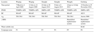
Datasets from six field campaigns were used in this paper. The six campaigns were conducted at four different measurement sites (Wangdu, Gucheng and Xianghe in Hebei province and Wuqing in Tianjin) of the North China Plain (NCP), the locations of these field campaign sites are displayed in Fig. S1 in the Supplement. Time periods and datasets used from these field campaigns are listed in Table 1. During these field campaigns, aerosol particles with aerodynamic diameters less than 10 µm were sampled (by passing through an impactor). The PNSDs in dry state, which range from 3 nm to 10 µm, were jointly measured by a Twin Differential Mobility Particle Sizer (TDMPS, Leibniz-Institute for Tropospheric Research, Germany; Birmili et al., 1999) or a scanning mobility particle size spectrometer (SMPS) and an Aerodynamic Particle Sizer (APS, TSI Inc., Model 3321) with a temporal resolution of 10 min. The mass concentrations of black carbon (BC) were measured using a Multi-Angle Absorption Photometer (MAAP Model 5012, Thermo, Inc., Waltham, MA USA) with a temporal resolution of 1 min during field campaigns of F1 to F5 and using an aethalometer (AE33) (Drinovec et al., 2015) during field campaign F6. The aerosol light scattering coefficients (σ_sp) at three wavelengths (450, 550, and 700 nm) were measured using a TSI 3563 nephelometer (Anderson and Ogren, 1998) during field campaigns of F1 to F5, and using an Aurora 3000 nephelometer (Müller et al., 2011) during field campaign F6.

Datasets of PNSD, BC and σ_sp from campaigns F2, F4 and F5 are referred to as D1. Measurements of PNSD and measurements from the humidified nephelometer system during campaign F6 (Gucheng campaign) are used to verify the proposed method of calculating the ambient ALWC. Details about the humidified nephelometer system during the Wangdu and Gucheng campaigns are introduced in detail in Kuang et al. (2017). During the Gucheng campaign, an In situ Gas and Aerosol Compositions Monitor (IGAC, Fortelice International Co.,Taiwan) was used for monitoring water-soluble ions (Na⁺, K⁺, Ca²⁺, Mg²⁺, ${\mathrm{NH}}_{\mathrm{4}}^{+}$, ${\mathrm{SO}}_{\mathrm{4}}^{\mathrm{2}-}$, ${\mathrm{NO}}_{\mathrm{3}}^{-}$, Cl⁻) of PM_2.5 and their precursor gases: NH₃, HCl, and HNO₃. The time resolution of IGAC measurements is 1 h. Ambient air was drawn into the IGAC system through a stainless-steel pipe wrapped with thermal insulation at a flow rate of 16.7 L min⁻¹. The ambient RH and temperature were observed using an automatic weather station with a time resolution of 1 min.

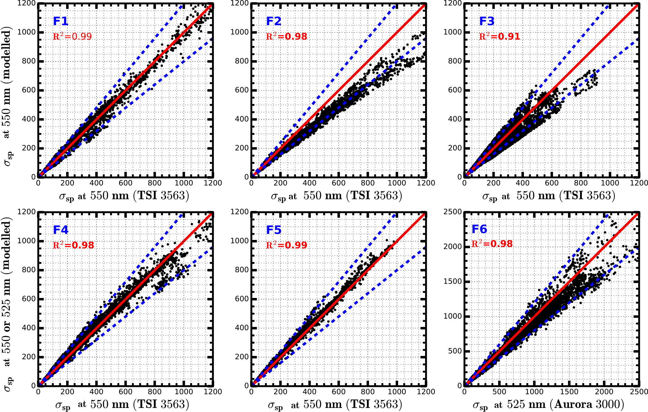
Figure 1 Comparisons between measured and calculated σ_sp (Mm⁻¹), solid red lines are 1 : 1 references lines. Dashed blue lines are 20 % relative difference lines. R² is square of correlation coefficient between measured and modelled σ_sp. Blue text in the upper left corners corresponds to field campaigns as listed in Table 1.

3 Methodology

3.1 Closure calculations

To ensure the datasets of σ_sp and PNSD used are of high quality, a closure study between measured σ_sp and that calculated based on measured PNSD and BC with Mie theory (Bohren and Huffman, 2008) is first performed. Measured σ_sp bears uncertainties introduced by angular truncation errors and nonideal light source. To achieve consistency between measured and modelled σ_sp, modelled σ_sp are calculated according to practical angular situations of the nephelometer (Anderson et al., 1996). During the σ_sp modelling process, BC was considered to be half externally and half core–shell mixed with other aerosol components. The mass size distribution of BC used in Ma et al. (2012), which was also observed in the NCP, was used in this research to account for the mass distributions of BC at different particle sizes. The applied refractive index and density of BC were 1.80−0.54i and 1.5 g cm⁻³ (Kuang et al., 2015). The refractive index of non-light-absorbing aerosol components (other than BC) was set to $\mathrm{1.53}-{\mathrm{10}}^{-\mathrm{7}}i$ (Wex et al., 2002). For the Mie theory calculation details please refer to Kuang et al. (2015).

The closure results between modelled σ_sp and σ_sp measured by TSI 3563 or Aurora 3000 using datasets observed during six field campaigns (Table 1) are depicted in Fig. 1. In general, for all six field campaigns, modelled σ_sp values correlate very well with measured σ_sp values. Considering the measured PNSD has an uncertainty of larger than 10 % (Wiedensohler et al., 2012), and the measured σ_sp has an uncertainty of about 9 % (Sherman et al., 2015), modelled σ_sp values agree well with measured σ_sp values in campaigns F1, F4, F5 and F6, with all points lying near the 1 : 1 line, and most points falling within the 20 % relative difference lines. For the closure results of field campaign F2, the modelled σ_sp values are systematically lower than measured σ_sp values. For the closure results of field campaign F3, most points also lie nearby 1 : 1 line, but points are relatively more dispersed.

3.2 Calculation of V_a (dry) based on measurements of the “dry” nephelometer

3.2.1 Theoretical relationship between V_a (dry) and σ_sp

Previous studies demonstrated that the σ_sp of aerosol particles is roughly proportional to V_a(dry) (Pinnick et al., 1980). Here, the quantitative relationship between V_a(dry) and σ_sp is analysed.

The σ_sp and V_a(dry) can be expressed as the following:

$$\begin{array}{}\text{(1)}& {\displaystyle }& {\displaystyle }{\mathit{\sigma }}_{\mathrm{sp}}=\int \mathit{\pi }{r}^{\mathrm{2}}{Q}_{\mathrm{sca}}\left(m,r\right)n\left(r\right)\mathrm{d}r,\text{(2)}& {\displaystyle }& {\displaystyle }{V}_{\mathrm{a}}\left(\mathrm{dry}\right)=\int {\displaystyle \frac{\mathrm{4}}{\mathrm{3}}}\mathit{\pi }{r}^{\mathrm{3}}n\left(r\right)\mathrm{d}r,\end{array}$$

where Q_sca(m,r) is scattering efficiency for a particle with refractive index m and particle radius r, while n(r) is the aerosol size distribution. As presented in Eqs. (1) and (2), relating V_a(dry) with σ_sp involves the complex relation between Q_sca(m,r) and particle diameter, which can be simulated using the Mie theory. According to the aerosol refractive index at visible spectral range, aerosol chemical components can be classified into two categories: the light absorbing component and the almost light non-absorbing components (inorganic salts and acids, and most of the organic compounds). Near the visible spectral range, the light absorbing component can be referred to as BC. BC particles are either externally or internally mixed with other aerosol components. In view of this, Q_sca at 550 nm, as a function of particle diameter for four types of aerosol particles, is simulated using Mie theory: almost non-absorbing aerosol particle, BC particle, BC particle core–shell mixed with non-absorbing components with the radii of the inner BC core being 50 and 70 nm, respectively. Same with those introduced in Sect. 2.2, the refractive indices of BC and light non-absorbing components used here are 1.80−0.54i and $\mathrm{1.53}-{\mathrm{10}}^{-\mathrm{7}}i$, respectively.

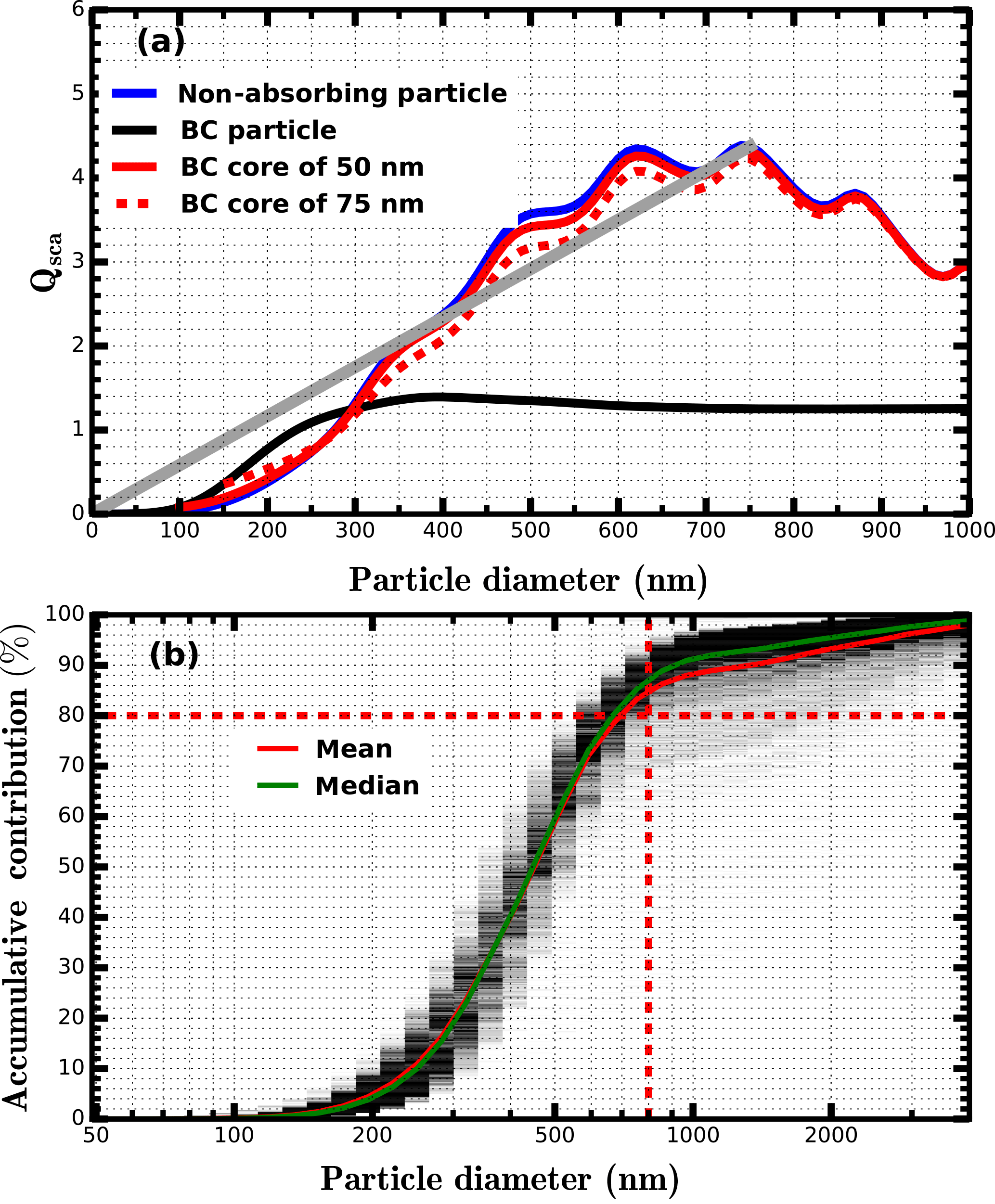
Figure 2 (a) Q_sca at 550 nm as a function of particle diameter for four types of aerosol particles: almost non-absorbing aerosol particle, BC particle, BC particle core–shell mixed with non-absorbing components and the radius of inner BC core are 50 and 70 nm. The grey line corresponds to the fitted linear line for the case of non-absorbing particle, when particle diameter is less than 750 nm. (b) Simulated size-resolved accumulative contribution to σ_sp at 550 nm for all PNSDs measured during the Wangdu campaign, the colour scales (from light grey to black) represent occurrences. The dashed dotted lines in panel (b) represent the position of 800 nm and 80 % contribution, respectively.

The simulated results are shown in Fig. 2a. Near the visible spectral range, most of the ambient aerosol components are almost non-absorbing, and their Q_sca varies more like the blue line shown in Fig. 2a. In that case, aerosol particles have diameters less than about 800 nm and Q_sca increases almost monotonously with particle diameter and can be approximately estimated as a linear function of diameter. Figure 2b shows the simulated size-resolved accumulative contribution to the scattering coefficient at 550 nm for all PNSDs measured during the Wangdu campaign. The results indicate that, for continental aerosol particles without influences of dust, in most cases, all particles with diameter less than about 800 nm contribute more than 80 % to the total σ_sp. Therefore, for Eq. (1) if we express Q_sca(m,r) as $Q_{\mathrm{sca}}(m,r)=k\cdot r$ then Eq. (1) can be expressed as the following:

$$\begin{array}{}\text{(3)}& {\mathit{\sigma }}_{\mathrm{sp}}=k\cdot \int \mathit{\pi }{r}^{\mathrm{3}}n\left(r\right)\mathrm{d}r.\end{array}$$

This explains why σ_sp(550 nm) is roughly proportional to V_a(dry). However, the value k varies greatly with particle diameter. The ratio σ_sp(550 nm) ∕ V_a(dry) (hereafter referred to as R_Vsp) is mostly affected by the PNSD, which determines the weight of influence different particle diameters have on R_Vsp. The discrepancy between the blue line and black line shown in Fig. 2a indicates that the fraction of externally mixed BC particles and their sizes has large impact on R_Vsp. The difference between the black line and the red line as well as the difference between the solid red line and the dashed red line shown in Fig. 2a indicate that the way and the amount of BC mixed with other components also exert significant influences on R_Vsp. In summary, the variation of R_Vsp is mainly determined by variations in PNSD, mass size distribution and the mixing state of BC. It is difficult to find a simple function describing the relationship between measured σ_sp and V_a(dry).

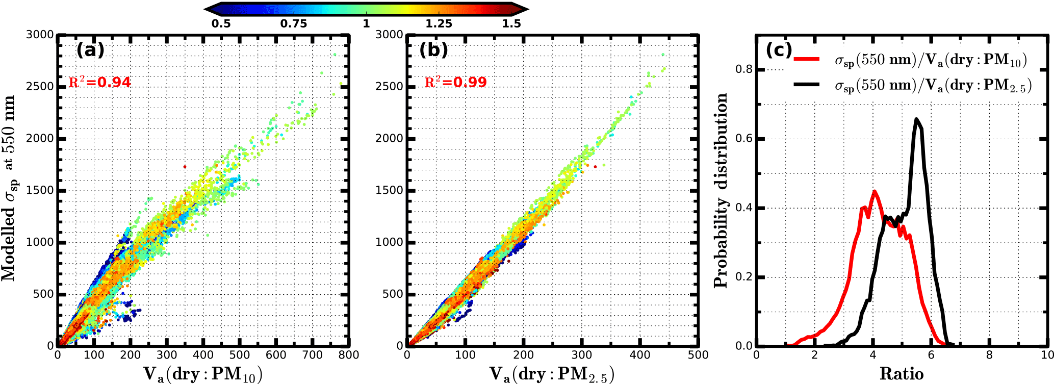
Figure 3 (a, b) Modelled σ_sp at 550 nm based on PNSD and BC vs. V_a(dry) of PM₁₀ or PM_2.5 calculated from measured PNSD. PNSD and BC datasets from six field campaigns listed in Table 1 are used. The unit of V_a(dry) is µm³ cm⁻³ and the unit of σ_sp is Mm⁻¹. Colours of scattered points in panels (a) and (b) represent corresponding values of the Ångström exponent. R² is the square of correlation coefficient. Panel (c) represents the probability distribution of the modelled ratio between σ_sp at 550 nm and V_a(dry) of PM₁₀ or PM_2.5.

Based on PNSD and BC datasets of field campaigns F1 to F6, the relationship between σ_sp at 550 nm and V_a(dry) of PM₁₀ or PM_2.5 are simulated using the Mie theory. The results are shown in Fig. 3. The results demonstrate that the σ_sp at 550 nm is highly correlated with the V_a(dry) of PM₁₀ and PM_2.5. The square of the correlation coefficient (r²) between σ_sp at 550 nm and V_a(dry) of PM₁₀ or PM_2.5 are 0.94 and 0.99, respectively. A roughly proportional relationship exists between V_a(dry) and σ_sp(550 nm), especially for V_a(dry) of PM_2.5. However, both R_Vsp of PM₁₀ and PM_2.5 vary significantly. R_Vsp of PM₁₀ mainly ranges from 2 to 6 cm³ (µm³ Mm)⁻¹, with an average of 4.2 cm³ (µm³ Mm)⁻¹. R_Vsp of PM_2.5 mainly ranges from 3 to 6.5 cm³ (µm³ Mm)⁻¹, with an average of 5.1 cm³ (µm³ Mm)⁻¹. Simulated size-resolved accumulative contributions to σ_sp at 550 nm for all PNSDs measured during campaigns F1 to F6 and corresponding size-resolved accumulative contributions to V_a(dry) of PM₁₀ are shown in Fig. S2. The results indicate that particles with diameter larger than 2.5 µm usually contribute negligibly to σ_sp at 550 nm but contribute about 20 % of the total PM₁₀ volume. Hence σ_sp at 550 nm is insensitive to changes in particles mass of diameters between 2.5 and 10 µm. This may partially explain why V_a(dry) of PM_2.5 correlates better with σ_sp at 550 nm than V_a(dry) of PM₁₀.

3.2.2 Machine learning

Based on analyses in Sect. 3.2.1, R_Vsp varies a lot with PNSD being the most dominant influencing factor. The “dry” nephelometer provides not only one single σ_sp at 550 nm, it measures six parameters including σ_sp and back scattering coefficients (σ_bsp) at three wavelengths (for TSI 3563: 450, 550 and 700 nm). The Ångström exponent calculated from spectral dependence of σ_sp provides information on the mean predominant aerosol size and is associated mostly with PNSD. The variation of the hemispheric backscattering fraction (HBF), which is the ratio between σ_bsp and σ_sp, is also essentially related to the PNSD. HBFs at three wavelengths (450, 550 and 700 nm) and the Ångström exponents calculated from σ_sp at different wavelengths (450–550, 550–700 and 450–700 nm) for typical non-absorbing aerosol particles with their diameters ranging from 100 nm to 3 µm are simulated using the Mie theory. The results are shown in Fig. 4a and b. HBF values at three different wavelengths and their differences are more sensitive to changes in PNSD of particle diameters less than about 400 nm. Ångström exponents calculated from σ_sp at different wavelengths almost decrease monotonously with particle diameter when particle diameter is less than about 1 µm; however, they differ distinctly when particle diameter is larger than 300 nm. These results indicate that HBFs at three wavelengths and Ångström exponents calculated from σ_sp at different wavelengths are sensitive to different diameter ranges of PNSD.

Thus, all six parameters measured by the “dry” nephelometer together can provide valuable information about variations in R_Vsp. However, no explicit formula exists between these six parameters and V_a(dry). How to use these six optical parameters is a problem; machine learning methods that can handle many input parameters are capable of learning from historical datasets and then make predictions, and strict relationships among variables are not required. Machine learning methods are powerful tools for tackling highly nonlinear problems and are widely used in different areas. In the light of this, predicting V_a(dry) based on six optical parameters measured by the “dry” nephelometer might be accomplished by using a machine learning method. In this study, random forest is chosen for this purpose.

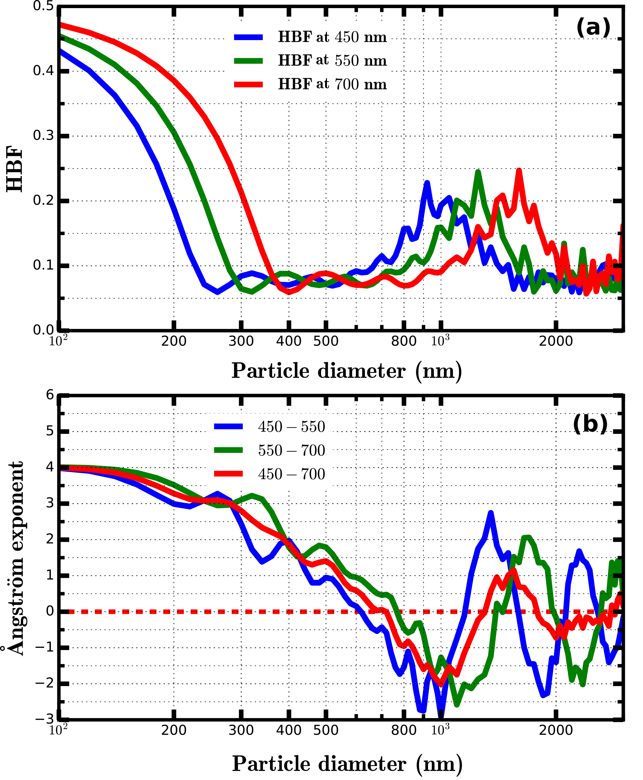
Figure 4 (a) Simulated HBF at three wavelengths as a function of particle diameter. (b) Simulated Ångström exponent values as a function of particle diameter.

Random forest is a machine learning technique that is widely used for classification and non-linear regression problems (Breiman, 2001). For non-linear regression cases, random forest model consists of an ensemble of binary regression decision tress. Each tree has a randomised training scheme, and an average over the whole ensemble of regression tree predictions is used for final prediction. In this study, the function RandomForestRegressor from the Python Scikit-Learn machine learning library (http://scikit-learn.org/stable/index.html, last access: 16 May 2018) is used. This model has several strengths. First, through averaging over an ensemble of decision trees there is a significantly lower risk of overfitting. Second, it involves fewer assumptions about the dependence between inputs and outputs when compared with traditional parametric regression models. The random forest model has two parameters: the number of input variables (N_in) and the number of trees grown (N_tree). In this study, N_in and N_tree are six and eight, respectively. The six input parameterises the three scattering coefficients, three backscattering coefficients.

The quality of input datasets is critical to the prediction accuracy of the machine learning method. As discussed in Sect. 3.1, modelled σ_sp during some field campaigns are not completely consistent with measured σ_sp, large bias might exist between them due to the measurement uncertainties of PNSD and σ_sp. To avoid the uncertainties in measurements of PNSD, aerosol optical properties are propagated in the training processes of the random forest model. In this study, both the required datasets of six optical parameters which corresponding to measurements of TSI 3563 and V_a(dry) for training the random forest model are calculated or simulated based on measurements of PNSD and BC from field campaigns F1 to F4 and F6. Datasets of PNSD and six optical parameters measured by the nephelometer during campaign F5 are used to verify the prediction ability of the trained random forest model. The performance of this random forest model on predicting both V_a(dry) of PM₁₀ and PM_2.5 are investigated. A schematic diagram of this method is shown in Fig. 5.

3.3 Connecting f(RH) to Vg(RH)

3.3.1 κ-Köhler theory

κ-Köhler theory is used to describe the hygroscopic growth of aerosol particles with different sizes, and the formula expression of κ-Köhler theory can be written as follows (Petters and Kreidenweis, 2007):

$$\begin{array}{}\text{(4)}& \mathrm{RH}={\displaystyle \frac{D^{\mathrm{3}}-D_{\mathrm{d}}^{\mathrm{3}}}{D^{\mathrm{3}}-D_{\mathrm{d}}^{\mathrm{3}}(\mathrm{1}-\mathit{\kappa })}}\cdot \exp \left({\displaystyle \frac{\mathrm{4}{\mathit{\sigma }}_{\mathrm{s}/\mathrm{a}}\cdot M_{\mathrm{water}}}{R\cdot T\cdot D_p\cdot g\cdot {\mathit{\rho }}_{\mathrm{w}}}}\right),\end{array}$$

where D is the diameter of the droplet, D_d is the dry diameter, σ_s∕a is the surface tension of solution/air interface, T is the temperature, M_water is the molecular weight of water, R is the universal gas constant, ρ_w is the density of water, and κ is the hygroscopicity parameter. By combining the Mie theory and the κ-Köhler theory, both f(RH) and Vg(RH) can be simulated. In the processes of calculations for modelling f(RH) and Vg(RH), the treatment of BC is same with those introduced in Sect. 2.2. As aerosol particle grows due to aerosol water uptake, the refractive index will change. In the Mie calculation, impacts of aerosol liquid water on the refractive index are considered based on volume mixing rule. The used refractive index of liquid water is $\mathrm{1.33}-{\mathrm{10}}^{-\mathrm{7}}i$ (Seinfeld and Pandis, 2006).

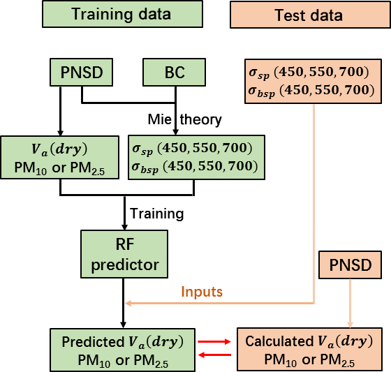
Figure 5 Schematic diagram of training the random forest (RF) model and verifying the performance of trained RF predictor. The trained datasets of PNSD and BC are from field campaigns F1 to F4 and F6, the test datasets of PNSD and optical parameters are from campaign F5 and σ_bsp is the backscattering coefficient.

3.3.2 Parameterization schemes for f(RH) and Vg(RH)

The f(RH) is defined as f(RH) = σ_sp(RH,550 nm) ∕ σ_sp(dry,550 nm), where σ_sp(RH,550 nm) and σ_sp(dry,550 nm) represents σ_sp at wavelength 550 nm under certain RH and dry conditions. Additionally, Vg(RH) is defined as Vg(RH) = V_a(RH) ∕ V_a(dry), where V_a(RH) represents total volume of aerosol particles under certain RH conditions.

A physically based single-parameter representation is proposed by Brock et al. (2016) to describe f(RH). The parameterization scheme is written as follows:

$$\begin{array}{}\text{(5)}& f\left(\mathrm{RH}\right)=\mathrm{1}+{\mathit{\kappa }}_{\mathrm{sca}}{\displaystyle \frac{\mathrm{RH}}{\mathrm{100}-\mathrm{RH}}},\end{array}$$

where κ_sca is the parameter which fits f(RH) best. Here, a brief introduction is given about the physical understanding of this parameterization scheme. For aerosol particles whose diameters larger than 100 nm, regardless of the Kelvin effect, the hygroscopic growth factor for an aerosol particle can be approximately expressed as g(RH) ≅ ${\left(\mathrm{1}+\mathit{\kappa }\frac{\mathrm{RH}}{\mathrm{100}-\mathrm{RH}}\right)}^{\frac{\mathrm{1}}{\mathrm{3}}}$ (Brock et al., 2016). Enhancement factor in volume can be expressed as the cube of g(RH). Aerosol particles larger than 100 nm contribute the most to σ_sp and V_a(dry) (as shown in Fig. S2). If a constant κ which represents the overall aerosol hygroscopicity of ambient aerosol particles is used as the κ of different particle sizes, then Vg(RH) can be approximately expressed as Vg(RH) = $\mathrm{1}+\mathit{\kappa }\frac{\mathrm{RH}}{\mathrm{100}-\mathrm{RH}}$. In addition, σ_sp is usually proportional to V_a(dry), which indicates that the relative change in σ_sp due to aerosol water uptake is roughly proportional to relative change in aerosol volume. Therefore, f(RH) might also be well described by using the formula form of Eq. (5). Previous studies have shown that this parameterization scheme can describe f(RH) well (Brock et al., 2016; Kuang et al., 2017).

During processes of measuring f(RH), the sample RH in the “dry” nephelometer (RH₀) is not zero. According to Eq. (5), the measured f(RH)${}_{\mathrm{measure}}=\frac{f\left(\mathrm{RH}\right)}{f\left({\mathrm{RH}}_{\mathrm{0}}\right)}$ should be fitted using the following formula:

$$\begin{array}{ll}{\displaystyle }& {\displaystyle }f{\left(\mathrm{RH}\right)}_{\mathrm{measure}}=\\ \text{(6)}& {\displaystyle }& {\displaystyle }\left(\mathrm{1}+{\mathit{\kappa }}_{\mathrm{sca}}{\displaystyle \frac{\mathrm{RH}}{\mathrm{100}-\mathrm{RH}}}\right)/\left(\mathrm{1}+{\mathit{\kappa }}_{\mathrm{sca}}{\displaystyle \frac{{\mathrm{RH}}_{\mathrm{0}}}{\mathrm{100}-{\mathrm{RH}}_{\mathrm{0}}}}\right).\end{array}$$

Based on this equation, κ_sca can be calculated from measured f(RH) directly. The typical value of RH₀ measured in the “dry” nephelometer during the Wangdu campaign is about 20 %. The importance of the RH₀ correction changes under different aerosol hygroscopicity and RH₀ conditions. The parameter κ_sca is fitted with and without consideration of RH₀ for f(RH) measurements during the Wangdu campaign, and the results are shown in Fig. S3. The results demonstrate that, overall, the κ_sca will be underestimated if the influence of RH₀ is not considered, and the larger the κ_sca, the more that the κ_sca will be underestimated.

In addition, based on discussions about the physical understanding of Eq. (5), the Vg(RH) should be well described by the following equation:

$$\begin{array}{}\text{(7)}& \mathrm{Vg}\left(\mathrm{RH}\right)=\mathrm{1}+{\mathit{\kappa }}_{\mathrm{Vf}}{\displaystyle \frac{\mathrm{RH}}{\mathrm{100}-\mathrm{RH}}},\end{array}$$

where κ_Vf is the parameter which fits Vg(RH) best. To validate this conclusion, a simulative experiment is conducted. In the simulative experiment, average PNSD in dry state and mass concentration of BC during the Haze in China (HaChi) campaign (Kuang et al., 2015) are used. During HaChi campaign, size-resolved κ distributions are derived from measured size-segregated chemical compositions (Liu et al., 2014) and their average is used in this experiment to account the size dependence of aerosol hygroscopicity. Modelled results of f(RH) and Vg(RH) are shown in Fig. S4. Results demonstrate that modelled f(RH) and Vg(RH) can be well parameterized using the formula form of Eqs. (5) and (7). Fitted values of κ_sca and κ_Vf are 0.227 and 0.285, respectively. This result indicates that if linkage between κ_sca and κ_Vf is established, measurements of f(RH) can be directly related to Vg(RH).

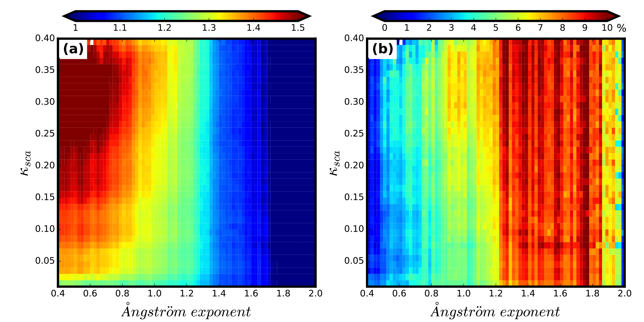
Figure 6 (a) Colours represent R_Vf values and the colour bar is shown on the top of this figure, x axis represents the Ångström exponent and y axis represents κ_sca. (b) Meanings of x axis and y axis are same as those in panel (a). However, colour represents the percentile value of the standard deviation of R_Vf values within each grid divided by their average.

3.3.3 Bridge the gap between f(RH) and Vg(RH)

Many factors have significant influences on the relationships between f(RH) and Vg(RH), including PNSD, BC mixing state and the size-resolved aerosol hygroscopicity. To gain insights into the relationships between κ_sca and κ_Vf, a simulative experiment using Mie theory and κ-Köhler theory is designed. In this experiment, all PNSDs at dry state along with mass concentrations of BC from D1 are used, characteristics of these PNSDs can be found in Kuang et al. (2017). As to size-resolved aerosol hygroscopicity, a number of size-resolved κ distributions were derived from measured size-segregated chemical compositions during HaChi campaign (Liu et al., 2014). Results from other research also show similar size dependence of aerosol hygroscopicity (Meng et al., 2014). In view of this, the shape of the average size-resolved κ distribution during HaChi campaign (black line shown in Fig. S5) is used in the designed experiment. Other than the shape of size-resolved κ distribution, the overall aerosol hygroscopicity, which determines the magnitude of f(RH), also has a large impact on the relationship between κ_sca and κ_Vf. In view of this, ratios ranging from 0.05 to 2, with an interval of 0.05, are multiplied with the average size-resolved κ distribution (the black line shown in Fig. S5) to produce a number of size-resolved κ distributions which represent aerosol particles from nearly hydrophobic to highly hygroscopic. During simulating processes, each PNSD is modelled with all produced size-resolved κ distributions. In the following, the ratio κ_Vf∕κ_sca, termed as R_Vf, is used to indicate the relationship between κ_sca and κ_Vf.

Considering that values of the Ångström exponent contain information about PNSD (Kuang et al., 2017) and values of κ_sca represent overall hygroscopicity of ambient aerosol particles, and that both of these parameters can be directly calculated from measurements of a three-wavelength humidified nephelometer system (Kuang et al., 2017), simulated R_Vf values are spread into a two-dimensional gridded plot. The first dimension is the Ångström exponent with an interval of 0.02 and the second dimension is κ_sca with an interval of 0.01. Average R_Vf value within each grid is represented by colour and shown in Fig. 6a. Values of the Ångström exponent corresponding to used PNSDs are calculated from simultaneously measured σ_sp values at 450 and 550 nm from the TSI 3563 nephelometer. Results shown in Fig. 6a exhibit that both PNSD and overall aerosol hygroscopicity have significant influences on R_Vf. Simulated values of R_Vf range from 0.8 to 1.7, with an average of 1.2. Overall, the R_Vf value is lower when the value of the Ångström exponent is larger. The percentile value of standard deviation of R_Vf values within each grid, divided by its average, is shown in Fig. 6b. In most cases, these percentile values are less than 10 % (about 90 %) which demonstrates that R_Vf varies little within each grid shown in Fig. 6a. Figure 6 shows the influence of aerosol size and chemistry on R_Vf. For an Ångström exponent less than ∼ 1.1, R_Vf varies strongly with κ_sca. However, for an Ångström exponent values greater than ∼ 1.1, the R_Vf relative standard deviation exhibits a higher variability with the Ångström exponent, thus showing the sensitivity of R_Vf to changes in aerosol size for small particles. In general, results shown in Fig. 6 imply that results of Fig. 6a can serve as a lookup table to estimate R_Vf and thereby κ_Vf, such that these values can be directly predicted from measurements of a three-wavelength humidified nephelometer system.

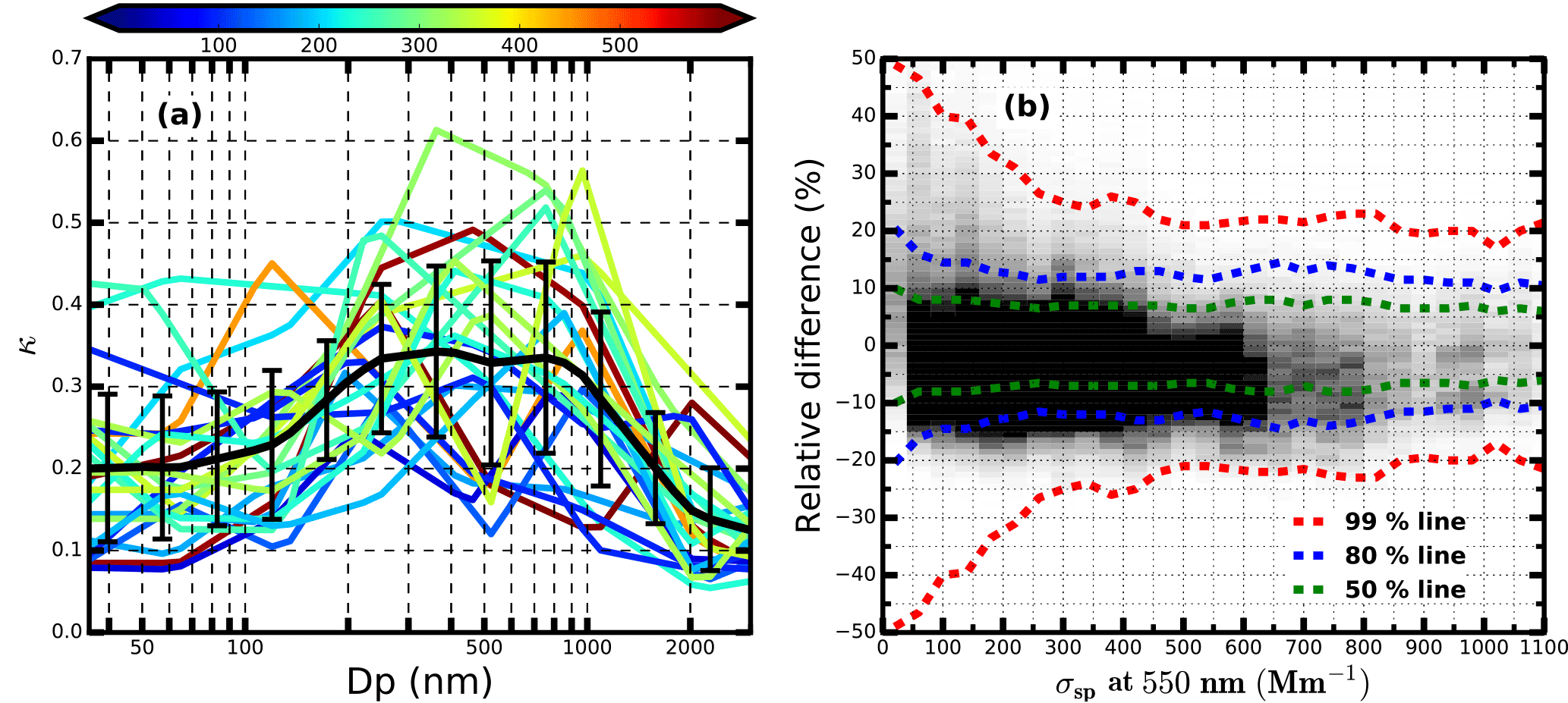
Figure 7 (a) All size-resolved κ distributions, which are derived from measured size-segregated chemical compositions during HaChi campaign, colours represent corresponding values of average σ_sp at 550 nm (Mm⁻¹), the black solid line is the average size-resolved κ distribution and error bars are standard deviations; (b) the grey colours represent the distribution of relative differences between modelled and estimated R_Vf values, darker grids have higher frequency and dashed lines with the same colour mean that corresponding percentile of points locate between the two lines.

For the lookup table shown in Fig. 6a, a fixed size-resolved κ distribution is used, which might not be able to capture variations of R_Vf induced by different types of size-resolved κ distributions under different PNSD conditions. A simulative experiment is conducted to investigate the performance of this lookup table. In this experiment, the following datasets are used: PNSDs and mass concentrations of BC from D1 (the number of used PNSD is 11996), and size-resolved κ distributions from HaChi campaign (Liu et al., 2014), which are presented in Fig. 7a (the number is 23). Results shown in Fig. 7a imply that the shape of size-resolved κ distribution is highly variable, yet has no apparent correlation with aerosol loading. During the simulating processes for each PNSD, it is used to simulate R_Vf values corresponding to all used size-resolved κ distributions; therefore, 275 908 R_Vf values are modelled. Also, modelled values of κ_sca and corresponding values of the modelled Ångström exponent are used together to estimate R_Vf values using the lookup table shown in Fig. 7a. Results of relative differences between estimated and modelled R_Vf, values under different pollution conditions are shown in Fig. 7b. Overall, 88 % of points have absolute relative differences less than 15 % and 68 % of points have absolute relative differences less than 10 %. This lookup table performs better when the air is relatively polluted.

3.4 Calculation of ambient ALWC

According to the equation Vg(RH) = $\mathrm{1}+{\mathit{\kappa }}_{\mathrm{Vf}}\frac{\mathrm{RH}}{\mathrm{100}-\mathrm{RH}}$, ALWC refers to volume concentrations of aerosol liquid water at different RH points and can be expressed as the following:

$$\begin{array}{ll}{\displaystyle }\mathrm{ALWC}& {\displaystyle }=V_{\mathrm{a}}\left(\mathrm{dry}\right)\times (\mathrm{Vg}\left(\mathrm{RH}\right)-\mathrm{1})\\ \text{(8)}& {\displaystyle }& {\displaystyle }=V_{\mathrm{a}}\left(\mathrm{dry}\right)\cdot {\mathit{\kappa }}_{\mathrm{sca}}\cdot R_{\mathrm{Vf}}\cdot {\displaystyle \frac{\mathrm{RH}}{\mathrm{100}-\mathrm{RH}}}.\end{array}$$

According to discussions of Sect. 3.2, V_a(dry) can be predicted based only on measurements from the “dry” nephelometer by using a random forest model. The training of the random forest model requires only regional historical datasets of simultaneously measured PNSD and BC. The κ_sca is directly fitted from f(RH) measurements. The R_Vf can be estimated using the lookup table introduced in Sect. 3.3. Thus, based only on measurements from a three-wavelength humidified nephelometer system, ALWCs of ambient aerosol particles at different RH points can be estimated. If both measurements from the humidified nephelometer system and ambient RH are available, ambient ALWC can be calculated. The flowchart of calculating ambient ALWC based on measurements of the humidified nephelometer system is shown in Fig. 8. The nephelometer used, corresponding to this flowchart, should be TSI 3563. If nephelometer of the used humidified nephelometer system is Aurora 3000, wavelengths in this flowchart will change but other steps are totally the same.

4 Results and discussion

4.1 Validation of the random forest model for predicting V_a(dry) based on measurements of the “dry” nephelometer

The machine learning method, random forest model, is proposed to predict V_a(dry) based only on σ_sp and σ_bsp at three wavelengths measured by the “dry” nephelometer. Datasets of PNSD and BC from field campaigns F1 to F4 and F6 are used to train the random forest model. Datasets of PNSD and optical parameters measured by the “dry” nephelometer from field campaign F5 are used to verify the trained random forest model. The schematic diagram of this method is shown in Fig. 5. The comparison results between calculated and predicted V_a(dry) of PM₁₀ and PM_2.5 are shown in Fig. 9. The square of correlation coefficient between predicted and calculated V_a(dry) of PM₁₀ is 0.96, and almost all points lie between or near 20 % relative difference lines. The square of correlation coefficient between predicted and calculated V_a(dry) of PM_2.5 is 0.997, and almost all points lie between or near 10 % relative difference lines. The standard deviations of relative differences between predicted and calculated V_a(dry) of PM₁₀ and PM_2.5 are 10 and 4 %, respectively. These results indicate that V_a(dry) of PM_2.5 can be well predicted by using the machine learning method. While V_a(dry) of PM₁₀ predicted by using the machine learning method has a relatively larger bias.

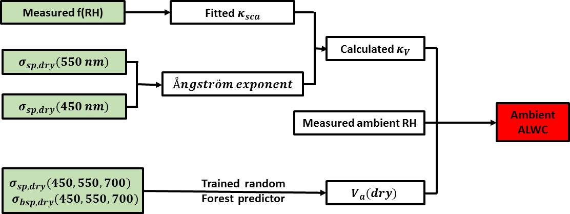
Figure 8 The flowchart of calculating ambient aerosol liquid water contents based on measurements of a three-wavelength humidified nephelometer system.

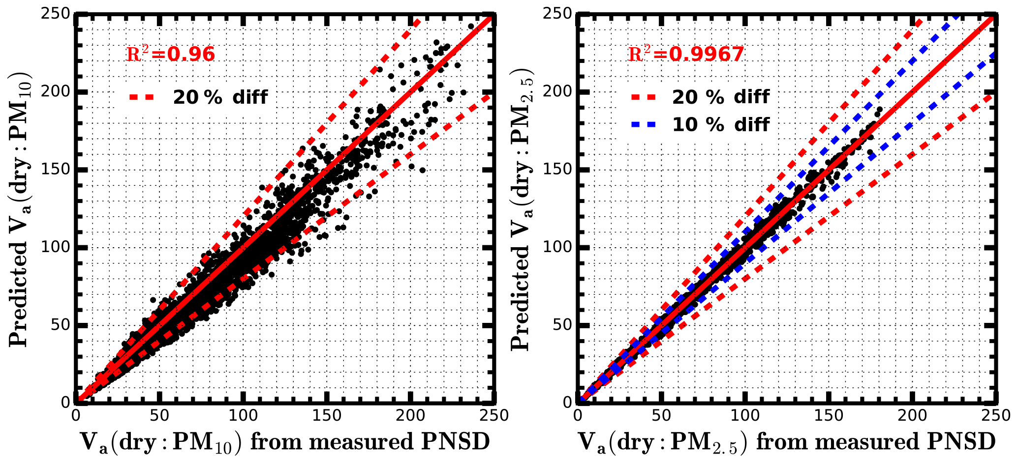
Figure 9 The comparison between V_a(dry) (µm³ cm⁻³) of PM₁₀ or PM_2.5, calculated from measured PNSD and V_a(dry) of PM₁₀ or PM_2.5, which are predicted based on six optical parameters measured by the “dry” nephelometer, by using the random forest model. R² is the square of correlation coefficient. The solid red line is the 1 : 1 line, dashed red lines and dashed blue lines represent 20 and 10 % relative difference lines.

Machine learning methods do not explicitly express relationships between many variables; however, they learn and implicitly construct complex relationships among variables from historical datasets. Many different and comprehensive machine learning methods are developed for diverse applications and can be directly used as a tool for solving a lot of nonlinear problems which may not be mathematically well understood. We suggest using a machine learning method for estimating V_a(dry) based on measurements of the “dry” nephelometer. The way of estimating V_a(dry) with machine learning method might be applicable for different regions around the world if used estimators are trained with corresponding regional historical datasets.

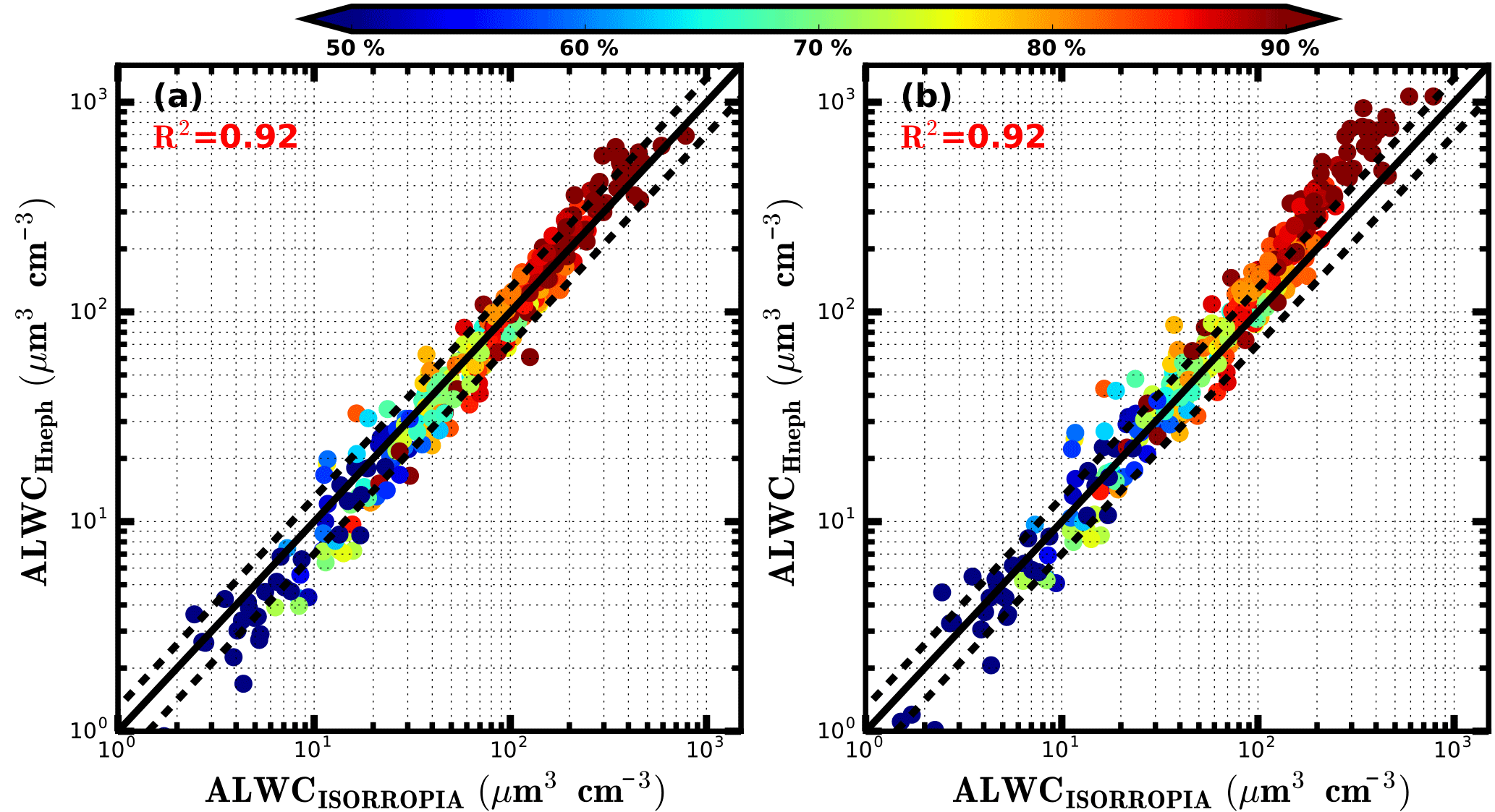
Figure 10 The comparison between ALWC calculated from ISORROPIA thermodynamic model (ALWC_ISORROPIA) and ALWC calculated from measurements of the humidified nephelometer system (ALWC_Hneph). The black solid line is the 1 : 1 line and the two dashed black lines are 30 % relative difference lines. R² is the square of correlation coefficient. Colours of scatter points represent ambient RH. (a) ALWC_Hneph is calculated using the method proposed in this research. (b) ALWC_Hneph is calculated by assuming Vg(RH) = f(RH)^1.5 (Guo et al., 2015).

4.2 Comparison between ambient ALWC calculated from ISORROPIA and measurements of the humidified nephelometer system

So far, widely used tools for prediction of ambient ALWC are thermodynamic models. ISORROPIA-II thermodynamic model (http://nenes.eas.gatech.edu/ISORROPIA/index_old.html, last access: 16 May 2018) is a famous one and is widely used in research for predicting pH and ALWC of ambient aerosol particles (Guo et al., 2015; Cheng et al., 2016; Liu et al., 2017; Fountoukis and Nenes, 2007). Water-soluble ions and gaseous precursors are required as inputs of thermodynamic model. During the Gucheng campaign, measurements from both the humidified nephelometer system and IGAC are available. Thus, the ambient ALWC can be calculated through two independent methods: thermodynamic model based on IGAC measurements and the method proposed in Sect. 3.4, which is based on measurements of the humidified nephelometer system. In this study, the forward mode in ISORROPIA-II is used and water-soluble ions in PM_2.5 and gaseous precursors (NH₃, HNO₃, HCl) measured by the IGAC instrument along with simultaneously measured RH and T are used as inputs. The aerosol water associated with organic matter is not considered in the method of ISORROPIA model, due to the lack of measurements of organic aerosol mass. However, results from previous studies indicate that organic matter induced particle water only account for about 5 % of total ALWC (Liu et al., 2017). For the ALWC calculated from the humidified nephelometer system, the needed V_a(dry) of PM_2.5 in Eq. (7) is calculated from simultaneously measured PNSD.

The comparison results between ambient ALWC calculated from these two independent methods are shown in Fig. 10a. The square of correlation coefficient between them is 0.92, most of the points lie within or nearby 30 % relative difference lines. The slope is 1.14, and the intercept is −8.6 µm³ cm⁻³. When ambient RH is higher than 80 %, the ambient ALWCs calculated from measurements of the humidified nephelometer system are higher relative to those calculated based on ISORROPIA-II. When ambient RH is lower than 60 %, the ambient ALWCs calculated from measurements of the humidified nephelometer system are lower relative to those calculated based on ISORROPIA-II. Overall, a good agreement is achieved between ambient ALWC calculated from measurements of the humidified nephelometer system and ISORROPIA thermodynamic model.

Figure 11 Volume fractions of water in total volume of ambient aerosols during the Wangdu (WD) and Gucheng (GC) campaigns. X axis represents measured ambient RH. The y axis represents volume fractions of water. Colours of scatter points represent corresponding κ_Vf. Black solid lines in panels (a) and (b) show the average volume fractions of water under different ambient RH conditions.

Guo et al. (2015) conducted the comparison between ambient ALWC calculated from ISORROPIA model and ambient ALWC calculated from measurements of the humidified nephelometer system by assuming Vg(RH) = f(RH)^1.5. Thus, the comparison results between ambient ALWC calculated based on ISORROPIA and ambient ALWC calculated by assuming Vg(RH) = f(RH)^1.5 are also shown in Fig. 10b. The square of the correlation coefficient between them is also 0.92. However, the slope and intercept are 1.7 and −21 µm³ cm⁻³, respectively. When the ambient RH is higher than about 80 %, calculated ambient ALWC will be significantly overestimated if it is assumed that Vg(RH) = f(RH)^1.5. This method assumes that average scattering efficiency of aerosol particles at dry state and different RH conditions are the same. When ambient RH is high, the particle diameters changes a lot. As the results shown in Fig. S6, for non-absorbing particle, when diameter of aerosol particle in dry state is less than 500 nm, the aerosol scattering efficiency increase almost monotonously with increasing RH especially when RH is higher than 80 %. Therefore, it is not suitable to assume that average scattering efficiency of aerosol particles at dry state and different RH conditions are the same.

4.3 Volume fractions of ALWC in total ambient aerosol volume

During the Wangdu campaign, κ_sca ranged from 0.05 to 0.3 with an average of 0.19. Estimated values of R_Vf ranges from 0.86 to 1.47, with an average of 1.15. Estimated values of κ_Vf ranges from 0.05 to 0.35, with an average of 0.22. The calculated volume fractions of water in total volume of ambient aerosols during the Wangdu campaign are shown in Fig. 11a. The results indicate that during the Wangdu campaign, when ambient RH is higher than 70 %, the κ_Vf values are relatively higher. The volume fractions of water are always higher than 50 % when ambient RH is higher than 80 %.

During the Gucheng campaign, κ_sca ranges from 0.008 to 0.22 with an average of 0.1, κ_Vf ranges from 0.01 to 0.21 with an average of 0.12. The aerosol hygroscopicity during the Gucheng campaign is much lower than aerosol hygroscopicity during the Wangdu campaign. The calculated volume fractions of water in total volume of ambient aerosols during the Gucheng campaign are shown in Fig. 11b. During the Gucheng campaign, the maximum volume fraction of water in ambient aerosol is 42 % when ambient RH is at 80 %. On average, when ambient RH is higher than 90 %, the volume fraction of water in ambient aerosols reaches higher than 50 %.

4.4 Discussions about the applicability of the proposed method

The method proposed in this research is based on datasets of PNSD, σ_sp and size-resolved κ distribution, which are measured on the NCP without influences of dust events and sea salt. Caution should be exercised if using the proposed method to estimate the ALWC when the air mass is significantly influenced by sea salt or dust. The way of estimating V_a(dry) with machine learning method might be applicable for different regions around the world. However, the used predictor from machine learning should be trained with corresponding regional historical datasets of PNSD and BC. The way of connecting f(RH) to Vg(RH) might also be applicable for other continental regions. Still, we suggest that the used lookup table is simulated from regional historical datasets.

Note that the humidified nephelometer usually operates with RH less than 95 %. However, aerosol water increase dramatically with increasing RH when RH is greater than 95 %. Such high RH conditions can occur during the haze events. This may limit the usage of the proposed method when ambient RH is extremely high. As discussed in Sect. 3.3, the proposed way of connecting f(RH) and Vg(RH) is based on the κ-Köhler theory. If κ does not change with RH, the proposed method should be applicable when RH is higher than 95 %, even if the measurements of humidified nephelometer system are conducted when RH is less than 95 %. Many studies have done research about the change of κ with the changing RH (Rastak et al., 2017; Renbaum-Wolff et al., 2016), their results demonstrate that the κ changes with increasing RH. However, few studies have investigated the variation of κ of ambient aerosol particles with changing RH when RH is less than 100 %. Liu et al. (2011) have measured κ of ambient aerosol particles at different RHs (90, 95 and 98.5 %) on the NCP. Their results demonstrated that κ at different RHs differs little for ambient aerosol particles with different diameters. Results of Kuang et al. (2017) indicated that κ values retrieved from f(RH) measurements agree well with κ values at RH of 98 % of aerosol particles with diameter of 250 nm. In this respect, the proposed method might be applicable even when ambient RH is extremely high for ambient aerosol particles on the NCP. Moreover, for calculating the ambient ALWC, the measured ambient RH is required. If the ambient RH is higher than 95 %, the measured ambient RH with current techniques is highly uncertain. Given this, cautions should be exercised if the ambient ALWC is calculated when the ambient RH is higher than 95 %.

5 Conclusions

In this paper, a novel method is proposed to calculate ALWC based on measurements of a three-wavelength humidified nephelometer system. Two critical relationships are required in this method. One is the relationship between V_a(dry) and measurements of the “dry” nephelometer. Another one is the relationship between Vg(RH) and f(RH). The ALWC can be calculated from the estimated V_a(dry) and Vg(RH).

Previous studies have shown that an approximate proportional relationship exists between V_a(dry) and corresponding σ_sp, especially for fine particles (particle diameter less than 1 µm). However, PNSD and other factors still have significant influences on this proportional relationship. It is difficult to directly estimate V_a(dry) from measured σ_sp. In this paper, a random forest predictor from machine learning procedure is used to estimate V_a(dry) based on measurements of a three-wavelength nephelometer. This random forest predictor is trained based on historical datasets of PNSD and BC from several field campaigns conducted on the NCP. This method is then validated using measurements from the Wangdu campaign. The square of correlation coefficient between measured and estimated V_a(dry) of PM₁₀ and PM_2.5 are 0.96 and 0.997, respectively.

The relationship between Vg(RH) and f(RH) is investigated in Sect. 3 by conducting a simulative experiment. It is found that the complicated relationship between Vg(RH) and f(RH) can be disentangled by using a lookup table, and parameters required in the lookup table can be directly calculated from measurements of a three-wavelength humidified nephelometer system. Given that the V_a(dry) can be estimated from a three-wavelength “dry” nephelometer, the ambient ALWC can be estimated from measurements of a three-wavelength humidified nephelometer system in conjunction with measured ambient RH. We have conducted the comparison between ambient ALWC calculated from ISORROPIA and ambient ALWC calculated from measurements of the humidified nephelometer system. The square of correlation coefficient between them is 0.92, and most of the points lie within or nearby 30 % relative difference lines. The slope and intercept are 1.14 and −8.6 µm³ cm⁻³, respectively. Overall, a good agreement is achieved between ambient ALWC calculated from measurements of the humidified nephelometer system and ISORROPIA thermodynamic model.

Results introduced in this research have bridged the gap between f(RH) and Vg(RH). The advantage of using measurements of a humidified nephelometer system to estimate ALWC is that this technique has a fast response time and can provide continuous measurements of the changing ambient conditions. The new method proposed in this research will facilitate the real-time monitoring of the ambient ALWC and further our understanding of roles of ALWC in atmospheric chemistry, secondary aerosol formation and climate change.

Appendix A: Abbreviations

RH	relative humidity
PM2.5	particulate matter with aerodynamic diameter of less than 2.5 µm
PM10	particulate matter with aerodynamic diameter of less than 10 µm
f(RH)	aerosol light scattering enhancement factor at 550 nm
ALWC	aerosol liquid water content: volume concentrations of water in ambient aerosols
Va(dry)	total volume of ambient aerosol particles in dry state
Vg(RH)	aerosol volume enhancement factor due to water uptake
NCP	North China Plain
HTDMA	humidified tandem differential mobility analyser system
PNSD	particle number size distribution
BC	black carbon
g(RH)	hygroscopic growth factor
APS	Aerodynamic Particle Sizer
SMPS	scanning mobility particle size spectrometer
σsp	aerosol light scattering coefficient
σbsp	aerosol back scattering coefficient
σext	aerosol extinction coefficient
RVsp	σsp(550 nm) ∕ Va(dry)
F1 to F6	referred as to five field campaigns listed in Table 1
D1	PNSD, BC and nephelometer measurements from F2, F4 and F5