Evaluating tropospheric humidity from GPS radio occultation, radiosonde, and AIRS from high-resolution time series

While water vapor is the most important tropospheric greenhouse gas, it is also highly variable in both space and time, and water vapor concentrations range over 3 orders of magnitude in the troposphere. These properties challenge all observing systems to accurately measure and resolve the vertical structure and variability of tropospheric humidity. In this study we characterize the humidity measurements of various observing techniques, including four separate Global Positioning System (GPS) radio occultation (RO) humidity retrievals (University Corporation for Atmospheric Research (UCAR) direct, UCAR one-dimensional variational retrieval (1D-Var), Wegener Center for Climate and Global Change (WEGC) 1D-Var, Jet Propulsion Laboratory (JPL) direct), radiosonde, and Atmospheric Infrared Sounder (AIRS) data. Furthermore, we evaluate how well the ERA-Interim reanalysis and NCEP Global Forecast System (GFS) model perform in analyzing water vapor at different levels. To investigate detailed vertical structure, we analyzed time–height cross sections over four radiosonde stations in the tropical and subtropical western Pacific for the year 2007. We found that the accuracy of RO humidity is comparable to or better than both radiosonde and AIRS humidity over 800 to 400 hPa, as well as below 800 hPa if super-refraction is absent. The various RO retrievals of specific humidity agree within 20 % in the 1000–400 hPa layer, and differences are most pronounced above 600 hPa.

1 Introduction

Tropospheric humidity is one of the key parameters driving weather and climate, and it plays an important role in the development of many extreme events. To accurately model current and future climate, it is crucial to understand the distribution, transport, and vertical structure of tropospheric water vapor. However, measuring water vapor accurately is a great challenge, as it is highly variable on both spatial and temporal scales, and its tropospheric concentration varies over 3 orders of magnitude between the tropical planetary boundary layer (PBL) and the tropopause. At present, no single observing system can provide accurate tropospheric humidity data on a global scale with high vertical resolution.

Passive (microwave and infrared) nadir-sounding systems provide data globally, but with relatively low vertical resolution. Weighting functions are used to quantify vertically resolved humidity information, and these vertical scales are large (2 to 3 km) compared to the variability of water vapor in the vertical. Furthermore, infrared-based systems cannot provide data within or below clouds.

Radiosonde (RS) balloon measurements are launched globally, although with sparse coverage in many areas, such as over oceans or in the Southern Hemisphere. They can have a high vertical resolution, but data quality varies strongly depending on the sensor type (Miloshevich et al., 2006; Ho et al., 2010). Operational weather forecasting still benefits greatly from RS measurements, but the current global RS network is neither designed nor suitable for detecting and monitoring climate change. First, many different sensor types are used globally, each with their unique known and unknown biases. Second, sensor types at different locations change over time, and these changes have been poorly documented in the past, which can lead to artificial trends or jumps in the station's record (Dai et al., 2011). The GCOS (Global Climate Observing System) Reference Upper-Air Network (GRUAN) aims to address this issue by providing long-term high-quality vertical profiles of selected essential climate variables, including an estimate of the measurement uncertainty (Bodeker et al., 2016). GRUAN will play an important role for calibrating data from other global networks; however, at this point in time certified data are available at only a few locations with a relatively short time range (less than 4 years).

Research aircraft can provide high-quality, high-resolution profiles, but these missions are infrequent and cannot provide a complete global picture continuously over time by themselves. They are, however, important to evaluate measurements from other observing systems or models (Rieckh et al., 2017).

The Global Positioning System (GPS) radio occultation (RO) technique provides near-vertical profiles of refractivity with high vertical resolution and high accuracy and precision. Other features of the RO technique are global coverage, all-weather capability, and SI traceability. Profiles penetrating down into the lower troposphere became available with open-loop tracking (Sokolovskiy et al., 2006). Since refractivity depends on temperature and water vapor pressure, tropospheric specific humidity can be derived from refractivity via a so-called direct retrieval (using ancillary temperature information) or a one-dimensional variational retrieval (1D-Var), which finds the optimal solution for water vapor pressure, temperature, and refractivity, taking their prescribed errors into account. Thus the RO water vapor retrievals and their quality vary depending on the a priori (and the accuracy of the prescribed data) and inversion method used. Several RO processing centers currently provide RO water vapor profile retrievals: University Corporation for Atmospheric Research (UCAR), Jet Propulsion Laboratory (JPL), Danish Meteorological Institute (DMI), and Wegener Center for Climate and Global Change (WEGC).

The above observing techniques have been used to investigate the global humidity distribution, trends, and radiative impact. RO, despite being a relatively young observing technique, has shown the potential to provide data of climate benchmark quality for refractivity and temperature between about 8 and 25 km (Ho et al., 2009, 2012; Steiner et al., 2013). The quality of RO humidity is subject to research since ancillary data are required to retrieve humidity from refractivity. Kursinski et al. (1995) provided a first estimate for water vapor accuracy of less than 5 % for individual profiles in the boundary layer and 20 % up to about 7 km. Chou et al. (2009) found humidity differences smaller than 40 % below 7 km for individual profile comparisons between dropsondes and RO. For observations near strong typhoons, they found differences up to 100 % in the mid- and upper troposphere. Regarding global specific-humidity distributions, Chou et al. (2009) found good agreement within 15 % between RO and Atmospheric Infrared Sounder (AIRS) but significant discrepancy between NCEP/NCAR reanalysis and RO humidity. Ho et al. (2010) showed that UCAR COSMIC (Constellation Observing System for Meteorology, Ionosphere, and Climate) water vapor profiles agree well with those of European Centre for Medium-range Weather Forecasts (ECMWF) analysis over different regions, demonstrating the quality of the RO humidity data. Furthermore, they used RS and RO co-located data to identify biases of various RS types. Wang et al. (2013) also used UCAR COSMIC water vapor products and global RS data with very strict co-location criteria (1 h, 100 km) to verify the quality of UCAR RO humidity and found a mean specific-humidity bias of −0.012 g kg⁻¹, with a standard deviation of 0.666 g kg⁻¹ over the 925–200 hPa layer. Ladstädter et al. (2015) compared WEGC RO profiles from multiple missions to a 5-year record of GRUAN RS profiles (both of which have the potential to serve as reference observations in the GCOS) and to a standard 11-year record of RS profiles (Vaisala RS90/92). Vaisala RS90/92 shows a dry bias of 40 % in the troposphere compared to RO, whereas GRUAN, with an elaborate humidity bias correction scheme, agrees within 5 % with RO below 300 hPa. Ladstädter et al. (2015) state that the good agreement of the RO and GRUAN RS data sets strongly encourages further development and advancement of both systems for the benefit of future climate monitoring and research. Vergados et al. (2015) compared relative humidity (RH) of JPL RO, ECMWF ERA-Interim reanalysis, and Modern-Era Retrospective analysis for Research and Applications (MERRA) in the tropics and showed that, from a climatological standpoint, MERRA and JPL RO are in agreement, whereas the ECMWF reanalysis is drier. Vergados et al. (2018) compared JPL and UCAR RO humidity data sets to MERRA, ERA-Interim, and AIRS from 2007 to 2015 for the $\pm \mathrm{40}{}^{\circ }$ latitude range between 700 and 400 hPa. They found that both RO humidity retrievals agree well with MERRA and ERA-Interim, but the JPL retrieval is overall moister than all other data sets, while both the UCAR retrieval and AIRS are overall drier than all other data sets.

All of the above work considered differences averaged over large geographical regions and long time periods (a month or longer). While useful for climate and error estimations, these averages obscure variability that takes place on smaller temporal and spatial scales. Case studies fill this gap, but they often focus on a single particular event that occurs over only a few days.

In this study we focus on the water vapor variability in both a temporal and spatial sense by comparing data from multiple observing techniques (RO, RS, AIRS) and model (re)analyses (ERA-Interim, Global Forecast System (GFS)) at particular locations in the tropics and sub-tropics over an entire year. We chose the year 2007, when the maximum number of COSMIC RO profiles was available (COSMIC was launched in 2006; Anthes et al., 2008). We compare each of these individual data sets with co-located ERA-Interim humidity results for (a) the surface to the upper troposphere, (b) four locations, (c) four seasons, and (d) during typhoon passages. We quantify the structural uncertainty of RO-derived humidity profiles in the troposphere, which results from different inversion implementations and a priori. To understand how the RO humidity data sets are different from other humidity products, we collected RS–ERA pairs, AIRS–ERA pairs, and GFS–ERA pairs near the four RS stations. Although these data pairs may not sample the same local times, the errors due to local time sampling differences are probably small over these oceanic regions.

As humidity varies strongly in time and space, this study allows us to show in detail how humidity conditions change over time, both daily and seasonally, and how atmospheric conditions affect the ability of these data sets to provide accurate and precise humidity information. We can identify high-frequency variability and patterns at selected locations that would be obscured if only statistical parameters were analyzed.

We focus on several challenging locations in the tropics and sub-tropics where water vapor is highly variable. We show the entire 1000–400 hPa range to show how data quality for different observing and modeling systems varies with altitude. For example, the humidity data from many RS sensors are biased in the mid- and upper troposphere. RO-derived humidity can be biased in the lowest few kilometers (due to super-refraction in the atmosphere) and is unreliable once temperatures get as low as 250 K in the upper troposphere (around 350 hPa in the tropics). Using data from 1000 to 400 hPa without layer averaging allows us to identify details in the vertical humidity structure as measured by these systems.

ERA-Interim reanalysis (hereafter ERA) is used as a reference for all comparisons. Although all data sets used in this comparison are assimilated in the ERA, comparisons are still valuable since (i) data from a large number of different observing techniques are assimilated (number of assimilated observations more than 10⁷ per day in 2010 (Dee et al., 2011), thus lowering the impact of any single observation), and (ii) the RO uncertainties used in data assimilation are large in the mid- and lower troposphere, and hence RO makes a relatively small contribution in the ERA reanalysis. In the ERA, the standard deviation of the RO observation error distribution (in bending angle space) is assumed to decrease linearly with increasing height, from 20 % at the surface to 1 % at 10 km impact height (Poli et al., 2010).

In a companion paper (Anthes and Rieckh, 2018), these data sets are compared statistically in different ways to estimate the error variances of each data set. This method indicates that the ERA-Interim data set has the smallest errors in refractivity, temperature, specific humidity, and relative humidity from 1000 to 200 hPa. The current paper sets the stage for this statistical comparison by describing the data sets in detail and showing how they vary over the year at the four locations.

The structure of this paper is as follows: Sect. 2 explains the data sets used in this study. Section 3 shows an overview of the results for the different observing systems, which are analyzed in greater detail in Sect. 4. Section 7 provides a summary and conclusions.

2 Data and method

2.1 Radio occultation

Radio occultation (RO) is a limb-sounding technique that provides near-vertical profiles with high vertical resolution of bending angles (Melbourne et al., 1994; Hajj et al., 2002), which can be used to retrieve atmospheric refractivity N. N can be related to atmospheric temperature T, pressure p, and water vapor pressure e via the Smith–Weintraub formula (Smith and Weintraub, 1953):

$$\begin{array}{}\text{(1)}& N=\mathrm{77.6}{\displaystyle \frac{p}{T}}+\mathrm{3.73}\times {\mathrm{10}}^{\mathrm{5}}{\displaystyle \frac{e}{T^{\mathrm{2}}}}+\left[\mathrm{\dots }\right].\end{array}$$

The contribution to N from liquid water (the terms in […] in Eq. 1) can be neglected in most conditions (Ho et al., 2018). When e is negligible (at temperatures lower than 250 K; Kursinski et al., 1997), the second term is assumed zero and atmospheric temperature can be computed using Eq. (1).

In the troposphere, where water vapor content is significant, Eq. (1) is ambiguous and ancillary temperature data from another data source (usually model or analysis temperature) are required to solve for e. Direct retrievals use a prescribed T from another source to derive e. In a 1D-Var retrieval, a cost function is minimized to find the optimal solution for e, T, and N with their prescribed errors (Poli et al., 2002). In this study, three different RO retrievals and four different humidity retrievals are compared in order to provide an indication of the uncertainty in RO-derived water vapor.

GPS RO humidity accuracy varies depending on the choice of retrieval (direct versus 1D-Var retrieval). For a direct retrieval, humidity accuracy is determined by both the quality of the a priori temperature (Vergados et al., 2014, Fig. 1) and the refractivity accuracy. For the 1D-Var retrieval, humidity accuracy depends on the a priori temperature and humidity quality, the GPS RO refractivity accuracy, and the error variances for the input parameters. A general estimate for RO specific-humidity accuracy is given in Vergados et al. (2018) (and references therein) as ∼ 10–20 %.

2.1.1 UCAR 1D-Var

A one-dimensional variational (1D-Var) retrieval generally uses an a priori state of the atmosphere (background vertical profile), an observable (RO refractivity or bending angle), and their specified associated errors to minimize a quadratic cost function. At COSMIC Data Analysis and Archive Center (CDAAC), ERA profiles of temperature and humidity are used as background, which are interpolated to the time and location of the RO (accounting for tangent point drift during the occultation). The humidity retrieval allows specified errors for both T and e, but only a very small error for bending angle/refractivity. CDAAC provides the resulting profiles of N, T, e, and p (wetPrf¹), hereafter called UCAR 1D-Var.

2.1.2 UCAR direct

A direct retrieval uses background temperature and RO refractivity to compute humidity using Eq. (1). The influence of a T error on e (i.e., the relation between δT and δe) can be directly derived from Eq. (1) (Ware et al., 1996), under the assumption that N and p are constant:

$$\begin{array}{}\text{(2)}& {\displaystyle }& {\displaystyle }\mathrm{d}N={\displaystyle \frac{\mathit{\delta }N}{\mathit{\delta }T}}\mathit{\delta }T+{\displaystyle \frac{\mathit{\delta }N}{\mathit{\delta }e}}\mathit{\delta }e=\mathrm{0}⟶\text{(3)}& {\displaystyle }& {\displaystyle }\mathit{\delta }e={\displaystyle \frac{\mathrm{1}}{\mathrm{3.73}\times {\mathrm{10}}^{\mathrm{5}}}}(\mathrm{2}NT-\mathrm{77.6}p)\mathit{\delta }T.\end{array}$$

Ware et al. (1996) showed that e could be estimated to within 0.25 hPa in the lower troposphere if temperature were known to within 1 K. Vergados et al. (2014) depict the retrieval errors of specific humidity q due to temperature uncertainty for several latitude bands and pressure levels and show that humidity errors increase with increasing altitude and latitude, since humidity, and thus its contribution to atmospheric refractivity, decreases. In the tropics (relevant for this study), the q uncertainty for 1 K T uncertainty is less than ±3 % below 700 hPa and increases to 18 % at 400 hPa (cutoff altitude in this study).

We use the RO variable “N_obs” (observed N before going through the 1D-Var) from the UCAR CDAAC wetPrfs. We chose T from the co-located GFS profiles as prescribed temperatures in the humidity retrieval for a greater independence between RO and ERA. For the four locations in this study, the maximum T difference between GFS and ERA occurs at Guam, with up to 2 K in the 800–500 hPa layer for the individual profiles. Comparisons of the UCAR direct retrieval using GFS T versus ERA T as background temperature shows specific-humidity differences of less than 3.5 % for seasonal and 200 hPa layer averages within the 800–300 hPa layer.

2.1.3 WEGC 1D-Var

The Wegener Center for Climate and Global Change (WEGC) developed a simplified version of a 1D-Var method. As a background, they use ECMWF 24 or 30 h forecast fields, which are spatially interpolated to the location of the RO (Schwärz et al., 2016). Combining the Smith–Weintraub equation and the hydrostatic equations for dry and moist air, they are solved for e and p with prescribed T, and for T and p with prescribed e. Iteration continues until the retrieved e and T converge within a set tolerance. Then the results are combined to get the optimally estimated T and e profiles. More information about the retrieval and error characteristics can be found in Ladstädter et al. (2015) and references within.

2.1.4 JPL direct

JPL's direct retrieval is similar to the UCAR direct but uses the ECMWF Tropical Ocean and Global Atmosphere (TOGA) T as a priori. Humidity is only derived below the level of tropospheric T=250 K (Kursinski et al., 1997). JPL RO data were downloaded via the Atmospheric Grid Analysis and Profile Extraction tool².

2.2 ERA-Interim reanalyses

We use the ERA as a reference (or baseline) for our comparisons³. We do not consider the ERA as “truth”, but we do consider the ERA to be the most accurate data set (Anthes and Rieckh, 2018) because it uses quality-checked observations with a 4D-Var data assimilation scheme and an accurate forecast model in a research mode to produce the variables of interest here (temperature and water vapor) on a $\mathrm{0.7}{}^{\circ }\times \mathrm{0.7}{}^{\circ }$ grid. In 2007 ERA assimilated measurements from many different observing techniques, including RS observations, AIRS radiances, and RO bending angles (Dee et al., 2011). Thus, when using the word “bias” for a data set in a comparison, we refer to the bias difference with respect to ERA.

Apart from using ERA as a reference, we also created two baseline data sets from ERA for comparison to the observations. The first one is the climatology (hereafter CLIMO) for 2007, which is simply the ERA 2007 annual mean. The second one is the persistence (PERSIST) value of each variable from the value of the time series 24 h earlier. It represents a measure of the day-to-day variability in the ERA data set. These two simple data sets represent a baseline against which the value of observations can be compared. A minimum requirement for an observation type to be useful is that it must contribute additional information above those contributed by these baseline data sets; i.e., they must be more accurate than these data sets.

2.3 Radiosonde, AIRS, and GFS

RS data for Guam (13.5^∘ N, 144.8^∘ E) and three Japanese stations (Ishigakijima: 24.2^∘ N, 124.5^∘ E; Minamidaitojima: 25.6^∘ N, 131.5^∘ E; Naze: 28.4^∘ N, 129.4^∘ E) (Fig. S1, in the Supplement) were downloaded from the National Oceanic and Atmospheric Administration⁴. The RS are given on six standard pressure levels between 1000 and 400 hPa, plus additional levels if there is higher-resolution vertical structure. The RS at the four stations are generally launched twice daily during the hour before midnight and noon (UTC). The four stations use the following sensors: Guam: Sippican VIZ-B2; Ishigakijima: Meisei; Minamidaitojima: Vaisala RS92; and Naze: Meisei⁵. The Sippican VIZ-B2 humidity sensor has a nighttime wet bias (Wang and Zhang, 2008; Ho et al., 2010) and performs poorly in dry conditions (Holger Vömel, personal communication, 2017). Ho et al. (2010) found no obvious bias for the Meisei sensor. The Vaisala RS92 sensor is known for its dry bias (Vömel et al., 2007) of ∼ 9 % at surface, and up to 50 % at 15 km altitude, and several correction schemes have been developed to address this (Miloshevich et al., 2006; Vömel et al., 2007).

AIRS is a nadir-looking instrument aboard the National Aeronautics and Space Administration (NASA) Aqua satellite, which was launched in May 2002. AIRS provides atmospheric variables on 28 standard pressure levels between 1100 and 0.1 hPa (8 levels between 1100 and 400 hPa)⁶. The vertical resolution is ∼ 1 km for temperature and ∼ 2 km for humidity⁷. The horizontal resolution⁸ is 50 km. We use the AIRS Version 6 Level 2 (AIRS2RET) data with a quality flag of “BEST” or “GOOD”.

The AIRS retrieval is a cloud-clearing retrieval. Susskind et al. (2003) describe the cloud-clearing process that yields the “clear” radiances from which all parameters except clouds are retrieved (Kahn et al., 2014). The humidity retrieval of Version 6 is basically the same as in Version 5 but still yields improved humidity results due to the improved first guess provided by the Neural-Net start-up system, improvements in the determination of other atmospheric variables, and improvements in cloud-cleared radiances (Susskind et al., 2014).

RO co-located profiles for GFS are added in the comparison to show results from an analysis that is different from ERA. GFS profiles are given on a 25 or 50 hPa grid (depending on altitude) and are linearly interpolated to the time and location of the UCAR 1D-Var profiles.

2.4 Design of the comparisons

Since we are investigating humidity differences of various observing systems, we chose regions where humidity conditions are highly variable in both space and time with extremely high and low values during the year. We use the tropical location Guam, which frequently experiences dry air intrusions from the subtropical upper troposphere–lower stratosphere (UTLS) region from December to March (Rieckh et al., 2017). This leads to sharp vertical humidity gradients (relative humidity changes from less than 10 to about 80 % within a small vertical layer), conditions that are favorable for RO super-refraction (Garratt, 1992). Super-refraction, in turn, will lead to a negative bias in the RO-observed N and q. See Fig. S3 for the ERA 2007 time series of specific humidity, relative humidity, temperature, and refractivity at Guam.

The other RS locations are subtropical stations around Japan, which experience a large seasonal variability as well as extreme conditions associated with occasional typhoons. See Fig. S4 for the ERA 2007 time series of specific humidity, relative humidity, temperature, and refractivity at Ishigakijima.

To increase the number of co-located profiles, we picked the year 2007 for our analysis, when all COSMIC satellites were operating reliably. Since the measurement techniques for RO, RS, and AIRS are different, we use different co-location criteria to get a maximum number of high-quality co-locations. For the ERA reference grid points matched to the RS stations, the distance between any of the RS stations and the respective ERA grid point is between 15 and 35 km, and the time difference less than an hour from the 00:00 and 12:00 UTC ERA data. RO observations are co-located within 3 h and 300 km, and a co-location correction as described by Gilpin et al. (2018) is applied:

$$\begin{array}{ll}{\displaystyle }\mathrm{\Delta }{X}_{\mathrm{SC}}& {\displaystyle }={\left(X_{\mathrm{RO}}-X_{\mathrm{RS}}\right)}_{\mathrm{SC}}\\ \text{(4)}& {\displaystyle }& {\displaystyle }=\left(X_{\mathrm{RO}}-X_{\mathrm{RS}}\right)-\left(X_{\mathrm{ERA}}^{\mathrm{RO}\mathrm{loc}}-X_{\mathrm{ERA}}^{\mathrm{RS}\mathrm{loc}}\right),\end{array}$$

where ΔX_SC denotes the spatially corrected difference of X, X is a variable measured by RO and RS, and the co-location correction is the difference in the ERA values of X at the RS and RO locations. Gilpin et al. (2018) show that double-differencing correction significantly reduces the mean and root mean square (rms) differences of the RO and RS observations. Since our reference location is an ERA grid point, we replace RS with ERA in Eq. (4), which simplifies to $\mathrm{\Delta }{X}_{\mathrm{SC}}=X_{\mathrm{RO}}-X_{\mathrm{ERA}}^{\mathrm{RO}\mathrm{location}}$.

AIRS profiles are extracted within 30 km from the ERA reference point; the maximum time difference is 3 h. Figure S2 depicts the co-location process for all data sets and one time.

Due to the restrictions as explained above, the resulting profile pairs (and number of profile pairs) between ERA and any of the data sets are different. Furthermore, the four RO retrievals have different quality control schemes, which especially lowers the number of available JPL profiles. The penetration depths also vary for the RO data sets and retrievals; for example, the UCAR 1D-Var data are available on lower levels than UCAR direct because the bottom height is given as z_OB−e_CL, where z_OB is the bottom height of observation, and e_CL is the background error correlation length (which is 500 m in the UCAR 1D-Var).

All data sets are interpolated to a common 25 hPa grid. We chose this grid as a compromise between the effective resolutions of all data sets used. The effective resolution of RO is estimated to be higher than 100 m in the troposphere (Gorbunov et al., 2004). The RS has observations on additional levels (significant levels) if there are significant changes in the vertical profile. ERA and GFS are provided on a pressure grid with 25 or 50 hPa increments. AIRS is sampled on a sparser vertical grid and thus does not resolve small-scale features in the vertical. But any biases over deep layers will be evident, and if interpolation leads to biases in certain pressure layers, a pattern will be clearly visible in the individual profiles.

The horizontal scale (footprint) of each data set varies. The horizontal resolutions of the ERA and GFS models (grid size) are approximately 80 km × 80 km and 28 km × 28 km, respectively. The AIRS footprint is approximately 50 km × 50 km. The RO observations have a horizontal length scale along the ray path of order 200 km (Anthes, 2011). Finally, the RS is essentially a point measurement. These differences can lead to representativeness errors, or differences, because the finer-scale data sets can resolve horizontal variability on smaller scales than the lower resolution of the RO (200 km). Some of this representativeness difference is reduced by the vertical averaging to 25 hPa layers. The remaining differences tend to cancel in the mean because the ERA, RS, and RO observations are located randomly with respect to each other, and the smaller-scale structures that they resolve vary randomly within the model grid volumes. However, these differences in representative scale will contribute to the rms differences from the ERA data set.

Profile pairs of ERA and each data set are extracted, and the computed differences are normalized by the ERA 2007 mean value (CLIMO) at each level: normalized difference (ND) $=\mathrm{100}\cdot (\mathrm{dataset}-\mathrm{ERA})/\mathrm{CLIMO}$ (expressed as %). To make it easier to transfer results from normalized to actual differences, the constant value CLIMO is used to normalize all data sets. The values for CLIMO are shown in Fig. 1, and the exact values are provided in the Supplement in Table S1 for an easy reproduction of the original values.

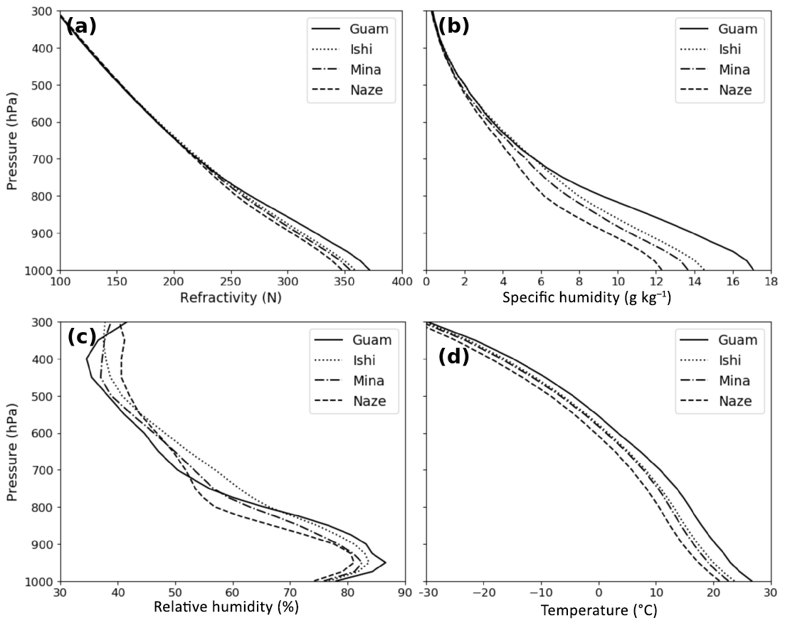
Figure 1 ERA annual average profiles on the 25 hPa grid for (a) refractivity, (b) specific humidity, (c) relative humidity, and (d) temperature at all four locations.

3 Results

3.1 Overview: general agreement and correlation between the data sets

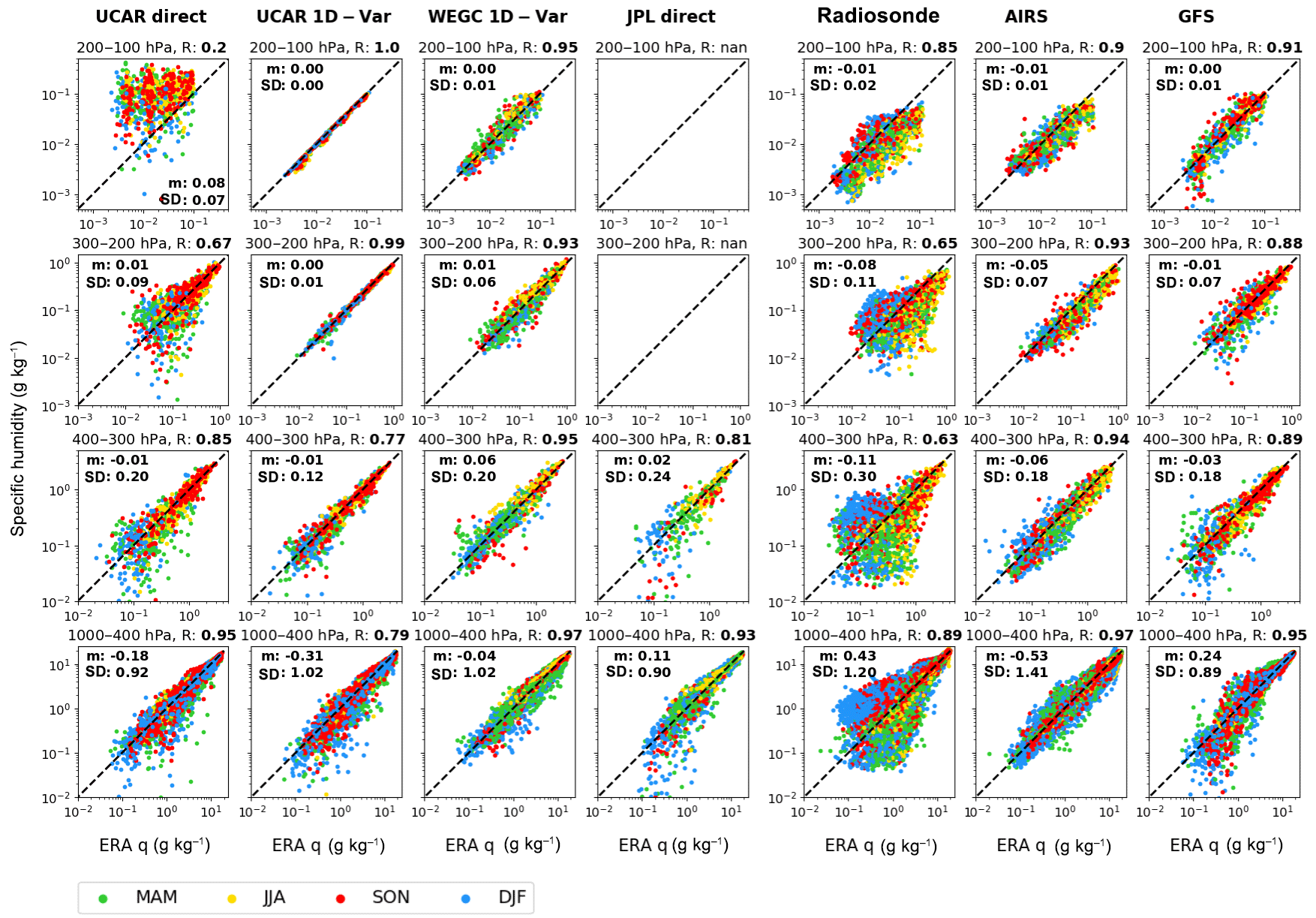
Figure 2 Guam: scatterplots of q for seven data sets versus ERA for four pressure layers. Left to right: UCAR direct, UCAR 1D-Var, WEGC 1D-Var, JPL direct, RS, and AIRS. Correlation coefficients as well as mean and standard deviation of the differences are given for each panel. Note that both axes are on a logarithmic scale and that axis limits vary for different pressure layers.

Figure 2 shows values of q for UCAR direct, UCAR 1D-Var, WEGC 1D-Var, JPL direct, RS, AIRS, and GFS (left to right) versus ERA from high- to low-pressure layers (top to bottom), depicting the correlation between the observational data sets and ERA at Guam (log–log correlation coefficients in the title of each panel). Additionally, the mean and standard deviation values of the differences for each pressure layer are depicted in each panel (since values are not normalized, values from the lower levels will have a larger influence on the result).

There is good agreement and high correlation for all data sets in the 1000–400 hPa layer (Fig. 2, bottom panels). The RS shows the largest difference (∼ 1 order of magnitude) for generally low humidity values. Some larger differences can also be seen for the UCAR direct, UCAR 1D-Var, JPL direct, and GFS when these data sets are much drier than ERA (primarily happening in the DJF season). The large differences occur generally for q values less than 1 g kg⁻¹, with many lower than 0.1 g kg⁻¹, which indicates dry higher altitudes (i.e., above 500 hPa). RO refractivity becomes less sensitive to water vapor at these higher altitudes, and the RO retrievals of water vapor, whether direct or 1D-Var, are less reliable at these levels (Kursinski et al., 1995). The UCAR 1D-Var can also have difficulties retrieving very low humidity values (which is the case in the DJF season at Guam). If the a priori temperature is too low, it can happen that the UCAR 1D-Var humidity values are set to zero, which would lead to a dry RO bias overall for low values of specific humidity. The data sets look similar in the 400–300 hPa layer, and a dry bias for the RS becomes visible. In the 300–200 hPa layer, the UCAR direct spread becomes very large (indicating limited usefulness for RO direct retrievals at this level), while the UCAR 1D-Var and WEGC 1D-VAR agree very well with ERA, since they are using ERA and ECMWF short-range forecast profiles as background in the retrieval, respectively. JPL direct humidity data are not available at these pressure levels. Both RS and AIRS show a dry bias. Finally, in the 200–100 hPa layer the UCAR direct data are useless, the UCAR 1D-Var is practically identical to ERA (simply recovering ERA a priori values), and the RS and AIRS data both have a strong dry bias. The GFS agrees fairly well with ERA in the upper layers and has no obvious bias.

3.2 Time series at Guam

Figure 3 2007 time series at Guam: (a) ERA relative humidity (%) with blue representing moist air and red representing dry air; (b) normalized difference of q (%) between PERSIST and ERA; (c) normalized difference of q (%) between GFS and ERA. The bottom panel shows that there are significant (±50%) differences in the two model data sets. The color bar on the right indicates relative humidity (%) in (a) and specific-humidity normalized differences (%) in (b) and (c).

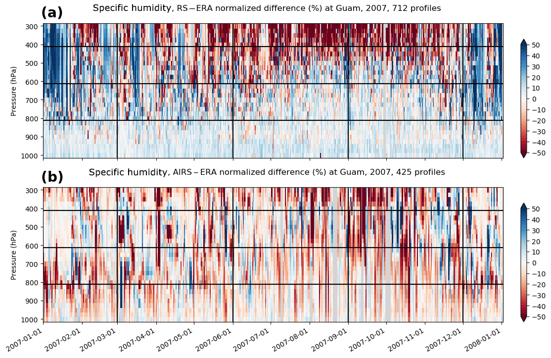
Figure 4 2007 time series of the q normalized difference between (a) RS and ERA, and between (b) AIRS and ERA at Guam. The color bar on the right indicates specific-humidity normalized differences (%).

Figure 3a shows the time–height cross section of RH over 2007 from 1000 to 400 hPa at Guam. Overall, the conditions at Guam are moist (RH > 80 % and q∼ 17 g kg⁻¹) year-round in the boundary layer and in the mid-troposphere from July to November, and dry in the mid-troposphere during the rest of the year. The changing humidity pattern above 800 hPa results from the alternation of the high-humidity tropical conditions and dry air intrusions from the subtropical UTLS in December to June (Randel et al., 2016). These dry intrusions (relative humidity as low as a few percent) are very stable and suppress convection. The sharp humidity gradient between the very dry lower mid-troposphere and the moist boundary layer around 800 hPa often leads to conditions of super-refraction, which results in a negative bias of N and thus q in the RO profiles (Xie et al., 2010).

The ND of specific humidity q between the PERSIST data set and ERA (which represents the day-to-day variability of ERA) shows that q has almost no day-to-day variability in the 1000–800 hPa layer during the entire year and in the 800–600 hPa layer in August and September (Fig. 3b). Above, day-to-day variability is significant. Exceptions occur in the 600–400 hPa layer during December through May, when persistent dry air intrusions occur. This shows just how stable and persistent these layers can be, suppressing major changes in humidity for up to 20 days in a row.

The ND of q between GFS and ERA (Fig. 3c) shows that the differences between the two model values of q are much smaller than the differences between PERSIST and ERA, as might be expected. GFS is up to 50 % moister than ERA in the 800–600 hPa layer in the dry season, and in the 800–550 hPa layer in the wet season. This is essentially the layer of strong humidity variability above the bottom layer of constant (about 80 %) relative humidity. This behavior may be due to GFS difficulties in capturing the sharp transition between dry and wet conditions on the bottom of dry layers in December to June. This is supported by individual profiles (e.g., Randel et al., 2016, Fig. 4), as well as our comparison of ERA with RS (Fig. 4a), which supports the ERA in this respect.

The ND show a small wet bias of the RS relative to ERA in the lower troposphere and large wet and dry biases in the middle and upper troposphere throughout the year (Fig. 4a). The large biases are likely caused by RS sensor malfunctions (Holger Vömel, personal communication, 2017), which can start as low as at 800 hPa. At some point during the ascent, the sensor gets stuck and keeps reporting the same humidity value, which manifests itself as a dry or wet bias compared to ERA, depending on if tropospheric conditions are drier (December through May) or wetter (June through November) than the incorrect reported value.

AIRS shows an overall dry bias compared to ERA throughout the entire troposphere in all seasons (Fig. 4b). The dry bias appears to be less during the dry-air-intrusion events in the 600–400 hPa layer in the dry season (December to June). This indicates that AIRS is less biased if the overall atmospheric conditions are dry. The AIRS dry bias agrees well with the findings of Wong et al. (2015), who studied the uncertainties of AIRS Level 2 Version 6 q and T depending on cloud types. They found reduced dry biases in the middle troposphere under thin clouds, but large dry biases (> 30 %) in the lower troposphere with low thick clouds, and dry biases throughout the troposphere in the presence of high thick clouds.

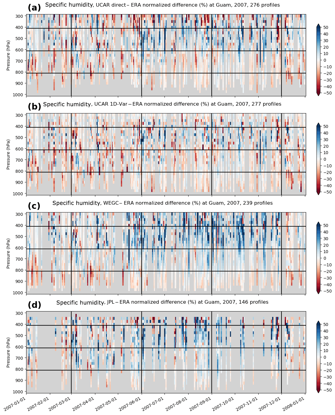
Figure 5 The 2007 time series of the q normalized difference at Guam for the (a) UCAR direct, (b) UCAR 1D-Var, (c) WEGC 1D-Var, and (d) JPL direct retrieval. The color bar on the right indicates specific-humidity normalized differences (%).

The normalized differences of the four RO retrievals to ERA show similar patterns in the 1000–800 hPa layer but larger differences in the mid- and upper troposphere (Fig. 5). The UCAR direct data develop a wet bias above 600 hPa in the wet season and alternate between dry and wet during the other seasons. The UCAR 1D-Var data show an overall dry bias throughout the troposphere with a few exceptions. Both JPL and WEGC data develop a strong wet bias above 600 hPa in the wet season. Common features of all four RO retrievals include the very small differences to ERA in the wet season in the 1000–800 hPa layer and a dry bias and/or frequent reduced penetration depth (loss of signal) in the dry season. The latter is a signature of super-refraction, which itself is caused by strong humidity gradients, usually between the planetary boundary layer and the free troposphere.

Figure 5 also shows that all RO data sets are biased dry with respect to ERA in December through February in the 800–600 hPa layer, which is clearly above the layer of strong humidity gradients (compare to Fig. 3a). We found similar behavior in previous work. In Rieckh et al. (2017), Fig. 2, lower right panel, ERA data are given on the 775, 750, 700, and 650 hPa pressure levels (about 2.3, 2.6, 3.1, and 3.8 km, respectively). The 775 and 650 hPa levels agree well with the aircraft and RO measurements; however, the two levels in between smear the sharp profile, and the ERA shows humidity values 1.5 to 2.5 g kg⁻¹ (20 to 35 %) larger than the observations. Thus we conclude that the bias in Fig. 5 may not be a dry bias in RO but could be a wet bias in ERA in the layer just above the strong humidity transition from wet (PBL) to dry (above). The assumed errors for assimilating RO in ERA are large in the lower troposphere, and all assimilated nadir-viewing instruments only provide vertical resolutions of about 2 to 3 km. Unless a nearby approved RS contributes information locally, ERA does not have any vertically well-resolved humidity data that will cause the ERA analysis to develop such sharp humidity gradients.

The 2007 time series of the q normalized difference for all data sets are depicted for a Japanese station (Minamidaitojima) in Figs. S5 and S6.

The 2007 time series of the refractivity N normalized difference for all data sets are depicted for Guam in Figs. S7 and S8.

3.3 Mean and rms differences from ERA at Guam

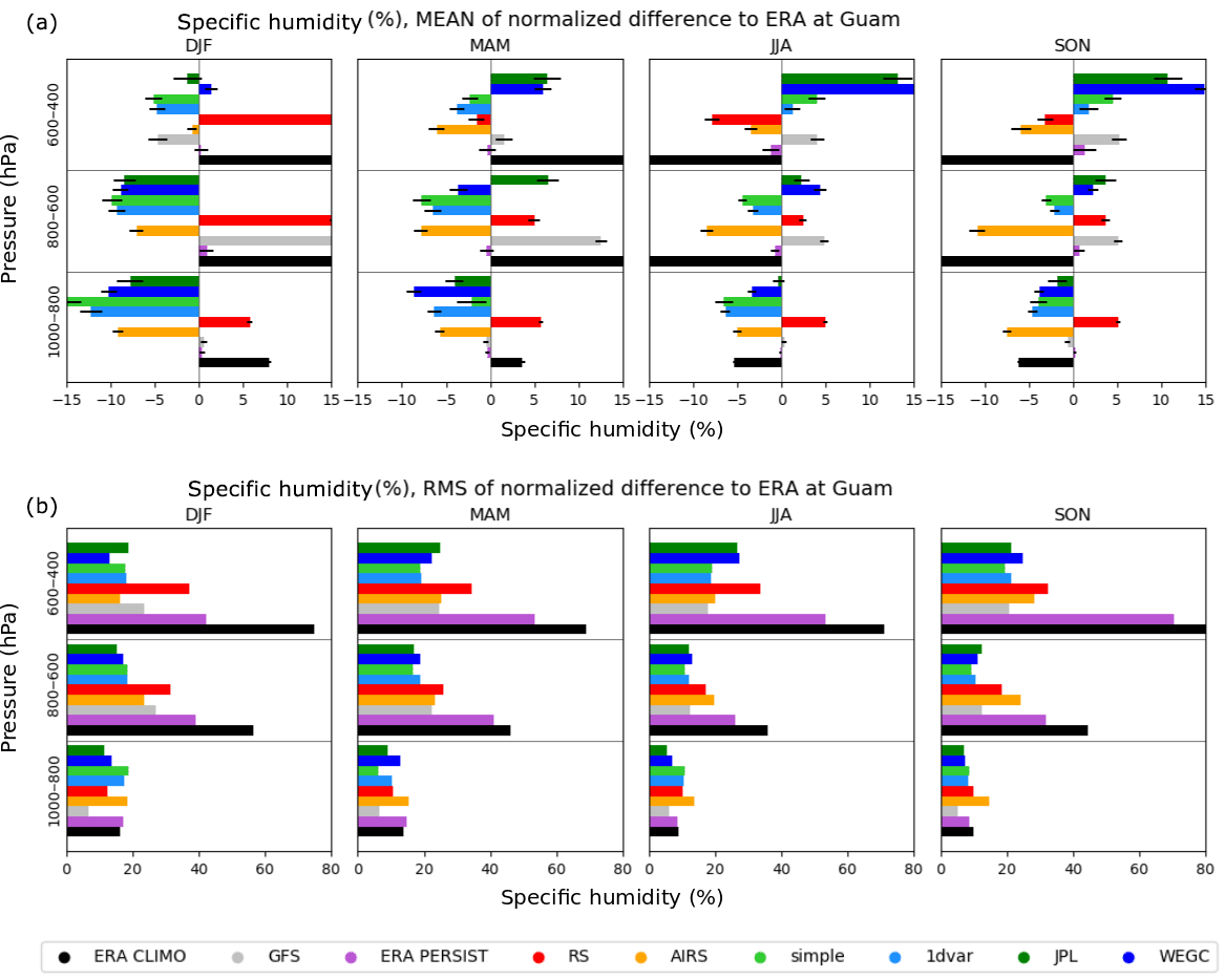
Figure 6 Guam: The mean (a) and rms (b) of the q normalized difference for all data sets, three pressure layers, and four seasons. Data sets from top to bottom (per pressure layer): JPL direct, WEGC 1D-Var, UCAR direct, UCAR 1D-Var, RS, AIRS, GFS, PERSIST, CLIMO.

We compute the mean and root mean square (rms) of the normalized differences at Guam to get a statistical overview of the differences from the ERA for all data sets for three pressure layers (1000 to 400 hPa in 200 hPa layers) and four seasons (Fig. 6).

Some general aspects of the different data sets seen in the individual time series are clearly visible in the mean (Fig. 6, top), such as the large negative (dry) difference of RO compared to ERA (green and blue bars) in DJF for the 1000–600 hPa layer. In the 1000–800 hPa layer, a dry bias for RO exists throughout the year. The dry bias is largest in DJF, but it is smaller than and comparable in magnitude to the biases of the RS and AIRS in MAM, JJA, and SON. RO retrievals show the greatest differences from each other in the 600–400 hPa layer year-round and in the 800–600 hPa layer in the wet season. AIRS shows an overall dry bias at all pressure layers and seasons. As expected, PERSIST has essentially no bias at any pressure layer or season. Because of the large seasonal variation in water vapor, CLIMO has large seasonal positive and negative biases above 800 hPa that are much larger than the biases of any other data set. GFS shows significant differences from ERA, especially in the dry season (DJF and MAM) in the 800–600 hPa layer.

Since the mean of the paired normalized differences is no indicator of their variability, we also show the rms (Fig. 6, bottom). The magnitude of the rms is a measure of the accuracy and scatter of the data compared to the reference. All data sets have a rms comparable to (below 800 hPa) or considerably smaller than (above 800 hPa) both CLIMO and PERSIST in all seasons (Fig. 6, bottom). The former is expected, considering how little humidity changes throughout the year in the 1000–800 hPa layer. The latter indicates the value (over persistence and climatology) of all observation techniques above 800 hPa. As for the individual data sets, we see that the RO rms for all retrievals is comparable to or lower than RS and AIRS rms for all seasons and pressure layers. This increases our confidence regarding the value of RO mid- and lower-tropospheric humidity data.

3.4 Statistics at the subtropical Minamidaitojima

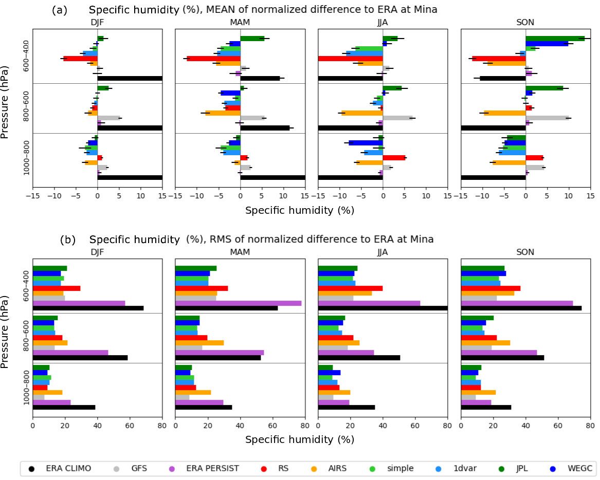
Figure 7 Mina: Mean (a) and rms (b) of the q normalized difference for all data sets, three pressure layers, and four seasons

At Minamidaitojima all data sets have a smaller bias compared to ERA (Fig. 7, top) than at Guam. The strong RO humidity bias in the dry-season lower troposphere (as seen at Guam) is not present, and biases of all observational data sets (with the exception of AIRS) are less than 5 % in the 800–600 hPa layer. Biases are larger in the 600–400 hPa layer, especially for the RS. The rms values at Minamidaitojima (Fig. 7, bottom) show a similar pattern to the one at Guam, with the RO and GFS rms differences being smaller than the RS and AIRS differences. The statistics of the other two Japanese stations (Ishigakijima and Naze) are similar (not shown).

4 Differences from ERA in dry versus wet atmospheric conditions

In Sect. 3 we saw how the general atmospheric humidity conditions (wet versus dry) can have an influence on the biases in the data sets with respect to ERA, especially for RO (super-refraction with strong vertical humidity gradients) and AIRS (smaller bias in dry conditions). In this section, we investigate the different error characteristics for dry and wet conditions in more detail at both the tropical and subtropical locations. We created a “dry” and “wet” data set. For every profile pair, we computed the average relative humidity (RH) of the ERA (background) profile for the 800–400 hPa layer (${\stackrel{\mathrm{‾}}{\mathrm{RH}}}_{\mathrm{800}-\mathrm{400}}$). This layer was chosen according to the humidity distribution throughout the year (see Fig. 3, top). If ${\stackrel{\mathrm{‾}}{\mathrm{RH}}}_{\mathrm{800}-\mathrm{400}}\le$30 %, the entire profile is added to the dry data set. If ${\stackrel{\mathrm{‾}}{\mathrm{RH}}}_{\mathrm{800}-\mathrm{400}}\ge$ 70 %, the entire profile is added to the wet data set. Then the mean and rms are computed for both these data sets separately. These statistical values are depicted for the 1000–800 hPa layer and the 800–400 hPa layer (Fig. 8).

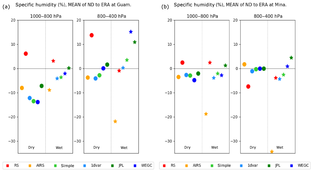
Figure 8 Mean differences for dry versus wet atmospheric conditions based on ${\stackrel{\mathrm{‾}}{\mathrm{RH}}}_{\mathrm{800}-\mathrm{400}}$ at Guam (a) and Minamidaitojima (b). The different colors represent the different data sets. Circles and stars represent the data sets for dry and wet conditions in the mid-troposphere, respectively.

The mean of the normalized differences shows different patterns for the dry and wet data sets at both Guam and Minamidaitojima. At Guam, we see a dry bias of 6 to 14 % in the 1000–800 hPa layer for all RO retrievals for the dry data set (Fig. 8, left). We assume that the dry air intrusions and sharp humidity transitions above the PBL with associated super-refraction conditions are primarily responsible for the negative N and thus negative q bias at Guam. The RO biases in the 800–400 hPa layer vary around zero (−4 to 2 %). For the wet data set, the mean RO differences from ERA vary significantly in the 800–400 hPa layer from 0 to 16 %, while the bias in the 1000–800 hPa layer is between 0 and −5 % for the RO retrievals. At Minamidaitojima, the RO data sets show smaller and similar biases for both pressure layers (Fig. 8, right). The dry RO data set has no bias in the 800–400 hPa layer and very small biases (2 to 5 %) in the 1000–800 hPa layer. The bias with respect to ERA of the wet RO data set ranges from −4 to 4 % in the 800–400 hPa layer and from −4 to 2 % in the 1000–800 hPa layer. Overall, we conclude that there are no major differences in the RO error characteristics between the dry and wet data sets or between the two pressure layers at Minamidaitojima, in contrast to Guam, where background humidity conditions clearly matter for the different error characteristics.

AIRS clearly shows a strong dry bias for both pressure layers for wet background conditions. The bias is stronger at Minamidaitojima, reaching more than −30 % in the 800–400 hPa layer and −20 % in the 1000–800 hPa layer. For dry conditions, the AIRS bias ranges from −8 to 2 % for all locations and pressure layers. This agrees well with the small bias seen in the regions of dry air intrusions (December to June) in the profile time series (Fig. 4, bottom).

Finally, the RS shows a small wet bias in the 1000–800 hPa layer for both the dry and wet data sets and both locations. In the 800–400 hPa layer, the dry data set shows a large wet bias, which is likely due to the Sippican VIZ-B2 sensor's poor performance in dry conditions (see Sect. 2.3). At Minamidaitojima, both the dry and wet data sets show a dry bias in the 800–400 hPa layer, as described in Vömel et al. (2007) for the Vaisala RS92 sensor for higher altitudes due to a radiation bias.

5 Variability during typhoon passages

We used the subtropical RS station Ishigakijima to investigate how the different data sets perform during the extreme conditions of typhoon passages. In 2007, six typhoons passed Ishigakijima within 350 km (the tracks and other details of the typhoons can be found online⁹):

• typhoon #4, 6–16 July, date of closest approach (320 km): 12 July, as typhoon category 4;

• typhoon #7, 4–10 August, date of closest approach (260 km): 7 August, as typhoon category1;

• super typhoon #9, 11–19 August, date of closest approach (300 km): 17 August, as typhoon category 4;

• typhoon #12, 11–17 September, date of closest approach (330 km): 14 September, as typhoon category 4;

• super typhoon #13, 14–20 September, date of closest approach (40 km): 18 September, as typhoon category 3;

• super typhoon #17, 1–8 October, date of closest approach (110 km): 6 October, as typhoon category 4.

The time series of differences to ERA q for Ishigakijima do not show a specific bias during typhoon passages, which indicates that all data sets as well as ERA report a signal similar in magnitude during the typhoon passages.

Figure 9 The q difference from CLIMO_JulOct for (a) GFS, (b) UCAR direct, (c) RS, and (d) AIRS shows increased humidity during typhoon passages near Ishigakijima. Typhoon passages are marked by vertical lines (dashed: closer than 110 km; dash-dotted: closer than 330 km).

We computed the ERA average over the July–October time range (CLIMO_JulOct) to create a typhoon season climatology. We then compared all data sets to CLIMO_JulOct to see how q and T deviate from the summer average during the passage of a typhoon. All data sets show a rapid increase in humidity (Fig. 9) and higher temperature values (not shown) as the typhoons approach and pass close to Ishigakijima. The signal is strongest above 600 hPa, where deep convection associated with the typhoons transports large amounts of water vapor and releases latent heat in the middle and upper troposphere (Emanuel, 1991).

GFS, RS, and all RO retrievals show similar results. The AIRS moist deviation during a passage is much weaker than for any other data set, likely because of all the cloud cover associated with the typhoons, which limits the AIRS retrievals.

All data sets show increased temperature during the typhoon event (not shown), especially in the upper troposphere. The UCAR and WEGC 1D-Var show a similar T structure. The signal also agrees well with the GFS T signal. Neither of the direct retrievals (UCAR and JPL) provides physical temperature information on the troposphere.

The signals in q, T, and N during a typhoon passage are similar for Minamidaitojima and Naze (not shown), but fewer typhoons passed in close proximity to these two stations.

6 Structural uncertainty of RO

Since we have data from several RO retrievals available, we have the opportunity to compute the structural uncertainty of RO humidity for our data set, following the methods of Steiner et al. (2013) and Ho et al. (2009, 2012). The structural uncertainty is computed to get an estimate of the variability among the various RO retrievals.

First we create sub-data-sets, which are limited to the profiles and pressure levels that are available for all four RO humidity retrievals. The sub-data-set for Guam consists of 141 profiles, and the sub-data-set for the combined Japanese stations (since atmospheric conditions are very similar among them) consists of 543 profiles. For each retrieval, the normalized deviation for N and q from the inter-center mean is computed (per pressure level):

$$\begin{array}{}\text{(5)}& \mathrm{\Delta }X={\displaystyle \frac{\mathrm{1}}{k}}\sum _k\left(X_k-{\stackrel{\mathrm{‾}}{X}}_k^{\text{inter-center}}\right){\displaystyle \frac{\mathrm{100}}{{\stackrel{\mathrm{‾}}{X}}_{\mathrm{annual}}^{\mathrm{ERA}}}},\end{array}$$

where k indicates the profile number, ${\stackrel{\mathrm{‾}}{X}}_k^{\text{inter-center}}$ is the inter-center average for the kth profile ($\mathrm{1}/\mathrm{4}(X_k^{\mathrm{UCAR}\mathrm{direct}}+X_k^{\mathrm{UCAR}\mathrm{1}\mathrm{D}-\mathrm{Var}}+X_k^{\mathrm{JPL}\mathrm{direct}}+X_k^{\mathrm{WEGC}\mathrm{1}\mathrm{D}-\mathrm{Var}}$), and ΔX is the deviation (of q or N) of one particular RO retrieval from the inter-center average.

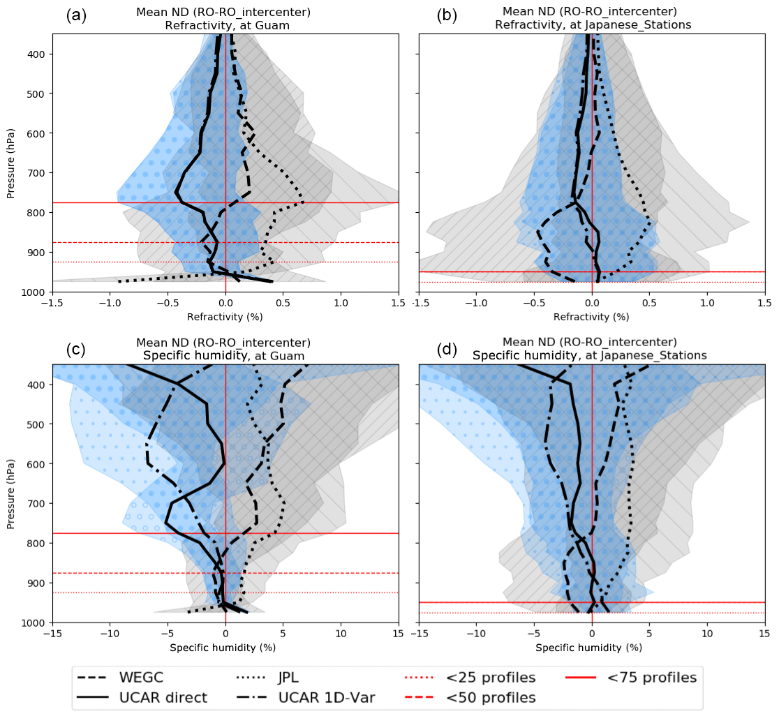
Figure 10 Deviations for four RO retrievals from the inter-center mean for refractivity (a, b) and specific humidity (c, d) at Guam (a, c) and the Japanese stations (b, d). The mean (and standard deviation) of each data set is shown by line style (and as shaded and hatched area): UCAR direct: black solid (and o o o, blue); UCAR 1D-Var: black dash-dotted (and $\cdot \cdot \cdot$, blue); WEGC 1D-Var: black dashed (and ///, gray); JPL direct: black dotted (and ∖ ∖ ∖, gray). Red horizontal lines indicate the number of profile pairs at that pressure level.

Figure 10 shows the mean deviations of the four RO retrievals from the inter-center mean for Guam (left) and all three Japanese stations combined (right) for N (top) and q (bottom). Cutoff pressure is 350 hPa since JPL does not provide humidity data above that level. For N (Fig. 10a, b), the absolute value of the mean deviation from the inter-center mean is largest between 900 and 700 hPa for all data sets (maximum of 0.7 %) and decreases to about 0.1 % at 350 hPa (about 8 km) at both locations. The latter result agrees well with the estimate of Ho et al. (2009), who showed that the absolute values of fractional N anomalies among four centers (UCAR, WEGC, JPL, and GFZ (German Research Centre for Geosciences)) are 0.2 % from 8 to 25 km altitude. The larger differences between the various RO processing centers at lower altitudes primarily come from different handling of profiles experiencing (1) atmospheric multipath, (2) receiver tacking errors, and (3) super-refraction (see Ho et al., 2009, for details on the RO processing center procedures). This is especially true for direct retrievals (such as the UCAR direct and JPL direct), where both RO N and a priori T are assigned zero error, and the differences in Fig. 10a and b are dominated by the previously mentioned conditions. For 1D-Var retrievals, another potential source of differences is the N error model in the respective 1D-Var retrieval. All these factors vary with latitude and general atmospheric conditions.

For q (Fig. 10c, d), the structural uncertainty generally increases with increasing altitude (since the impact of water vapor on N decreases with increasing altitude). At Guam, it is about 2 % in the PBL, increases sharply to 5 % around 800 hPa, and stays around 5 to 8 % above. At the Japanese stations, the structural uncertainty increases constantly with increasing altitude, from 2 % close to the surface to 5 % at 400 hPa. At both locations, the center anomalies increase sharply at 350 hPa, which indicates again that RO-derived humidity has high uncertainty at and above that level.

7 Conclusions

We compared three observational data sets (RO, RS, and AIRS) and two model data sets (ERA and GFS) over the year 2007. Rather than comparing averages over larger timescales and regions, we compared individual profiles over specific locations (in the tropical and subtropical west Pacific). The data sets that were compared to ERA, which we considered the reference data set, include profiles from four different RO retrievals (UCAR direct, UCAR 1D-Var, WEGC 1D-Var, JPL direct), RS, AIRS, GFS analysis, ERA PERSIST, and ERA CLIMO (the last two to set a quality baseline). We studied both the time series of profile pairs and the mean and rms computed for the four seasons and three pressure layers (1000 to 800, 800 to 600, and 600 to 400 hPa). As expected, we found different characteristics for each data set. Our main conclusions are as follows:

1. For all four RO humidity retrievals, the magnitude of the mean biases relative to ERA is smaller than or comparable to those of the RS and AIRS in the 800–400 hPa layer. Above 600 hPa, differences between the various RO humidity retrievals generally become larger (Figs. 6 and 7, top).

2. All data sets have smaller rms differences than both CLIMO and PERSIST (Figs. 6 and 7, bottom). The exception is the tropical 1000–800 hPa layer, where all rms values are comparable in magnitude due to the nearly constant humidity conditions throughout the year. This confirms that all observational data sets contribute valuable information compared to persistence and climatology.

3. The rms of all RO retrievals is comparable to or lower than the rms of the RS and AIRS for all pressure layers below 400 hPa, which confirms the high quality of RO profiles (Figs. 6 and 7, bottom). The agreement among the four different retrievals of specific humidity in the lower and middle troposphere validates the stability of the four retrievals.

4. In the time series, the four RO retrievals agree within 10 % in the 1000–600 hPa layer (Fig. 5). Differences become larger in the 600–400 hPa layer, where the UCAR 1D-Var gets drier, the UCAR direct alternates between too dry and too wet, and both the WEGC 1D-Var and JPL direct become too wet. Since water vapor decreases exponentially with altitude, the retrieval becomes more and more sensitive to the prescribed temperature, which can lead to larger humidity differences.

5. The structural uncertainty of RO humidity retrievals is estimated from anomalies of RO retrievals from the inter-center mean. Maximum differences among retrievals from 1000 to 400 hPa are between 1 and 0.2 % for refractivity, and 3 and 10 % for specific humidity (Fig. 10).

6. RO has the potential to contribute valuable information on water vapor via data assimilation in the mid- and lower troposphere, especially when high-quality RS are unavailable (Southern Hemisphere, over oceans). In contrast to infrared or microwave sounders, RO can resolve strong vertical gradients of humidity.

7. AIRS is biased dry throughout the entire troposphere, as noted previously (Wong et al., 2015). This bias is particularly strong for wet atmospheric conditions (Fig. 8).

8. All data sets show increased humidity and temperature values during a typhoon passage (Fig. 9). Differences from ERA do not change noticeably during a typhoon passage, indicating that all data sets and ERA report a signal that is similar in magnitude during the typhoon passages.

We find that the alternating wet and dry seasons at Guam, together with the very sharp transition at the top of the planetary boundary layer in the dry season at Guam, are especially challenging for the RO, RS, and AIRS observational systems compared to the conditions at the subtropical Japanese locations. The results comparing the different data sets to the ERA are similar at the three Japanese RS stations.

All the observational data sets at the Japanese stations show a response to the rapid increase of water vapor throughout the troposphere during the passage of typhoons; however, the AIRS response is weaker than the RS and RO responses, probably because of the extensive clouds associated with the typhoons.

Our results support the findings of Vergados et al. (2018), e.g., the relative dryness of the UCAR 1D-Var and wetness of the JPL RO humidity retrieval, and the dry bias of AIRS. While Vergados et al. (2018) draw their conclusions from large-scale multi-year climatologies, we use high-resolution time series to depict the short-term and small-scale variability of humidity, and we add results below 700 hPa, where the tropospheric water vapor content is highest.

We conclude that the accuracy of RO humidity retrievals is comparable to or better than both standard RS and AIRS data at the four tropical and subtropical locations studied here above 800 hPa, as well as below 800 hPa if super-refraction is absent. If assigned smaller errors (and therefore greater weights) in the assimilation process, RO could have a positive impact on improving the water vapor analysis in data assimilation in the lower and mid-troposphere.