the Creative Commons Attribution 4.0 License.
the Creative Commons Attribution 4.0 License.
 | 06 Jun 2018
Design, construction and commissioning of the Braunschweig Icing Wind Tunnel
Stephan E. Bansmer
Arne Baumert
Stephan Sattler
Inken Knop
Delphine Leroy
Alfons Schwarzenboeck
Tina Jurkat-Witschas
Christiane Voigt
Hugo Pervier
Biagio Esposito
Beyond its physical importance in both fundamental and climate research, atmospheric icing is considered as a severe operational condition in many engineering applications like aviation, electrical power transmission and wind-energy production. To reproduce such icing conditions in a laboratory environment, icing wind tunnels are frequently used. In this paper, a comprehensive overview on the design, construction and commissioning of the Braunschweig Icing Wind Tunnel is given. The tunnel features a test section of 0.5 m × 0.5 m with peak velocities of up to 40 m s−1. The static air temperature ranges from −25 to +30 ∘C. Supercooled droplet icing with liquid water contents up to 3 g m−3 can be reproduced. The unique aspect of this facility is the combination of an icing tunnel with a cloud chamber system for making ice particles. These ice particles are more realistic in shape and density than those usually used for mixed phase and ice crystal icing experiments. Ice water contents up to 20 g m−3 can be generated. We further show how current state-of-the-art measurement techniques for particle sizing are performed on ice particles. The data are compared to those of in-flight measurements in mesoscale convective cloud systems in tropical regions. Finally, some applications of the icing wind tunnel are presented.
- Article
(30827 KB) - Full-text XML
- BibTeX
- EndNote


Atmospheric icing affects the operational performance of many man-made devices and ground structures. Examples include icing of electrical power networks (Farzaneh, 2008), wind turbines (Hochart et al., 2008), communication towers (Mulherin, 1998) and aircraft (Gent et al., 2000).
Based upon the understanding of the physics and chemistry of clouds (Lamb and Verlinde, 2011), several icing mechanisms are well-known to atmospheric scientists and engineers: supercooled droplet freezing (Jung et al., 2012) – including freezing drizzle and rain (Zerr, 1997), snow accretion (Makkonen, 1989) and mixed-phase icing (Currie et al., 2012). Particularly, in the field of aircraft icing, supercooled large droplet (SLD) icing with median droplet diameters above 50 µm is considered as an independent category (Politovich, 1989).
Supercooled means that the droplets are in a metastable liquid state although their temperature is below the freezing point. Solidification can take place through homogeneous or heterogeneous nucleation. In absence of any impurities like aerosols, homogeneous nucleation starts with exceeding a barrier of free enthalpy triggering the creation of critical embryos. The change of free enthalpy is a function of latent heat of fusion (promoting phase change) and energy needed to create a new water–solid interface (hindering phase change). With increasing supercooling the latent heat of fusion increases thus making homogeneous nucleation more probable. Droplet impact on a solid substrate promotes heterogeneous nucleation initiating a fast development of ice dendrites in the liquid (Schremb and Tropea, 2016).
The following important parameters are of particular significance in defining the boundary conditions of the icing process:
-
Classical, fluid-mechanical testing parameters like Reynolds number , Mach number and angle of attack α, where ϱair is the density and μair the dynamic viscosity of air, U∞ the free-stream velocity, c a reference length of the test model and a∞ the speed of sound. All kind of test models can be considered for this dimensional analysis, e.g. aircraft, airfoils, probes, et cetera.
-
Water concentration in the air. On the one hand, this is the liquid water content (LWC), a measure of the mass of water per unit volume of air. Typical values for atmospheric icing conditions range from 0.1 to 3 g m−3 and have been measured in the updraft of continental convective systems e.g. above the Amazon basin; see Wendisch et al. (2016) and Braga et al. (2017). On the other hand, in the presence of ice crystals, the ice water content (IWC) has to be specified. Inside continental and oceanic mesoscale convective systems, IWC values are about 1 g m−3 (Gayet et al., 2014). While ice water content in mid-latitude cirrus is generally low (Voigt et al., 2017), peek values of 6 g m−3 have been observed in deep convective systems. Commonly, total water content (TWC) is defined as the sum of LWC and IWC.
-
Median volume diameter (MVD) of the statistical distribution of water droplets in the liquid cloud. MVD attempts to reduce the size distribution to a single, representative scalar diameter. This idea is attributed to Langmuir (Finstad et al., 1988; Langmuir, 1961). In the presence of ice crystals, a median mass diameter (MMD) is defined because of their variable density.
-
Static air temperature for water droplet icing close to 0 ∘C promote glaze ice formations, whereas rime ice formation becomes predominant at lower static air temperatures (Wagner, 1997).
-
Humidity, i.e. the amount of water vapour in the air, is an important parameter for mixed-phase ice accretion (Currie et al., 2012). Jung et al. (2012) showed its relevance for pure droplet icing. A distinction is made between absolute humidity AH and relative humidity RH. Absolute humidity is defined by the mass of water vapour per unit volume of dry air. With the partial pressure of water vapour pvapour, the static air temperature Tair and the specific gas constant of the vapour Rvapour, this yields . Relative humidity is defined as the ratio of the partial pressure of water vapour pvapour to the equilibrium vapour pressure of water , i.e. .
-
Accumulation time tacc, for which the test model is exposed to the cloud of supercooled droplets and/or ice crystals.
Among the above enumeration of boundary conditions, temperature is of particular importance, because it governs the freezing dynamics of impacting supercooled water droplets. At very low temperatures, the droplets will solidify shortly after their impingement and entrap the surrounding air. The resulting ice accretion is called rime ice. With increasing temperature, the solidification process of impacting droplets is retarded, yielding wind-driven water film dynamics. At locations with increased convective heat transfer, the water film freezes, yielding a nearly transparent – glaze ice shape with typical horn formations.
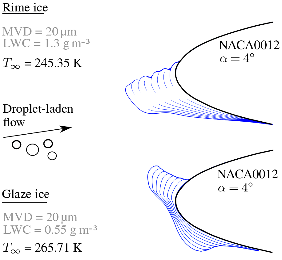
Figure 1Rime ice and glaze ice shapes over time at the leading edge of a NACA0012 airfoil, chord length 0.53 m. One blue line represents one minute of ice accretion. Further boundary conditions (rime): U∞=58 m s−1, tacc=8 min; (glaze): U∞=102.8 m s−1, tacc=7 min. Data from computations with TAUICE by Jan Steiner.
The choice of boundary conditions for conducting a specific icing wind tunnel experiment depends on the application under investigation. When testing to support industrial product developments, certification requirements often define the boundary conditions. In Europe, icing of large transport aircraft is addressed in the document CS25 (EASA, 2016) of the European Aviation Safety Agency (EASA). In its Appendix C, information on the standard LWC–MVD envelope can be found, where the liquid water content is in the range between 0.1 and 2.9 g m−3 and MVD between 15 and 50 µm. Icing certification for wind energy converters is governed by the technical standards of the International Electrotechnical Commission (IEC). Among others, the Det Norske Veritas Germanischer Lloyd (DNV GL) is an accredited registrar and classification society responsible for certification of wind energy converters, having created calculation rules and detailed specification based on the IEC; see GL (2010). It has to be noted that industrial products are in many cases significantly larger than the dimension of a typical icing wind tunnel. Hence, appropriate scaling laws are necessary to overcome the limited ranges of air speed, test section dimension and icing cloud characteristics in icing wind tunnels (see Bond and Anderson (2004)).
Besides supercooled droplet icing, the aircraft industry has become aware of another icing hazard in the recent past. The phenomenon called “ice crystal icing” has been identified to effect ice accretion on heated aircraft assembly such as engine compressor blades or stagnation pressure probes. Thrust losses and engine damages as well as biased flight parameter display and loss of the autopilot can be caused. Ice crystal icing mostly appears in tropical regions in the vicinity of convective cloud systems. A comprehensive treatment on the topic was published by Mason et al. (2006). The Federal Aviation Administration (FAA) of the United States and EASA extended their icing regulations to Appendices D and P for ice crystal icing conditions in 2010 and 2011. Enhanced research activities on the topic have been promoted lately by NASA (Flegel and Oliver, 2016) and the National Research Council of Canada (Currie et al., 2014).
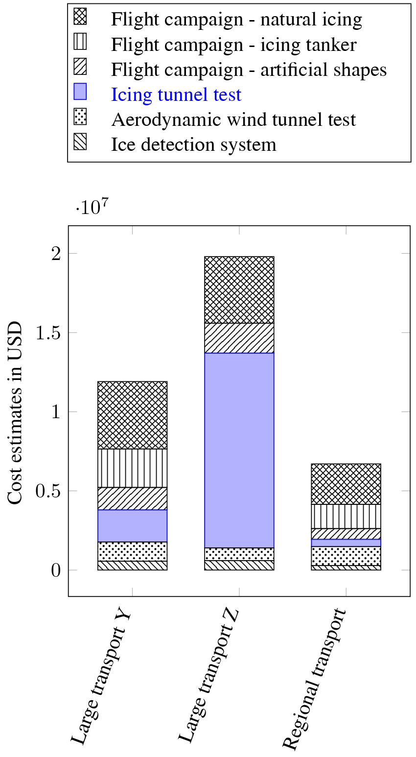
Icing is a very challenging field of study that incorporates aspects of meteorology, fluid mechanics, thermodynamics, physics and engineering. Despite the fact that many researchers have been involved in the study of ice accretion over numerous decades, the physics of this phenomenon is still not completely understood. Icing wind tunnels are therefore an essential pillar to advance our knowledge in face of this multidisciplinary challenge. Enduring changes in technical standards or certification processes to continuously improve the safety against icing related incidents further emphasize the industrial need for icing wind tunnel testing. The cost estimations of the Ice Protection Harmonization Working Group (IPHWG) for aircraft certification with respect to SLD-icing underlines this requirement; see Fig. 2.
Against this background, the design and construction of the Braunschweig Icing Wind Tunnel began in 2010. It was a goal to contribute a tunnel with sufficiently large dimensions in the test section to support both fundamental and applied icing research with reasonably low operating costs. During the design, construction and commissioning process, many lessons have been learned, which can not be found in the literature and thus form the outline of this publication. The major components of the Braunschweig Icing Wind Tunnel and their design constraints are presented in Sect. 2. The special topic of mixed phase icing, where both supercooled droplets and ice crystals are involved in the icing process, is treated in Sect. 3. Together with the international co-authoring partners, the commissioning of the tunnel was realized, which is presented in Sect. 4. Finally, some applications and test results that show the tunnel's capabilities are highlighted, with some concluding remarks on health and safety considerations.
2.1 Overall design
The aim to build a low-budget icing wind tunnel for research purposes influenced major choices on the operational envelope. The main targets in icing wind tunnel design are to obtain a homogeneous distribution of flow velocity, temperature, and a uniform icing cloud in the test section. Therefore, it is the test section that governs the design choices.
The first choice was on the dimension of the test section. Addressing customers in aviation, automotive and energy industries requires reasonable aerodynamic testing where the wind-tunnel wall boundary layers are significantly smaller than the size of the test section. In this regard, investigations with Reynolds numbers up to 2×10⁶ are a frequent demand. Moreover, the test section shall allow for mounting significant aircraft subsystems and particle sizing instrumentation. Hence, a cross section of 0.5 m × 0.5 m was considered as a lower bound for sizing the icing wind tunnel. Additionally, it has to be taken into account that the test section size is in relation with the overall dimension of the icing wind tunnel. The space available at the installation site suddenly becomes a further design constraint.
The maximum velocity is primarily determined by the power of the wind tunnel drive; see Sect. 2.2. However, when considering the heat balance in icing wind tunnels (see Sect. 2.3) the importance of the chilling device becomes evident. Figure 3 shows cost estimations for both drive and cooling power, which is based on price lists of leading manufacturers in their respective fields. Realizing that the cost for tunnel cooling is about 10 to 20 times more expensive than for the tunnel drive, the maximum velocity in the test section is in direct relation to the available investment costs for building the tunnel. Given an upper bound for the tunnel drive power, a compromise between test section size and maximum velocity has to be made. Consistent with the above requirements of test section size, the maximum velocity was estimated to be 40 m s−1. A larger test section size would decrease the maximum velocity given a constant drive power. Since many aeronautical applications even demand for higher speeds, the decisions of a maximum velocity of 40 m s−1 and a test section of 0.5 m × 0.5 m were taken.
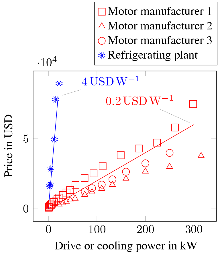
Figure 3Pricing as of 2017 for asynchronous motors from different manufactures and for CO2 refrigerating plants before tax and tolls.
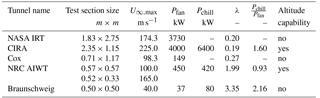
The lower temperature limit inside the test section was set to −20 ∘C. Below this bound, one usually observes rime ice accretions on the test models. In contrast, glaze ice formation with temperatures closer to 0 ∘C is significantly more complex from the perspective of fundamental research that shall be conducted in the present icing wind tunnel. An overview of the entire tunnel and its adjacent components is given in Fig. 4. A comparison with the specifications of selected other icing wind tunnels can be found in Table 1.
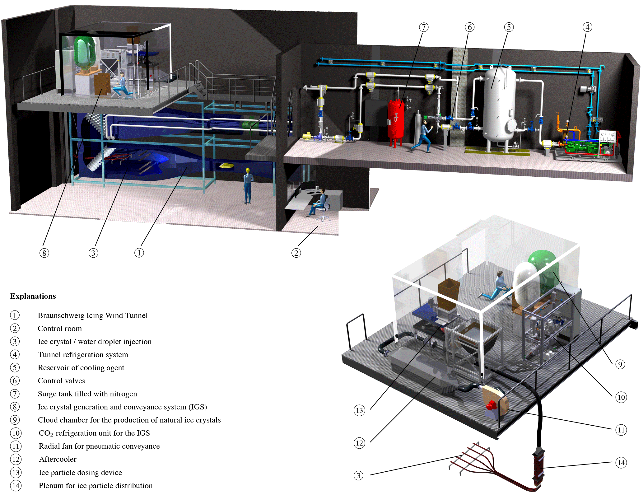
Table 1Performance of different icing wind tunnels compared to the Braunschweig Icing Wind Tunnel. U∞,max represents the maximum air speed in the test section, Pchill is the installed cooling power. Data extracted from Pastor-Barsi et al. (2012), Vecchione and De Matteis (2003), Al-Khalil et al. (1998) and Oleskiw et al. (2001).
2.2 Tunnel drive
Given an air temperature of −20 ∘C, a maximum speed U∞ and a cross-sectional area Atsec of the tunnel test section, the required jet power Pjet can be calculated to the following:
In wind-tunnel design, a power factor λ is introduced, which indicates the ratio of fan power Pfan and jet power Pjet. For a conventional, closed-loop, low-speed wind tunnel, a value of λ≈1.5 can be assumed. The fan power has to compensate pressure and skin friction losses of the individual tunnel components. High losses are caused by the wall boundary layers of the test section and the tunnel diffuser. Furthermore, the first and the second corner after the diffuser create significant losses. Since the vanes of the first corner are subject to ice accretion, their losses are tremendously high compared to conventional closed-loop tunnels. Consequently, the power factor was dimensioned to a large value of λ=2.3, yielding a fan power of Pfan ≈ 25 kW. An axial fan with an efficiency ηfan≈ 67 % was selected for the tunnel drive, the electrical power input is therefore 37 kW. Using a frequency converter, the speed of the three-phase asynchronous motor of the fan drive can be controlled, allowing variable tunnel speeds from 5 to 40 m s−1.
2.3 Chilling device
To adjust and maintain a constant temperature of the air inside the icing wind tunnel, which is well below the freezing point of water, a chilling device is necessary, whose cooling capacity has to exceed the power of the wind tunnel drive.
2.3.1 Power estimation
There are three major heat sources that have to be compensated by the chilling device: the power of the tunnel drive, the heat input through the wind-tunnel walls and the heat transfer of the water spray. The latter is composed of the sensible heat, to supercool the water spray from the temperature at which it leaves the pneumatic atomizer (about 20 ∘C) down to the air temperature inside the tunnel test-section and the latent heat . As soon as the supercooled water droplet impacts on a solid substrate, the drop solidifies due to the heterogeneous nucleation and releases the latent heat. Both sensible and latent heat are a function of the liquid water content:
where is the water mass flow rate of the spray atomizers and ΔT the temperature difference, with the values for demineralized water as follows:
For typical operational conditions of the icing wind tunnel, i.e. U∞= 40 m s−1, ΔT= 30 K, and approximations for the fan power and the heat input through the wind-tunnel walls, the necessary cooling capacity can be estimated; see Fig. 5. When LWC is in the range of 1 g m−3, a continuous cooling power of 30 kW is necessary. To allow for a five minute peak load of LWC = 3 g m−3 and static air temperatures down to −20 ∘C in the tunnel, the system was dimensioned for a maximum cooling power of 80 kW.
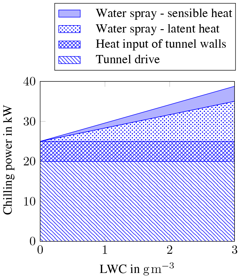
Figure 5Required chilling power decomposition as a function of the liquid water content for typical operational conditions of the Braunschweig Icing Wind Tunnel.
2.3.2 Refrigeration unit
To provide the icing wind tunnel with 30 kW continuous cooling capacity and 80 kW maximum cooling capacity, a customized cooling unit was built (see the upper right part of Fig. 4). The core of the system is a refrigeration unit, ➃, that cools the heat transfer fluid (Therminol® D12) down to a temperature of −32 ∘C. To compensate for the volume change of the fluid, a surge tank, ➆, filled with nitrogen is installed. The cold fluid is then stored in a 4 m3-sized buffer tank, ➄, which acts as a hydraulic switch; on its right side, it is connected to the refrigeration unit. On its left side, it is connected to the heat exchanger in the wind tunnel. As a result, the operation of the refrigeration unit is decoupled from the heat exchanger in the wind tunnel. Using a pump and electrically operated valves (➅), the volume flow from the buffer tank to the heat exchanger in the wind tunnel is controlled. Depending on this flow rate, the continuous cooling power of 30 kW of the refrigeration unit can be well exceeded. For a 80 kW peak load operation, the complete buffer tank is first cooled to −32 ∘C, and afterwards the chilled heat transfer fluid is pumped through the heat exchanger at the wind tunnel within a short period of 7 min. The recovered waste heat from the cooling process is fed into the regenerative heating system of the institute building. Because of its cold-resistant properties, the piping of the cooling system and the storage tanks are made of stainless steel 1.4541, and then insulated with a 4 cm thick insulation layer made of Kaiflex®. The entire system is controlled by programmable logic control.
2.3.3 Heat exchanger
The heat transfer between the Therminol® D12 fluid and the circulating wind tunnel air takes place through two consecutive heat exchangers. While flowing from the bottom to the top of the first heat exchanger, the Therminol® D12 fluid increases in temperature. With only one heat exchanger, this would yield an undesired vertical temperature gradient in the passing air flow. The second compartment, in which the Therminol® D12 fluid flows the opposite way, thus compensates the vertical gradient in air temperature. The entire assembly is installed in front of the third corner in the wind tunnel, see also the illustration in Sect. 2.9. The large distance to the test section promotes a homogenization of the temperature distribution over the tunnel cross-section through turbulent effects.
Mechanically, the heat exchangers have a cross-sectional area of 1.6 m × 1.6 m and are composed of elliptical tubes made of stainless steel and rectangular, smooth steel fins, which are firmly connected to each other by hot galvanizing. The fin pitch is 3.5 mm. To protect the galvanized steel surface against corrosion, it is coated with ZACOSIN® 2000Q, an epoxy resin-based protective coating that provides high thermal conductivity by embedded aluminium particles; see also Sect. 2.8. Alternatively, the heat exchanger could also have been made entirely of stainless steel. However, compared to standard steel, stainless steel has a significantly lower thermal conductivity (50 compared to 15 ), which is why the surface of the heat exchanger would have to be much larger.
The heat exchangers also include a condensation drainage. Condensation occurs predominantly in the initial cooling phase from room temperature to cold operational temperatures. When continuously running at low temperatures, the effect of condensation is only minor.
2.4 Settling chamber
To obtain a low turbulence level inside the test section of the tunnel, a settling chamber with honeycomb and screens is installed. An influence on the longitudinal (parallel to the main flow direction) and lateral flow structures (perpendicular to the main flow direction) has to be distinguished (Scheiman and Brooks, 1981). The honeycomb reduces both the lateral components of mean velocity and of the larger turbulent eddies, whereas the screens reduce the longitudinal components of turbulence or mean-velocity variations across the sectional area. For the Braunschweig Icing Wind Tunnel, a combination of screen–honeycomb–screen–screen was selected. The screens have a mesh size of 6 mm, the honeycomb diameter is 10 mm, its length is 100 mm.
2.5 Spray system
A spray system is required to produce a uniform drop distribution in the tunnel test section. In the past five years, two different spray systems have been developed; one system suited for large droplets (MVD ≈ 80 µm) and a high liquid water content (1.1 g m−3 3 g m−3) and a second spray system for low MVD (8 µm 48 µm) and low LWC (0.1 g m−3 2 g m−3).
The spray system for large droplets is composed by a grid of 5×5 air-assisted atomizers. Inside one atomizer, a thin jet of water is destabilized by the shear forces of a transversely directed air stream and finally breaks down into small droplets. The diameter of the water jet, which is in the range of 100 µm, determines the water volume flux as well as the drop size. The higher the applied air pressure, the higher the aerodynamic shear forces, and the smaller the drop size. In order to enable a high variability of the drop size distribution for basic tests, the atomizers are designed in a modular manner, that is, the water jet and the air atomizer cap can be exchanged separately.
Stainless steel has been chosen as a material for the atomizers, since otherwise conventional atomizers made of nickel-plated brass are prone to wear due to frequent temperature changes inside the icing tunnel (from +20 to −20 ∘C). However, the poor thermal conductivity of stainless steel (15 ) compared to brass (120 ) has to be considered. Since the spray atomizers are directly exposed to the cold tunnel air, they would freeze without corresponding countermeasures. Therefore, a heating coil is installed close-by.
The high liquid water content (1.1 g m−3 3 g m−3) provided by the spray system is a technical constraint of air-assisted atomizers. Below a certain water flow rate that is needed for low LWC, their operation becomes unstable. This is because the low water pressure inside the atomizer cap prevents the formation of a stable water jet, which is needed prior to atomization. The second spray system circumvents that problem and was specially designed for low liquid water contents; see Fig. 6. To achieve a LWC of 0.1 g m−3, a water volume flux can be estimated to the following:
Using a spray matrix of 5×5 atomizers, this yields a volume flux of 0.14 L h−1 per atomizer, which is ten times lower than the typical minimum flow rate of air-assisted atomizers in industrial environments. In consequence, electrically actuated air-assisted atomizers have been chosen for the spray system. The atomizers are pulsating up to 10 000 times a minute, making the spray appear to be constant. By changing the duty cycle, the LWC can be adjusted without modifying the pressure of water and air supply, which is a major advantage compared to classical air-assisted atomizers.
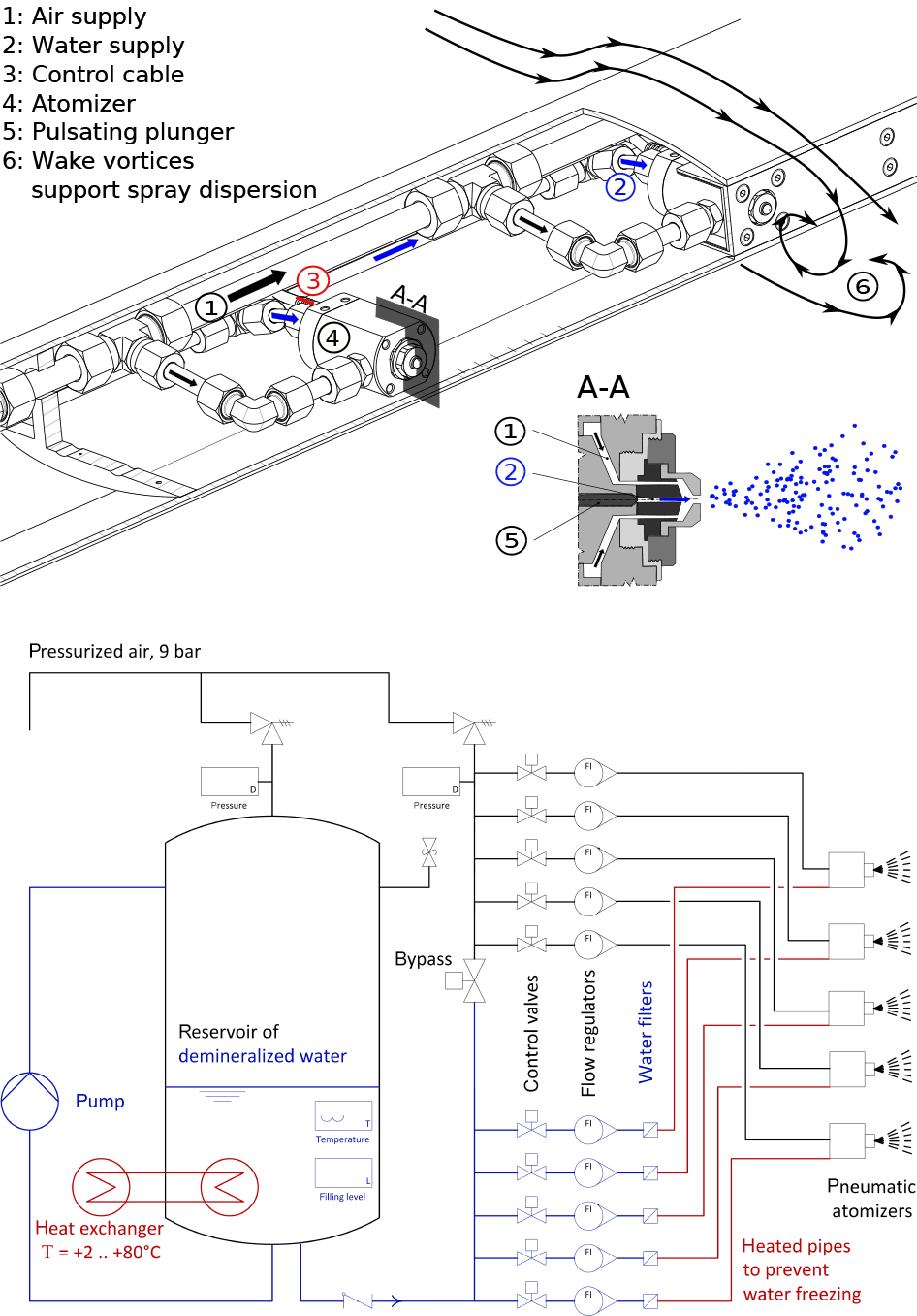
Water and air are conditioned for the operation of the air-assisted atomizers; see again Fig. 6. A pressurized vessel of stainless steel serves as a reservoir of water, whose temperature can be regulated between 2 and 80 ∘C. Water pressure and air pressure can be adjusted separately between 0.5 and 9 bar. Water flow rate and air flow rate are measured and adjusted by flow regulators. Possible pollutant particles, which could block the nozzles, are separated with water filters. In larger icing test facilities, where tunnel air temperatures below −40 ∘C can be adjusted, the air duct of the spray atomizers is heated in order to prevent droplet freeze out. In our setup, droplet freeze out is less likely due to the minimum temperatures of around −20 ∘C, which are well above the homogeneous nucleation limit of water. Therefore, the atomizer's air duct is not heated and air at room temperature is used to operate the atomizers.
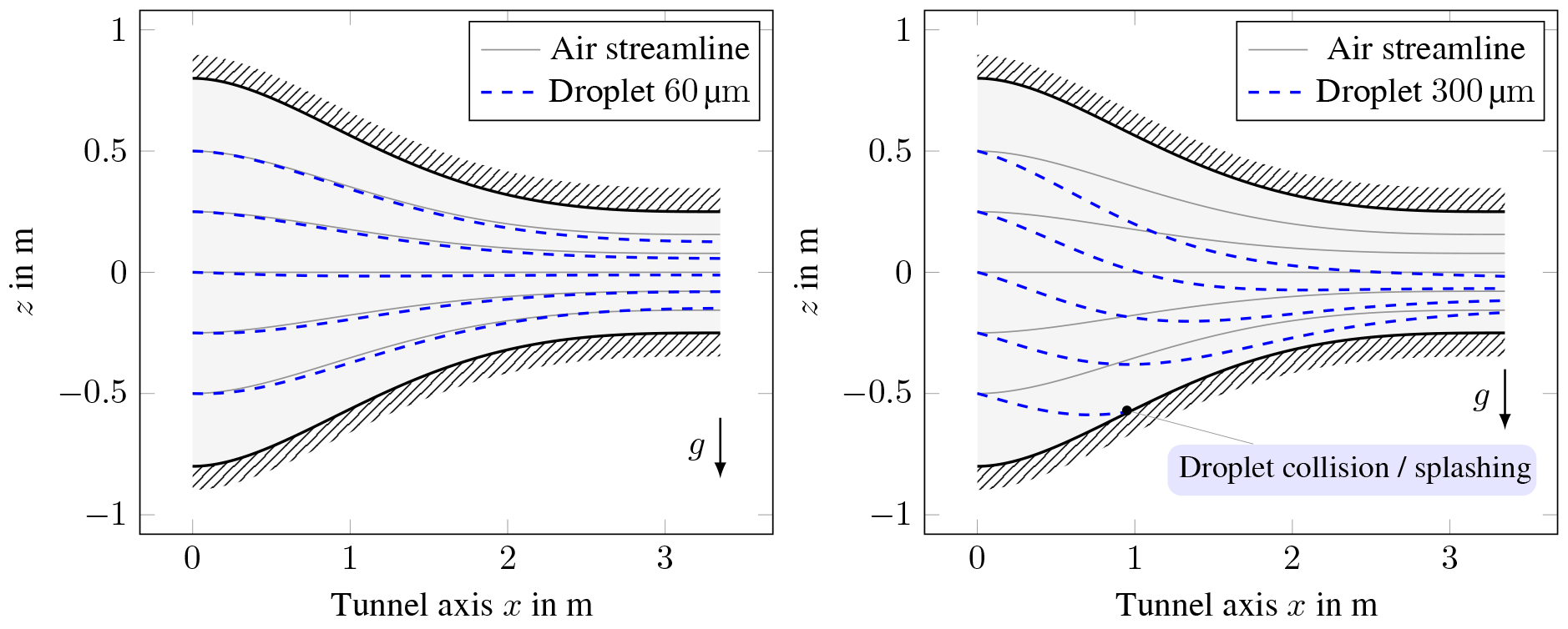
Figure 7Droplet trajectories in the wind tunnel nozzle and their deviation from the air streamlines under the influence of gravity. Large droplets may collide with the tunnel walls thereby altering the droplet size distribution.
2.6 Tunnel nozzle design
Having passed the settling chamber, the flow is accelerated in the tunnel nozzle that contracts towards the dimensions of the test section. Beyond altering the turbulence structure (Uberoi, 1956), the shape of the tunnel nozzle also influences the trajectories of the water droplets that are injected by the spray system. Especially large droplets and ice particles are affected.
Two different nozzle geometries have been considered. These are the following:
-
the AVA nozzle, with its contour given by the following:
-
the Witoszynski nozzle, with its contour given by the following:
where x,z are spatial coordinates, L is the nozzle length, zsc,ztsec are half of the inlet and outlet diameter of the nozzle and K is given by . To provide enough time for the supercooling process of the droplets on their way to the tunnel test section, a large nozzle length of 3.5 m is foreseen.
The droplet trajectories are mainly governed by inertial forces, drag and gravity. A water droplet with diameter d, velocity vector is transported by the air velocity resulting in a drag force of the following:
where represents the slip velocity. Assuming laminar flow around the spherical droplets with a mass of md at low Reynolds numbers , the drag coefficient cD can be approximated to . Applying the principle of d'Alembert, this yields a system of differential equations, given by the following:
where t represents the time and g is the acceleration due to gravity.
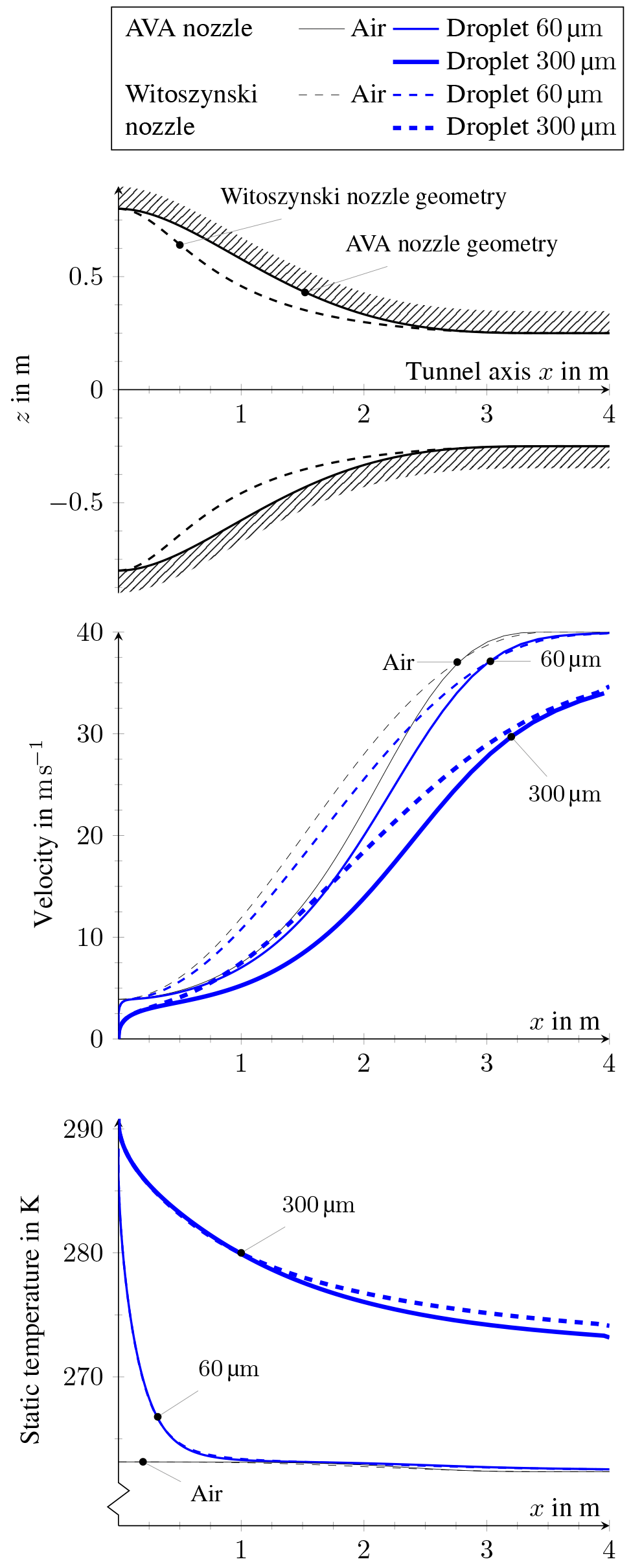
Figure 8Velocity and temperature slope for air and two different sized droplets inside two tunnel nozzle configurations.
The effect of gravity on the droplet trajectories is depicted in Fig. 7, assuming an air velocity of 40 m s−1 at the nozzle exit. Small droplets with a size of 60 µm follow the streamlines of air flow inside the nozzle. With increasing droplet size, the gravitational deflection becomes predominant, particularly at the low speed regions of the nozzle. For 300 µm droplets, their trajectory from the lowest spray bar even collides with the nozzle wall. Such undesired collisions alter the size distribution of the droplet cloud and have to be avoided.
Figure 8 demonstrates the effect of the nozzle geometry on the droplet slip velocity. Note that after the nozzle length of L= 3.5 m, a straight segment of 0.5 m in length is attached. In the low speed region x< 1.5 m, the AVA nozzle accelerates the flow less than the Witoszinski nozzle. Consequently, the slip in velocity between droplet and air is larger in that region. Downstream, for x>3 m, the slip is caught up. While the small droplet of 60 µm approaches the air speed of 40 m s−1 when entering the test section at x = 4 m, the large droplet of 300 µm still has a slip of about 5 m s−1. Different initial droplet velocities created by the air-assisted atomizers were considered likewise. However, we observed that the surrounding low speed air flow in the settling chamber rapidly decelerates the droplet. This effect on the droplet trajectory is thus negligible in our tunnel.
Furthermore, the cooling process of the droplet on its trajectory has to be considered. Cooling is promoted by a convective heat transfer at the interface between droplet and air. When the droplet is smaller than 100 µm, the surface temperature penetrates the entire droplet volume in about ten milliseconds, assuming a Fourier number of 1 for the heat conduction problem; see also Yao and Schrock (1976). Hence, isothermal cooling can be assumed as an approximation for the thermal energy balance, yielding a differential equation for the droplet temperature Td:
where ϱd and cp,d represent the density and the specific heat capacity of the droplet, kair is the heat conductivity of air and Nu is the Nusselt number, estimated by ; see Knudsen and Katz (1958). Herein, Pr=0.7 is the Prandtl number of air.
Using the above equation, the temperature evolution of the droplet inside the tunnel nozzle is plotted in Fig. 8 for a given static air temperature of Tair=263.15 K. After one metre travelling distance, the droplet of 60 µm, which had an initial temperature of Tair=293.15 K, has already reached the air temperature. In contrast, the droplet of 300 µm has still a temperature above the freezing point of water, when entering the test section at x= 4 m.
In summary, droplet conditions up to a maximum size of 150 µm can be well provided in the present tunnel environment, taking into account a reasonably low deflection due to gravity, a low slip velocity and sufficient droplet cooling. Furthermore, the AVA geometry was selected for the wind tunnel nozzle, because it enables a slightly higher heat transfer to supercool the droplets.
2.7 Tunnel walls
2.7.1 Mechanical design

To minimize the heat transport through the wind tunnel walls, they consist of three different layers with a total thickness of 80 mm; see Fig. 9. Between two layers of aluminium, an insulating foam with low heat conductivity is introduced. The inner aluminium shell which is potentially exposed to the icing cloud is anodized for a protection against corrosion. The flange of each wall segment is made of purenit®, a highly compressed material based on PUR/PIR rigid foam providing a high thermal insulation. A rubber seal prevents the water from penetrating into the wall. The flanges were fastened with many screws, thus avoiding water leakage. In order to make the joints fully watertight, the inner groove was sealed with an acrylic compound. Due to an excellent manufacturing accuracy, no steps between adjacent wall segments are observed.
2.7.2 Aerodynamic wall effects
Icing wind tunnel tests usually involve models with large dimensions to minimize uncertainties when applying scaling laws for ice accretion. The flow around these models thus interferes with the walls of the test section. Two different wall effects have to be considered. On the one hand this is the viscous effect of junction flow (Simpson, 2001), which occurs when the boundary layer of the wind tunnel wall encounters the test model attached to the same wall. The adverse pressure gradient forces the wall boundary layer to separate with horseshoe vortices that wrap around the obstacle. These unsteady vortices result in high turbulence intensities, high surface pressure fluctuations and heat transfer rates, which finally alter the ice accretion in that area. This effect was computationally studied for a NACA0012 airfoil with the icing code FENSAP (Beaugendre et al., 2003); see Fig. 10. FENSAP solves the Reynolds-averaged Navier–Stokes equations using a finite element approach, calculates droplet trajectories with an Eulerian scheme and finally determines the ice accretion using a model of Messinger (1953). The upper part of Fig. 10 clearly identifies the horseshoe vortex while plotting the spanwise velocity in multiple slices and an isosurface along the NACA0012 airfoil. Especially in the vicinity of the leading edge at the junction between airfoil and wind-tunnel wall, the two-dimensional flow behaviour is significantly deteriorated. Because a glaze ice case was simulated (T∞ = −10 ∘C, LWC = 1 g m−3, ice accumulation time tacc=120 s), the velocity field strongly influences the heat transfer. At the junction, the decreased heat transfer attenuates the ice accretion, which is shown in the lower part of Fig. 10. However, the two-dimensional ice shape distant to the tunnel wall, which covers 80 % of the wing span, remains unaffected.
The second case of wind-tunnel wall interaction is an inviscid effect. The distant walls that are not connected to the test model will influence the streamlines around the model. Thereby, both pressure and shear stress distribution along the model surface are altered. Interestingly, at low speeds and sufficiently large droplet sizes (MVD = 15 µm), the ice accretion is nearly unaffected, when tunnel walls are introduced; see the computational results of the icing code TAUICE in Fig. 11. TAUICE is developed by the German Aerospace Center. It solves the Reynolds-averaged Navier–Stokes equations using a finite volume approach, calculates droplet trajectories with a Lagrangian scheme and finally determines the ice accretion using a model of Messinger (1953).
2.8 Corrosion
Since the operation of the icing wind tunnel entails the usage of water droplets or ice particles, corrosion has to be considered during the design process. The most vulnerable part of the tunnel in this regard is the heat exchanger, as it is made from a mix of steels, which is galvanized together; see Sect. 2.3.3. Without any proper protection, many factors decide on the rate of corrosion of a galvanized surface, the most important for this application being the chemical composition of the water and the type of surface contact.
Water with a high content of carbonates supports the creation of a protective layer of alkaline zinc carbonates ZnCO3 on the galvanized surface. However, with no or only few carbonates and a relatively high content of oxygen, the water reacts with the zinc to form zinc hydroxide . This further forms a compound 2 ZnCO3⋅3 Zn(OH)2, also known as white rust, which does not have the protective function of zinc carbonates, but only connects loosely to the surface. Similar to normal rust this porous layer keeps water near the surface and delays drying, which further increases the rate of corrosion. Over time, particles flake off, until the zinc is used up.
The type of surface contact between water and the galvanized surface is important for the rate of corrosion. If the water is sprayed onto the surface and remains as small droplets, each droplet forms a small corrosion element with a large surface that promotes the supply of oxygen. This increases the corrosion rate in comparison to the case where a galvanized surface is completely submerged in water with only a small contact area to the surrounding air.
To protect the galvanized steel surface of the heat exchanger against corrosion, it is coated with ZACOSIN® 2000Q, an epoxy resin-based protective coating that provides high thermal conductivity by embedded aluminium particles.
Another metal in contact with the deionized water is brass, which is used in several valves, pipe connections, etc. Brass forms tarnish, a thin dark layer of stable metal oxides, that protects the base metal. Unlike rust, the oxidation reaction is self limiting. As soon as the layer is formed, no more metal is oxidized. The tarnish did not pose any problem in all parts.
The models for the tunnel are made from aluminium or glass-fibre reinforced plastics (GRP). None of these materials showed any signs of reaction with the water so far. The same holds for the inner wall of the wind tunnel which is made of anodized aluminium. Even with scratches from installing models no signs of corrosion showed up.
2.9 Basic instrumentation
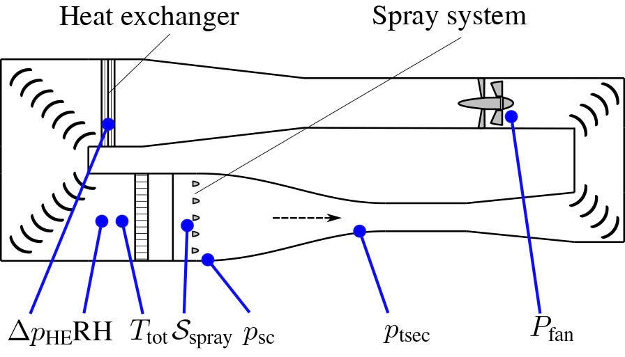
To monitor the icing wind tunnel operation and thus the boundary conditions of an experiment, several probes are necessary; see Fig. 12. The velocity U∞ in the test section is determined by two static pressure probes psc and ptsec. Their typical accuracy for long term stability is ±0.3 % of the full scale output. Using the Bernoulli equation:
where usc is the velocity in the settling chamber at psc, ϱair is the density of air, ζnozzle is the specific loss coefficient of the wind tunnel nozzle, and a continuity equation as follows:
where Asc and Atsec are the cross sectional areas of settling chamber and test section, one can estimate the following:
Note that the effect of pressure losses in the wind tunnel nozzle is usually neglected, since and ζnozzle≪1.
A Vaisala HMT-337 monitors both the relative humidity RH and the total temperature Ttot in the settling chamber. The uncertainty for the humidity measurement is ±1.8 % RH, the accuracy for the temperature measurement is around ±0.3 ∘C. Ttot is used to calculate the static air temperature T∞ in the test section,
where cp,air is the specific heat capacity of air. Moreover, the temperature information is necessary to determine the density ϱair of air in Eq. (2). The power of the tunnel drive Pfan and the pressure loss over the heat exchanger ΔpHE indicate the performance degradation of the icing wind tunnel due to ice accretion. Furthermore, the state of the spray system 𝒮spray is controlled; see Sect. 2.5.
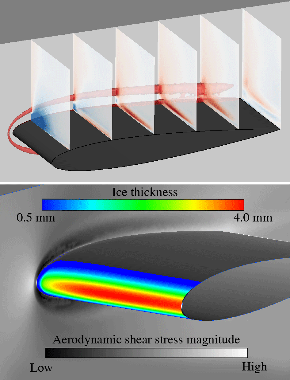
Figure 10The junction flow between a NACA0012 airfoil (c=0.75 m, α=0∘) and wind-tunnel side wall creates a horseshoe vortex (upper image), which is altering the ice accretion (lower image). U∞=40 m s−1, ∘C, LWC = 1 g m−3 and IWC = 0.
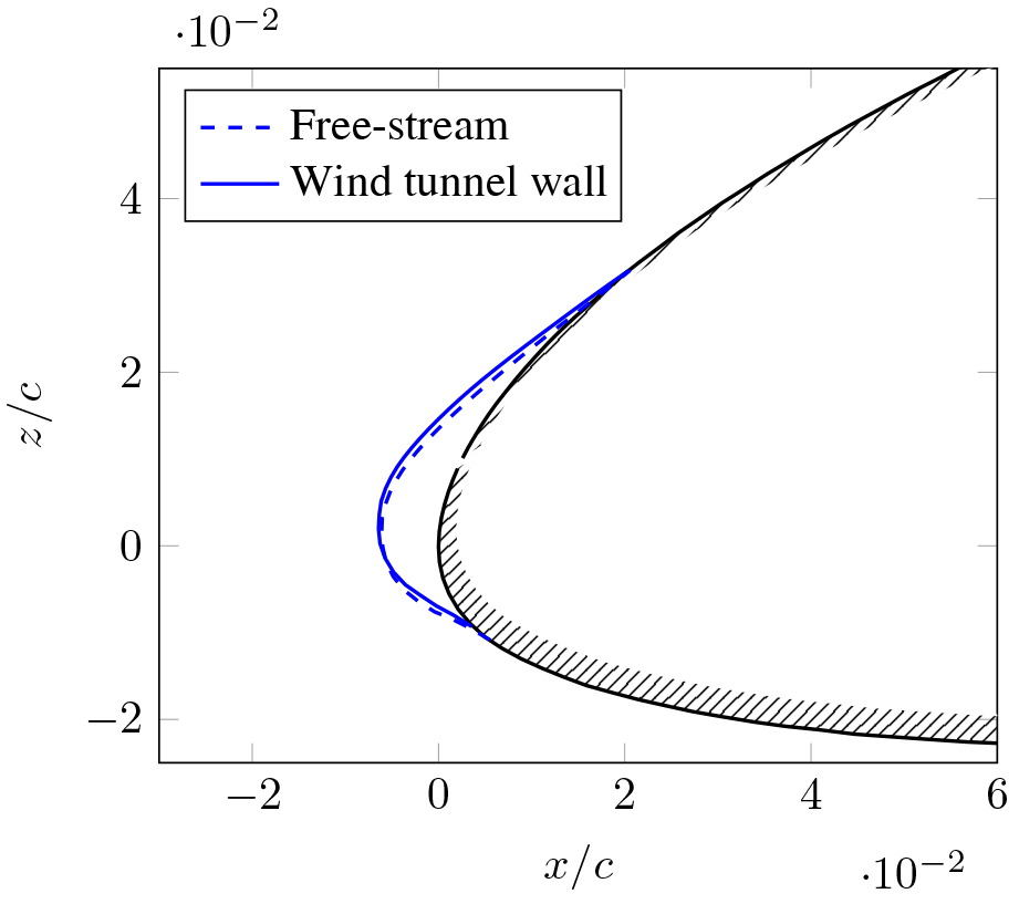
Figure 11Inviscid wall effect on ice accretion for a AH-94-W-145 airfoil, c=0.75 m, U∞=40 m s−1, ∘C, LWC = 0.3 g m−3, MVD = 15 µm and IWC = 0.
Ice crystals in the atmosphere have to be considered for aircraft safety, since they partially melt in warm environments and develop a “sticky” character. In particular, heated stagnation pressure probes and engine compressor stator blades can be maleffected by ice crystal icing (Mason et al., 2006). Icing of aircraft probes can cause false flight parameters displayed inside the cockpit. Ice accretion inside the compressor causes flow blockage, forcing the compressor to operate towards stall conditions. The compressor encounters a decay in rotational speed resulting in significant thrust losses (rollback event) (Oliver, 2014). Moreover, total engine flame out may appear if a huge mass of accumulated ice is shed into the combustor.
To provide experimental capability on ice crystal icing, the Braunschweig Icing Wind Tunnel was upgraded with an ice crystal generation and conveyance system, which is presented in this section; see also Fig. 4.
3.1 Morphology of ice crystals
Ice crystal icing conditions are typically encountered in wide ranging convective cloud systems of high ice water content at flight altitude. Such conditions can especially be found in the vicinity of mesoscale convective cloud systems in tropical regions; see Grzych and Mason (2010) and Leroy et al. (2015). In order to better document ice crystal icing conditions, two flight campaigns have been conducted in the course of the HAIC and HIWC project (Dezitter et al., 2013; Strapp et al., 2016). The first campaign took place in Darwin, Australia, in 2014 during the monsoon period, the second campaign in Cayenne, French Guiana, in 2015 during the rainy season. The flight measurements have been conducted in high ice water content cloud areas in large tropical mesoscale convective systems, mostly over the oceans. Details about the campaigns and about data treatment can be found in Leroy et al. (2016a), Leroy et al. (2016b) and Leroy et al. (2017).
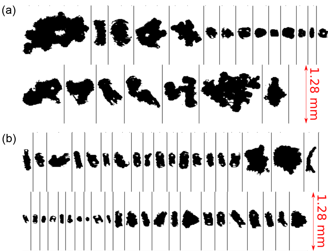
Figure 13Ice particle images captured by 2D-S probe during the Darwin Campaign. (a) Stratiform cloud region, MMD ≈ 150 µm, IWC ≈ 1.2 g m−3, T∞≈ −10 ∘C. (b) Convective cloud region, MMD ≈ 80 µm, IWC ≈ 3 g m−3 and T∞ ≈ −10 ∘C.
Atmospheric ice particles feature a broad diversity of sizes and shapes which depend on the individual ice particle growth history affected by ambient temperature and super-saturation. Figure 13 (a) shows examples of ice particle images captured close to −10 ∘C during the Darwin campaign with the 2-D-Stereo probe (see Sect. 4.5 for a description of the instrument). Images from Fig. 13 correspond to a stratiform part of the cloud where rather constant ice water content close to 1.0 g m−3 was sampled. Images from Fig. 13 (b) were recorded in convective cores with IWC peak values exceeding 3 g m−3. In the convective part, ice particles are more numerous and smaller. Close to −10 ∘C, column and capped column type crystals have been found. Larger ice particles (> 600 µm) are rare and resemble graupel (dense and roundish particles). On the contrary, in the stratiform part of the cloud, ice particles larger than 600 µm are more frequent and appear to be less fragile, consisting of aggregates of pristine shapes. Since particle growth is affected by vapour deposition and aggregation and encounters different temperature regimes, a lot of different and irregular shapes are possible at all altitudes in mesoscale convective cloud systems.
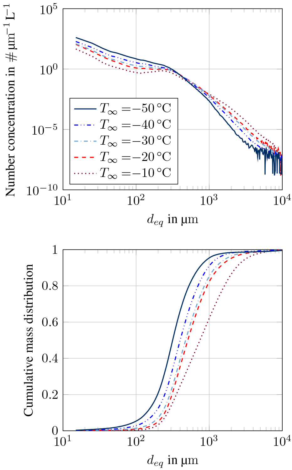
Figure 14Ice particle size distribution (MMD) based on HAIC Falcon 20 flight measurements from Darwin and Cayenne in dependence of ambient air temperature.
Figure 14 shows ice particle size and mass distributions (PSD and MSDs) depending on ambient temperature using the equivalent diameter deq for size definition. The equivalent diameter intends to provide a size information on a non-spherical particle. It is defined as the diameter of a circle of the same area as the shaded pixel number for each particle. With the distribution of deq it is therefore possible to compare the composition of icing clouds in both atmosphere and icing wind tunnel environment. The size and mass distributions have been averaged for the selected temperature regimes, only cloud areas with total water content above 1.0 g m−3 have been taken into account. The concentrations of small (< 200 µm) and large (> 1 mm) ice particles vary in opposite ways with temperature: for colder temperatures, concentrations of small ice particles increase, whereas the number of large particles decreases (cf. Fig. 14). This temperature dependency might be a consequence of several cloud processes. Nucleation of new ice particles is favoured at low temperatures, creating new small ice crystals. On the opposite, growing of ice crystals by collection processes requires larger particle sizes and might be more efficient at higher temperature. Regarding the dynamics of the cloud, small ice particles can also easily be carried aloft by updraft winds. Therefore, there is still no clear and unique scenario describing the formation of high IWC areas in clouds. Cumulative ice particle mass distributions are plotted in the bottom part of Fig. 14. PSDs have been converted in to MSDs, following the work of Fontaine et al. (2014) and Leroy et al. (2016b). Bin masses are linked to the particle size using a power-law relationship . However, β and γ are not constant; for each time step, γ is deduced from the analysis of particle images and β is constrained by additional TWC measurements, thus ensuring that the total mass from the MSDs equals the measured TWC. With decreasing atmospheric temperature, the cumulative particle mass is carried more and more by small ice particles. The median mass diameter (MMD), reduces from roughly 750 µm at −10 ∘C to 320 µm at −50 ∘C. More details about MMDs in high IWC cloud regions can be found in Leroy et al. (2017).
As mentioned above, ice crystal icing can cause malfunctions of aircraft engines due to inner ice accretions. Inside-engine conditions are characterized by ice particle sizes of about 20 µm as ice particles fragment in the fan stage. Due to centrifugal forces, high ice particle concentrations can be found in the casing region of the core engine. The local TWC can exceed the atmospheric TWC by a factor of 4 or even more; see Feulner et al. (2015).
3.2 Ice crystal production in a cloud chamber
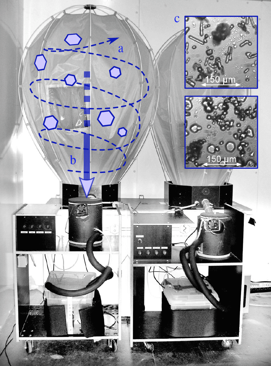
Figure 15Ice crystal generators. A jet of air (a) circulates the flow, allowing for ice crystal growth. When the crystals are large enough, they fall into a chest freezer (b). Microscopic images of ice particles inside the cloud chambers (c). Both plate crystals and needles can be generated.
It has been aimed to reproduce closest possible replicates of natural ice crystals. Cloud chamber technology has been identified to be appropriate, because natural ice crystal growth is simulated in an artificial cloud. Usually, cloud chamber technology is applied in meteorological science to investigate ice crystal formation and growth mechanisms and to study the interaction of individual ice crystals; see Connolly et al. (2012). Thus, the productivity of cloud chambers is accepted to be rather low. For icing wind tunnel studies, huge amounts of ice particles are required. In collaboration with the Austrian Neuschnee GmbH, two highly productive cloud chambers have been developed and installed inside a cooling room. Figures 4 and 15 show both cloud chambers and auxiliary equipment. Basically, atomized droplets are forced to freeze out inside the chamber by the expansion of cool pressurized air. Strong circulation of air keeps the particles in suspense until they grow to certain size and settle down to the bottom of the chamber. The production rate of the cloud chamber is not sufficient to enable a direct supply of ice crystals into the wind tunnel. Thus, the particles are collected inside a chest freezer, which is directly connected to the cloud chambers. The chest freezers operate at −70 ∘C to minimize degeneration and sintering of the particles. Currently, the production rate for both cloud chambers is limited to about 1 kg h−1. This production rate is sufficient to perform between 10 to 15 wind tunnel tests a day.
Microscopic images of ice crystals grown inside the cloud chamber are shown in the upper right part of Fig. 15. The primary ice particle habit can be adjusted by variation of ambient temperature inside the cooling chamber. After storing in the chest freezer, the ice particles typically feature aggregates of individual crystals as further illustrated in the following section.
3.3 Ice crystal conveyance
To establish defined cloud conditions inside the test section of the icing wind tunnel, ice particles are fluidized into an airflow and guided into the wind tunnel; see Fig. 4. The conveying airflow is extracted from the icing wind tunnel by a bypass construction including a radial fan. An external heat exchanger (aftercooler) cools the air to compensate heat input of the fan and environment. The aftercooler is connected to the refrigeration system of the cooling chamber. Downstream of the heat exchanger, the piping system enters the cooling room where ice particles are supplied to the airflow. Further downstream, the particle-laden flow is discharged into the icing wind tunnel.
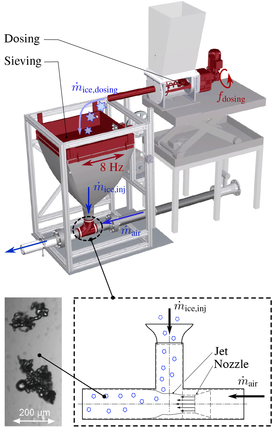
Figure 16Assembly for ice particle dosing and fluidization. Ice particle structure after storage, dosing and sieving procedure.
To adjust the ice water content inside the test section a defined mass-flow of ice particles has to be supplied at a constant feed rate. Particle dosing is realized by a volumetric dosing machine, shown in Fig. 16. The dosing machine has a very linear operating behaviour: the higher the frequency of the dosing machine motor, the higher the supplied ice particle massflow; see Fig. 17a. After storage and dosing, the particles are partially interlocked and exist as accumulated ice clumps, which are by far larger than the desired particle sizes of several tens of microns. Thus, the particles have to be sieved to desired sizes, which is realized by a custom made sieving machine; see again Fig. 16. The sieving machine is driven by an electric motor that forces a 800 mm × 800 mm sieve to oscillate at a frequency of 8 Hz. The total mass of ice provided by the dosing machine does not pass the sieving machine. Greater clumps of ice are not fully broken by the sieving procedure and depose on the sieve. The average deposit is about 15 to 20 % of the ice mass provided by the sieving machine.
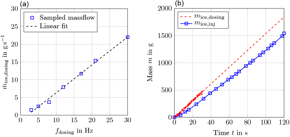
Figure 17Ice particle massflow, (a) dependence on dosing machine frequency and (b) ice particle supply over time at a dosing frequency of fdosing=21 Hz.
The sieving machine is connected to the conveyance piping system by a conical flexible bag. Ice particles passing the sieve directly fall into the piping system and get dragged by the pipe airflow. To adapt the local pressure inside the piping system to the ambient pressure inside the cooling room, the piping system implies an injector nozzle that induces a local jet inside the pipe; see the lower part of Fig. 16. The nozzle diameter is carefully adjusted based on preliminary calculations of the pressure distribution inside the whole piping system. The temporal stability of the mass flow is depicted in Fig. 17b. The dashed line shows the ice particle mass supplied by the dosing machine at a frequency of 21 Hz. It is a linear fit, a constant feed-rate has been proven by weighing, as indicated by the red data points. The blue dots and the solid blue line represents masses of ice weighed at the outlet of the sieving machine. This curve shows a very linear behaviour as well. One can conclude that after about 30 s the ice particle massflow injected into the wind tunnel is temporally constant. Weighing of ice mass passed by the sieving machine has been repeated several times, also for lower feed-rates and it turned out that after about 30 s the provided ice massflow is stable. Correlations between the injected ice particle massflow and IWC inside the test section are discussed in Sect. 4.6. The lower left part of Fig. 16 shows a microscopic image of two ice particles which have been captured at the exit of the sieving machine. As one can see, the particles feature aggregates of tiny ice particles and can thus be considered as close replicates of the natural ice particles shown in Fig. 13.
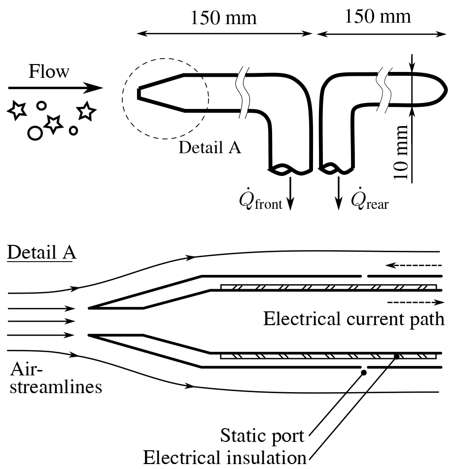
Figure 18Isokinetic probe to measure the total water content, TWC, developed at Cranfield University.
The ice particles are injected into the settling chamber of the icing wind tunnel, upstream of the spraybar system. The velocity of the particle-laden jet is about 20 m s−1, which is five times higher than the local wind tunnel airspeed. Consequently, the jet mixes and expands by turbulent mixing with the ambient airflow so that the particles are spread among the flow field and mix with the droplets atomized by the spraybar system. The particle trajectories get contracted inside the wind tunnel nozzle. Due to the circular pipe exit the ice particles also cover a circular cross sectional area inside the test section. It has been tried to extend this area by using adapters at the pipe exit and by the use of several injection pipes distributed along the settling chamber. These efforts did not work out due to ice deposits inside the additional assembly; see Baumert et al. (2016). Consequently, the simplest approach of the single pipe outlet has been chosen. For studies at glaciated and mixed phase conditions, screens and honeycombs in the settling chamber of the tunnel have to be unmounted to avoid ice accretion on these elements.
4.1 General approach
The icing wind tunnel calibration has been performed with respect to the requirements specified in SAE ARP 5905. Accordingly, both an aero-thermal calibration of the airflow and a calibration of the icing cloud had to be performed. After presenting the deployed measurement techniques, selected calibration results are presented. Finally, an instrumentation inter-comparison exercise was carried out.
4.2 PDI probe
The measurement principle of Phase Doppler interferometry (PDI) is based on light scattering interferometry (Rudoff et al., 1990) that uses as measurement scale the wavelength of light and as such its calibration is not as easily degraded. The scattering by spheres much larger than the instrument wavelength is approximated by geometrical optics. Size and velocity are determined by measuring sinusoidal scattering signals on adjacent photo-detectors as particles move through an interference fringe pattern formed in the intersection of two laser beams of same wavelength.
The method does not require frequent calibration as the light wavelength does not change and the detector separations that affect the size measurement are fixed. The sinusoidal nature of the signals detected may be used with the Fourier analysis approach to detect signals reliably even in low signal-to-noise (SNR) environments. Off-axis light scatter detection is used. The advantage of this approach is that a very small, well-defined sample volume can be formed which minimizes uncertainty when computing absolute concentration and reduces the possibility of coincident events (more than one particle residing in the sample volume at one time). The sample volume can be adjusted to balance count rate with coincidence rate to suit the user's preference. The PDI only needs an initial factory calibration since parameters affecting the measurements as the laser wavelength, beam intersection angle, transmitter and receiver focal lengths, and the detector separation do not change with age or use of the instrument.
The method has been demonstrated to be capable of measuring drop size distributions, droplet velocity distributions, size–velocity correlation, droplet time of arrival, droplet spacing, droplet number density, liquid volume flux and liquid water content. At the Braunschweig Icing Wind Tunnel, the PDI has been used for size and concentration measurements of cold clouds and for liquid or ice discrimination in mixed phase conditions. Although the PDI method cannot provide a size measurement for ice particles, it is able to extract a velocity information due to the particle's reflectivity. The resulting velocity histogram was used in an instrumentation inter-comparison campaign (see Sect. 4.6.4) in order to check differences between the mean velocity of ice particles and airspeed upstream of the 2D-S probe volume.
4.3 Cranfield isokinetic probe (IKP)
The probe consists of two tubes with one pipe faced towards the upstream direction, thereby collecting a representative sample of air, droplets and ice particles suspended within the flow; see Fig. 18. The goal is to measure the total water content (TWC) of the flow. The volume flux has to be adjusted to obtain isokineticity at the probe head. The second tube is faced downstream with its pipe end. Thus, a second sample of air, without any particles or droplets in it, can be collected to determine the water vapour content so that the quantity of water in condensed form (solid and liquid) can be determined.
A high electric current is passing through the metallic structure of the probe head thus enabling its resistive heating. Consequently, the probe stays free of an ice build-up so that the flow conditions at the entrance to the probe can be carefully matched to oncoming flow in order to achieve the correct sampling, not too rich or depleted with respect to the condensed water. The heating of the inside of the probe drives all sampled water droplets and ice particles into the vapour phase. A subsequent cooling system composed of copper tubes plunged into a water tank has been added in order to bring the air at a reasonable temperature (about 30–35 ∘C) before entering the measurement system.
The measurement system itself is mainly comprised of two parts. The first part is the mass flow meter measurement and valve to automatically control the mass flow at the probe inlet to maintain iso-kinetic conditions. The second part is the water vapour concentration measurement which is done using a LICOR 7000 system.
The probe features a double wall construction making it possible to use it as a pitot static probe and also providing a means to heat it. A large current is passed through the outer wall, via the tip and back along the inner tube. Tube wall thicknesses are chosen to get the appropriate split of heat between the different parts of the probe.
4.4 HSI probe
The high speed imaging (HSI) probe (Baumert et al., 2016) illuminates the volume using six laser beams and takes shadow images of traversing cloud particles. Thereby, depth of field errors and sampling bias due to particle obscuration are minimized. The shadow images are sampled at a frequency of 300 fps by a CMOS-chip of 640 by 480 pixels. Images of particles in the range of 5 to 1200 µm can be recorded, the resolution is 3.795 µm pixel−1. The entire device including lasers and camera is remotely controlled. A trigger beam on a different wavelength is coaxially aligned to the laser beams. A receiver, including an aperture of appropriate size and shape, is elevated to 40∘ to the transmitted beam and detects particles passing the object plane. It will trigger the lasers (laser pulse duration 12 ns) when particles are within the desired measurement volume. The HSI hardware is integrated in a cylindrical canister. Three arms, including optical components, are mounted on the front end of the canister that allow for the taking of intrusive particle images. The image processing software is able to detect and to evaluate irregular shaped particles, and includes several particle validation criteria, e.g. out-of-focus detection.
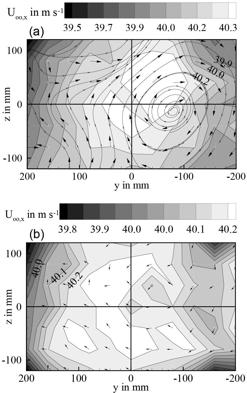
Figure 19Spatial distribution of axial flow velocity U∞,x, (a) ice-crystal-icing setup and (b) standard setup of the icing wind tunnel.
4.5 2D-S probe
The two-dimensional stereo (2D-S) probe (Lawson et al., 2006, Lawson and Baker (2006)) detects the size and concentration of cloud droplets and ice particles in the size range of 10 to 1280 µm using shadow images of the cloud particles. Two orthogonal diode laser beams illuminate two linear diode arrays consisting of 128 photodiodes with 10 µm pixel−1 resolution. When a particle crosses the laser beam in the sampling volume, its shadow image on the photodiode array is recorded by high-speed electronics. The 2D-S probe used during the airborne and wind tunnel measurements was equipped with anti-shattering tips to reduce shattering of large particles on the leading edge of the probe arms. The diode lasers operate at 45 W and are single-mode and temperature-stabilized. This design with two lasers better defines the sampling volume boundaries and thus minimizes errors associated with the depths of field and the sizing of small particles.
The LaMP 2D-S data processing has been described in detail in Leroy et al. (2016b), as it has previously been used for the treatment of the data sets collected during the HAIC field campaigns. The software is able to extract various size parameters from the particle images (area equivalent diameter, maximum dimension, etc.) and treats all major artefacts related to optical array probe's measurements, e.g. shattering, splashing, multiple particles in a single image, out of focus images. An area equivalent diameter was used in the present manuscript. For truncated images, the computation of the particle's size is based on the work of Korolev and Sussman (2000): all valid images are considered for the retrieval of the particle size distribution. The size of out-of-focus particles is corrected according to the work of Korolev (2007). The only difference between the analysis of the field campaign and the wind tunnel datasets lies in the shattering treatment as this artefact removal feature has been turned off for the wind tunnel measurements. While most shattering should be minimized by the anti-shattering tips, the shattering treatment in regions of large effective diameters and high IWC further corrects for shattering artefacts (Korolev et al., 2013). Shattering of large particles is a function of IWC; see Field et al. (2006). Since hardly any particles were larger than the full array width (see the results in Sect. 4.6.4) we argue that large particles that would have caused shattering artefacts are not present in the icing wind tunnel. Therefore, the shattering treatment was turned off.
4.6 Calibration results
4.6.1 Aerothermal calibration
An aerothermal calibration has been conducted to ensure and prove adequate airflow quality inside the test section. Investigations on airflow uniformity have been made by means of a five hole probe. The probe has been calibrated a priori based on the procedure described by Treaster and Yocum (1978). The measurements have been performed for the standard setup of the icing wind tunnel with screens and honeycombs installed in the settling chamber and also for the ice-crystal-icing setup, where these elements have been unmounted.
Figure 19a shows the contour of axial velocity inside the test section for the ice-crystal-icing setup. The pneumatic system for ice-particle conveyance was activated, the exit velocity of the conveyance pipe inside the settling chamber was about 20 m s−1, however, no ice particles were fed into the system. The plot covers a cross-sectional area of 240 mm × 400 mm around the centre-line position. Measurements have been taken in vertical and horizontal steps of 40 mm. One can clearly observe a footprint of the pneumatic-conveyance jet inside the flow field. Velocity deviations relative to the centre-line velocity are about 0.4 m s−1, which complies with ARP 5905 requirements of ±1 % spatial flow uniformity. Moreover, vectors of orthogonal velocity components are plotted, indicating a vortex inside the flow field. Since no screens and no honeycombs are installed, the vortex most likely originates from the turbulent flow interaction between conveyance piping, jet flow and surrounding tunnel air flow. The vortex magnitude is very low, local flow angularities comply with ARP 5905 specifications. For the standard setup of the icing wind tunnel, no vortex can be observed and the flow field is very uniform as shown in Fig. 19b.
Turbulence intensity has been measured by means of hot-wire anemometry. The upper part of Fig. 20 shows the contour plot of turbulence intensity for the ice-crystal-icing setup. The peak value of 1.4 % complies with ARP specifications. Again, the footprint of the pneumatic-conveyance jet is clearly visible.
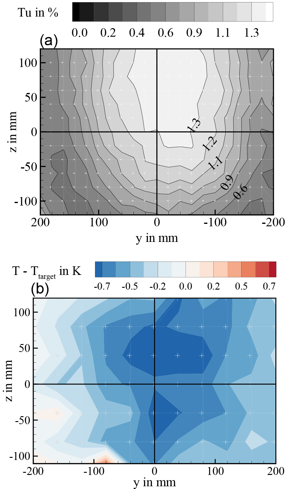
Figure 20Spatial distribution of turbulence intensity (a) and temperature variation (b) for the mixed phase configuration.
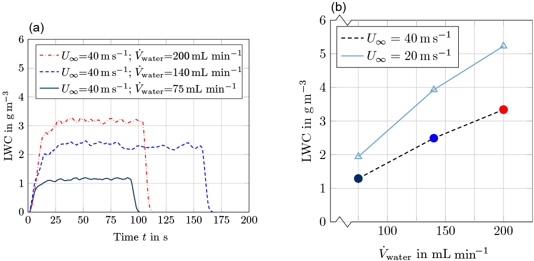
Figure 21Liquid water content calibration at the tunnel centreline based on IKP measurements, (a) LWC history and (b) LWC depending on supplied water flow rate .
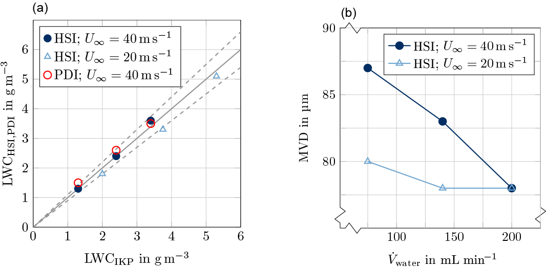
Figure 22Comparison of HSI, PDI and IKP measurements for supercooled droplet conditions: (a) optical array probes vs. IKP and (b) MVD vs. volumetric flow rate of liquid water at the spray system.
Besides flow velocity characterization, measurements of total temperature have been carried out. A very uniform temperature distribution could be verified for the standard setup of the icing wind tunnel with flow straightener and screens installed. Local temperature deviations during the measurements correspond to temporal variation of tunnel temperature, which can be adjusted with an accuracy of ±0.5 ∘C around the target value. For the ice-crystal-icing setup, a footprint of the jet can be found in the temperature field, see the lower part of Fig. 20. For a static air temperature in the wind tunnel of 0 ∘C, the local temperature at centre-line position is about −0.8 ∘C. At lower temperatures, the discrepancy diminishes since the jet temperature and the airflow temperature converge. In case of rather low temperatures of −15 ∘C, the centre-line temperature is about 0.4 K higher than the ambient temperature.
4.6.2 Calibration of the droplet cloud
Currently, two spray systems can be mounted inside the icing wind tunnel; see Sect. 2.5. The spray system with high LWC and high MVD has been calibrated by means of the Cranfield isokinetic probe (IKP), the canister PDI probe, and the modular HSI probe. IKP measurements have been conducted to correlate the liquid water content (LWC) in the centreline of the test section with the water flow rate that is supplied to the spray atomizers. The left image of Fig. 21 shows temporal plots of LWC obtained for various water flow rates at U∞ = 40 m s−1. As illustrated in the right image of Fig. 21, the dependency between LWC and flow rate is rather linear. Test points corresponding to the plots in the left image are highlighted by the same colour. For lower flow velocities U∞, higher LWCs values are obtained as anticipated in Eq. (1). Nevertheless, the LWC increase is not proportional to 1∕U∞, because the cross-sectional area of the icing cloud expands at lower wind-tunnel speeds.
Comparisons of liquid water contents derived from canister-HSI and canister-PDI measurements are plotted in the left image of Fig. 22. The dashed lines stress deviations of ±10 %. The liquid water contents assigned to C-HSI and C-PDI have been derived based on volume to mass correlations of detected droplets. It can be observed that there is very good agreement between the measurements of all three probes except for two test points of the PDI at U∞ = 20 m s−1. These measurements had been affected by water condensation inside the C-PDI. The MVD varies in the range of 80 to 95 µm, see the right image of Fig. 22. Higher MVDs have been observed with the C-PDI probe at U∞ = 40 m s−1. Presumably, droplet coalescence is promoted for higher air velocities. Yet the medium droplet size is rather constant for various liquid water contents at the same wind tunnel speed. All these results refer to the ice-crystal-icing setup with the jet switched on. No measurements have been taken away from centre-line position as neither the canister probes nor the IKP could be traversed adequately. Ice accretion studies of selected test models have proved a very uniform droplet cloud.
4.6.3 Calibration of the ice particle cloud
Ice-particle cloud calibration has been performed by means of the IKP and the canister-HSI at the centreline of the tunnel test section. Figure 23 shows time histories of the ice water content (IWC) determined by the IKP for dosing frequencies fdosing of 5 and 30 Hz at wind tunnel speeds U∞ of 20 and 40 m s−1. In the left image absolute values are plotted while the right image shows plots of IWC normalized by the target IWC. According to the IKP measurements, stable cloud conditions are established after 20 to 60 s, which is surprising, as steady state particle supply is established after 20 to 30 s. There are two possible explanations: on the one hand, there might be a slight recirculation of ice particles inside the closed-loop wind tunnel – not every injected ice particle might settle down at the forth corner of the tunnel. On the other hand, the background humidity is slowly increasing due to sublimation of the ice particle cloud, which might influence the IKP measurement. Increasing the particle supply of the dosing machine to frequencies higher than 30 Hz does not result in higher IWC, because the permeability of the sieving mesh is limited. According to Fig. 23, a maximum IWC of about 19 g m−3 can be achieved at the centre-line position. At fdosing = 5 Hz, a minimum IWC of 3 g m−3 can be adjusted. Lower feed-rates can be obtained by use of a smaller feed pipe of the dosing machine but have not been calibrated with respect to test section IWC. Figure 23 shows oscillations in IWC at low feed-rates because of an unsteady discharge of the dosing machine. This issue has been solved by the use of a rotating rod which supports particle discharge.
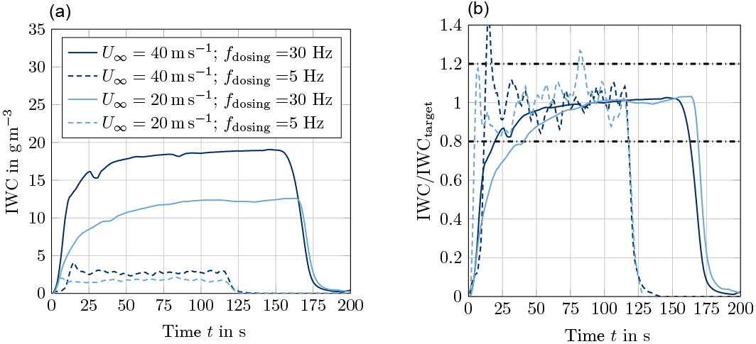
Figure 23IWC time history based on IKP measurements: (a) IWC history and (b) normalized IWC history.
Based on the IKP measurements, a linear correlation between IWC and dosing frequency has been determined. Corresponding plots are shown in the left image of Fig. 24 for wind tunnel speeds of U∞ = 20 m s−1 and U∞ = 40 m s−1. Due to the linear operational behaviour of the sieving and dosing machine, a strong linear dependence between IWC and injected ice particle mass could be demonstrated as shown in the right image of Fig. 24. This dependency allows to assess the accuracy of IWC set for a test run. For wind tunnel tests which include ice particle supply, the IWC is adjusted based on the linear fits of Fig. 24, left. The frequency of the dosing machine is set according to the demanded IWC. After a test run, the ice particle deposit on the sieving machine is weighed. Based on the correlation of dosing frequency and supplied massflow (see Fig. 17a) the ice particle massflow can be determined respecting ice deposit on the sieve. Figure 24 then allows to deduce the real IWC which has been established inside the test section. Additional test campaigns where this procedure has been applied, showed an accuracy of IWC adjustments of about ±15 %.
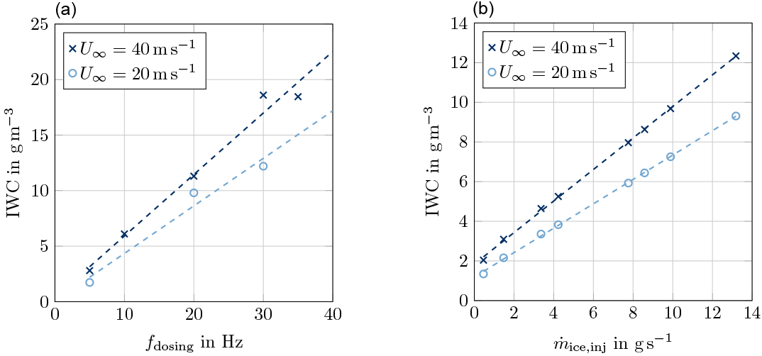
Figure 24Ice water content depending on dosing frequency fdosing and injected ice particle flow .
Investigations on spatial IWC uniformity have been performed by means of a custom-made particle-collecting tube system. The system allows to measure a relative distribution of the ice particle concentration inside the test section. A contour plot for U∞ = 40 m s−1 is shown in Fig. 25. Acceptable uniformity of ±20 % according to ARP 5905 is given for a circular area of about 150 mm in diameter. This area has proved to be sufficient and appropriate for valid icing experiments. In agreement with the turbulent footprint of the pneumatic conveyance jet, see Fig. 20, the peak IWC is located slightly above the centre-line position, which has to be respected for the mounting of aerodynamic test models.
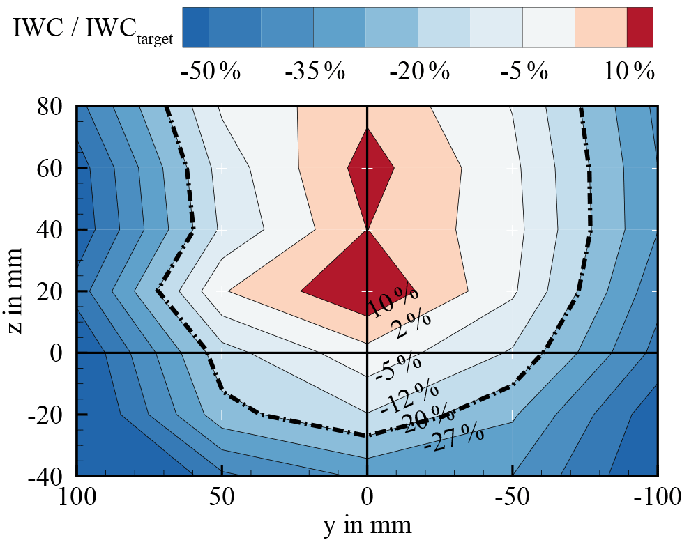
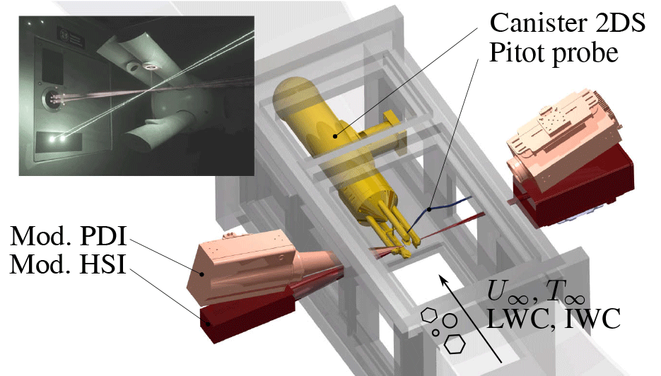
Figure 26Setup of the probe inter-comparison exercise. Alternatively to the canister 2D-S probe, which is shown here, the canister HSI probe was mounted. Upper left: C-HSI probe mounted inside the icing wind tunnel, modular PDI and HSI laser beams are adjusted close to the C-HSI sampling volume.

Figure 27Results of the probe intercomparison between 2D-S (LAMP), 2D-S (DLR), M-HSI and C-HSI for seven different test points at glaciated icing conditions.
4.6.4 Probe inter-comparison
Based on the IKP calibration, a cross comparison of various optical array probes has been performed in the Braunschweig Icing Wind Tunnel. The CNRS and DLR 2D-S probes, as well as the C-HSI have been mounted consecutively at the same position inside the test section. Additionally, modular HSI and PDI probes have been installed externally, to assess the repeatability of the test conditions. Figure 26 gives an overview of the test setup. M-PDI and M-HSI laser beams have been adjusted close to the sampling volume to perform non intrusive measurements in parallel.
Figure 27 presents a comparison of optical array probe measurements at seven glaciated cloud conditions named I01, I02, I03, I05, I06, I09 and I10. Ice water content has been derived based on the mass–size relation described by Brown and Francis (1995). Up to a diameter of 97 µm, the particles have been treated as spherical for the determination of the IWC. Above that threshold, the assumption of spherical particles would lead to an overestimation of the IWC. Ice water contents derived from measurements of both 2D-S probes and the C-HSI probe have been related to the estimated wind tunnel IWC. A rather good agreement between the measurements was proven as most of the measured values agreed with the wind tunnel prescribed IWCs with an accuracy of ±20 %, which is well within the limits of expected instrument accuracy.
Wind tunnel testing of the 2D-S probes and the C-HSI have generated a great variety of ice particle images. The upper part of Fig. 28 shows examples of ice particles captured by the C-HSI. The aggregate structure which has been observed for ice particles before fluidization and conveyance, see Fig. 13, could be maintained. The lower part of Fig. 28 shows a series of ice particle images obtained from 2D-S measurements inside the Braunschweig Icing Wind Tunnel. Note that the ice particle images were oriented vertically in a post-processing step. It can be observed that most of the particles feature an irregular, elongated shape. Based on the analyses of ice particle images one can conclude that the particles partially break up on their trajectory from the sieving machine to the tunnel test section and are reduced to smaller sizes.

Figure 28Ice particle images captured at the test section of the Braunschweig Icing Wind Tunnel. (a) images taken by C-HSI probe. (b) images taken by 2D-S probe, MMD = 79 µm, IWC = 3.2 g m−3 and T∞ = −15 ∘C.
A characteristic size distribution of artificial ice particles inside the icing wind tunnel is shown in Fig. 29a. Furthermore, particle size distributions of atmospheric ice particles (Atm) are included according to Fig. 14. The artificial ice particle cloud includes higher concentrations of small ice particles with equivalent diameters below 200 µm. The amount of particles smaller than 200 µm yielded from the wind tunnel measurements has not been identified during the airborne measurements, even for the coldest temperatures. The high amount of small ice particles is reflected in the cumulative mass distribution shown in Fig. 29b. An MMD of about 79 µm was determined for the wind tunnel icing cloud. This value agrees with the initial target of an MMD in the range of 50 to 200 µm. The HAIC flight campaigns have shown that against previous assumptions natural ice crystal clouds are characterized by higher MMDs in the range of 300 to 800 µm depending on temperature, see Fig. 29b. Yet the high number of small ice particles with MMDs below 80 µm may be of relevance for particle size distributions in young and aged contrails (Voigt et al., 2010, 2011).
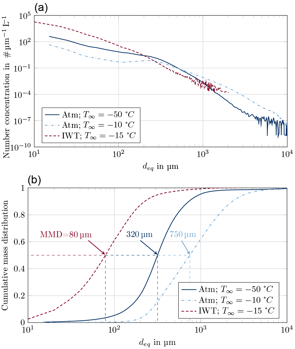
Figure 29Comparison of artificial ice particle cloud to atmospheric cloud conditions: (a) particle size distribution and (b) cumulative particle size distribution.

Figure 30Experimentally observed SLD ice shapes on a NACA0012 leading edge in the parameter space of f0 and Ac, , MVD = 80 µm and AoA . Results reproduced from Steiner and Bansmer (2016).

Figure 31Side view of ice accretion shapes on a cylinder for TWC = 12 g m−3, mr=0.12 and U∞=40 m s−1 with a variation of temperature.
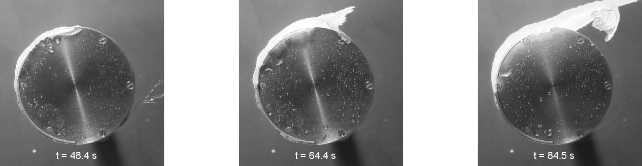
Figure 32Side view of ice accretion when heating the cylinder, ∘C, TWC = 6.8 g m−3 and mr=0.5.
It can be summarized that the initial design targets of the ice-crystal generation system have been achieved. Irregular ice particles with close agreement to natural ice particles can be injected into the wind tunnel. Even hexagonal ice crystals can be grown by cloud chamber technology and might be used for single particle impact studies. The ice particle size distribution is characterized by an MMD of about 80 µm which is between atmospheric and inside-engine particle sizes. Because the ice-crystal generation process is fully separated from icing wind tunnel operation, the MMD does not change with operating conditions. IWC values of 3 to 20 g m−3 correspond to total water contents expected for inside-engine conditions and air data probes. Lower ice water content can be adjusted by modifications of the dosing machine but require further wind tunnel calibration measurements.
5.1 Supercooled large droplets icing
The consideration of supercooled large droplets (SLD) icing is part of the certification for large transport aircraft (Politovich, 1989). Appendix O of the document EASA CS25 (EASA, 2016) provides detailed information on the MVD and LWC envelope. Outstanding requirement is the simulation of liquid clouds with median volume diameters larger than 50 µm. The trajectories of such large droplets show a large deviation from the air streamlines. With their increased inertia, the droplets might be impacting or running back in regions on the aircraft wing, which are not protected with de- or anti-icing systems.
Such SLD ice shapes and their surface roughness were investigated in the Braunschweig Icing Wind Tunnel (Steiner and Bansmer, 2016). In order to determine which wind tunnel conditions to use, they had to be related to the relevant dimensionless parameters influencing ice roughness. These are the dimensionless accumulation parameter Ac, given in Bond and Anderson (2004) as the following:
and the stagnation freezing fraction:
where ϱice represents the density of ice, δ the diameter of the inscribed circle of the airfoil nose as a reference length, free-stream pressure p and static free-stream air temperature T∞.
Within this two-dimensional (Ac and f0) parameter space, a Latin hypercube sampling was performed to define a set of experiments. The resulting ice shapes have been captured with a mould-and-cast method (Reehorst and Richter, 1987) and are shown in Fig. 30. These can be categorized into two groups: for shapes in the first group, which are marked in blue, the ice thickness was almost constant over some distance from the stagnation point and then a ridgeline appeared. Shapes in the second group were marked in red and exhibited an intense yet smooth ice accretion at the stagnation line followed by a much rougher zone with a feather structure.
5.2 Mixed phase icing of a cylinder
Comprehensive investigations on ice accretion of generic test models at mixed phase conditions have been performed in the recent past (Bansmer and Baumert, 2017; Baumert et al., 2018). The test models have been equipped with heat foils to investigate the effect of internal heat conduction on the accretion process.
Figure 31 shows ice shapes on a cylinder model without heat foil operation. A mixed phase cloud with a total water content of 12 g m−3 and a melting ratio mr (defined as LWC ∕ TWC in this setup) of 0.12 has been adjusted. The static air temperature has been varied between 0 and −15 ∘C. In contrast to supercooled droplet icing, the ice accretion for mixed-phase icing exhibits a conical shape. The ice accretion process appears to be strongly dependent on air temperature. At constant melting ratio and constant total water content, a decrease in icing severity can be observed for lower temperatures. This effect can be addressed to supercooling of the liquid droplets inside the mixed phase clouds. At lower temperatures enhanced supercooling allows a large amount of liquid to freeze with only a short delay upon impact. Therefore, less liquid is locally available to promote ice particle sticking resulting in a significantly reduced ice accretion. Water imbibition into the supposed porous ice layer seems therefore a necessary condition for increased icing severity.
Figure 32 gives an example of mixed phase icing of the cylinder with activated heat foils. In contrast to Fig. 31, no cone shaped ice accretion develops as the accretion layer constantly melts due to internal heating. Consequently, the accretion does not adhere to the cylinder surface and gets dragged towards the upper side of the cylinder by shear forces induced by the ambient airflow. Capillary forces prevent the accretion layer from instant shedding. As the accretion layer convects downstream, further ice accumulates in the flow stagnation area of the cylinder. In consequence, a cohesive ice accretion structure detaches from the cylinder and growths further downstream.
5.3 Development of measurement techniques
The experimental characterization of multiphase flows in icing wind tunnels can be very challenging and is a fruitful topic for developing measurement techniques as already shown in Sect. 4. Here, we want to shortly summarize an optical technique to measure the 3-D geometry of ice accretion.
Two properties of ice accretion are particularly demanding for optical measurement techniques. On the one hand, the ice surface geometry is very complex and includes both large roughness elements and deep chasms, see again Fig. 30. On the other hand, glaze ice formations appear transparent in the visible light range, which makes them hard to detect with conventional camera systems (Gong and Bansmer, 2015b). Therefore, we developed a general approach based on mid-infrared (MIR) laser scanning (Gong and Bansmer, 2015a), because MIR radiation penetrates ice and water only within a depth of less than 10 µm.
The MIR-line scanning method uses a CO2-laser light sheet, which is first created through proper lenses, and then projected onto the scene. The ice surface will absorb this light and emit an infrared radiation signature, which is visible as a deformed line. Using a properly calibrated camera, the deformed line can be transformed using a triangulation function yielding 3-D coordinates. While consecutively scanning with the laser light sheet over the object, the entire 3-D ice geometry can be reconstructed. The scanning accuracy was validated with 3-D ice objects of known dimensions; a pattern of frustums was used.
Operating the icing wind tunnel with prototype test models requires intervention and human surveillance. In particular, activities inside the icing wind tunnel or in the cooling chamber (see ➇ in Fig. 4) can be very exhausting and have to be considered for health and safety. According to Ramsey et al. (1983), unsafe behaviour significantly increases when the ambient wet-bulb temperature is lower than 10 ∘C, although workers are appropriately clothed. Frequent crew change is thus a necessary measure to perform these exhausting activities.
Another safety aspect is water handling with respect to Legionella. These bacteria multiply with ideal growth rates between 32 to 42 ∘C and can infect alveolar macrophages, which may result in several lung diseases. The water, which is to be sprayed inside the icing wind tunnel is increasing this threat since the contaminated droplets smaller than 10 µm can be deeply inhaled. To minimize this risk, demineralized water is used that is further sterilized with ultraviolet radiation before entering the pneumatic atomizers.
The presented data are subject to several legal agreements with the funding bodies that are mentioned in the acknowledgements. This data is thus available only on request. Please contact Stephan Bansmer for wind tunnel calibration data and Alfons Schwarzenboeck/Christiane Voigt for ice particle data that was gathered during the Darwin and Cayenne campaign.
Roman symbols
| a | speed of sound, m s−1 |
| A | area, m2 |
| Ac | accumulation parameter |
| AH | absolute humidity, g m−3 |
| c | chord length of an airfoil, m |
| cD | drag coefficient of a droplet |
| clatent | specific latent heat of fusion, kJ kg−1 |
| cp | specific heat capacity at constant pressure, |
| d | diameter of a droplet, µm |
| D | drag force vector, 1⋅N |
| f0 | stagnation line freezing fraction |
| fdosing | dosing frequency, Hz |
| g | gravitational acceleration vector, |
| IWC | ice water content, g m−3 |
| k | heat conductivity, |
| K | contraction of the wind-tunnel nozzle |
| L | length of the wind-tunnel nozzle, m |
| LWC | liquid water content, g m−3 |
| m | mass, kg |
| mass flow rate, kg s−1 | |
| mr | melting ratio |
| Ma | Mach number |
| MVD | median volume diameter, µm |
| MMD | median mass diameter, µm |
| Nu | Nusselt number |
| p | pressure, Pa |
| P | power, W |
| Pr | Prandtl number |
| heat, W | |
| R | specific gas constant, |
| Re | Reynolds number |
| RH | relative humidity |
| 𝒮spray | operational state of the spray system |
| t | time, s |
| tacc | accumulation time, s |
| T | static temperature, K |
| Tu | turbulence level |
| TWC | total water content, g m−3 |
| u, w | velocity components in x and z direction, m s−1 |
| U∞ | freestream velocity of air, m s−1 |
| volumetric flow rate, m3 s−1 | |
| x, z | Cartesian coordinates, m |
Greek symbols
| α | Angle of attack, deg |
| β, γ | fitting constants for particle sizing |
| δ | twice the nose radius of an airfoil, m |
| Δ | difference, e.g. in temperature or in velocity |
| ζ | specific loss coefficient |
| η | efficiency |
| λ | power factor |
| μ | dynamic viscosity, |
| ϱ | density, kg m−3 |
Subscripts
| air | air |
| chill | chilling |
| d | droplet |
| eq | equivalent |
| fan | fan |
| HE | heat exchanger |
| HSI | high-speed imaging probe |
| ice | ice |
| inj | injected |
| IKP | isokinetic probe |
| jet | jet |
| latent | latent |
| max | maximum |
| nozzle | wind tunnel nozzle |
| PDI | phase Doppler interferometry |
| sc | settling chamber |
| sensible | sensible |
| target | target value |
| tsec | test section |
| tot | total |
| vapour | vapour |
| water | water |
| wb | wet bulb |
| x | in x direction |
| ∞ | freestream condition |
The authors declare that they have no conflict of interest.
The presented work was conducted within the framework of the DLR@Uni
programme SuLaDI, which is founded by the Helmholtz Association. The ice-crystal-icing capability was achieved by funding from the European Union's
Seventh Framework Programme in research, technological development and
demonstration under grant agreement no. ACP2-GA-2012-314314. The improved
spray system was funded by the German Federal Ministry of Economic Affairs
and Energy, grant number Drífa-FKZ0325842A. Some of the contributed
computational results were obtained thanks to Wagdi Habashi (McGill university, Canada) and the funding of the German
Research Foundation, DFG grant BA4953/2-1. Christiane Voigt and Tina
Jurkat-Witschas have been funded by the Helmholtz Society under contract no.
W2/W3-060 and the German Science Foundation within DFG SPP 1294 HALO by grant
VO1504/4-1 and grant JU 3059/1-1. Figure 3
was supported by Daniel Hattenbach (Greencooltec GmbH) and
Figure 4 was supported by Walter Arnold
(Berlin). The authors further express their thanks to all project partners
from Europe and overseas and acknowledge the support of the German Research Foundation and the Open Access Publication Funds of the Technische Universität Braunschweig.
Edited by: Wiebke Frey
Reviewed by: Dan Fuleki and David Hammond
Al-Khalil, K., Salamon, L., and Tenison, G.: Development of the Cox icing research facility, in: 36th Aerospace Sciences Meeting & Exhibit, AIAA, Citeseer, 1998. a
Bansmer, S. E. and Baumert, A.: From high altitude clouds to an icing wind tunnel: en route to understand ice crystal icing, in: Proceedings of the EUCASS Conference held in Milano, Italy, 2017. a
Baumert, A., Bansmer, S., Sattler, S., Pervier, H., and Esposito, B.: Simulating natural ice crystal cloud conditions for icing wind tunnel experiments – A review on the design, commissioning and calibration of the TU Braunschweig ice crystal generation system, in: AIAA AVIATION Forum, American Institute of Aeronautics and Astronautics, https://doi.org/10.2514/6.2016-4053, 2016. a, b
Baumert, A., Bansmer, S., Trontin, P., and Villedieu, P.: Experimental and numerical investigations on aircraft icing at mixed phase conditions, Int. J. Heat Mass Tran., 123, 957–978, 2018. a
Beaugendre, H., Morency, F., and Habashi, W. G.: FENSAP-ICE's Three-Dimensional In-Flight Ice Accretion Module: ICE3D, J. Aircraft, 40, 239–247, https://doi.org/10.2514/2.3113, 2003. a
Bond, T. H. and Anderson, D. N.: Manual of Scaling Methods, NASA/CR-2004-212875, 2004. a, b
Braga, R. C., Rosenfeld, D., Weigel, R., Jurkat, T., Andreae, M. O., Wendisch, M., Pöhlker, M. L., Klimach, T., Pöschl, U., Pöhlker, C., Voigt, C., Mahnke, C., Borrmann, S., Albrecht, R. I., Molleker, S., Vila, D. A., Machado, L. A. T., and Artaxo, P.: Comparing parameterized versus measured microphysical properties of tropical convective cloud bases during the ACRIDICON–CHUVA campaign, Atmos. Chem. Phys., 17, 7365–7386, https://doi.org/10.5194/acp-17-7365-2017, 2017. a
Brown, P. and Francis, P.: Improved Measurements of the Ice Water Content in Cirrus Using a Total-Water Probe, J. Atmos. Ocean. Tech., 12, 410–414, 1995. a
Connolly, P. J., Emersic, C., and Field, P. R.: A laboratory investigation into the aggregation efficiency of small ice crystals, Atmos. Chem. Phys., 12, 2055–2076, https://doi.org/10.5194/acp-12-2055-2012, 2012. a
Currie, T., Struk, P., Tsao, J.-C., Fuleki, D., and Knezevici, D.: Fundamental Study of Mixed-Phase Icing with Application to Ice Crystal Accretion in Aircraft Jet Engines, in: Fluid Dynamics and Co-located Conferences, American Institute of Aeronautics and Astronautics, https://doi.org/10.2514/6.2012-3035, 2012. a, b
Currie, T. C., Fuleki, D., and Mahallati, A.: Experimental studies of mixed-phase sticking efficiency for ice crystal accretion in jet engines, in: 6th AIAA Atmospheric and Space Environments Conference, p. 3049, 2014. a
Dezitter, F., Grandin, A., Brenguier, J., Hervy, F., Schlager, H., Villedieu, P., and Zalamansky, G.: HAIC (High Altitude Ice Crystals), 5th AIAA Atmospheric and Space Environments Conference, AIAA-2013-2674, 2013. a
EASA: Certification Specifications and Acceptable Means of Compliance for Large Aeroplanes CS-25, Amendment 18, available at: https://www.easa.europa.eu/sites/default/files/dfu/CS-25 Amendment 18_0.pdf (last access: 18 May 2018), 2016. a, b
Farzaneh, M.: Atmospheric Icing of Power Networks, Springer Netherlands, Dordrecht, https://doi.org/10.1007/978-1-4020-8531-4, 2008. a
Feulner, M., Liao, S., Rose, B., and Liu, X.: Ice Crystal Ingestion in a Turbofan Engine, SAE 2015 International Conference on Icing of Aircraft, Engines and Structures, 2015. a
Field, P., Heymsfield, A., and Bansemer, A.: Shattering and particle interarrival times measured by optical array probes in ice clouds, J. Atmos. Ocean. Tech., 23, 1357–1371, 2006. a
Finstad, K. J., Lozowski, E. P., and Makkonen, L.: On the median volume diameter approximation for droplet collision efficiency, J. Atmos. Sci., 45, 4008–4012, 1988. a
Flegel, A. B. and Oliver, M. J.: Preliminary Results from a Heavily Instrumented Engine Ice Crystal Icing Test in a Ground Based Altitude Test Facility, in: 8th AIAA Atmospheric and Space Environments Conference, p. 3894, 2016. a
Fontaine, E., Schwarzenboeck, A., Delanoë, J., Wobrock, W., Leroy, D., Dupuy, R., Gourbeyre, C., and Protat, A.: Constraining mass–diameter relations from hydrometeor images and cloud radar reflectivities in tropical continental and oceanic convective anvils, Atmos. Chem. Phys., 14, 11367–11392, https://doi.org/10.5194/acp-14-11367-2014, 2014. a
Gayet, J.-F., Shcherbakov, V., Bugliaro, L., Protat, A., Delanoë, J., Pelon, J., and Garnier, A.: Microphysical properties and high ice water content in continental and oceanic mesoscale convective systems and potential implications for commercial aircraft at flight altitude, Atmos. Chem. Phys., 14, 899–912, https://doi.org/10.5194/acp-14-899-2014, 2014. a
Gent, R. W., Dart, N. P., and Cansdale, J. T.: Aircraft icing, Philos. T. R. Soc. A, 358, 2873–2911, https://doi.org/10.1098/rsta.2000.0689, 2000. a
GL: Rules and Guidelines Industrial Services – Guideline for the Certification of Wind Turbines, 2010. a
Gong, X. and Bansmer, S.: 3-D ice shape measurements using mid-infrared laser scanning, Opt. Express, 23, 4908–4926, 2015a. a
Gong, X. and Bansmer, S.: Laser scanning applied for ice shape measurements, Cold Reg. Sci. Tech., 115, 64–76, 2015b. a
Grzych, M. and Mason, J.: Weather Conditions Accociated with Jet Engine Power-loss and Damage due to Ingestion of Ice Particles: What We've Learned Through 2009, 14th Conference of Aviation, Range and Aerospace Meteorology, 2010. a
Hochart, C., Fortin, G., Perron, J., and Ilinca, A.: Wind turbine performance under icing conditions, Wind Energy, 11, 319–333, https://doi.org/10.1002/we.258, 2008. a
IPHWG: Working Group Report on Supercooled Large Droplet Rulemaking, Transport Airplane Directorate, Task, 2, 11 pp., available at: http://lessonslearned.faa.gov/AmericanEagle/IPHWG.pdf (last access: 18 May 2018), 2005. a
Jung, S., Tiwari, M. K., Doan, N. V., and Poulikakos, D.: Mechanism of supercooled droplet freezing on surfaces, Nat. Commun., 3, 615, https://doi.org/10.1038/ncomms1630, 2012. a, b
Knudsen, J. G. and Katz, D. L.: Fluid dynamics and heat transfer, McGraw-Hill Book Company, 1958. a
Korolev, A.: Reconstruction of the sizes of spherical particles from their shadow images. Part I: Theoretical considerations, J. Atmos. Ocean. Tech., 24, 376–389, 2007. a
Korolev, A. and Sussman, B.: A technique for habit classification of cloud particles, J. Atmos. Ocean. Tech., 17, 1048–1057, 2000. a
Korolev, A., Emery, E., and Creelman, K.: Modification and tests of particle probe tips to mitigate effects of ice shattering, J. Atmos. Ocean. Tech., 30, 690–708, 2013. a
Lamb, D. and Verlinde, J.: Physics and Chemistry of Clouds, Cambridge University Press, cambridge Books Online, 2011. a
Langmuir, I.: The collected works of Irving Langmuir, vol. 10 – Atmospheric phenomena, chap. Mathematical investigation of water droplet trajectories, 335–393, Pergamon press, 1961. a
Lawson, R. and Baker, B.: Improvement in determiination of ice water content from two-dimensional particle imagery. Part II: Applications to collected data, J. Appl. Meteorol. Clim., 45, 1292–1303, 2006. a
Lawson, R., O'Connor, D., Zmarzly, P., Weaver, K., Baker, B., Mo, Q., and Jonsson, H.: The 2D-S (Stereo) probe: design and preliminary tests of a new airborne, high speed, high-resolution particle imaging probe, J. Atmos. Ocean. Tech., 23, 1462–1477, 2006. a
Leroy, D., Fontaine, E., Schwarzenboeck, A., Strapp, J., Lilie, L., Delanoe, J., Protat, A., Dezitter, F., and Grandin, A.: HAIC/HIWC Field Campaign – Specific Findings on PSD Microphysics in High IWC Regions from In Situ Measurements: Median Mass Diameters, Particle Size Distribution Characteristics and Ice Crystal Shapes, SAE Technical Paper 2015-01-2087, SAE 2015 International Conference on Icing of Aircraft, Engines and Structures, 2015. a
Leroy, D., Coutris, P., Fontaine, E., Schwarzenboeck, A., Strapp, J., Lilie, L., Korolev, A., McFarqhuar, G., Dezitter, F., and Calmes, A.: HAIC/HIWC field campaigns – specific findings on ice crystal characteristics in high ice water content cloud regions, 8th AIAA Atmospheric and Space Environments Conference, 2016a. a
Leroy, D., Fonaine, E., Schwarzenboeck, A., and Strapp, J.: Ice Crystal Sizes in High Ice Water Content Clouds. Part I: On the Computation of Median Mass Diameter from In Situ Measurements. Part I: On the Computation of Median Mass Diameter from In Situ Measurements, J. Atmos. Ocean. Tech., 33, 2461–2476, 2016b. a, b, c
Leroy, D., Fontaine, E., Schwarzenboeck, A., Strapp, J., Korolev, A., McFarquhar, G., Dupuy, R., Gourbeyre, C., Lilie, L., Protat, A., Delanoue, J., Dezitter, F., and Grandin, A.: Ice Crystal Sizes in High Ice Water Content Clouds. Part II: Statistics of Mass Diameter Percentiles in Tropical Convection Observed during the HAIC/HIWC Project, J. Atmos. Ocean. Tech., 34, 117–136, 2017. a, b
Makkonen, L.: Estimation of wet snow accretion on structures, Cold Reg. Sci. Technol., 17, 83–88, https://doi.org/10.1016/S0165-232X(89)80018-7, 1989. a
Mason, J., Strapp, J., and Chow, P.: The Ice Particle Threat to Engines in Flight, 44th AIAA Aerospace Sciences Meeting and Exhibit, AIAA-2006-206, 2006. a, b
Messinger, B. L.: Equilibrium temperature of an unheated icing surface as a function of air speed, J. Aeronaut. Sci., 20, 29–42, 1953. a, b
Mulherin, N.: Atmospheric icing and communication tower failure in the United States, Cold Reg. Sci. Technol., 27, 91–104, https://doi.org/10.1016/S0165-232X(97)00025-6, 1998. a
Oleskiw, M. M., Hyde, F. H., and Penna, P. J.: In-Flight Icing Simulation Capabilities of NRC's Altitude Icing Wind Tunnel, in: 39th AIAA Aerospace Sciences Meeting & Exhibit, AIAA-2001-0094, https://doi.org/10.2514/6.2001-94, 2001. a
Oliver, M.: Validation Ice Crystal Icing Engine Test in the Propulsion System Laboratory at NASA Glenn Research Center, 6th AIAA Atmospheric and Space Environments Conference, AIAA-2014-2898, 2014. a
Pastor-Barsi, C., Arrington, A., and VanZante, J. F.: Aero-Thermal Calibration of the NASA Glenn Icing Research Tunnel (2012 Test), NASA Technical Report E-18454-1, 2012. a
Politovich, M. K.: Aircraft Icing Caused by Large Supercooled Droplets, J. Appl. Meteorol., 28, 856–868, https://doi.org/10.1175/1520-0450(1989)028<0856:AICBLS>2.0.CO;2, 1989. a, b
Ramsey, J. D., Burford, C. L., Beshir, M. Y., and Jensen, R. C.: Effects of workplace thermal conditions on safe work behavior, J. Safety Res., 14, 105–114, 1983. a
Reehorst, A. L. and Richter, G. P.: New Methods and Materials for Molding and Casting Ice Formations, Tech. Rep. NASA-TM-100126, NASA Lewis Research Center, 1987. a
Rudoff, R., Smith, J., and Bachalo, W.: Development of a Phase Doppler Based Probe for Icing Cloud Droplet Characterization, 28th Aerospace Sciences Meeting, Reno Nevada, 1990. a
Scheiman, J. and Brooks, J.: Comparison of Experimental and Theoretical Turbulence Reduction from Screens, Honeycomb, and Honeycomb-Screen Combinations, J. Aircraft, 18, 638–643, 1981. a
Schremb, M. and Tropea, C.: Solidification of supercooled water in the vicinity of a solid wall, Phys. Rev. E, 94, 052804, https://doi.org/10.1103/PhysRevE.94.052804, 2016. a
Simpson, R. L.: Junction flows, Annu. Rev. Fluid Mech., 33, 415–443, 2001. a
Steiner, J. and Bansmer, S.: Ice Roughness and its Impact on the Ice Accretion Process, in: 8th AIAA Atmospheric and Space Environments Conference, p. 3591, 2016. a, b
Strapp, J., Korolev, A., Ratvasky, T., Potts, R., Protat, A., May, P., Ackerman, A., Fridlind, A., Minnis, P., Haggerty, J., Riley, J., Lilie, L., and Isaac, G.: The High Ice Water Content Study of Deep Convective Clouds: Report on Science and Technical Plan, techreport, Federal Aviation Administration, FAA Rep. DOT/FAA/TC-14/31, 105 pp., available at: http://www.tc.faa.gov/its/worldpac/techrpt/tc14-31.pdf (last access: 18 May 2018), 2016. a
Treaster, A. L. and Yocum, A. M.: The calibration and application of five-hole probes, Tech. Rep. TM 78-10, Pennsylvania State University, institute for science and engineering, applied research laboratory, 1978. a
Uberoi, M. S.: Effect of Wind-Tunnel Contraction on Free-Stream Turbulence, J. Aeronaut. Sci., 23, 754–764, 1956. a
Vecchione, L. and De Matteis, P.: An overview of the CIRA icing wind tunnel, in: 41st Aerospace Sciences Meeting and Exhibit, p. 900, 2003. a
Voigt, C., Schumann, U., Jurkat, T., Schäuble, D., Schlager, H., Petzold, A., Gayet, J.-F., Krämer, M., Schneider, J., Borrmann, S., Schmale, J., Jessberger, P., Hamburger, T., Lichtenstern, M., Scheibe, M., Gourbeyre, C., Meyer, J., Kübbeler, M., Frey, W., Kalesse, H., Butler, T., Lawrence, M. G., Holzäpfel, F., Arnold, F., Wendisch, M., Döpelheuer, A., Gottschaldt, K., Baumann, R., Zöger, M., Sölch, I., Rautenhaus, M., and Dörnbrack, A.: In-situ observations of young contrails – overview and selected results from the CONCERT campaign, Atmos. Chem. Phys., 10, 9039–9056, https://doi.org/10.5194/acp-10-9039-2010, 2010. a
Voigt, C., Schumann, U., Jessberger, P., Jurkat, T., Petzold, A., Gayet, J.-F., Krämer, M., Thornberry, T., and Fahey, D.: Extinction and optical depth of contrails, Geophys. Res. Lett., 38, https://doi.org/10.1029/2011GL047189, 2011. a
Voigt, C., Schumann, U., Minikin, A., Abdelmonem, A., Afchine, A., Borrmann, S., Boettcher, M., Buchholz, B., Bugliaro, L., Costa, A., et al.: ML-CIRRUS: The Airborne Experiment on Natural Cirrus and Contrail Cirrus with the High-Altitude Long-Range Research Aircraft HALO, B. Am. Meteorol. Soc., 98, 271–288, https://doi.org/10.1175/BAMS-D-15-00213.1, 2017. a
Wagner, B.: Ice Accretion Simulation, Tech. Rep. AGARD report no. 344, North Atlantic Treaty Organization, 1997. a
Wendisch, M., Pöschl, U., Andreae, M. O., Machado, L. A., Albrecht, R., Schlager, H., Rosenfeld, D., Martin, S. T., Abdelmonem, A., Afchine, A., et al.: ACRIDICON–CHUVA Campaign: Studying Tropical Deep Convective Clouds and Precipitation over Amazonia Using the New German Research Aircraft HALO, B. Am. Meteorol. Soc., 97, 1885–1908, https://doi.org/10.1175/BAMS-D-14-00255.1, 2016. a
Yao, S.-C. and Schrock, V.: Heat and mass transfer from freely falling drops, J. Heat Transf., 98, 120–126, 1976. a
Zerr, R. J.: Freezing Rain: An Observational and Theoretical Study, J. Appl. Meteorol., 36, 1647–1661, https://doi.org/10.1175/1520-0450(1997)036<1647:FRAOAT>2.0.CO;2, 1997. a
- Abstract
- Introduction
- Design and construction of the Braunschweig Icing Wind Tunnel
- Ice crystals and mixed phase capability
- Commissioning of the Braunschweig Icing Tunnel
- Some applications and test results
- Health and safety
- Data availability
- Appendix A: Nomenclature
- Competing interests
- Acknowledgements
- References